Pion transition form factor and distribution amplitudes in large-$N_{c}$ Regge models

Abstract

We analyze the $\pi\gamma^{\ast}\gamma^{\ast}$ amplitude in the framework of radial Regge models in the large-$N_{c}$ limit. With the assumption of similarity of the asymptotic Regge $\rho$ and $\omega$ meson spectra we find that the pion distribution amplitude is constant in the large-$N_{c}$ limit at the scale $Q_{0}$ where the QCD radiative corrections are absent – a result found earlier in a class of chiral quark models. We discuss the constraints on the couplings from the anomaly and from the limit of large photon virtualities, and find that the coupling of the pion to excited $\rho$ and $\omega$ mesons must be asymptotically constant. We also discuss the effects of the QCD evolution on the pion electromagnetic transition form factor. Finally, we use the Regge model to evaluate the slope of the form factor at zero momentum and compare the value to the experiment, finding very reasonable agreement.

I Introduction

The study of exclusive processes in QCD Lepage and Brodsky (1980); Chernyak and Zhitnitsky (1984) has been a permanent challenge both on the theoretical as well as the experimental side. The production of neutral pions by two virtual photons provides the simplest process where both perturbative and non-perturbative aspects of strong interactions can be tested. Indeed, the normalization of the corresponding from factor for real photons is dictated by the chiral anomaly. In the opposite limit of large photon virtualities the amplitude factorizes into power corrections and a soft and scale dependent distribution amplitude (DA) which gives direct information on the quark content of the pion at a given scale. Actually, for large momenta the behavior of the DA is controlled by the perturbative QCD renormalization group evolution Lepage and Brodsky (1980); Dittes and Radyushkin (1981); Mueller (1995) in terms of Gegenbauer polynomials as implied by the conformal symmetry (for a review see, e.g., Ref. Braun et al. (2003)) and the high-$Q^{2}$ power expansion. Then at $Q^{2}\to\infty$ one has the fixed point result, e.g., $\varphi^{(2)}(x,Q^{2})\to 6x(1-x)$. For low scales genuinely non-perturbative evolution can be tackled by transverse lattice methods Dalley (2001); Burkardt and Seal (2002) (for a review see e.g. Ref. Burkardt and Dalley (2002)). The first and second moments of the DA have been computed on Euclidean lattices Del Debbio et al. (2003); Del Debbio (2005); Gockeler et al. (2005). The QCD sum rules have been applied to the leading twist-2 DA Belyaev and Johnson (1997). Measurements of the transition form factor have been undertaken by the CELLO Behrend et al. (1991) and CLEO Gronberg et al. (1998) collaborations. An analysis of the lowest Gegenbauer moments $a_{2}$ and $a_{4}$ has been carried out by Schmedding and Yakovlev (2000) and Bakulev et al. (2001, 2003); Bakulev et al. (2004a); Bakulev et al. (2006). Higher twists have been analyzed in the context of light cone sum rules Agaev (2005). A direct measurement of the DA has been presented by the E791 collaboration Aitala et al. (2001). For a concise review on all these developments see, e.g., Ref. Bakulev et al. (2004b) and references therein.

Most calculations dealing with the pion transition form factor and more specifically with the DA involve quarks as explicit degrees of freedom. This appears rather natural but the principle of the quark-hadron duality suggests that it should also be possible to make these calculations entirely in terms of the complete set of hadronic states. In fact, the large $N_{c}$-limit of QCD ’t Hooft (1974); Witten (1979) makes quark-hadron duality manifest at the expense of introducing an infinite number of weakly interacting stable mesons and glueballs. The large-$N_{c}$-limit may in fact be regarded as a model-independent formulation of the quark model. Actually, chiral quark models are particular realizations implementing in a rather natural way this large-$N_{c}$ behavior at the one-quark-loop approximation and several calculations have been made along these lines Petrov and Pobylitsa (1997); Petrov et al. (1999); Heinzl (2001); Praszalowicz and Rostworowski (2001); Anikin et al. (2001, 2000a); Dorokhov et al. (2003); Dorokhov (2003); Ruiz Arriola and Broniowski (2002, 2003) (for a review see, e.g., Ref. Ruiz Arriola (2002)). Despite the subtleties regarding the correct implementation of chiral Ward identities Ruiz Arriola (2002); Bzdak and Praszalowicz (2003), chiral quark models by themselves cannot be “better” than the large-$N_{c}$ limit, as they form a particular model realization of this limit. Surprisingly, up to now there has been remarkable little information on the quark content of hadrons based solely and directly on the large-$N_{c}$ limit and the quark-hadron duality ideas, without resorting to specific low-energy quark models.

The purpose of this paper is to fill this gap and analyze the pion transition form factor in the original spirit of the large-$N_{c}$ limit. We impose chiral constraints at low energies and QCD short distance constraints at high energies and extract from there the DA in a Regge model with infinitely many resonances where the radial squared mass spectrum is assumed to be linear. This near-linearity is supported by the experimental analysis of Ref.  Anisovich et al. (2000). We do the analysis in the absence of radiative corrections which must be introduced via QCD evolution, hence our calculation corresponds to some reference scale $Q_{0}$ where the radiative QCD corrections are absent. Remarkably, we obtain the same main result as found previously by us in chiral quark models Ruiz Arriola and Broniowski (2002, 2003), namely, the leading-twist pion DA is constant at the scale $Q_{0}$. Our calculation provides an explicit example of quark-hadron duality in an exclusive process.

Up till now the calculations within the framework of large-$N_{c}$ Regge models have been mainly restricted to two-point functions Golterman and Peris (2001); Simonov (2002); Golterman and Peris (2003); Afonin et al. (2004); Afonin and Espriu (2006); Ruiz Arriola and Broniowski (2006). On the other hand, large-$N_{c}$-motivated calculations of three-point functions with short distance constraints have been carried out with a finite number of resonances, which enabled getting model-independent results for vector meson decays Moussallam (1995); Knecht and Nyffeler (2001); Beane (2001a, b); Ruiz-Femenia et al. (2003). In this regard there are large $N_{c}$ studies of both the pion Dominguez (2001) and the proton Dominguez and Thapedi (2004) electromagnetic form factors. It should also be mentioned that, echoing some older ideas of Radyushkin Radyushkin (1995), the light-cone wave functions have recently been computed within the holographic approach to QCD based on the AdS/CFT correspondence Brodsky and de Teramond (2006b, a) or meromorphization ideas  Radyushkin (2006). In these works the quark-hadron duality is also exploited.

The outline of the paper is as follows. In Sect. II we review DAs in the large-$N_{c}$ context and fix our notation for the remainder of the paper. In Sect. III we undertake the analysis of the large-$N_{c}$ Regge model and its consequences for the pion transition form factor and pion DA. Section IV deals with aspects of the QCD evolution, which is a crucial ingredient of analyses of this kind. For completeness some technical details of the LO evolution of the non-singlet DA are provided in Appendix A.

II parton Distribution Amplitude and large $N_{c}$

Partonic distribution amplitudes (DAs) are basic properties of bound states of QCD. They are defined as matrix elements of quark bilinears between the vacuum and the hadronic state in question. For instance, the twist-2 DA of $\pi^{a}$, $\varphi^{(2)}(x)$, is given by

$$\langle 0|\overline{\psi}(z)\gamma_{\mu}\gamma_{5}\frac{\tau^{a}}{2}[z,-z]\psi(-z)|\pi^{a}(q)\rangle$$ (1)

$$= if_{\pi}(q^{2})q_{\mu}\int_{0}^{1}dxe^{iuq\cdot z}\varphi^{(2)}(x),$$

where $u=2x-1$, $z$ is a coordinate along the light cone, $[z,-z]$ denotes the gauge link operator, and $f_{\pi}(q^{2})$ is the pion decay form factor, with the pion decay constant $f_{\pi}(0)\equiv f=86$ MeV in the chiral limit. The DAs have the support $x\in[0,1]$, normalization $\int_{0}^{1}dx\,\varphi(x)=1$, and satisfy the crossing relation $\varphi(x)=\varphi(1-x)$. Obviously the definition (1) requires an identification of quark degrees of freedom and also specification of a renormalization scale and scheme.

On the other hand, the pion DA is related to the pion electromagnetic transition form factor in the process $\gamma^{\ast}\gamma^{\ast}\to\pi^{0}$, or more generally, to processes with one pion and two (virtual or real) photons on external legs. This is a physical matrix element which does not depend on the renormalization scale and which is more suitable for our purposes. With the outgoing momenta and polarizations of the photons denoted as $q_{1}$,$e_{1}$ and $q_{2}$, $e_{2}$ one finds the amplitude

$$\Gamma^{\mu\nu}_{\pi^{0}\gamma^{\ast}\gamma^{\ast}}(q_{1},q_{2}) = \epsilon_{\mu\nu\alpha\beta}e_{1}^{\mu}e_{2}^{\nu}q_{1}^{\alpha}q_{2}^{\beta}F_{\pi\gamma^{\ast}\gamma^{\ast}}(Q^{2},A),$$ (2)

where the pion transition form factor $F_{\pi\gamma^{\ast}\gamma^{\ast}}$ depends on the total virtuality, $Q^{2}$, and the photon asymmetry, $A$,

$$Q^{2}=-(q_{1}^{2}+q_{2}^{2}),\;A=\frac{q_{1}^{2}-q_{2}^{2}}{q_{1}^{2}+q_{2}^{2}},\;-1\leq A\leq 1.$$ (3)

Equivalently, $q_{1}^{2}=-\frac{(1+A)}{2}Q^{2}$, $q_{2}^{2}=-\frac{(1-A)}{2}Q^{2}$. For large virtualities one finds the standard twist decomposition of the pion transition form factor Lepage and Brodsky (1980),

$$F_{\pi^{0}\gamma^{\ast}\gamma^{\ast}}(Q^{2},A)=J^{(2)}(A)\frac{1}{Q^{2}}+J^{(4)}(A)\frac{1}{Q^{4}}+\dots,$$ (4)

with

$$\!\!J^{(2)}(A) = \frac{4f}{N_{c}}\int_{0}^{1}\!\!\!dx\frac{\varphi_{\pi}^{(2)}(x)}{1-u^{2}A^{2}},$$ (5)

$$\!\!J^{(4)}(A) = \frac{8f\Delta^{2}}{N_{c}}\int_{0}^{1}\!\!\!dx\frac{\varphi_{\pi}^{(4)}(x)[1+u^{2}A^{2}]}{\left[1-u^{2}A^{2}\right]^{2}},$$ (6)

involving the subsequent DAs. The above results hold modulo the logarithmic corrections incorporated by means of the QCD evolution of the DAs, $\varphi_{\pi}^{(n)}(x)\to\varphi_{\pi}^{(n)}(x,Q)$ Braun et al. (2003). At infinitely large momentum one reaches an ultraviolet fixed point behavior $\varphi_{\pi}^{(2)}(x,\infty)=6x(1-x)$, regardless of the value of the DA at some finite scale. It is important to realize that, at least in the perturbative regime, QCD evolution requires an identification of the powers in a twist expansion and the corresponding coefficients inherit a logarithmic momentum dependence, $J^{(n)}(A)\to J^{(n)}(A,Q^{2})$ provided their value is known at some reference scale $Q_{0}$. Let us recall that power corrections are a high-energy manifestation of low-energy non-perturbative phenomena.

In the large-$N_{c}$ limit the vacuum sector of QCD becomes a theory of infinitely many non-interacting mesons and glueballs ’t Hooft (1974); Witten (1979), hence hadronic amplitudes may be calculated as tree-level processes, where the propagators are saturated by infinitely many sharp meson (glueball) states. In our case the relevant diagram is shown in Fig. 1: the pion first couples to a pair of vector mesons $V_{\rho}$ and $V_{\omega}$, which then transform into photons. From symmetry constraints, one vector meson has even $G$-parity ($\rho$-type) and the other one odd $G$-parity ($\omega$-type). Thus, for a massless pion we have

$$F_{\pi^{0}\gamma^{\ast}\gamma^{\ast}}(Q^{2},A) = \sum_{V_{\rho},V_{\omega}}\frac{F_{V_{\rho}}(q_{1}^{2})F_{V_{\omega}}(q_{2}^{2})G_{\pi V_{\rho}V_{\omega}}(q_{1}^{2},q_{2}^{2})}{(q_{1}^{2}-M_{V_{\rho}}^{2})(q_{2}^{2}-M_{V_{\omega}}^{2})}$$ (7)

$$+ (q_{1}\longleftrightarrow q_{2}),$$

where $F_{V_{\rho}}$ and $F_{V_{\omega}}$ are the current-vector meson couplings and $G_{\pi V_{\rho}V_{\omega}}$ is the coupling of two vector mesons to the pion. At the soft photon point corresponding to the neutral pion decay $\pi^{0}\to 2\gamma$ the chiral anomaly matching condition imposes the normalization

$$F_{\pi^{0}\gamma^{*}\gamma^{*}}(0,0) = \sum_{V_{\rho}V_{\omega}}\frac{2F_{V_{\rho}}(0)F_{V_{\omega}}(0)G_{\pi V_{\rho}V_{\omega}}(0,0)}{M_{V_{\rho}}^{2}M_{V_{\omega}}^{2}}$$ (8)

$$= \frac{1}{4\pi^{2}f}.$$

This consistency constraint, realized in nature, can be always satisfied in models by an appropriate choice of the couplings.

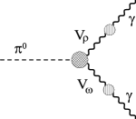
Figure 1: The pion electromagnetic transition amplitude in the large-$N_{c}$ limit.

The large-$Q$ expansion of Eq. (7) would naively yield pure power corrections, assuming a finite number of resonances Moussallam (1995); Knecht and Nyffeler (2001); Ruiz-Femenia et al. (2003). The situation with infinitely many resonances requires some care, since the coefficients of the twist expansion involve positive powers of the meson masses and require regularization. We will illustrate below the situation with an explicit model.

Another, more subtle, question regards the role of radiative corrections in the large-$N_{c}$ limit. This problem also arises in chiral quark models which are specific model realizations of the large-$N_{c}$ limit with explicit quark degrees of freedom Petrov and Pobylitsa (1997); Petrov et al. (1999); Heinzl (2001); Praszalowicz and Rostworowski (2001); Anikin et al. (2001); Dorokhov et al. (2003); Ruiz Arriola and Broniowski (2002, 2003); Ruiz Arriola (2002). We take over the viewpoint adopted in our previous work Ruiz Arriola and Broniowski (2002, 2003); Ruiz Arriola (2002), namely, we consider a situation where all perturbative radiative corrections are switched off. This corresponds to an identification of the power corrections at a given reference scale $Q_{0}$. Thus, our calculations in the large-$N_{c}$ limit determine the initial condition for the QCD evolution, of the form $\varphi_{\pi}^{(n)}(x,Q_{0})$. An obvious advantage of such an approach is that after the evolution the DAs comply to the known asymptotic QCD behavior. We discuss this issue in detail in Sect. IV.

III Large-$N_{c}$ Regge Models

Now we proceed to the basic analysis of this paper, namely a study of Eq. (7) at large $Q^{2}$. The idea is as follows: we adopt a model for the spectra and couplings, calculate the amplitude, and compare to Eq. (5,6). For the spectra we take the radial Regge model

$$M^{2}_{V_{\rho}}(n) = M^{2}_{V_{\omega}}(n)=M^{2}+an,$$ (9)

which assumes for simplicity the same spectra in the $\rho$ and $\omega$ channels. is well fulfilled Anisovich et al. (2000) in the experimentally explored region. We also assume that the $M$ and $a$ parameters are isospin-independent, i.e. are the same for the $\rho$- and $\omega$-type mesons. We investigate possible departures from this assumption later on. We also take constant, i.e. $n$-independent values

$$F_{V_{\rho}} = F_{\rho}={\rm const.},$$

$$F_{V_{\omega}} = F_{\omega}={\rm const.},$$ (10)

as follows from matching of the predictions of the radial Regge model for the vector correlator to QCD Ruiz Arriola and Broniowski (2006). Standard vector-meson dominance yields the relation $F\equiv F_{\rho}=N_{c}F_{\omega}$. The matching yields

$$a=2\pi\sigma=\frac{24\pi^{2}}{N_{c}}F^{2},$$ (11)

where $\sigma$ is the long-distance string tension. If we use $F=154~{}{\rm MeV}$ from the $\rho\to 2\pi$ decay Ecker et al. (1989) we get $\sqrt{\sigma}=546~{}{\rm MeV}$, while the lattice calculation of Ref. Kaczmarek and Zantow (2005) gives a similar order-of-magnitude estimate, $\sqrt{\sigma}=420~{}{\rm MeV}$. Condition (11) originates solely from the asymptotic spectrum and is insensitive to the low-lying states, whose parameters (mass, couplings) may depart form the asymptotic values.

Using the standard Feynman trick we rewrite Eq. (7) in the form

$$F_{\pi^{0}\gamma^{\ast}\gamma^{\ast}}(Q,A)=\sum_{n,n^{\prime}=0}^{\infty}\int_{0}^{1}dx\times$$ (12)

$$\frac{(F^{2}/N_{c})G_{nn^{\prime}}(Q^{2},A)}{\left\{M^{2}+anx+an^{\prime}(1-x)+\frac{1}{2}Q^{2}[1+uA]\right\}^{2}}$$

$$+(A\longleftrightarrow-A),$$

where $G_{nn^{\prime}}$ is the coupling of the pion to the $n$ and $n^{\prime}$ states belonging to the $\rho$ and $\omega$ Regge towers. This coupling may involve diagonal ($n=n^{\prime}$) and non-diagonal ($n\neq n^{\prime}$) terms, hence we introduce $n^{\prime}=n+d$. The double sum may then be transformed into

$$\sum_{n,n^{\prime}=0}^{\infty}A_{nn^{\prime}}=\sum_{d=0}^{\infty}\sum_{m=0}^{\infty}\left(1-\frac{\delta_{0d}}{2}\right)(A_{m,m+d}+A_{m+d,m}),$$

where the factor $(1-{\delta_{0d}}/{2})$ is introduced for the correct counting the the diagonal and non-diagonal terms. On purely physical grounds we expect that the non-diagonal couplings are suppressed, because in that case the radial wave functions involve different number of nodes and the overlap is reduced. Thus it is reasonable to assume that $G_{n,n+d}$ is decreasing sufficiently fast with increasing $d$ such that Eq. (12) makes sense. Note that reasonable as it is, this assumption has sound consequences, as it makes the sum over $n$ and $n^{\prime}$ in Eq. (12) finite. With no suppression the sum diverges logarithmically, however, any power-law suppression of $G_{n,n+d}$ with $d$ makes the expression well-behaved. At asymptotic $Q^{2}$ and fixed $d$ the coupling $G_{n,n+d}$ might a priori depend on $n$. We show, however, that this is impossible, as it would lead to violation of the twist expansion (4). Indeed, assume that $G_{n,n+d}=G_{n+d,n}\sim n^{\alpha(d,Q^{2},A)}g(d,Q^{2},A)$. Then, using the Euler-McLaurin summation formula we can we transform the sum into an integral and get the asymptotic behavior

$$F_{\pi^{0}\gamma^{\ast}\gamma^{\ast}}(Q,A)\sim\sum_{d}\left(1-\frac{\delta_{0d}}{2}\right)\int_{0}^{1}dx\int_{n_{0}}^{\infty}dn$$ (14)

$$\left(\frac{n^{\alpha(d,Q^{2},A)}g(d,Q^{2},A)}{\left\{M^{2}+an+adx+\frac{1}{2}Q^{2}[1+uA]\right\}^{2}}\right.$$

$$\left.+\frac{n^{\alpha(d,Q^{2},A)}g(d,Q^{2},A)}{\left\{M^{2}+an+ad(1-x)+\frac{1}{2}Q^{2}[1+uA]\right\}^{2}}\right)$$

$$\sim\sum_{d}\left(1-\frac{\delta_{0d}}{2}\right)\int_{0}^{1}dx\,g\frac{[1-uA]^{\alpha-1}+[1+uA]^{\alpha-1}}{(Q^{2})^{1-\alpha}},$$

whereas Eqs. (4,5) enforce the leading behavior in the form $1/[Q^{2}(1-u^{2}A^{2})]$. This implies that the only natural way to match to QCD (in the absence of radiative corrections) is to assume that at large $Q^{2}$ and $n$ we have $\alpha=0$ and $g$ depending only on $d$. In other words, the coupling $G_{n,n+d}$ at large $Q^{2}$ and $n$ is independent of $n$, $Q$, and $A$. Thus for simplicity we take $G_{n,n+d}=G_{n+d,n}=g(d)$ for all, even low, $n$. The obtained behavior is reminiscent of the asymptotic independence of the coupling $F_{V}$ of $Q^{2}$ and $n$ in the case of the two-point vector correlator. It is worth stressing that each term in Eq. (12) goes as $1/Q^{4}$ and it is the summation over $n$ which changes the power to $1/Q^{2}$, yielding the leading twist DA properly. Any finite truncation does not do the job. In order to generate the $1/Q^{2}$ behavior one needs the proper asymptotic density of states, such as in the Regge model.

With the formula for the polygamma function,

$$\sum_{n=0}^{\infty}\frac{1}{(u+vn)^{2}}=\frac{1}{v^{2}}\psi^{(1)}\left(\frac{u}{v}\right),$$ (15)

we obtain from Eq. (12) the equation

$$F_{\pi^{0}\gamma^{\ast}\gamma^{\ast}}(Q,A)=\frac{F^{2}}{N_{c}a^{2}}\sum_{d}\left(1-\frac{\delta_{0d}}{2}\right)g(d)\int_{0}^{1}dx\times$$

$$\left[\psi^{(1)}\left(\frac{M^{2}}{a}+dx+\frac{1}{2a}Q^{2}[1+uA]\right)\right.$$ (16)

$$\left.+\psi^{(1)}\left(\frac{M^{2}}{a}+d(1-x)+\frac{1}{2a}Q^{2}[1+uA]\right)\right]$$

$$+(A\longleftrightarrow-A).$$

At large $Q^{2}$ we use the expansion

$$\psi^{(1)}(AQ^{2}+B)=\frac{1}{AQ^{2}}+\left(\frac{1}{2}-B\right)\frac{1}{A^{2}Q^{4}}+\dots$$ (17)

which yields

$$F_{\pi^{0}\gamma^{\ast}\gamma^{\ast}}(Q,A)=\frac{8F^{2}}{N_{c}a}\sum_{d}\left(1-\frac{\delta_{0d}}{2}\right)g(d)\int_{0}^{1}dx\times$$ (18)

$$\left(\frac{1}{Q^{2}(1-u^{2}A^{2})}-\frac{[2M^{2}+a(d-1)](1+u^{2}A^{2})}{Q^{4}(1-u^{2}A^{2})^{2}}+\dots\right).$$

Comparison to Eq. (5,6) gives immediately the identification

$$\varphi^{(2)}(x)=1,\;\;\;\varphi^{(4)}(x)=1,$$ (19)

with the normalization conditions

$$\sum_{d}\left(1-\frac{\delta_{0d}}{2}\right)g(d)=\frac{12\pi^{2}f}{N_{c}},$$ (20)

$$\Delta^{2}=-\frac{N_{c}}{24\pi^{2}f}\sum_{d}\left(1-\frac{\delta_{0d}}{2}\right)g(d)[2M^{2}+a(d-1)]).$$

Note that $g(d)\sim N_{c}^{-1/2}$, as required for 3-meson couplings, and $\Delta^{2}\sim N_{c}^{0}$. The sign of $\Delta^{2}$ is formally not constrained. We stress that the above results hold at the scale $Q_{0}$ at which the radiative gluon corrections are not present.

Let us consider in a greater detail the simplest case where no non-diagonal couplings are present, $g(d)=G\delta_{d0}$. Then Eqs. (20) yield

$$G=\frac{24\pi^{2}f}{N_{c}},\;\;\;\Delta^{2}=\frac{a}{2}-M^{2}.$$ (21)

With $M=m_{\rho}=770$ MeV the parameter $\Delta^{2}$ is positive when $\sqrt{\sigma}>434$ MeV. At $\sqrt{\sigma}=500$ MeV we obtain $\Delta=439$ MeV, which agrees in the order of magnitude with quark-model estimates Anikin et al. (2000b); Ruiz Arriola and Broniowski (2003).

At $Q^{2}=0$ the anomaly condition (8) enforces the relation

$$\psi^{(1)}\left(\frac{m_{\rho}^{2}}{2\pi\sigma}\right)=\frac{\sigma N_{c}}{4\pi f^{2}},$$ (22)

which is very well satisfied for $\sigma=(500~{}{\rm MeV})^{2}$, when the above equation becomes $0.377\simeq 0.377$. If we use the relation $m_{\rho}^{2}=24\pi^{2}f^{2}/N_{c}$, then Eq. (22) becomes $\psi^{(1)}(z)=3/z$, with $z=m_{\rho}^{2}/a\simeq 0.385$, which gives numerically the relation $\sqrt{\sigma}\simeq 0.64m_{\rho}=495$ MeV. This shows that extending the assumption of constancy of the the meson coupling $G$ all the way from the asymptotic region down to $Q^{2}=0$ preserves the constraints of the model. Moreover, it leads to very reasonable results and allows to remarkably well determine the string tension from the meson phenomenology using the chiral anomaly matching condition.

Let us now discuss the effects of modifying the Regge model. Suppose the masses $M$ and the slope parameters $a$ were different in the $\rho$ and $\omega$ channels. If $a_{\rho}\neq a_{\omega}$ then the expansion (5,6) is violated. Note, however, that in that case we would have different asymptotic density of $\rho$ and $\omega$ states, which is not possible in a theory with strict $SU(2)_{F}$ symmetry. On the other hand, it is possible to split $m_{\rho}$ and $m_{\omega}$. In that case still $\varphi^{(2)}=1$, but higher-twist DAs become $x$-dependent. We know from experimental data that the $\omega$-$\rho$ mass splitting is tiny, so that dependence should not be strong. At any case, the result of constant $\varphi^{(2)}$ in the large-$N_{c}$ limit (at the scale $Q_{0}$) seems very robust.

Several comments referring to the interpretation of our results are in order. We recall that the constancy of pion DAs has been originally obtained by the present authors in the Nambu–Jona-Lasinio model Ruiz Arriola and Broniowski (2002) as well as in the Spectral Quark Model Ruiz Arriola and Broniowski (2003), which are particular realizations of the large-$N_{c}$ limit. A key ingredient of these calculation was the correct implementation of chiral symmetry through the Ward-Takahashi identities. On the other hand, calculations based on nonlocal quark models originally obtained bumped distributions Praszalowicz and Rostworowski (2001), close in shape to the asymptotic forms. Later calculations with more careful implementation of PCAC resulted in much flatter results Bzdak and Praszalowicz (2003), with the DA remaining non-zero at the end-points $x=0,1$. The trend to a flat distribution can also be seen in transverse lattice calculations at low transverse scales Dalley (2001); Burkardt and Seal (2002). The present calculation is founded on more general background, using only the facts that at large-$N_{c}$ we deal with a purely mesonic theory and that the confined meson spectrum may be described by the radial Regge model.

Another comment refers to the absence of explicit quarks in the present approach. Interestingly, the calculation, although referring to the partonic structure, as seen in Eq. (1), never explicitly introduces partons of spin 1/2. The $x$ variable enters from the Feynman representation of the product of two vector-meson propagators and is later identified with the Bjorken $x$ by matching to the QCD expressions (5,6). The identification is unique, since DAs are universal for all $Q^{2}$ and $A$ and are only functions of $x$ (and the model parameters).

IV QCD evolution for large and finite $N_{c}$

An important point, not only for our calculation, but for all model calculations, is the question of the energy scale where the obtained predictions for the DAs hold. Distribution amplitudes depend on the scale, while our result corresponds to a fixed reference scale $Q_{0}$. The QCD evolution is crucial, eventually evolving the DAs into their asymptotic forms $\varphi_{\rm as}^{(2)}=6x(1-x)$, $\varphi_{\rm as}^{(4)}=30x^{2}(1-x)^{2}$, …. At leading order the evolution for the leading-twist component is very simple. One method is to use the Gegenbauer moments (see Appendix A), which evolve with the evolution ratio $[\alpha(Q^{2})/\alpha(Q_{0}^{2})]^{\gamma_{n}^{(0)}/2\beta_{0}}$. Since $\beta_{0}=11N_{c}/3-2N_{f}/3$, and $\gamma_{n}^{(0)}\sim(N_{c}^{2}-1)/(2N_{c})$ the exponent reaches a finite value in the large-$N_{c}$ limit. As expected, the quark contribution (depending on the number of active flavors $N_{F}$) is only $1/N_{c}$ suppressed. For instance, the second Gegenbauer moment behaves as

$$\frac{a_{2}(Q)}{a_{2}(Q_{0})}=\left(\frac{\alpha(Q)}{\alpha(Q_{0})}\right)^{\frac{75(N_{c}^{2}-1)}{12N_{c}(11N_{c}-2N_{F})}}$$ (23)

From the present calculation one gets $a_{2}(Q_{0})=7/18$. For $N_{F}=3$ the exponent changes from $50/81$ at $N_{c}=3$ to $25/44$ at $N_{c}=\infty$, an effect at the $10\%$ level only. Thus, the (perturbative) evolution is never switched off. Obviously, our result for the DA cannot hold at all scales. As we said, it refers to a particular reference scale $Q_{0}$. It is precisely at that situation where the DAs are constant functions of $x$. In order to pass to other scales, the evolution is necessary and its effect is strong. In particular, the evolution changes the end-point behavior near $x=0,1$, for instance the twist-2 component $\varphi^{(2)}\sim x$ near $x=0$ and $\varphi^{(2)}\sim 1-x$ near $x=1$ (see Refs. Ruiz Arriola and Broniowski (2002) for details). This effect is very important, in particular for the analysis of processes with one real photon, where $A=1$. Then the numerators in integrands of Eq. (5,6) involve powers of $x(1-x)$ and the transition form factor is well-behaved only when the end-point behavior of the DA cancels the singularity. In short, the QCD evolution is mandatory if we want to compare the model predictions to the data.

Having said that, we note that we can compute exactly the unevolved large-$N_{c}$ pion transition form factor, which amounts to carrying the $x$ integration in Eq. (16). For the diagonal model, $g(d)=G\delta_{d0}$, we find

$$F_{\pi^{0}\gamma^{\ast}\gamma^{\ast}}(Q,A) = \frac{2f}{N_{c}AQ^{2}}\left[\psi^{(0)}\left(\frac{M^{2}}{a}+\frac{Q^{2}(1+A)}{2a}\right)\right.$$ (24)

$$\left.-\psi^{(0)}\left(\frac{M^{2}}{a}+\frac{Q^{2}(1-A)}{2a}\right)\right].$$

Figure 2: The pion transition form factor in the large-$N_{c}$ Regge model. Solid lines from top to bottom correspond to Eq. (24) at $|A|=1$, $0.95$, $0.75$, $0.5$, and $0$, respectively. The dashed lines indicate the Brodsky-Lepage limit of $2f$ for $|A|=1$ (upper curve) and $4f/3$ for $|A|=0$ (lower curve). The CLEO data points are for $A=1$.

This result is plotted for different values of the asymmetry $A$ in Fig. 2, where the need for evolution at large $Q^{2}$ is vividly seen. The top curve (thick line) is for the un-evolved large-$N_{c}$ result of Eq. (24) with $A=1$. At large-$Q^{2}$ we have

$$Q^{2}F_{\pi^{0}\gamma^{\ast}\gamma}(Q,|A|=1) = \frac{2f}{N_{c}}\left[\log\frac{Q^{2}}{a}+\psi^{(0)}\left(\frac{M^{2}}{a}\right)\right]$$ (25)

$$+{\cal O}(1/Q^{2}).$$

We note the $\log Q^{2}$ term, whose presence can be traced back to the singular end-point behavior in the twist expansion (4-6). As a result, the pure twist expansion is violated. The QCD evolution cures this problem, leading to the asymptotic behavior in accordance to the Brodsky-Lepage limit, indicated with the upper dashed line in Fig. 2. Therefore the QCD evolution is necessary to comply to the formal limit, as well as to the experimental data. More pictorially, the evolution takes the tail of the model calculation and brings it down to the upper dashed line, compatible with the data. We stress again that the data should not be directly compared to the un-evolved model results plotted in the figure, yet we notice that at lower $Q^{2}$, where the effects of evolution should be smaller, the comparison is quite reasonable. At lower values of $|A|$ the effects of evolution are not as strong as at $|A|=1$, moreover, the pure twist expansion (i.e. the expansion in powers of $1/Q^{2}$ without logs) holds. In the symmetric limit of $A=0$ we have

$$F_{\pi^{0}\gamma^{\ast}\gamma^{\ast}}(Q,A=0)=\frac{2f}{N_{c}a}\psi^{(1)}\left(\frac{2M^{2}+Q^{2}}{2a}\right).$$ (26)

Finally, let us mention that the determination of the reference scale $Q_{0}$ can only be done at present using perturbative evolution. In our previous work Ruiz Arriola and Broniowski (2002) we used the second Gegenbauer moment $a_{2}=0.12\pm 0.03$ at $Q=2.4~{}{\rm GeV}$ extracted from the experiment Schmedding and Yakovlev (2000) with the assumption $a_{k}=0$ for $k>2$. This allowed us to make the LO estimate for the evolution ratio $\alpha(Q)/\alpha(Q_{0})=0.15\pm 0.06$. In Fig. 3 we show the corresponding LO Gegenbauer evolution for $N_{c}=3$ and $N_{c}=\infty$ to the scale $Q^{2}=5.8~{}{\rm GeV}^{2}$. As we see the $N_{c}$-effect is tiny and is in fact comparable with the uncertainties induced by the evolution ratio Ruiz Arriola and Broniowski (2002). Let us note that despite the perturbative nature of our evolution the similarity of these evolved results to non-perturbative transverse lattice calculations with a transverse lattice size of about $a_{\perp}\sim 0.5-0.7~{}{\rm fm}$ is indeed striking . The LO reference scale of our estimate turns out to be $Q_{0}=0.320\pm 0.045~{}{\rm GeV}$ (for $\Lambda_{\rm QCD}=0.224~{}{\rm GeV}$) – a rather low value which suggests the usage of higher-order evolution Mueller (1995) or even non-perturbative evolution Dalley (2001); Burkardt and Seal (2002). Our constant DA evolved at LO to the CLEO scale $Q^{2}=5.8~{}{\rm GeV}^{2}$ yields the value $Q^{2}F_{\gamma^{*},\pi\gamma}(Q)/(2f_{\pi})=1.25\pm 0.10$  Ruiz Arriola and Broniowski (2002), higher but compatible within two standard deviations to the experimental CLEO value of $0.83\pm 0.12$. This actually speaks in favor of small NLO corrections, however work on higher-order evolution should definitely be pursued in the future. In addition, the higher twist corrections should also be included in such an analysis, which is nontrivial.

Expansion of Eq. (24) at low-$Q^{2}$ yields

$$F_{\pi^{0}\gamma^{\ast}\gamma^{\ast}}(Q,A) = \frac{2f}{3a}\psi^{(1)}\left(\frac{M^{2}}{a}\right)+\frac{fQ^{2}}{3a^{2}}\psi^{(2)}\left(\frac{M^{2}}{a}\right)$$ (27)

$$+ \frac{f(A^{2}+3)Q^{4}}{36a^{3}}\psi^{(3)}\left(\frac{M^{2}}{a}\right)+\dots$$

Note that the $Q^{2}$ term is independent of the asymmetry $A$, as is also apparent from Fig. 2. The corresponding slope reads

$$b_{\pi} = -\left[\frac{1}{F_{\pi^{0}\gamma\gamma^{\ast}}(Q,0)}\frac{d}{dQ^{2}}F_{\pi^{0}\gamma\gamma^{\ast}}(Q,0)\right]\Big{|}_{Q^{2}=0}$$ (28)

$$= -\frac{1}{2a}\frac{\psi^{(2)}\left(\frac{M^{2}}{a}\right)}{\psi^{(1)}\left(\frac{M^{2}}{a}\right)}$$

Numerically, taking $M=m_{\rho}=770$ MeV we get the value $b_{\pi}=1.39~{}{\rm GeV}^{-2}$ for $\sigma=(400~{}{\rm MeV})^{2}$, $b_{\pi}=1.51~{}{\rm GeV}^{-2}$ for $\sigma=(500~{}{\rm MeV})^{2}$, and $b_{\pi}=1.58~{}{\rm GeV}^{-2}$ for $\sigma=(600~{}{\rm MeV})^{2}$. These Regge model estimates are in very reasonable agreement with the experimental values quoted in the PDG Eidelman et al. (2004): $b_{\pi}=(1.79\pm 0.14\pm 14){\rm GeV}^{-2}$ originally reported by the CELLO collaboration Behrend et al. (1991), obtained from an extrapolation from high-$Q^{2}$ data to low $Q^{2}$ by means of generalized vector meson dominance, $b_{\pi}=(1.4\pm 1.3\pm 2.6){\rm GeV}^{-2}$ given in Farzanpay et al. (1992), and $b_{\pi}=(1.4\pm 0.8\pm 1.4){\rm GeV}^{-2}$ given in Meijer Drees et al. (1992).

Finally, let us comment on the recent findings within the holographic approach Brodsky and de Teramond (2006b, a) where the light-cone wave functions have been computed appealing to the AdS/CFT correspondence and the meromorpization approach of Ref. Radyushkin (2006). The holographic wave-functions correspond to a spectrum which behaves linearly in the mass, $M(n)\sim n$. Based on a conformal-based mapping Brodsky and Teramond Brodsky and de Teramond (2006b) get the asymptotic DA $\varphi_{\pi}^{(2)}(x)=6x(1-x)$ while the corresponding Parton Distribution Function (PDF) is $f_{\pi}(x)=6x(1-x)$. If, instead, a twist-based mapping is considered Brodsky and de Teramond (2006a) these authors get $\varphi_{\pi}^{(2)}(x)=(8/\pi)\sqrt{x(1-x)}$ and a PDF $f_{\pi}(x)=1$. According to the meromorphization approach of Radyushkin Radyushkin (2006) one gets $\varphi_{\pi}^{(2)}(x)=(8/\pi)\sqrt{x(1-x)}$ and $f_{\pi}(x)=1$ for scalar quarks and $\varphi_{\pi}^{(2)}(x)=6x(1-x)$ , the asymptotic DA, and $f_{\pi}(x)=6x(1-x)$ for spin 1/2 quarks. This latter situation is exactly the kind of situation that was found in the NJL quantized on the light cone Heinzl (2001). An asymptotic PDA suggests a reference scale $Q_{0}=\infty$ or the lack of LO evolution of $\phi^{2}$, which assumes the asymptotic form at all scales. On the other hand the corresponding PDF yields a $100\%$ momentum fraction carried by the quarks, while for $Q_{0}=\infty$ one expects that all momentum fraction is carried by the gluons. This poses an interpretation difficulty for these approaches which should be cleared out.

Figure 3: The pion distribution amplitude evolved to the scale $Q^{2}=(2.4{\rm GeV})^{2}$ for the cases $N_{c}=3$ and $N_{c}=\infty$. The value for the evolution ratio $\alpha(Q)/\alpha(Q_{0})=0.15$ is based on the analysis of the CLEO data of Ref. Schmedding and Yakovlev (2000). We also show the un-evolved DA, $\varphi_{\pi}(x,Q_{0})=1$, and the asymptotic DA, $\varphi_{\pi}(x,\infty)=6x(1-x)$.

V Conclusion

We summarize our main points. The radial Regge model predictions for the $\pi^{0}\gamma^{\ast}\gamma^{\ast}$ amplitude can be matched to the QCD twist expansion in the absence of radiative corrections in the large-$N_{c}$ limit. The matching requires that the coupling of the pion to a pair of Regge $\rho$ and $\omega$ mesons, $G_{\pi VV^{\prime}}$, is constant for highly excited Regge states and large momenta. The twist-2 pion distribution amplitude is then found to be constant in the $x$-variable, conforming to the earlier predictions made in a class of chiral quark models. Thus, we provide an explicit example of quark-hadron duality for an exclusive process. Moreover, higher-twist DAs may or may not be constant, depending on the details of the Regge model. If $m_{\rho}=m_{\omega}$, then the twist-4 DA is also constant. The Regge model couplings are constrained by matching the chiral anomaly for real photons and the high-momentum behavior, cf. Eqs. (20,21) for highly virtual photons. If we further assume a model with constant diagonal couplings, a consistency relation (22) involving the string tension is found, which is well supported by the data. As a result the string tension is found to scale with the square of the $\rho$-meson mass. The Regge model results is very reasonable predictions for the slope of the pion electromagnetic transition form factor at zero momentum. The estimates depend weakly on the string tension, and compare quite well to the existent measurements. Finally, we have noted that similarly to the case of chiral quark models, the QCD evolution is necessary in the present Regge model to achieve the correct large-momentum behavior of the pion transition form factor.

Appendix A LO evolution of DA

The LO-evolved distribution amplitude reads Lepage and Brodsky (1980); Mueller (1995)

$$\varphi_{\pi}^{(2)}(x,Q) = 6x(1-x){\sum_{n=0}^{\infty}}^{\prime}C_{n}^{3/2}(2x-1)a_{n}(Q),$$ (29)

where the prime indicates summation over even values of $n$ only. The matrix elements, $a_{n}(Q)$, are the Gegenbauer moments given by

$$a_{n}(Q) = \frac{2}{3}\frac{2n+3}{(n+1)(n+2)}\left(\frac{\alpha(Q)}{\alpha(Q_{0})}\right)^{\gamma_{n}^{(0)}/(2\beta_{0})}\times$$ (30)

$$\int_{0}^{1}dxC_{n}^{3/2}(2x-1)\varphi_{\pi}^{(2)}(x,Q_{0}),$$

with $C_{n}^{3/2}$ denoting the Gegenbauer polynomials, and the non-singlet anomalous dimension reads

$$\gamma_{n}^{(0)} = -2C_{F}\left[3+\frac{2}{(n+1)(n+2)}-4\sum_{k=1}^{n+1}\frac{1}{k}\right],$$

$$\beta_{0} = \frac{11}{3}C_{A}-\frac{2}{3}N_{F},$$ (31)

with $C_{A}=N_{c}$, $C_{F}=(N_{c}^{2}-1)/(2N_{c})$, and $N_{F}$ being the number of active flavors, which we take equal to three. The LO running is then $\alpha(Q)=(4\pi/\beta_{0})/\log(Q^{2}/\Lambda_{\rm QCD}^{2})$. Taking as initial condition

$$\varphi_{\pi}^{(2)}(x,Q_{0})=1\,,$$ (32)

one we gets immediately

$$a_{n}(Q) = \frac{2}{3}\frac{2n+3}{(n+1)(n+2)}\left(\frac{\alpha(Q)}{\alpha(Q_{0})}\right)^{\gamma_{n}^{(0)}/(2\beta_{0})}\,.$$ (33)

References

- Lepage and Brodsky (1980) G. P. Lepage and S. J. Brodsky, Phys. Rev. D22, 2157 (1980).
- Chernyak and Zhitnitsky (1984) V. L. Chernyak and A. R. Zhitnitsky, Phys. Rept. 112, 173 (1984).
- Dittes and Radyushkin (1981) F. M. Dittes and A. V. Radyushkin, Sov. J. Nucl. Phys. 34, 293 (1981).
- Mueller (1995) D. Mueller, Phys. Rev. D51, 3855 (1995), eprint hep-ph/9411338.
- Braun et al. (2003) V. M. Braun, G. P. Korchemsky, and D. Mueller, Prog. Part. Nucl. Phys. 51, 311 (2003), eprint hep-ph/0306057.
- Dalley (2001) S. Dalley, Phys. Rev. D64, 036006 (2001), eprint hep-ph/0101318.
- Burkardt and Seal (2002) M. Burkardt and S. K. Seal, Phys. Rev. D65, 034501 (2002), eprint hep-ph/0102245.
- Burkardt and Dalley (2002) M. Burkardt and S. Dalley, Prog. Part. Nucl. Phys. 48, 317 (2002), eprint hep-ph/0112007.
- Del Debbio et al. (2003) L. Del Debbio, M. Di Pierro, and A. Dougall, Nucl. Phys. Proc. Suppl. 119, 416 (2003), eprint hep-lat/0211037.
- Del Debbio (2005) L. Del Debbio, Few Body Syst. 36, 77 (2005).
- Gockeler et al. (2005) M. Gockeler et al. (2005), eprint hep-lat/0510089.
- Belyaev and Johnson (1997) V. M. Belyaev and M. B. Johnson, Phys. Rev. D56, 1481 (1997), eprint hep-ph/9702207.
- Behrend et al. (1991) H. J. Behrend et al. (CELLO), Z. Phys. C49, 401 (1991).
- Gronberg et al. (1998) J. Gronberg et al. (CLEO), Phys. Rev. D57, 33 (1998), eprint hep-ex/9707031.
- Schmedding and Yakovlev (2000) A. Schmedding and O. I. Yakovlev, Phys. Rev. D62, 116002 (2000), eprint hep-ph/9905392.
- Bakulev et al. (2001) A. P. Bakulev, S. V. Mikhailov, and N. G. Stefanis, Phys. Lett. B508, 279 (2001), eprint hep-ph/0103119.
- Bakulev et al. (2003) A. P. Bakulev, S. V. Mikhailov, and N. G. Stefanis, Phys. Rev. D67, 074012 (2003), eprint hep-ph/0212250.
- Bakulev et al. (2004a) A. P. Bakulev, S. V. Mikhailov, and N. G. Stefanis, Phys. Lett. B578, 91 (2004a), eprint hep-ph/0303039.
- Bakulev et al. (2006) A. P. Bakulev, S. V. Mikhailov, and N. G. Stefanis, Phys. Rev. D73, 056002 (2006), eprint hep-ph/0512119.
- Agaev (2005) S. S. Agaev, Phys. Rev. D72, 114010 (2005), eprint hep-ph/0511192.
- Aitala et al. (2001) E. M. Aitala et al. (E791), Phys. Rev. Lett. 86, 4768 (2001), eprint hep-ex/0010043.
- Bakulev et al. (2004b) A. P. Bakulev, S. V. Mikhailov, and N. G. Stefanis, Annalen Phys. 13, 629 (2004b), eprint hep-ph/0410138.
- ’t Hooft (1974) G. ’t Hooft, Nucl. Phys. B72, 461 (1974).
- Witten (1979) E. Witten, Nucl. Phys. B160, 57 (1979).
- Petrov and Pobylitsa (1997) V. Y. Petrov and P. V. Pobylitsa (1997), eprint hep-ph/9712203.
- Petrov et al. (1999) V. Y. Petrov, M. V. Polyakov, R. Ruskov, C. Weiss, and K. Goeke, Phys. Rev. D59, 114018 (1999), eprint hep-ph/9807229.
- Heinzl (2001) T. Heinzl, Lect. Notes Phys. 572, 55 (2001), eprint hep-th/0008096.
- Praszalowicz and Rostworowski (2001) M. Praszalowicz and A. Rostworowski, Phys. Rev. D64, 074003 (2001), eprint hep-ph/0105188.
- Anikin et al. (2001) I. V. Anikin, A. E. Dorokhov, and L. Tomio, Phys. Atom. Nucl. 64, 1329 (2001).
- Anikin et al. (2000a) I. V. Anikin, A. E. Dorokhov, and L. Tomio, Phys. Part. Nucl. 31, 509 (2000a).
- Dorokhov et al. (2003) A. E. Dorokhov, M. K. Volkov, and V. L. Yudichev, Phys. Atom. Nucl. 66, 941 (2003), eprint hep-ph/0203136.
- Dorokhov (2003) A. E. Dorokhov, JETP Lett. 77, 63 (2003), eprint hep-ph/0212156.
- Ruiz Arriola and Broniowski (2002) E. Ruiz Arriola and W. Broniowski, Phys. Rev. D66, 094016 (2002), eprint hep-ph/0207266.
- Ruiz Arriola and Broniowski (2003) E. Ruiz Arriola and W. Broniowski, Phys. Rev. D67, 074021 (2003), eprint hep-ph/0301202.
- Ruiz Arriola (2002) E. Ruiz Arriola, Acta Phys. Polon. B33, 4443 (2002), eprint hep-ph/0210007.
- Bzdak and Praszalowicz (2003) A. Bzdak and M. Praszalowicz, Acta Phys. Polon. B34, 3401 (2003), eprint hep-ph/0305217.
- Anisovich et al. (2000) A. V. Anisovich, V. V. Anisovich, and A. V. Sarantsev, Phys. Rev. D62, 051502 (2000), eprint hep-ph/0003113.
- Golterman and Peris (2001) M. Golterman and S. Peris, JHEP 01, 028 (2001), eprint hep-ph/0101098.
- Simonov (2002) Y. A. Simonov, Phys. Atom. Nucl. 65, 135 (2002), eprint hep-ph/0109081.
- Golterman and Peris (2003) M. Golterman and S. Peris, Phys. Rev. D67, 096001 (2003), eprint hep-ph/0207060.
- Afonin et al. (2004) S. S. Afonin, A. A. Andrianov, V. A. Andrianov, and D. Espriu, JHEP 04, 039 (2004), eprint hep-ph/0403268.
- Afonin and Espriu (2006) S. S. Afonin and D. Espriu (2006), eprint hep-ph/0602219.
- Ruiz Arriola and Broniowski (2006) E. Ruiz Arriola and W. Broniowski (2006), eprint hep-ph/0603263.
- Moussallam (1995) B. Moussallam, Phys. Rev. D51, 4939 (1995), eprint hep-ph/9407402.
- Knecht and Nyffeler (2001) M. Knecht and A. Nyffeler, Eur. Phys. J. C21, 659 (2001), eprint hep-ph/0106034.
- Beane (2001a) S. R. Beane, Phys. Rev. D64, 116010 (2001a), eprint hep-ph/0106022.
- Beane (2001b) S. R. Beane, Phys. Lett. B521, 47 (2001b), eprint hep-ph/0108025.
- Ruiz-Femenia et al. (2003) P. D. Ruiz-Femenia, A. Pich, and J. Portoles, JHEP 07, 003 (2003), eprint hep-ph/0306157.
- Dominguez (2001) C. A. Dominguez, Phys. Lett. B512, 331 (2001), eprint hep-ph/0102190.
- Dominguez and Thapedi (2004) C. A. Dominguez and T. Thapedi, JHEP 10, 003 (2004), eprint hep-ph/0409111.
- Radyushkin (1995) A. V. Radyushkin, Acta Phys. Polon. B26, 2067 (1995), eprint hep-ph/9511272.
- Brodsky and de Teramond (2006a) S. J. Brodsky and G. F. de Teramond, Phys. Rev. Lett. 96, 201601 (2006a), eprint hep-ph/0602252.
- Brodsky and de Teramond (2006b) S. J. Brodsky and G. F. de Teramond, Int. J. Mod. Phys. A21, 762 (2006b), eprint hep-ph/0509269.
- Radyushkin (2006) A. V. Radyushkin (2006), eprint hep-ph/0605116.
- Ecker et al. (1989) G. Ecker, J. Gasser, A. Pich, and E. de Rafael, Nucl. Phys. B321, 311 (1989).
- Kaczmarek and Zantow (2005) O. Kaczmarek and F. Zantow, Phys. Rev. D71, 114510 (2005), eprint hep-lat/0503017.
- Anikin et al. (2000b) I. V. Anikin, A. E. Dorokhov, and L. Tomio, Phys. Lett. B475, 361 (2000b), eprint hep-ph/9909368.
- Eidelman et al. (2004) S. Eidelman, K. Hayes, K. Olive, M. Aguilar-Benitez, C. Amsler, D. Asner, K. Babu, R. Barnett, J. Beringer, P. Burchat, et al., Physics Letters B 592, 1+ (2004), URL http://pdg.lbl.gov.
- Farzanpay et al. (1992) F. Farzanpay et al., Phys. Lett. B278, 413 (1992).
- Meijer Drees et al. (1992) R. Meijer Drees et al. (SINDRUM-I), Phys. Rev. D45, 1439 (1992).