DESY 06-072

hep-ph/0605297

August, 2006

The Gravitino-Overproduction Problem in Inflationary Universe
Masahiro Kawasaki¹, Fuminobu Takahashi^1,2 and T. T. Yanagida^3,4

¹Institute for Cosmic Ray Research, University of Tokyo,
Chiba 277-8582, Japan
²Deutsches Elektronen Synchrotron DESY, Notkestrasse 85,
22607 Hamburg, Germany
³Department of Physics, University of Tokyo,
Tokyo 113-0033, Japan
⁴Research Center for the Early Universe, University of Tokyo,
Tokyo 113-0033, Japan

1 Introduction

The gravitino is the most important prediction of unified theory of quantum mechanics and general relativity such as the superstring theory (i.e. supergravity (SUGRA) at low energies) [1]. However, the presence of the gravitino leads to serious cosmological problems depending on its mass and nature. If the gravitino is unstable and has a mass $m_{3/2}$ in the range from $O(100)$ GeV to $O(10)$ TeV, the decay of the gravitino destroys light elements produced by the big-bang nucleosynthesis (BBN). To keep the success of BBN the reheating temperature $T_{R}$ after inflation should be lower than $O(10^{6-8})$ GeV suppressing the gravitino production by thermal scattering. On the other hand, if the gravitino is light as $m_{3/2}<O(10)$ GeV and it is stable (that is, the lightest supersymmetric particle (LSP)), the reheating temperature should satisfy $T_{R}\mathop{}_{\textstyle\sim}^{\textstyle<}O(10^{7}){\rm\,GeV}(m_{3/2}/1{\rm\,GeV})$ for $m_{3/2}\mathop{}_{\textstyle\sim}^{\textstyle>}100$ keV for the gravitino density not to exceed the observed dark matter density.

In a recent article [2], we have pointed out that there is a new gravitino problem beside due to the thermal production of the gravitino. That is, an inflaton field $\phi$ has nonvanishing supersymmetry(SUSY)-breaking auxiliary field $G_{\phi}$ (or more precisely ${\cal G}^{\rm(eff)}_{\Phi}$ as will be defined later) in most of inflation models in SUGRA, which gives rise to an enhanced decay of the inflaton into a pair of gravitinos, if the Kähler potential is non-minimal. Thus, we have stringent constraints on the (effective) auxiliary field ${\cal G}^{\rm(eff)}_{\Phi}$ to suppress the production of gravitinos in the inflaton decay [2]. This gravitino production in inflaton decay is more effective for lower reheating temperature, while the production by particle scatterings in the thermal bath is more important for higher temperature $T_{R}$. Therefore, the direct gravitino production discussed in this paper is complementary to the thermal gravitino production, and the former may put severe constraints on inflation models together with the latter.

The purpose of this paper is to discuss this new gravitino problem in a broad mass range of the gravitino including $m_{3/2}\simeq O(100)$TeV region suggested from anomaly-mediated SUSY breaking models [3]. We assume, in the present analysis, that there is no entropy production after the end of reheating by the inflaton decay. However, we briefly discuss, in the last section of this paper, the case that a late-time entropy production takes place.

In Sec. 2 we briefly review the gravitino problem in cosmology and in Sec. 3 we calculate the abundance of gravitinos produced by particle scatterings in the thermal bath and show cosmological constraints on the reheating temperature $T_{R}$. In Sec. 4 we discuss the enhanced decay of the inflaton into a pair of gravitinos and give cosmological constraints on the (effective) auxiliary field ${\cal G}^{\rm(eff)}_{\Phi}$. In Sec. 5 we explicitly calculate the precise value of ${\cal G}^{\rm(eff)}_{\Phi}$ for inflation models in SUGRA to demonstrate how severe the new constraints are. The last section is devoted to conclusions.

2 Gravitino problem

The gravitino is the SUSY partner of the graviton in SUGRA and it acquires a mass in a range of ${\cal O}(100)\ {\rm GeV}-{\cal O}(10)$ TeV in gravity-mediated SUSY-breaking models . Such a gravitino is likely unstable and its lifetime is very long because interactions of the gravitino are suppressed by inverse powers of the reduced Planck scale $M_{P}$. The gravitino dominantly decays into the standard-model (SM) particles and their superpartners, which may produce a large entropy and destroy the light elements synthesized in BBN. As a result, the predictions of BBN may be significantly changed unless the primordial abundance of the gravitino is sufficiently small [6].

In gauge-mediated SUSY-breaking models [7], the gravitino is light ($m_{3/2}\mathop{}_{\textstyle\sim}^{\textstyle<}10$ GeV) and stable. In this case the gravitino may give too much contribution to the present cosmic density of the universe.

In the inflationary universe, the primordial gravitino is once diluted but it is produced during reheating epoch after the inflation. Thus, even in the inflationary models, we may still have the gravitino problem [8]. As shown in the next section, this leads to very stringent constraints on the reheating temperature $T_{R}$ since the gravitino abundance is approximately proportional to $T_{R}$. The constraints are given in [9, 10, 11, 12, 13, 14, 15, 16] for the unstable gravitino and in [17] for the stable one.

3 Thermal production of gravitinos and cosmological constraints on the reheating temperature $T_{R}$

In this section we show the abundance of the gravitinos thermally produced after inflation and derive constraints on the reheating temperature.

During reheating the gravitino is produced through scatterings of particles in thermal bath. The interactions of the gravitino with a gauge multiplet ($A_{\mu},\lambda$) and a chiral multiplet ($\eta,\chi$) are described by

$${\cal L} = -\frac{1}{\sqrt{2}M_{P}}D_{\nu}\eta^{\dagger}\bar{\psi}_{\mu}\gamma^{\nu}\gamma^{\mu}\chi_{R}-\frac{1}{\sqrt{2}M_{P}}D_{\nu}\eta\bar{\chi}_{L}\gamma^{\mu}\gamma^{\nu}\psi_{\mu}$$ (1)

$$-\frac{i}{8M_{P}}\bar{\psi}_{\mu}\left[\gamma^{\nu},\gamma^{\rho}\right]\gamma^{\mu}\lambda F_{\nu\rho},$$

where $F_{\nu\rho}$ is the field strength of the gauge field. (Here, $D_{\nu}$ denotes the covariant derivative and $\chi_{R}$ satisfies $(1-\gamma_{5})\chi_{R}=0$.) The thermally averaged cross section of the gravitino production for an $SU(N)$ super Yang-Mills model with $n_{\rm f}$ pairs of fundamental and anti-fundamental chiral superfields is calculated in Ref. [18] as

$$\langle\sigma v_{\rm rel}\rangle = \left[1+\left(\frac{m_{\tilde{g}}^{2}}{3m_{3/2}^{2}}\right)\right]\frac{3g^{2}(N^{2}-1)}{32\pi M_{P}^{2}}$$ (2)

$$\times\frac{\pi^{2}}{\zeta(3)}\left\{\left[\ln(T^{2}/m_{g,{\rm th}}^{2})+0.3224\right](N+n_{\rm f})+0.5781n_{\rm f}\right\},$$

where $m_{\tilde{g}}$ is the gaugino mass and $m_{g,{\rm th}}$ is the thermal mass of the gauge boson which is given as $m_{g,{\rm th}}^{2}=(1/6)g^{2}(N+n_{\rm f})T^{2}$.

Solving the Boltzmann equation with the above cross section, one can obtain the gravitino-to-entropy ratio $Y_{3/2}$ which is well approximated by [19]

$$Y_{3/2} \simeq 1.9\times 10^{-12}\left[1+\left(\frac{m_{\tilde{g}_{3}}^{2}}{3m_{3/2}^{2}}\right)\right]\left(\frac{T_{\rm R}}{10^{10}\ {\rm GeV}}\right)$$ (3)

$$\times \left[1+0.045\ln\left(\frac{T_{\rm R}}{10^{10}\ {\rm GeV}}\right)\right]\left[1-0.028\ln\left(\frac{T_{\rm R}}{10^{10}\ {\rm GeV}},\right)\right],$$

where we have taken $N=3$ for QCD and $m_{\tilde{g}_{3}}$ is the gluino mass evaluated at $T=T_{R}$. Notice that the gravitino abundance is roughly proportional to $T_{R}$.

For the gravitino of a relatively large mass $\mathop{}_{\textstyle\sim}^{\textstyle>}100$ GeV, it likely decays to the SM particles and their superpartners. In that case, high energy photons and hadrons emitted in the gravitino decay may destroy the light elements (D,³He, ⁴He, ⁷Li, $\cdots$) and hence spoil the success of BBN. Since the gravitino abundance is approximately proportional to $T_{R}$, we obtain an upper bound on the reheating temperature after inflation.

Energetic photons from the radiative decay of gravitino ($\psi_{\mu}\rightarrow\gamma+\tilde{\gamma}$) deconstruct D, which gives an upper bound $T_{R}\mathop{}_{\textstyle\sim}^{\textstyle<}10^{9}$ GeV for $m_{3/2}\simeq 1-3$ TeV. They also cause an overcreation of ³He due to photo-dissociation of ⁴He, which leads to the most stringent constraint on $T_{R}$ as $T_{R}\simeq 10^{6}-10^{9}$ GeV for $m_{3/2}\simeq 100$ GeV $-1$ TeV.

However, it was found in Ref. [19] that the hadronic decay gives a more stringent constraint on the abundance of gravitinos and equivalently on the reheating temperature $T_{R}$ because mesons and nucleons produced in the decay and subsequent hadronization processes significantly affect BBN. In particular, when the branching ratio into hadrons is $\sim 1$ as expected for the gravitino decaying into gluino and gluon, the effect of the hadronic decay is much more serious than the radiative one.

In the case of $B_{h}=1$ ($B_{h}$: the branching ratio of the hadronic decay), the upper bound on $T_{R}$ for relatively light gravitino $m_{3/2}\simeq 0.1-0.2$ TeV comes from the overproduction of ³He as

$$T_{R}~{}\mathop{}_{\textstyle\sim}^{\textstyle<}~{}(1-4)\times 10^{6}~{}{\rm GeV}~{}~{}~{}~{}~{}~{}~{}{\rm for}~{}~{}m_{3/2}\simeq 0.1-0.2~{}{\rm TeV}~{}~{}~{}~{}(B_{h}\simeq 1),$$ (4)

Here we conservatively assume $m_{\tilde{g}}\ll m_{3/2}$. For $m_{3/2}\simeq 0.2-1$ TeV, non-thermal production of ⁶Li sets the very stringent constraint as,

$$T_{R}~{}\mathop{}_{\textstyle\sim}^{\textstyle<}~{}3\times 10^{5}-4\times 10^{6}~{}{\rm GeV}~{}~{}~{}~{}{\rm for}~{}~{}m_{3/2}\simeq 0.2-2~{}{\rm TeV}~{}~{}~{}~{}(B_{h}\simeq 1).$$ (5)

For larger gravitino mass the destruction of D gives the stringent constraint,

$$T_{R}~{}\mathop{}_{\textstyle\sim}^{\textstyle<}~{}5\times 10^{5}-1\times 10^{8}~{}{\rm GeV}~{}~{}~{}~{}{\rm for}~{}~{}m_{3/2}\simeq 2-10~{}{\rm TeV}~{}~{}~{}~{}(B_{h}\simeq 1).$$ (6)

Since the gravitino of mass larger than 10 TeV decays before the light elements are synthesized, the stringent constraint is not obtained from hadro-dissociation processes. However, the mesons (mainly pions) produced at $\sim 1~{}\sec$ alter the proton-neutron ratio and increase the abundance of ⁴He, from which the upper bound on $T_{R}$ is obtained as

$$T_{R}~{}\mathop{}_{\textstyle\sim}^{\textstyle<}~{}(3-10)\times 10^{9}~{}{\rm GeV}~{}~{}~{}~{}{\rm for}~{}~{}m_{3/2}\simeq 10-30~{}{\rm TeV}.~{}~{}~{}~{}(B_{h}\simeq 1)$$ (7)

For $m_{3/2}\mathop{}_{\textstyle\sim}^{\textstyle>}30$ TeV the gravitino decay little affects BBN in the case of $B_{h}=1$.

When the main decay mode is not hadronic, the above constraints become milder. However, even if the gravitino dominantly decays into a photon and a photino, the hadronic branching ratio is non-vanishing since the quark-anti-quark pair can be attached at the end of the virtual photon line. In this case, $B_{h}$ is expected to be of order ${\cal O}(\alpha_{\rm em}/4\pi)\simeq 10^{-3}$. Even such small $B_{h}$ makes the constraint severer than that for pure radiative decay ($B_{h}=0$) as

$$T_{R}~{}\mathop{}_{\textstyle\sim}^{\textstyle<}~{}1\times 10^{6}-3\times 10^{8}~{}{\rm GeV}~{}~{}~{}~{} {\rm for} ~{}~{}m_{3/2}\simeq 0.1-1~{}{\rm TeV}$$ (8)

$$T_{R}~{}\mathop{}_{\textstyle\sim}^{\textstyle<}~{}1\times 10^{8}-3\times 10^{8}~{}{\rm GeV}~{}~{}~{}~{} {\rm for} ~{}~{}m_{3/2}\simeq 1-3~{}{\rm TeV}$$ (9)

$$T_{R}~{}\mathop{}_{\textstyle\sim}^{\textstyle<}~{}2\times 10^{8}-1\times 10^{9}~{}{\rm GeV}~{}~{}~{}~{} {\rm for} ~{}~{}m_{3/2}\simeq 3-10~{}{\rm TeV}$$

$$~{}~{}~{}~{}~{}~{}~{}~{}~{}~{}~{}~{}~{}~{}~{}~{}~{}~{}~{}~{}~{}~{}(B_{h}\simeq 10^{-3})$$

where the upper limits on $T_{R}$ are imposed by ³He overproduction, ⁶Li overproduction and D destruction, respectively. In the case of $B_{h}=10^{-3}$, no sensible BBN bound exists for $m_{3/2}\mathop{}_{\textstyle\sim}^{\textstyle>}10$ TeV.

The corresponding constraints on $Y_{3/2}$ which will be used later are obtained by substituting the upper bounds on $T_{R}$ into (3),

$$Y_{3/2} ~{}\mathop{}_{\textstyle\sim}^{\textstyle<} \left\{\begin{array}[]{lcl}~{}1\times 10^{-16}-6\times 10^{-16}&{\rm for}&m_{3/2}\simeq 0.1-0.2~{}{\rm TeV}\\[8.00003pt] ~{}4\times 10^{-17}-6\times 10^{-16}&{\rm for}&m_{3/2}\simeq 0.2-2~{}{\rm TeV}\\[8.00003pt] ~{}7\times 10^{-17}-2\times 10^{-14}&{\rm for}&m_{3/2}\simeq 2-10~{}{\rm TeV}\\[8.00003pt] ~{}6\times 10^{-13}-2\times 10^{-12}&{\rm for}&m_{3/2}\simeq 10-30~{}{\rm TeV}\end{array}\right.~{}~{}(B_{h}\simeq 1),$$ (15)

$$Y_{3/2} ~{}\mathop{}_{\textstyle\sim}^{\textstyle<} \left\{\begin{array}[]{lcl}~{}1\times 10^{-16}-5\times 10^{-14}&{\rm for}&m_{3/2}\simeq 0.1-1~{}{\rm TeV}\\[8.00003pt] ~{}2\times 10^{-14}-5\times 10^{-14}&{\rm for}&m_{3/2}\simeq 1-3~{}{\rm TeV}\\[8.00003pt] ~{}3\times 10^{-14}-2\times 10^{-13}&{\rm for}&m_{3/2}\simeq 3-10~{}{\rm TeV}\end{array}\right.~{}~{}(B_{h}\simeq 10^{-3}).$$ (19)

For the heavy gravitino of mass $\mathop{}_{\textstyle\sim}^{\textstyle>}30(10)$ TeV with $B_{h}=1(10^{-3})$, no stringent constraints are obtained from BBN. However, another constraint comes from the abundance of the LSP produced by the gravitino decay. Since the gravitino decay temperature is rather low, one LSP remains as a result of the decay of one gravitino. The relic LSP density is

$$\Omega_{\rm LSP}h^{2}\simeq 0.052\left(\frac{m_{\rm LSP}}{100{\rm\,GeV}}\right)\left(\frac{T_{R}}{10^{10}{\rm\,GeV}}\right),$$ (20)

where $m_{\rm LSP}$ is the LSP mass, and we have conservatively neglected the contribution from the thermally produced LSPs. According to the recent WMAP result [20], the dark matter density is $\Omega_{\rm DM}h^{2}\simeq 0.11\pm 0.01$ ($h$: Hubble parameter in units of 100km/s/Mpc). Requiring the LSP density smaller than the upper bound on the dark matter density at 95 % C.L., we obtain

$$T_{R}\;\mathop{}_{\textstyle\sim}^{\textstyle<}\;2.5\times 10^{10}\left(\frac{m_{\rm LSP}}{100{\rm\,GeV}}\right)^{-1}{\rm GeV},$$ (21)

which is applicable for the unstable gravitinos. This bound is important especially for the gravitino heavier than $30(10)$ TeV, which falls in the range suggested from anomaly-mediated models of SUSY breaking [3]. In the anomaly-mediated SUSY breaking models, the LSP is mostly composed of the wino $\tilde{W}$ and its mass is related to the gravitino mass as

$$m_{\tilde{W}}\;=\;\frac{\beta_{2}}{g_{2}}\,m_{3/2}\simeq 2.7\times 10^{-3}m_{3/2},$$ (22)

where $\beta_{2}$ and $g_{2}$ are the beta function and the gauge coupling of $SU(2)_{L}$. Since the thermal relic of the wino LSP is less than the observed dark matter abundance as long as $m_{\tilde{W}}\mathop{}_{\textstyle\sim}^{\textstyle<}2{\rm\,TeV}$ [21], we obtain

$$T_{R}\;\mathop{}_{\textstyle\sim}^{\textstyle<}\;9.3\times 10^{9}\left(\frac{m_{3/2}}{100{\rm\,TeV}}\right)^{-1}{\rm GeV},$$ (23)

for $m_{3/2}\mathop{}_{\textstyle\sim}^{\textstyle<}7\times 10^{2}{\rm\,TeV}$ in the anomaly-mediated SUSY breaking models with the wino LSP.

When the gravitino is light ($\mathop{}_{\textstyle\sim}^{\textstyle<}10$ GeV) which is expected in gauge-mediated SUSY breaking models, the gravitino may be the LSP and hence stable. Since the cosmic density of the gravitino should be less than the dark matter density of the universe [17], we obtain the constraint

$$T_{R}~{}\mathop{}_{\textstyle\sim}^{\textstyle<}~{}3\times 10^{7}~{}{\rm GeV}\left(\frac{m_{\tilde{g}_{3}}}{500{\rm\,GeV}}\right)^{-2}\left(\frac{m_{3/2}}{1{\rm\,GeV}}\right)~{}~{}~{}~{}~{}{\rm for}~{}~{}~{}m_{3/2}\simeq 10^{-4}-10~{}{\rm GeV},$$ (24)

where we have omitted the logarithmic corrections. For $1$ keV $\mathop{}_{\textstyle\sim}^{\textstyle<}m_{3/2}\mathop{}_{\textstyle\sim}^{\textstyle<}10^{-4}$ GeV, the upper-bound on $T_{R}$ is of the order of $100$ GeV,

$$T_{R}\mathop{}_{\textstyle\sim}^{\textstyle<}O(100)~{}{\rm GeV}~{}~{}~{}~{}~{}~{}{\rm for}~{}~{}~{}m_{3/2}\simeq 1~{}{\rm keV}-10^{-4}~{}{\rm GeV}.$$ (25)

When the gravitino is lighter than $1$ keV, no constraint comes from the cosmic density. However, such a light gravitino behaves as warm or hot dark matter component and affects the power spectrum of the density fluctuations through free streaming. This may extend the bound (25) to $m_{3/2}\sim O(10)$ eV [22].

4 Gravitino production in inflaton decay and its cosmological constraints

In this section we first estimate the decay rate of the inflaton into a pair of the gravitinos and clarify a condition under which this decay channel becomes effective. Then we discuss cosmological constraints on such a decay for a broad range of the gravitino mass: $m_{3/2}=1{\rm\,keV}-100$ TeV, in order to show how severe this gravitino-oveproduction problem is.

4.1 Inflaton decay into a pair of gravitinos

The relevant interactions for the decay of an inflaton field $\phi$ into a pair of the gravitinos are [23]

$$e^{-1}\mathcal{L} = -\frac{1}{8}\epsilon^{\mu\nu\rho\sigma}\left(G_{\phi}\partial_{\rho}\phi+G_{z}\partial_{\rho}z-{\rm h.c.}\right)\bar{\psi}_{\mu}\gamma_{\nu}\psi_{\sigma}$$ (26)

$$-\frac{1}{8}e^{G/2}\left(G_{\phi}\phi+G_{z}z+{\rm h.c.}\right)\bar{\psi}_{\mu}\left[\gamma^{\mu},\gamma^{\nu}\right]\psi_{\nu},$$

where $\psi_{\mu}$ is the gravitino field, and we have chosen the unitary gauge in the Einstein frame with the Planck units, $M_{P}=1$. We have defined the total Kähler potential, $G=K+{\rm ln}\,|W|^{2}$, where $K$ and $W$ are the Kähler potential and superpotential, respectively. Here and in what follows a subscript $i$ denotes a derivative with respect to the field $i$, while a superscript is obtained by multiplying with $g^{ij^{*}}$, the inverse of the Kähler metric $g_{ij^{*}}\equiv G_{ij^{*}}$. The SUSY breaking field $z$ is such that it sets the cosmological constant to be zero, i.e., $G^{z}G_{z}\simeq 3$ , and we assume that $z$ is a singlet under any symmetries as in the gravity-mediated SUSY breaking models. In fact, the existence of a singlet (and elementary) field $z$ with a nonzero F-term of $O(m_{3/2}M_{P})$ is a generic prediction of the gravity-mediated SUSY breaking models. This is true even in the case of the dynamical SUSY breaking [24], because the gauginos would become much lighter than squarks and sleptons otherwise [25] . Later we will give a comment on the case that $z$ is charged under some symmetry as in the gauge-mediated and anomaly-mediated SUSY breaking models.

It has been recently argued that the modulus and inflaton decays produce too much gravitinos through the above interaction [27, 2, 28]. Taking account of the mixing between $\phi$ and $z$, however, the effective coupling of the inflaton with the gravitinos is modified [29]. According to the detailed calculation of Ref. [30], we only have to replace $G_{\phi}$ with ${\cal G}^{\rm(eff)}_{\Phi}$ (the relation between these two is given in the next section). The real and imaginary components of the inflaton field have the same decay rate at the leading order [27, 30]:

$$\Gamma_{3/2}\equiv\Gamma(\phi\rightarrow 2\psi_{3/2})\simeq\frac{|{\cal G}^{\rm(eff)}_{\Phi}|^{2}}{288\pi}\frac{m_{\phi}^{5}}{m_{3/2}^{2}M_{P}^{2}},$$ (27)

where we have assumed that the inflaton has a supersymmetric mass much larger than the gravitino mass: $m_{\phi}\gg m_{3/2}$. Thus the decay rate is enhanced by the gravitino mass in the denominator, which comes from the longitudinal component of the gravitino , as emphasized in Ref. [27].

It should be noted that the above expression for the decay rate cannot be applicable for $H>m_{3/2}$. The decay proceeds only if the Hubble parameter $H$ is smaller than the gravitino mass, since the chirality flip of the gravitino forbids the decay to proceed otherwise. Intuitively, the gravitino is effectively massless as long as $H>m_{3/2}$.

We should clarify another important issue: what is the longitudinal component of the gravitino (i.e. goldstino) made of ? A similar issue was discussed in the context of the non-thermal ‘gravitino’ production during preheating [32], and it was concluded that the inflatino, instead of the gravitino in the low energy, is actually created [33] . Since the inflatino decays much earlier than the BBN epoch [34], the non-thermal ‘gravitino’ (actually, inflatino) production turned out to be harmless. The reason is that the ‘gravitino’ production occurs in a rather early stage of the reheating just after the inflation ends, during which the energy stored in the inflationary sector significantly contributes to the total SUSY breaking. In our case, however, the situation is completely different; the decay into the gravitinos is effective, since we consider a cosmological epoch, $H<m_{3/2}$, when the SUSY breaking contribution of the inflaton is subdominant. Thus, the gravitinos produced directly by the inflaton decay should coincide with those in the low energy.

Let us now consider the implication of (27). As we will see in the next section, the effective coupling ${\cal G}^{\rm(eff)}_{\Phi}$ is proportional to $G_{\phi}$, for such non-minimal interaction as $(\kappa/2)|\phi|^{2}zz+{\rm h.c.}$ in the Kähler potential. The auxiliary field $G_{\phi}$ represents the fractional contribution of the inflaton to the SUSY breaking. One might suspect that $G_{\phi}$ (and therefore ${\cal G}^{\rm(eff)}_{\Phi}$) should be zero in the vacuum and such a decay does not occur at all. However, as we will see in the next section, this is generically not true. To be sure, in many inflation models, the minimum of the inflaton potential preserves SUSY, as long as the inflaton sector is concerned. But, once we take account of the SUSY breaking sector, the minimum slightly shifts and non-vanishing $G_{\phi}$ is induced. This means that we need to consider the scalar potential including both the inflaton and the SUSY breaking sector field, in order to evaluate $G_{\phi}$ (and ${\cal G}^{\rm(eff)}_{\Phi}$). Our next concern is how large ${\cal G}^{\rm(eff)}_{\Phi}$ can be. According to the general formula in single-inflaton models to be derived in Sec. 5 (see (57)), it is at most $\sim m_{3/2}/m_{\phi}$. In fact, this is also true in the inflation models with multiple fields. Therefore the decay rate (27) can be comparable to that obtained by the decay via Planck-suppressed dimension $5$ operators. In other words, this direct gravitino production becomes important especially when the total decay rate of the inflaton is suppressed, i.e., the reheating temperature is low. Therefore the direct gravitino production via the interaction (26) is complementary to the thermal gravitino production which becomes more effective for higher $T_{R}$. Fig. 1 schematically shows this feature. This specific character enables us to put severe constraints on inflation models.

Figure 1: Dependence of the gravitino-to-entropy ratio on the reheating temperature $T_{R}$. The sold line represents the abundance of the thermally produced gravitinos, while the dashed line corresponds to that directly produced by the inflaton decay. See (3) and (29) in the text.

4.2 Cosmological constraints on ${\cal G}^{\rm(eff)}_{\Phi}$

In the following we assume that the reheating temperature satisfies the bounds from the thermally produced gravitinos discussed in Sec. 3 . The reheating temperature $T_{R}$ is related to the decay rate of the inflaton into the SM particles (and their superpartners) by 

$$\Gamma_{\rm SM}\simeq\left(\frac{\pi^{2}g_{*}}{10}\right)^{\frac{1}{2}}\frac{T_{R}^{2}}{M_{P}},$$ (28)

where $g_{*}$ counts the relativistic degrees of freedom and hereafter we set $g_{*}=228.75$. When the Hubble parameter becomes comparable to $\Gamma_{\rm SM}$, the inflaton decays. It is easy to see that $H\sim\Gamma_{\rm SM}\ll m_{3/2}$ is realized at the decay, if the reheating temperature satisfies the bounds from the gravitinos produced by thermal scattering (i.e., (4) $-$ (3), (21), and (23) $-$ (25)). Therefore the inflaton decay into the gravitinos is effective. The gravitino-to-entropy ratio is then given by 

$$Y_{3/2} \simeq 2\,\frac{\Gamma_{3/2}}{\Gamma_{\rm SM}}\frac{3}{4}\frac{T_{R}}{m_{\phi}},$$ (29)

$$\simeq 4.5\times 10^{5}\,|{\cal G}^{\rm(eff)}_{\Phi}|^{2}\left(\frac{m_{3/2}}{1{\rm\,TeV}}\right)^{-2}\left(\frac{m_{\phi}}{10^{10}{\rm\,GeV}}\right)^{4}\left(\frac{T_{R}}{10^{6}{\rm\,GeV}}\right)^{-1},$$

where we have neglected the gravitino production from the thermal scattering.

First let us consider the cosmological bound on the gravitino abundance for stable gravitinos of $m_{3/2}\mathop{}_{\textstyle\sim}^{\textstyle<}10{\rm GeV}$. The gravitino abundance should not exceed the dark matter abundance;

$$m_{3/2}\,Y_{3/2}\;\leq\;\Omega_{\rm DM}\frac{\rho_{c}}{s}\;\mathop{}_{\textstyle\sim}^{\textstyle<}\;4.7\times 10^{-10}{\rm\,GeV},$$ (30)

where $\rho_{c}$ is the critical density, and we used $\Omega_{\rm DM}h^{2}\mathop{}_{\textstyle\sim}^{\textstyle<}0.13$ at $95\%$ C.L. in the second inequality. Combining (29) and (30), we obtain

$$|{\cal G}^{\rm(eff)}_{\Phi}|\;\mathop{}_{\textstyle\sim}^{\textstyle<}\;3.2\times 10^{-11}\left(\frac{m_{3/2}}{1{\rm\,GeV}}\right)^{\frac{1}{2}}\left(\frac{m_{\phi}}{10^{10}{\rm\,GeV}}\right)^{-2}\left(\frac{T_{R}}{10^{6}{\rm\,GeV}}\right)^{\frac{1}{2}},$$ (31)

for $T_{R}$ satisfying (24) or (25). To further reduce this bound, we need to substitute the largest allowed value of $T_{R}$ given by (24) and (25). Then we arrive at

$$|{\cal G}^{\rm(eff)}_{\Phi}| \mathop{}_{\textstyle\sim}^{\textstyle<} O(10^{-16})\left(\frac{m_{3/2}}{1{\rm\,keV}}\right)^{\frac{1}{2}}\left(\frac{m_{\phi}}{10^{10}{\rm\,GeV}}\right)^{-2}$$ (32)

for $m_{3/2}\simeq 1{\rm\,keV}-100{\rm\,keV}$, and

$$|{\cal G}^{\rm(eff)}_{\Phi}| \mathop{}_{\textstyle\sim}^{\textstyle<} 1.9\times 10^{-10}\left(\frac{m_{\tilde{g}_{3}}}{500{\rm\,GeV}}\right)^{-1}\left(\frac{m_{3/2}}{1{\rm\,GeV}}\right)\,\left(\frac{m_{\phi}}{10^{10}{\rm\,GeV}}\right)^{-2}$$ (33)

for $m_{3/2}\simeq 100{\rm\,keV}-10{\rm\,GeV}$. It should be noted that the constraints on ${\cal G}^{\rm(eff)}_{\Phi}$ become severer for lower $T_{R}$, as clearly seen from (31) (or Fig. 1).

Next we consider unstable gravitinos. The gravitino abundance is severely constrained by BBN as discussed in Sec. 3. We can similarly derive the constraints on ${\cal G}^{\rm(eff)}_{\Phi}$ from (4) $-$ (19), and (29):

$$|{\cal G}^{\rm(eff)}_{\Phi}| \mathop{}_{\textstyle\sim}^{\textstyle<} \left\{\begin{array}[]{lcl}\displaystyle{(2-10)\times 10^{-12}\left(\frac{m_{\phi}}{10^{10}{\rm\,GeV}}\right)^{-2}}&{\rm for}&m_{3/2}\;\simeq\;0.1-0.2~{}{\rm TeV}\\[8.00003pt] \displaystyle{1\times 10^{-11}\left(\frac{m_{\phi}}{10^{10}{\rm\,GeV}}\right)^{-2}}&{\rm for}&~{}m_{3/2}\;\simeq\;0.2-2~{}{\rm TeV}\\[8.00003pt] \displaystyle{(2\times 10^{-11}-2\times 10^{-8})\left(\frac{m_{\phi}}{10^{10}{\rm\,GeV}}\right)^{-2}}&{\rm for}&m_{3/2}\;\simeq\;2-10~{}{\rm TeV}\\[8.00003pt] \displaystyle{(0.6-6)\times 10^{-6}\left(\frac{m_{\phi}}{10^{10}{\rm\,GeV}}\right)^{-2}}&{\rm for}&m_{3/2}\;\simeq\;10-30~{}{\rm TeV}\end{array}\right.$$ (38)

for $B_{h}\simeq 1$, and

$$|{\cal G}^{\rm(eff)}_{\Phi}| \mathop{}_{\textstyle\sim}^{\textstyle<} \left\{\begin{array}[]{lcl}\displaystyle{(2\times 10^{-12}-6\times 10^{-9})\left(\frac{m_{\phi}}{10^{10}{\rm\,GeV}}\right)^{-2}}&{\rm for}&m_{3/2}\;\simeq\;0.1-1~{}{\rm TeV}\\[8.00003pt] \displaystyle{6\times 10^{-9}\left(\frac{m_{\phi}}{10^{10}{\rm\,GeV}}\right)^{-2}}&{\rm for}&m_{3/2}\;\simeq\;1-3~{}{\rm TeV}\\[8.00003pt] \displaystyle{(0.1-2)\times 10^{-7}\left(\frac{m_{\phi}}{10^{10}{\rm\,GeV}}\right)^{-2}}&{\rm for}&m_{3/2}\;\simeq\;3-10~{}{\rm TeV}\end{array}\right.$$ (42)

for $B_{h}\simeq 10^{-3}$. For $m_{3/2}$ larger than $30(10)$ TeV, the constraint comes from the LSP abundance produced by the gravitino decay. Using (3), (21), and (29), we obtain

$$|{\cal G}^{\rm(eff)}_{\Phi}|\;\mathop{}_{\textstyle\sim}^{\textstyle<}\;5\times 10^{-5}\,\left(\frac{m_{\rm LSP}}{100{\rm\,GeV}}\right)^{-1}\left(\frac{m_{3/2}}{100{\rm\,TeV}}\right)\left(\frac{m_{\phi}}{10^{10}{\rm\,GeV}}\right)^{-2},$$ (43)

for $m_{3/2}\simeq 30(10)-100$ TeV. In particular, this can be rewritten as

$$|{\cal G}^{\rm(eff)}_{\Phi}|\;\mathop{}_{\textstyle\sim}^{\textstyle<}\;2\times 10^{-5}\,\left(\frac{m_{\phi}}{10^{10}{\rm\,GeV}}\right)^{-2},$$ (44)

for the anomaly-mediated SUSY breaking with the wino LSP, where we have used (22).

In Figs. 2 - 4, we show the upper bounds on ${\cal G}^{\rm(eff)}_{\Phi}$ together with predictions of new, hybrid, smooth hybrid, and chaotic inflation models to be derived in Sec. 5, for representative values of the gravitino mass: $m_{3/2}=1{\rm\,GeV}$, $1$ TeV, and $100$ TeV, respectively. From these figures one can see that the bound is the severest in the case of $m_{3/2}=1$ TeV due to the strict BBN bounds. The bounds are slightly relaxed for either (much) heavier or lighter gravitino mass. Note that the constraints on inflation models do not change for the stable gravitinos with $m_{3/2}\simeq 100{\rm\,keV}-10{\rm\,GeV}$, since both the upper bound and the actual value of ${\cal G}^{\rm(eff)}_{\Phi}$ in the vacuum are proportional to $m_{3/2}$ (cf. (33) and (57)). The smooth hybrid inflation is excluded for a broad region of the gravitino mass, unless $\kappa$ (see the next section for the definition) is suppressed. Similarly, for $\kappa\sim O(1)$, a significant fraction of the parameter space in the hybrid inflation model is excluded, and in particular, it is almost excluded for $m_{3/2}=1$ TeV, while the new inflation is on the verge of. Even though the constraints on the hybrid inflation model seems to be relaxed for smaller $m_{\phi}$, it is then somewhat disfavored by WMAP three year data [20] since the predicted spectral index approaches to unity. The chaotic inflation model is also excluded unless $\kappa$ is suppressed due to some symmetry.

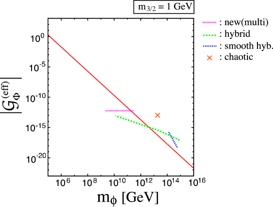
Figure 2: Upper bound on the (effective) auxiliary field of the inflaton ${\cal G}^{\rm(eff)}_{\Phi}$ as a function of the inflaton mass $m_{\phi}$, with $m_{3/2}=1{\rm\,GeV}$. We set $m_{\tilde{g}_{3}}=500$ GeV. $T_{R}$ is set to be the largest allowed value, and the bound becomes severer for lower $T_{R}$. The typical values of ${\cal G}^{\rm(eff)}_{\Phi}$ and $m_{\phi}$ for the multi-field new, hybrid, smooth hybrid, and chaotic inflation models with $\kappa=1$ are also shown. The chaotic inflation can avoid this bound by assuming $Z_{2}$ symmetry (see the text for details).

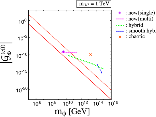
Figure 3: Same as Fig. 2 except for $m_{3/2}=1{\rm\,TeV}$. The typical values of ${\cal G}^{\rm(eff)}_{\Phi}$ and $m_{\phi}$ for the single-field new inflation model with $\kappa=1$ are also plotted. The solid and dashed lines are for the hadronic branching ratio $B_{h}=1$ and $10^{-3}$, respectively.

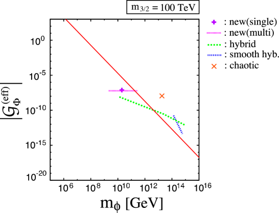
Figure 4: Same as Fig. 3 except for $m_{3/2}=100{\rm\,TeV}$.

5 Explicit calculation of ${\cal G}^{\rm(eff)}_{\Phi}$ for several inflation models

In estimating the effective coupling of the inflaton $\phi$ with the gravitino, the mixings with the SUSY breaking sector field is important, as pointed in Ref. [29] for specific cases. In fact one can rigorously estimate the coupling in a rather generic way [30]. In this section, we would like to show how to obtain ${\cal G}^{\rm(eff)}_{\Phi}$, based on the argument of Ref. [30].

The point is that the inflaton field $\phi$ does not coincide with the mass eigenstate after inflation due to the mixings with the SUSY breaking sector field $z$. There are three sources for the mixings: (i) kinetic terms (or equivalently, the Kähler metric); (ii) non-analytic (NA) mass terms; (iii) analytic (A) mass terms. Although the mixing in the Kähler metric can be important for the reheating processes [30], we neglect it here since it does not affect the coupling with the gravitinos. In the following we focus on the mixings in the mass terms.

5.1 Single-field inflation model

Let us first consider a single-field inflation model, with the Käler metric $g_{ij^{*}}=\delta_{ij}$. In the Einstein frame, the SUGRA Lagrangian contains the scalar potential, $V=e^{G}(G^{i}G_{i}-3)$. The non-analytic (NA) and analytic (A) mass terms are written as

$$M_{ij*}^{2} = \frac{\partial^{2}V}{\partial\varphi^{i}\partial\varphi^{\dagger j}}\;=\;e^{G}\left(\nabla_{i}G_{k}\nabla_{j*}G^{k}-R_{ij^{*}k\ell^{*}}G^{k}G^{\ell*}+g_{ij^{*}}\right),$$ (45)

$$M_{ij}^{2} = M_{ji}^{2}\;=\;\frac{\partial^{2}V}{\partial\varphi^{i}\partial\varphi^{j}}\;=\;e^{G}\left(\nabla_{i}G_{j}+\nabla_{j}G_{i}+G^{k}\nabla_{i}\nabla_{j}G_{k}\right),$$ (46)

respectively, where we have assumed the vanishing cosmological constant, $G^{i}G_{i}=3$, and used the potential minimization condition, $G^{i}\nabla_{k}G_{i}+G_{k}=0$ in the vacuum. The gravitino mass is given by $m_{3/2}=\left\langle e^{G/2}\right\rangle$. Here $R_{ij^{*}k\ell^{*}}$ is the curvature of the Kähler manifold, defined by $R_{ij^{*}k\ell^{*}}=g_{ij^{*}k\ell^{*}}-g^{mn^{*}}g_{mj^{*}\ell^{*}}g_{n^{*}ik}$. Also the covariant derivative of $G_{i}$ is defined by $\nabla_{i}G_{j}=G_{ij}-\Gamma^{k}_{ij}G_{k}$, where the connection, $\Gamma_{ij}^{k}=g^{k\ell^{*}}g_{ij\ell^{*}}$, and $\nabla_{k}g_{ij^{*}}=0$ is satisfied.

We assume that the inflaton $\phi$ is heavy due to a large supersymmetric mass, $m_{\phi}\equiv|e^{G/2}\nabla_{\phi}G_{\phi}|\gg m_{3/2}$, and that $M^{2}_{\phi\bar{\phi}}$ dominates over the other elements of the mass terms. Then the NA mass terms can be diagonalized by the following transformation:

$$\Phi \equiv \phi+\epsilon z,$$

$$Z \equiv z-\epsilon^{*}\phi,$$ (47)

where $\epsilon$ represents the mixing angle. Here we have assumed $|\epsilon|\ll 1$ and neglected those terms of $O(\epsilon^{2})$. Since $M_{\phi\bar{\phi}}^{2}$ dominates over the other components in the mass matrix, the mixing angle is given by the ratio of $M_{\phi\bar{\phi}}^{2}$ to the off-diagonal component:

$$\epsilon\simeq\frac{M_{z\bar{\phi}}^{2}}{M_{\phi\bar{\phi}}^{2}}.$$ (48)

As emphasized in Ref. [30], the NA mass eigenstates $(\Phi,Z)$ do not necessarily coincide with the true mass eigenstates. In fact, the analytic mass terms generically provide further mixing between $\phi$ and $z^{\dagger}$. The true mass eigenstates are therefore

$$\tilde{\Phi} \equiv \phi+\epsilon z+\tilde{\epsilon}z^{\dagger},$$ (49)

$$\tilde{Z} \equiv z-\epsilon^{*}\phi-\tilde{\epsilon}\phi^{\dagger},$$ (50)

where the mixing angle $\tilde{\epsilon}$, which is assumed to be much smaller than unity, is given by

$$\tilde{\epsilon}\;\simeq\;\frac{M_{\bar{\phi}\bar{z}}^{2}}{M_{\phi\bar{\phi}}^{2}}.$$ (51)

Below we show that the coupling with the gravitinos is suppressed in the NA mass eigenstates, but it is not the case in the true mass eigenstates if the Kähler potential is non-minimal.

In the NA mass eigenstates, the off-diagonal element of the non-analytic mass term is zero by definition:

$$M^{2}_{\Phi\bar{Z}}=e^{G}\left(\nabla_{\Phi}G_{\Phi}\nabla_{\bar{Z}}G_{\bar{\Phi}}+\nabla_{\Phi}G_{Z}\nabla_{\bar{Z}}G_{\bar{Z}}-R_{\Phi\bar{Z}ij^{*}}G^{i}G^{j^{*}}\right)=0,$$ (52)

which leads to

$$\nabla_{\bar{Z}}G_{\bar{\Phi}}\;\simeq\;\frac{R_{\Phi\bar{Z}ij^{*}}G^{i}G^{j^{*}}}{\nabla_{\Phi}G_{\Phi}},$$ (53)

where we have used $|\nabla_{\Phi}G_{\Phi}|\gg|\nabla_{Z}G_{Z}|$. On the other hand, the potential minimization condition for $\Phi$ reads

$$G_{\bar{\Phi}}\nabla_{\Phi}G_{\Phi}+G_{\bar{Z}}\nabla_{\Phi}G_{Z}+G_{\Phi}=0,$$ (54)

which can be solved for $G_{\Phi}$:

$$G_{\Phi}\;\simeq\;-\frac{\nabla_{\bar{\Phi}}G_{\bar{Z}}}{\nabla_{\bar{\Phi}}G_{\bar{\Phi}}}G_{Z}.$$ (55)

Substituting (53) into (55), we arrive at

$$|G_{\Phi}|\;\simeq\;3\sqrt{3}\frac{|R_{\Phi\bar{Z}Z\bar{Z}}|}{|\nabla_{\bar{\Phi}}G_{\bar{\Phi}}|^{2}},$$ (56)

where we have used $|G_{Z}|=|G^{Z}|\simeq\sqrt{3}$. Thus $G_{\Phi}$ is always proportional to $m_{3/2}^{2}/m_{\phi}^{2}\ll 1$. For the minimal Kähler potential, $G_{\Phi}$ is exactly zero in this basis. In the mass-eigenstate basis, therefore, the effective coupling of the inflaton $\tilde{\Phi}$ with the gravitinos dominantly comes from the mixing in the analytic mass terms:

$$|{\cal G}^{\rm(eff)}_{\Phi}|\;\simeq\;\left|\tilde{\epsilon}\,G_{z}\right|\simeq 3|g_{\bar{\phi}zz}|\frac{m_{3/2}}{m_{\phi}}.$$ (57)

For instance, let us consider $\delta K=(1/2)\kappa|\phi|^{2}zz+{\rm h.c.}$, which is expected to be present if $z$ is singlet under any symmetries. For the non-minimal Kähler potential, the effective coupling becomes

$$|{\cal G}^{\rm(eff)}_{\Phi}|\;\simeq\;3\kappa\left\langle\phi\right\rangle\frac{m_{3/2}}{m_{\phi}},$$ (58)

where $\left\langle\phi\right\rangle$ denotes the vacuum expectation value (VEV) of $\phi$. Therefore, ${\cal G}^{\rm(eff)}_{\Phi}$ is proportional to $G_{\phi}\sim\left\langle\phi\right\rangle m_{3/2}/m_{\phi}$ [2], for this choice of the interaction between $\phi$ and $z$.

Here let us comment on the case that the mass of the SUSY breaking field $\tilde{Z}$, $m_{z}$, is larger than $m_{\phi}$ due to the non-SUSY mass term. Such situation may be realized in the dynamical SUSY breaking models [24]. Then the $|{\cal G}^{\rm(eff)}_{\Phi}|$ becomes of $O(\left\langle\phi\right\rangle m_{3/2}/m_{\phi})$ even if the Kähler potential is minimal [29, 30]. To be conservative, however, we assume that $m_{\phi}>m_{z}$ in the following discussion.

As a concrete example, here we study the new inflation model [35, 36, 37]. In the new inflation model, the Kähler potential and superpotential of the inflaton sector are written as

$$K(\phi,\phi^{\dagger}) = |\phi|^{2}+\frac{k}{4}|\phi|^{4},$$

$$W(\phi) = v^{2}\phi-\frac{g}{n+1}\,\phi^{n+1}.$$ (59)

where the observed density fluctuations are explained for $v=4\times 10^{-7}\,(0.1/g)^{1/2}$ and $k\mathop{}_{\textstyle\sim}^{\textstyle<}0.03$ in the case of $n=4$ [37]. After inflation, the inflaton $\phi$ takes the expectation value $\left\langle\phi\right\rangle\simeq(v^{2}/g)^{1/n}$. In this model the inflaton mass is given by $m_{\phi}\simeq nv^{2}/\left\langle\phi\right\rangle$, and the gravitino mass is related to $v$ as $m_{3/2}\simeq nv^{2}\left\langle\phi\right\rangle/(n+1)$, since the inflaton induces the spontaneous breaking of the $R$-symmetry. Thus, (57) leads to 

$$|{\cal G}^{\rm(eff)}_{\Phi}|\simeq\frac{3}{n+1}|g_{\bar{\phi}zz}|\left(\frac{v^{2}}{g}\right)^{\frac{2}{n}}.$$ (60)

For the interaction $\delta K=(1/2)\kappa|\phi|^{2}zz+{\rm h.c.}$, this becomes

$$|{\cal G}^{\rm(eff)}_{\Phi}|\simeq\frac{3\kappa}{n+1}\left(\frac{v^{2}}{g}\right)^{\frac{3}{n}}.$$ (61)

In the case of $n=4$, $|{\cal G}^{\rm(eff)}_{\Phi}|\simeq 8\times 10^{-10}\kappa$ and $m_{\phi}\simeq 4\times 10^{9}$ GeV for $m_{3/2}=1$ TeV, while $|{\cal G}^{\rm(eff)}_{\Phi}|\simeq 8\times 10^{-8}\kappa$ and $m_{\phi}\simeq 2\times 10^{10}$ GeV for $m_{3/2}=100$ TeV. Note that $m_{3/2}\ll 1\,$TeV cannot be realized unless $g\gg 1$. We plot these results with $\kappa=1$ in Figs. 3 and 4. We can see that the new inflation model is on the verge of being excluded for $m_{3/2}=1$ TeV , while it is close to but slightly below the bound for $m_{3/2}=100$ TeV. This single-field new inflation model will be discussed in detail in Ref. [39].

5.2 Multiple-field inflation model

Next we consider an inflation model with multiple fields, for which the formula (57) cannot be simply applied as it is. Although we generically need to evaluate ${\cal G}^{\rm(eff)}_{\Phi}$ for each inflation model, there is an important class of models described by the following superpotential:

$$W(\phi,\psi)\;=\;\phi f(\psi),$$ (62)

where $f(\psi)$ is a function of $\psi$. The potential minimum in the global SUSY limit is located at

$$\left\langle\phi\right\rangle = 0,$$

$$\left\langle\psi\right\rangle = \psi_{0},$$ (63)

where $\psi_{0}$ satisfies $f(\psi_{0})=0$. Note that the true minimum is slightly displaced from (63), once the SUSY breaking field is taken into account [2, 40].

For instance, the above class of the models includes a new inflation model [41] and a hybrid inflation model [42, 43, 44], described by

$$W(\phi,\psi)\;=\;\phi\left(\mu^{2}-\frac{\psi^{n}}{M^{n-2}}\right),$$ (64)

where $\mu$ determines the inflation energy scale and $M$ is an effective cut-off scale. In the new inflation model $\psi$ plays a role of the inflaton, while $\phi$ is the inflaton in the hybrid inflation model.

The inflaton fields $\phi$ and $\psi$ have almost the same masses,

$$m_{\phi}\;\simeq\;m_{\psi}\;\simeq\;\left|e^{G/2}\nabla_{\phi}G_{\psi}\right|,$$ (65)

which are assumed to be much larger than the gravitino mass. It should be noted that $\phi$ and $\psi$ (and/or $\psi^{\dagger}$) almost maximally mix with each other to form the mass eigenstates due to the almost degenerate masses. To see this let us take the NA mass-eigenstate basis $(\Phi,\Psi,Z)$ in which the non-analytic mass matrix is diagonalized except for $\phi-\psi$ mixing. The difference between the diagonal components of the non-analytic mass matrix is small: $|M^{2}_{\Phi\bar{\Phi}}-M^{2}_{\Psi\bar{\Psi}}|=O(m_{3/2}^{2})$, while the off-diagonal component in the analytic mass matrix is relatively large: $M^{2}_{\Phi\Psi}=O(m_{3/2}m_{\phi})$ , resulting in the almost maximal mixing between $\phi$ and $\psi^{\dagger}$. This mixing is effective at the inflaton decay, since the Hubble parameter at the decay should be (much) smaller than $O(m_{3/2})$ to satisfy the bounds from the thermally produced gravitinos. However, since the mixing is due to the specific character of (62) and it occurs within the inflaton sector, we leave it for a moment. Then we can similarly show that the auxiliary fields $G_{\Phi}$ and $G_{\Psi}$ are proportional to $m_{3/2}^{2}/m_{\phi}^{2}$ in the NA mass eigenstates $(\Phi,\Psi,Z)$. Therefore the effective couplings with the gravitinos arise mainly from the mixings in the analytic mass terms, as in the single-field inflation :

$$|{\cal G}^{\rm(eff)}_{\Phi}| \simeq 3|g_{\bar{\psi}zz}|\frac{m_{3/2}}{m_{\phi}},$$

$$|{\cal G}^{\rm(eff)}_{\Psi}| \simeq 3|g_{\bar{\phi}zz}|\frac{m_{3/2}}{m_{\psi}}.$$ (66)

For such interactions as $\delta K=(\kappa/2)|\psi|^{2}zz+(\tilde{\kappa}/2)|\phi|^{2}zz+{\rm h.c.}$, we have

$$|{\cal G}^{\rm(eff)}_{\Phi}| \simeq 3\kappa\left\langle\psi\right\rangle\frac{m_{3/2}}{m_{\phi}},$$

$$|{\cal G}^{\rm(eff)}_{\Psi}| \simeq 3\tilde{\kappa}\left\langle\phi\right\rangle\frac{m_{3/2}}{m_{\psi}}.$$ (67)

Therefore $|{\cal G}^{\rm(eff)}_{\Psi}|$ is suppressed compared to $|{\cal G}^{\rm(eff)}_{\Phi}|$ if $\left\langle\psi\right\rangle\gg\left\langle\phi\right\rangle$ as in the case of (64).

The true mass eigenstates are obtained after taking account of the (almost) maximal mixing between $\phi$ and $\psi(\psi^{\dagger})$ discussed above:

$$\varphi_{\pm}\;\simeq\frac{\phi\pm\psi^{({\dagger})}}{\sqrt{2}},$$ (68)

where we have omitted the relatively small mixings with $z$ for simplicity, but they are included in the definition of $\varphi_{\pm}$. For $|{\cal G}^{\rm(eff)}_{\Phi}|\gg|{\cal G}^{\rm(eff)}_{\Psi}|$, the effective couplings of $\varphi_{\pm}$ with the gravitinos are roughly given by

$$|{\cal G}^{\rm(eff)}_{\varphi_{\pm}}|\;\simeq\;\frac{1}{\sqrt{2}}|{\cal G}^{\rm(eff)}_{\Phi}|.$$ (69)

5.2.1 New inflation model

The new inflation discussed in Sec. 5.1 is also realized for [41]

$$K = |\phi|^{2}+|\psi|^{2}+\frac{k_{1}}{4}|\phi|^{4}+k_{2}|\phi|^{2}|\psi|^{2}+\frac{k_{3}}{4}|\psi|^{4},$$

$$W = \phi(v^{2}-g\,\psi^{4}),$$ (70)

in which the inflaton is $\psi$, while $\phi$ stays at the origin during and after inflation . If one defines $k\equiv k_{2}-1$, the scalar potential for the inflaton $\psi$ becomes the same as the single-field new inflation model, although the gravitino mass is not related to the inflaton parameters. After the inflation ends, the energy of the universe is dominated by the oscillation energy of $\psi$ . Although ${\cal G}^{\rm(eff)}_{\Psi}$ is suppressed compared to ${\cal G}^{\rm(eff)}_{\Phi}$, the effective coupling to the gravitinos is given by (69), since $\phi$ and $\psi$ almost maximally mixes with each other in the vacuum. Thus the constraint on this model is comparable to that on the single-field new inflation. For the non-minimal coupling $\delta K=(1/2)\kappa|\psi|^{2}zz+{\rm h.c.}$, the effective coupling to the gravitinos is given by

$$|{\cal G}^{\rm(eff)}_{\varphi_{\pm}}| \simeq \frac{3}{\sqrt{2}}\kappa\left\langle\psi\right\rangle\frac{m_{3/2}}{m_{\phi}}.$$ (71)

We plot the value of $|{\cal G}^{\rm(eff)}_{\varphi_{\pm}}|$ for $g=10^{-4}-1$ and $k=10^{-4}-10^{-1.5}$ with the e-folding number $N=50$ in Figs. 2, 3, and 4. Thus the (multi-field) new inflation model is on the verge of being excluded, if $\kappa$ is order unity.

5.2.2 Hybrid inflation model

The hybrid inflation model contains two kinds of superfields: one is $\phi$ which plays a role of inflaton and the others are waterfall fields $\psi$ and $\tilde{\psi}$ [42, 43, 44]. After inflation ends, $\phi$ as well as $\psi$($\tilde{\psi}$) oscillates around the potential minimum and dominates the universe until the reheating.

The superpotential $W(\phi,\psi,\tilde{\psi})$ for the inflaton sector is

$$W(\phi,\psi,\tilde{\psi})=\phi(\mu^{2}-\lambda\tilde{\psi}\psi),$$ (72)

where $\psi$ and $\tilde{\psi}$ are assumed to be charged under $U(1)$ gauge symmetry. Here $\lambda$ is a coupling constant and $\mu$ is the inflation energy scale. The potential minimum is located at $\left\langle\phi\right\rangle=0$ and $\langle\psi\rangle=\langle\tilde{\psi}\rangle=\mu/\sqrt{\lambda}$ in the SUSY limit. For a successful inflation, $\mu$ and $\lambda$ are related as $\mu\simeq 2\times 10^{-3}\lambda^{1/2}$ for $\lambda\mathop{}_{\textstyle\sim}^{\textstyle>}10^{-3}$, and $\mu\simeq 2\times 10^{-2}\lambda^{5/6}$ for $\lambda\mathop{}_{\textstyle\sim}^{\textstyle<}10^{-3}$. Moreover, in this type of hybrid inflation there exists a problem of cosmic string formation because $\psi$ and $\tilde{\psi}$ have $U(1)$ gauge charges. To avoid the problem the coupling $\lambda$ should be small as, $\lambda\sim 10^{-4}$ [47].

Due to the D-term potential one linear combination of $\psi$ and $\tilde{\psi}$, given by $\psi^{(-)}\equiv(\psi-\tilde{\psi})/\sqrt{2}$, has a large mass of $\sim g\left\langle\psi\right\rangle$ ($g$ denotes the gauge coupling), while the other, $\psi^{(+)}\equiv(\psi+\tilde{\psi})/\sqrt{2}$ has a mass equal to that of $\phi$: $m_{\psi^{(+)}}=m_{\phi}=\sqrt{2}\lambda\langle\psi\rangle$. It is the latter that (almost) maximally mixes with $\phi$ to form mass eigenstates. Since the form of the superpotential is almost identical to (64), it is straightforward to extend the results (66) and (69) to obtain

$$|{\cal G}^{\rm(eff)}_{\varphi_{\pm}}| \simeq \frac{3}{\sqrt{2}}\kappa(\sqrt{2}\langle\psi\rangle)\frac{m_{3/2}}{m_{\phi}},$$ (73)

for the non-minimal coupling $\delta K=(1/2)\kappa|\psi^{(+)}|^{2}zz+{\rm h.c.}$. Note that VEV of $\psi^{(+)}$ is equal to $\sqrt{2}\langle\psi\rangle$.

For $\lambda\sim 10^{-1}-10^{-5}$ [48] we obtain $\mu\sim 8\times 10^{-4}-1\times 10^{-6}$, $|{\cal G}^{\rm(eff)}_{\varphi_{\pm}}|\sim 9\times 10^{-15}\kappa(m_{3/2}/1{\rm\,TeV})-9\times 10^{-11}\kappa(m_{3/2}/1{\rm\,TeV})$ and $m_{\phi}\sim 8\times 10^{14}-1\times 10^{10}$ GeV. From Fig. 3, one can see the hybrid inflation model is almost excluded by the gravitino overproduction for $m_{3/2}=1{\rm\,TeV}$, if $\kappa$ is order unity. For $m_{3/2}=1{\rm\,GeV}$ and $100\,$TeV, the constraints become slightly mild, but a significant fraction of the parameter space is still excluded (see Figs. 2 and 4). Although the constraints on $|{\cal G}^{\rm(eff)}_{\varphi_{\pm}}|$ become relaxed for smaller $m_{\phi}$ (i.e., smaller $\lambda\mathop{}_{\textstyle\sim}^{\textstyle<}10^{-4}$), it is then somewhat disfavored by the WMAP data [20] since the density fluctuation becomes almost scale-invariant.

Next let us consider a smooth hybrid inflation model [49], which predicts the scalar spectral index as $n_{s}\simeq 0.97$, which is slightly smaller than the simple hybrid inflation model. The superpotential of the inflaton sector is

$$W(\phi,\psi,\tilde{\psi})=\phi\left(\mu^{2}-\frac{(\tilde{\psi}\psi)^{n}}{M^{2n-2}}\right).$$ (74)

The VEVs of $\psi$ and $\tilde{\psi}$ are given by $\left\langle\psi\right\rangle=\left\langle\tilde{\psi}\right\rangle=(\mu M^{n-1})^{1/n}$, and we assume that $\psi=\tilde{\psi}$ always holds due to the additional D-term potential. Then one of the combination, $\psi^{(+)}\equiv(\psi+\tilde{\psi})/\sqrt{2}$, mixes with $\phi$, and the effective coupling with the gravitinos is given by

$$|{\cal G}^{\rm(eff)}_{\varphi_{\pm}}| \simeq \frac{3}{\sqrt{2}}\kappa(\sqrt{2}\langle\psi\rangle)\frac{m_{3/2}}{m_{\phi}},$$ (75)

for $\delta K=(1/2)\kappa|\psi^{(+)}|^{2}zz+{\rm h.c.}$. Here we have defined $m_{\phi}=\sqrt{2}n\mu^{2}/\left\langle\psi\right\rangle$. The constraint on the model is more or less similar to that on the hybrid inflation model. In fact, for $n=2$ we obtain $\mu\sim 4\times 10^{-4}-9\times 10^{-5}$, $|{\cal G}^{\rm(eff)}_{\varphi_{\pm}}|\sim 2\times 10^{-13}\kappa(m_{3/2}/1{\rm\,TeV})-4\times 10^{-16}\kappa(m_{3/2}/1{\rm\,TeV})$ and $m_{\phi}\sim 1\times 10^{14}-6\times 10^{14}$ GeV. From Figs. 2 - 4 one can see that the smooth hybrid inflation model is excluded for a broad range of $m_{3/2}$ for $\kappa=O(1)$.

Lastly let us comment on the D-term inflation model [50], in which one of the waterfall fields, $\psi_{-}$, obtains a large VEV of $\sim 10^{16}{\rm\,GeV}$. The $\psi_{-}$ field can decay into a pair of the gravitino if there is a coupling like $|\psi_{-}|^{2}zz/2+{\rm h.c.}$ in the Kähler potential. However, after inflation, the universe is dominated by the two fields: one is the $\psi_{-}$ field and the other is the inflaton, $S$. The resultant gravitino abundance thus depends on both the reheating processes of these two fields and the relative portion of the energy in each field [51]. Therefore we cannot put a rigorous bound on the D-term inflation model.

5.2.3 Chaotic inflation model

A chaotic inflation [52] is realized in SUGRA, based on a Nambu-Goldstone-like shift symmetry of the inflaton chiral multiplet $\phi$  [53, 54]. Namely, we assume that the Kähler potential $K(\phi,\phi^{\dagger})$ is invariant under the shift of $\phi$,

$$\phi\rightarrow\phi+i\,A,$$ (76)

where $A$ is a dimensionless real parameter. Thus, the Kähler potential is a function of $\phi+\phi^{\dagger}$; $K(\phi,\phi^{\dagger})=K(\phi+\phi^{\dagger})=c\,(\phi+\phi^{\dagger})+\frac{1}{2}(\phi+\phi^{\dagger})^{2}+\cdots$, where $c$ is a real constant and must be smaller than $O(1)$ for a successful inflation. We will identify its imaginary part with the inflaton field $\varphi\equiv\sqrt{2}{\rm\,Im}[\phi]$. Moreover, we introduce a small breaking term of the shift symmetry in the superpotential in order for the inflaton $\varphi$ to have a potential:

$$W(\phi,\psi)=m\,\phi\,\psi,$$ (77)

where we introduced a new chiral multiplet $\psi$, and $m\simeq 10^{13}$GeV determines the inflaton mass.

The scalar potential is given by

$$V(\eta,\varphi,\psi) = m^{2}e^{K}\left[|\psi|^{2}\left(1+2\left(\eta+\frac{c}{\sqrt{2}}\right)\eta+\left(\eta+\frac{c}{\sqrt{2}}\right)^{2}(\eta^{2}+\varphi^{2})\right)\right.$$ (78)

$$\left.~{}~{}~{}~{}~{}~{}~{}~{}~{}+\frac{1}{2}(\eta^{2}+\varphi^{2})(1-|\psi|^{2}+|\psi|^{4})\right]$$

with

$$K\;=\;\left(\eta+\frac{c}{\sqrt{2}}\right)^{2}-\frac{c^{2}}{2}+|\psi|^{2},$$ (79)

where we have assumed the minimal Kähler potential for $\psi$, and defined $\eta\equiv\sqrt{2}{\rm\,Re}[\phi]$. Note that $\eta$ and $\psi$ cannot be larger than the Planck scale, due to the prefactor $e^{K}$. On the other hand, $\varphi$ can be larger than the Planck scale  [53], since $\varphi$ does not appear in $K$. For $\varphi\gg 1$, $\eta$ acquires the mass comparable to the Hubble parameter and quickly settles down to the minimum, $\eta\simeq-c/\sqrt{2}$. Then the scalar potential during inflation is given by

$$V(\eta,\varphi,\psi)\;\simeq\;\frac{1}{2}m^{2}\varphi^{2}+m^{2}|\psi|^{2}.$$ (80)

For $\varphi\gg 1$ and $|\psi|<1$, the $\varphi$ field dominates the potential and the chaotic inflation takes place (for details see Refs [53, 54]).

The effective auxiliary field of $\psi$ is given by

$$|{\cal G}^{\rm(eff)}_{\Psi}|\simeq 3g_{\bar{\phi}zz}\frac{m_{3/2}}{m}=3\kappa\frac{m_{3/2}}{m},$$ (81)

where we have assumed the non-minimal coupling $\delta K=(1/2)\kappa(\phi+\phi^{\dagger})zz+{\rm h.c.}$ in the second equality. This Kähler potential is invariant under the shift symmetry (76). Note that $|{\cal G}^{\rm(eff)}_{\Phi}|$ is suppressed for e.g., $\delta K=(1/2)\tilde{\kappa}|\psi|^{2}zz+{\rm h.c.}$ due to $\left\langle\psi\right\rangle\ll 1$. Taking account of the mixing between $\phi$ and $\psi^{\dagger}$, the effective coupling with the gravitinos is given by

$$|{\cal G}^{\rm(eff)}_{\varphi_{\pm}}|\simeq\frac{3}{\sqrt{2}}\kappa\frac{m_{3/2}}{m}.$$ (82)

It is worth noting that both real and imaginary components of $\phi$ can decay into a pair of the gravitinos via the mixings with $z$ and $\psi$. One might suspect that it is only the real component of $\phi$ that can decay into the gravitinos, since the shift symmetry dictates that the only real component $(\phi+\phi^{\dagger})$ appears in the Kähler potential. However, it is not surprising that this is not the case, since the enhanced decay amplitude is proportional to powers of the large SUSY mass $m$ that explicitly violates the shift symmetry.

We plot the result (82) with $\kappa=1$ in Figs. 2, 3, and 4. Although the coupling is too large if $\kappa=O(1)$, it should be noted that in this chaotic inflation model we can realize $|{\cal G}^{\rm(eff)}_{\varphi_{\pm}}|\simeq 0$ by assuming an approximate $Z_{2}$ symmetry. Therefore, the new gravitino problem does not exist in this case. A detailed discussion on the chaotic inflation model will be given in [55].

6 Conclusions

Throughout this paper we have assumed no entropy production late after the reheating of inflation. We briefly discuss potential problems when a late-time entropy production [56] occurs. First of all, the cosmological constraints on the reheating temperature shown in Sec. 3 would be relaxed and the Hubble parameter at the inflaton-decay time does not necessarily satisfy the condition $H<m_{3/2}$ for the formula (29) to be applicable. Thus, the cosmological constraints on ${\cal G}^{\rm(eff)}_{\Phi}$ would become milder . On the other hand, we must be careful about the gravitino production in decay processes of the field $X$ responsible for the late-time reheating. One may have a similar stringent constraint on ${\cal G}^{\rm(eff)}_{X}$. An obvious way to induce late-time entropy production avoiding the problem is to assume the late-time decay of a scalar field with a mass smaller than $2m_{3/2}$. In addition, there is another interesting example that is free from the problem. Consider that the scalar partner of a right-handed neutrino $N$ possesses a large value during the inflation. If the value is at the Planck scale and its decay rate is small, the scalar $N$ dominates the universe before its decay. Thus, the decay of the scalar $N$ can produce entropy and dilute the abundance of the relic gravitino. The crucial point here is that the scalar $N$ does not decay into a pair of gravitinos due to the matter (or lepton-number) parity conservation. In other word, $N$ does not mix with the SUSY breaking field. Thus, this decay process is free from the gravitino-overproduction problem. Furthermore, the decay of the scalar $N$ may generate the baryon asymmetry of the universe [57] through the leptogenesis [58].

Another even manifest solution to the gravitino overproduction problem is to assume the gravitino mass $m_{3/2}<O(10)\,$eV [22]. In this case, the produced gravitinos get into thermal equilibrium due to relatively strong interactions with the standard-model particles, and such light gravitinos are cosmologically harmless.

Let us comment on another decay mode induced by non-minimal couplings between the inflaton $\phi$ and the SUSY breaking field $z$. From (57) and (66), the gravitino production rate is proportional to $|g_{\bar{\phi}zz}|^{2}$. If $g_{\bar{\phi}zz}$ is nonzero, the inflaton $\phi$ can also decay into the SUSY breaking field $z$ [30], and the partial decay rate is comparable to that into the gravitinos. As noted in Ref. [30], thus produced $z$ may cause a cosmological problem at most as severe as that induced by the gravitinos. Therefore including the effect of the $z$ production may make the problem only a few times worse, and our discussion remains qualitatively unchanged.

In this paper we have shown that an inflation model generically leads to the gravitino overproduction, which can jeopardize the successful standard cosmology. We have explicitly calculated the effective auxiliary field ${\cal G}^{\rm(eff)}_{\Phi}$, which is an important parameter to determine the gravitino abundance, for several inflation models. The new inflation is on the verge of being excluded, while the (smooth) hybrid inflation model is excluded if $\kappa=O(1)$. To put it differently, the coefficient of the non-minimal coupling in the Kähler potential, $\kappa$, must be suppressed especially in (smooth) the hybrid inflation model. We show the constraints on $\kappa$ for the inflation model we studied so far in Figs. 5 - 7. As long as the SUSY breaking field $z$ is singlet, there is no reason that $\kappa$ should be suppressed. Therefore those inflation models required to have $\kappa\ll 1$ involve severe fine-tunings on the non-renormalizable interactions with the SUSY breaking field, which makes either the inflation models or the SUSY breaking models containing the singlet $z$ (with $G_{z}=O(1)$) strongly disfavored. We stress again that the existence of such a singlet field is required in the gravity-mediated SUSY breaking, in order to give the SM gauginos a mass comparable to the squark and slepton masses. One of the most attractive ways to get around this new gravitino problem is to postulate a symmetry of the inflaton, which is preserved at the vacuum, to forbid the mixing with the SUSY breaking field. Among the known models, such a chaotic inflation model can avoid the potential gravitino overproduction problem by assuming $Z_{2}$ symmetry. Another is to assign some symmetry on the SUSY breaking field $z$ as in the gauge-mediated [7] and anomaly-mediated [3] SUSY breaking models. So far we have assumed that $z$ is singlet under any symmetries as in the gravity-mediated SUSY breaking models. If the SUSY breaking field $z$ is not a singlet, and the non-minimal coupling like $\delta K=\kappa/2|\phi|^{2}zz+{\rm h.c.}$ can be suppressed. It should be noted however that the mixing between $\phi$ and $z$ may induce other cosmological problems [30] even if $z$ is charged under some symmetry and/or its VEV is suppressed.

Although we have briefly discussed various (typical) inflation models, it should be stressed that the gravitino-overproduction problem is common to all the inflation models in SUGRA. Thus, in inflation model building, one must always check whether an inflation model under consideration satisfies the bound.

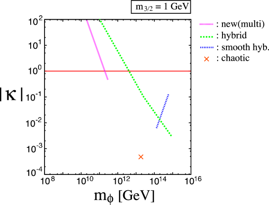
Figure 5: Upperbounds on $\kappa$ as a function of the inflaton mass $m_{\phi}$, with $m_{3/2}=1{\rm\,GeV}$, for the multi-field new, hybrid, and smooth hybrid, and chaotic inflation models are also shown. See the text for the definition of $\kappa$ in each model.

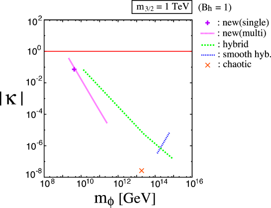
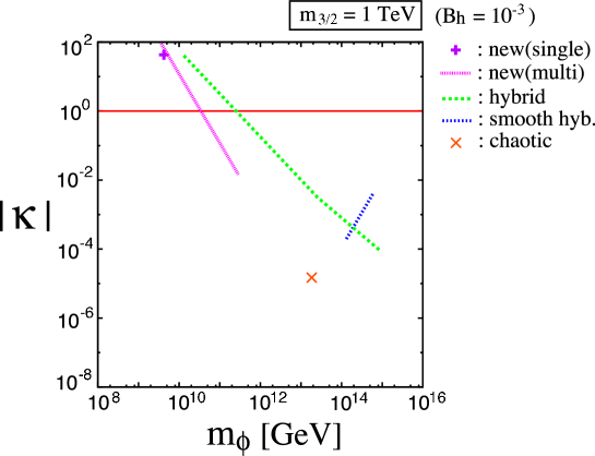
Figure 6: Same as Fig. 5 except for $m_{3/2}=1{\rm\,TeV}$. The bound on the single-field new inflation model is also plotted.

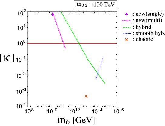
Figure 7: Same as Fig. 6 except for $m_{3/2}=100{\rm\,TeV}$.

References

-
[1]
J. Polchinski, “String Theory”, Volumes 1 and 2, Cambridge university Press, 2000;
M. Green, J. Schwarz, E. Witten, “Superstring Theory”, Volumes 1 and 2, Cambridge University Press, 1987. - [2] M. Kawasaki, F. Takahashi and T. T. Yanagida, arXiv:hep-ph/0603265.
-
[3]
L. Randall and R. Sundrum,
Nucl. Phys. B 557, 79 (1999);
G. F. Giudice, M. A. Luty, H. Murayama and R. Rattazzi, JHEP 9812, 027 (1998);
J. A. Bagger, T. Moroi and E. Poppitz, JHEP 0004, 009 (2000). - [4] J. R. Ellis, K. Enqvist and D. V. Nanopoulos, Phys. Lett. B 147, 99 (1984).
- [5] J. R. Ellis, C. Kounnas and D. V. Nanopoulos, Phys. Lett. B 143, 410 (1984).
- [6] S. Weinberg, Phys. Rev. Lett. 48, 1303 (1982).
- [7] M. Dine, A. E. Nelson and Y. Shirman, Phys. Rev. D 51 (1995) 1362; M. Dine, A. E. Nelson, Y. Nir and Y. Shirman, Phys. Rev. D 53 (1996) 2658; For a review, see, for example, G. F. Giudice and R. Rattazzi, Phys. Rep. 322 (1999) 419, and references therein.
- [8] L. M. Krauss, Nucl. Phys. B 227, 556 (1983).
- [9] D. Lindley, Astrophys. J. 294 (1985) 1; M. Y. Khlopov and A. D. Linde, Phys. Lett. B 138, 265 (1984); F.Balestra et al., Sov. J. Nucl. Phys. 39, 626 (1984); M. Yu. Khlopov, Yu. L. Levitan, E. V. Sedelnikov and I. M. Sobol, Phys. Atom. Nucl. 57 1393 (1994); J. R. Ellis, J. E. Kim and D. V. Nanopoulos, Phys. Lett. B 145, 181 (1984). R. Juszkiewicz, J. Silk and A. Stebbins, Phys. Lett. B 158, 463 (1985); J. R. Ellis, D. V. Nanopoulos and S. Sarkar, Nucl. Phys. B 259 (1985) 175; J. Audouze, D. Lindley and J. Silk, Astrophys. J. 293, L53 (1985); D. Lindley, Phys. Lett. B 171 (1986) 235; M. Kawasaki and K. Sato, Phys. Lett. B 189, 23 (1987); R. J. Scherrer and M. S. Turner, Astrophys. J. 331 (1988) 19; J. R. Ellis et al., Nucl. Phys. B 373, 399 (1992).
- [10] M. Kawasaki and T. Moroi, Prog. Theor. Phys. 93, 879 (1995),
- [11] R. J. Protheroe, T. Stanev and V. S. Berezinsky, Phys. Rev. D 51, 4134 (1995).
- [12] E. Holtmann, M. Kawasaki, K. Kohri and T. Moroi, Phys. Rev. D 60, 023506 (1999).
- [13] K. Jedamzik, Phys. Rev. Lett. 84, 3248 (2000).
- [14] M. Kawasaki, K. Kohri and T. Moroi, Phys. Rev. D 63, 103502 (2001).
- [15] K. Kohri, Phys. Rev. D 64 (2001) 043515.
- [16] R. H. Cyburt, J. R. Ellis, B. D. Fields and K. A. Olive, Phys. Rev. D 67, 103521 (2003).
- [17] T. Moroi, H. Murayama and M. Yamaguchi, Phys. Lett. B 303, 289 (1993).
- [18] M. Bolz, A. Brandenburg and W. Buchmuller, Nucl. Phys. B 606, 518 (2001).
- [19] M. Kawasaki, K. Kohri and T. Moroi, Phys. Lett. B 625, 7 (2005); Phys. Rev. D 71, 083502 (2005).
- [20] D. N. Spergel et al., arXiv:astro-ph/0603449.
- [21] M. Ibe, R. Kitano and H. Murayama, Phys. Rev. D 71, 075003 (2005).
- [22] M. Viel, J. Lesgourgues, M. G. Haehnelt, S. Matarrese and A. Riotto, Phys. Rev. D 71, 063534 (2005).
- [23] J. Wess and J. Bagger, Supersymmetry and Supergravity, (Princeton Unversity Press, 1992).
- [24] E. Witten, Nucl. Phys. B 188, 513 (1981).
-
[25]
T. Banks, D. B. Kaplan and A. E. Nelson,
Phys. Rev. D 49, 779 (1994);
K. I. Izawa and T. Yanagida, Prog. Theor. Phys. 94, 1105 (1995);
A. E. Nelson, Phys. Lett. B 369, 277 (1996). - [26] M. Dine and D. MacIntire, Phys. Rev. D 46, 2594 (1992).
-
[27]
M. Endo, K. Hamaguchi and F. Takahashi,
arXiv:hep-ph/0602061;
S. Nakamura and M. Yamaguchi, arXiv:hep-ph/0602081. - [28] T. Asaka, S. Nakamura and M. Yamaguchi, arXiv:hep-ph/0604132.
- [29] M. Dine, R. Kitano, A. Morisse and Y. Shirman, arXiv:hep-ph/0604140.
- [30] M. Endo, K. Hamaguchi and F. Takahashi, arXiv:hep-ph/0605091.
- [31] R. Casalbuoni, S. De Curtis, D. Dominici, F. Feruglio and R. Gatto, Phys. Lett. B 215, 313 (1988); Phys. Rev. D 39, 2281 (1989).
-
[32]
R. Kallosh, L. Kofman, A. D. Linde and A. Van Proeyen,
Phys. Rev. D 61, 103503 (2000);
G. F. Giudice, I. Tkachev and A. Riotto, JHEP 9908, 009 (1999);
G. F. Giudice, A. Riotto and I. Tkachev, JHEP 9911, 036 (1999);
R. Kallosh, L. Kofman, A. D. Linde and A. Van Proeyen, Class. Quant. Grav. 17, 4269 (2000) [Erratum-ibid. 21, 5017 (2004)]. - [33] H. P. Nilles, M. Peloso and L. Sorbo, Phys. Rev. Lett. 87, 051302 (2001); JHEP 0104, 004 (2001).
- [34] R. Allahverdi, M. Bastero-Gil and A. Mazumdar, Phys. Rev. D 64, 023516 (2001).
- [35] K. Kumekawa, T. Moroi and T. Yanagida, Prog. Theor. Phys. 92, 437 (1994).
- [36] K. I. Izawa and T. Yanagida, Phys. Lett. B 393, 331 (1997).
- [37] M. Ibe, K. I. Izawa, Y. Shinbara and T. T. Yanagida, arXiv:hep-ph/0602192.
- [38] M. Ibe, K. I. Izawa and T. Yanagida, Phys. Rev. D 71, 035005 (2005).
- [39] M. Ibe and Y. Shinbara, in private communication.
- [40] G. R. Dvali, G. Lazarides and Q. Shafi, Phys. Lett. B 424, 259 (1998).
-
[41]
T. Asaka, K. Hamaguchi, M. Kawasaki and T. Yanagida,
Phys. Rev. D 61, 083512 (2000);
V. N. Senoguz and Q. Shafi, Phys. Lett. B 596, 8 (2004). - [42] E. J. Copeland, A. R. Liddle, D. H. Lyth, E. D. Stewart and D. Wands, Phys. Rev. D 49, 6410 (1994).
- [43] G. R. Dvali, Q. Shafi and R. K. Schaefer, Phys. Rev. Lett. 73, 1886 (1994).
- [44] A. D. Linde and A. Riotto, Phys. Rev. D 56, 1841 (1997).
-
[45]
G. N. Felder, J. Garcia-Bellido, P. B. Greene, L. Kofman, A. D. Linde and I. Tkachev,
Phys. Rev. Lett. 87, 011601 (2001);
G. N. Felder, L. Kofman and A. D. Linde, Phys. Rev. D 64, 123517 (2001). - [46] M. Desroche, G. N. Felder, J. M. Kratochvil and A. Linde, Phys. Rev. D 71, 103516 (2005).
- [47] M. Endo, M. Kawasaki and T. Moroi, Phys. Lett. B 569, 73 (2003).
- [48] M. Bastero-Gil, S. F. King and Q. Shafi, arXiv:hep-ph/0604198.
- [49] G. Lazarides and C. Panagiotakopoulos, Phys. Rev. D 52, 559 (1995).
-
[50]
P. Binetruy and G. R. Dvali,
Phys. Lett. B 388, 241 (1996);
E. Halyo, Phys. Lett. B 387, 43 (1996). - [51] C. F. Kolda and J. March-Russell, Phys. Rev. D 60, 023504 (1999)
- [52] A. D. Linde, Phys. Lett. B 129, 177 (1983).
- [53] M. Kawasaki, M. Yamaguchi and T. Yanagida, Phys. Rev. Lett. 85, 3572 (2000).
- [54] M. Kawasaki, M. Yamaguchi and T. Yanagida, Phys. Rev. D 63, 103514 (2001).
- [55] M. Endo, M. Kawasaki, F. Takahashi and T. T. Yanagida, in preparation.
-
[56]
D. H. Lyth and E. D. Stewart,
Phys. Rev. D 53, 1784 (1996);
M. Kawasaki and F. Takahashi, Phys. Lett. B 618, 1 (2005);
see also M. Endo and F. Takahashi, arXiv:hep-ph/0606075. - [57] H. Murayama and T. Yanagida, Phys. Lett. B 322, 349 (1994)
-
[58]
M. Fukugita and T. Yanagida,
Phys. Rev. D 42, 1285 (1990);
see, for a review, W. Buchmuller, R. D. Peccei and T. Yanagida, Ann. Rev. Nucl. Part. Sci. 55, 311 (2005).