Abstract

We perform a complete study of flavour and CP conserving electroweak observables in a slight refinement of a recently proposed five–dimensional model on $R^{4}\times S^{1}/{\bf Z}_{2}$, where the Higgs is the internal component of a gauge field and the Lorentz symmetry is broken in the fifth dimension.

Interestingly enough, the relevant corrections to the electroweak observables turn out to be of universal type and essentially depend only on the value of the Higgs mass and on the scale of new physics, in our case the compactification scale $1/R$. The model passes all constraints for $1/R\geq 4.7$ TeV at 90$\%$ C.L., with a moderate fine–tuning in the parameters. The Higgs mass turns out to be always smaller than 200 GeV although higher values would be allowed, due to a large correction to the $T$ parameter. The lightest non-SM states in the model are typically colored fermions with a mass of order $1-2$ TeV.

1 Introduction

The idea of identifying the Higgs field with the internal component of a gauge field in TeV–sized extra dimensions [2], recently named Gauge-Higgs Unification (GHU), has received a revival of interest in the last years. Although not new (see e.g. [3]), only recently it has been realized that this idea could lead to a solution of the Standard Model (SM) instability of the electroweak scale [4].

Five-dimensional (5D) models, with one extra dimension only, are the simplest and phenomenologically more appealing examples. When the extra dimension is a flat $S^{1}/{\bf Z}_{2}$ orbifold, however, the Higgs and top masses and the scale of new physics, typically given by the inverse of the compactification radius $1/R$, are too low in the simplest implementations of the GHU idea [5]. Roughly speaking, the Higgs mass is generally too light because the Higgs effective potential is radiatively induced, giving rise to a too small effective SM-like quartic coupling. The top is too light because the Yukawa couplings, which are effective couplings in these theories, are engineered in such a way that they are always smaller than the electroweak gauge couplings, essentially due to the 5D Lorentz symmetry. Finally, the scale of new physics is too low, because in minimal models there is no way to generate a sizable gap between the electroweak (EW) scale and $1/R$.

It has recently been pointed out that it is possible to get rid of all the above problems by increasing the Yukawa (gauge) couplings of the Higgs field with the fermions, by assuming a Lorentz symmetry breaking in the fifth direction [6] (see also [7] for other interesting possibilities in a warped scenario). In this way, the Yukawa couplings are not constrained anymore to be smaller than the electroweak gauge couplings and we have the possibility to get Yukawa’s of order one, as needed for the top quark. Stronger Yukawa couplings lead also to a larger effective Higgs quartic coupling, resulting in Higgs masses above the current experimental bound of $m_{H}>115$ GeV. Furthermore, again due to the larger Yukawa couplings, the Higgs effective potential is totally dominated by the fermion contribution. The latter effect, together with a proper choice of the spectrum of (periodic and antiperiodic) 5D fermion fields, can lead to a substantial gap between the EW and compactification scales. In non–universal models of extra dimensions of this sort, where the SM fermions have sizable tree–level couplings with Kaluza–Klein (KK) gauge fields, the electroweak precision tests (EWPT) generically imply quite severe bounds on the compactification scale. At the price of some fine-tuning on the microscopic parameters of the theory, however, one can push $1/R$ in the multi-TeV regime, hoping to get in this way a potentially realistic model.

The SM fermions turn out to be almost localized fields, with the exception of the bottom quark, which shows a partial delocalization, and of the top quark, which is essentially delocalized. This effect generally leads to sizable deviations of the $Z\overline{b}_{L}b_{L}$ coupling with respect to the SM one. Another distortion is introduced in the gauge sector, in order to get the correct weak mixing angle (see [8] for a recent discussion on the difficulty of automatically getting the correct weak-mixing angle in 5D GHU models). The main worrisome effect of the distortion is the departure [6] of the SM $\rho$ parameter from one at tree-level.

Aim of this paper is to consider a variant of the model constructed in [6] and to compute the flavour conserving phenomenological bounds. The main new ingredient is an exact discrete ${\bf Z}_{2}$ symmetry, that we call “mirror symmetry”. It essentially consists in doubling a subset of bulk fields $\phi$, namely all the fermions and some of the gauge fields, in pairs $\phi_{1}$ and $\phi_{2}$ and requiring a symmetry under the interchange $\phi_{1}\leftrightarrow\phi_{2}$. Periodic and antiperiodic fields arise as suitable linear combinations of $\phi_{1}$ and $\phi_{2}$ and the symmetry constrains the couplings of the Higgs with periodic and antiperiodic fermions with the same quantum numbers to be equal. When this is not the case, as in [6], the contributions to the Higgs mass–term of periodic and antiperiodic fields must be finely canceled in order to get a hierarchy between the compactification and EW scale. This adjustment was shown in [6] to be the main source of fine–tuning. Thanks to the mirror symmetry, on the contrary, a natural partial cancellation occurs in the potential. We will see that a difference of an order of magnitude between the compactification and EW scale, with $1/R\sim 1$ TeV, is completely natural in our model. Such a scale is still too low to pass EWPT, but we significantly lower the required amount of fine–tuning. Using the standard definition of [9], thanks to the mirror symmetry, we get a fine-tuning of $O(1\%)$, an order of magnitude better than the $O(1\kern-0.50003pt\raise 2.15277pt\hbox{\sevenrm0}\kern-1.49994pt/\kern-1.49994pt\lower 1.07639pt\hbox{\sevenrm00})$ found in [6]. If quantified with a more refined definition [10] which takes into account the presence of a possible generic sensitivity in the model, but under some physically motivated assumptions, the fine-tuning turns out to be less, of about $O(10\%)$. Another important difference with respect to the model of [6] is the choice of the bulk fermion representations under the electroweak gauge group, which leads to a drastic reduction of the deviation to the SM $Z\overline{b}_{L}b_{L}$ coupling. This reduction is so effective, that the $Z\overline{b}_{L}b_{L}$ distortion becomes negligible in our set-up.

Interestingly enough, all SM states are even under the mirror symmetry, so that the lightest odd particle is absolutely stable. In a large fraction of the parameter space of the model, such a state is the first KK mode of an antiperiodic gauge field. The mirror symmetry represents then an interesting way to get stable non–SM particles in non–universal extra dimensional theories, where KK parity is not a suitable symmetry. Along the lines of [11], it could be interesting to investigate whether such state represents a viable Dark Matter (DM) candidate.

Even assuming flavour and CP conserving new physics effects only, it is necessary to add $18$ dimension $6$ operators to the SM in order to fit the current data (see e.g. [12, 13]). Among such 18 operators, it has recently pointed out that only 10 are sensibly constrained [14]. They can be parametrized by the seven universal parameters $\widehat{S}$, $\widehat{T}$, $\widehat{U}$, $V$, $X$, $W$ and $Y$ introduced in [15], the $\epsilon_{b}$ parameter [16], and other two parameters which describe the deviation of the up and down quark couplings to the $Z$ boson. Due to the way in which light SM fermions couple in our model and to the above suppression of the $Z\overline{b}_{L}b_{L}$ deviation, it turns out that only the four parameters $\widehat{S}$, $\widehat{T}$, $W$ and $Y$ are significant, like in a generic universal model as defined in [15]. Out of the several parameters in our theory, $\widehat{S}$, $\widehat{T}$, $W$ and $Y$ depend essentially only on $m_{H}$ and $1/R$. The result of our fit is reported in fig. 3, which represents one of the main results of this paper. We find that $1/R\geq 4$ TeV with a Higgs mass which can reach up to 600 GeV. Such high values of the Higgs mass are permitted because a relatively high value of the $\widehat{T}$ parameter can be compensated by the effects of a heavy Higgs (see [17] for a discussion of a similar effect in the context of Universal Extra Dimensions (UED) [18]). Although allowed, high values of $m_{H}$ are actually never reached in our model, which predicts $100$ GeV $\leq m_{H}\leq 200$ GeV. As can be seen from fig. 3, our model can successfully pass the combined fit of all electroweak precision observables.

The paper is organized as follows. In section 2 we introduce the model, emphasizing the main points in which it differs from that of [6]. In section 3 we show our results for the combined electroweak observables, including a brief discussion on the fine-tuning of the model. In section 4 we draw our conclusions and in the appendices we collect some useful technical details.

2 The Effective Lagrangian

The 5D model we consider is a slight refinement of the one proposed in [6]. The main essential feature is the introduction of a ${\bf Z}_{2}$ mirror symmetry. The gauge group is taken to be $G=SU(3)_{w}\times G_{1}\times G_{2}$, where $G_{i}=U(1)_{i}\times SU(3)_{i,s}$ , $i=1,2$, with the requirement that the Lagrangian is invariant under the ${\bf Z}_{2}$ symmetry $1\leftrightarrow 2$. The periodicity and parities of the fields on the $S^{1}/{\bf Z}_{2}$ space are the same as in [5, 6] for the electroweak $SU(3)_{w}$ sector, whereas for the abelian $U(1)_{i}$ and non-abelian colored $SU(3)_{i,s}$ fields we now have (omitting for simplicity vector and gauge group indices):

$$A_{1}(y\pm 2\pi R)=A_{2}(y)\,,\;\;\;\;\;\;\;A_{1}(-y)=\eta A_{2}(y)\,,$$ (2.1)

where $\eta_{\mu}=1$, $\eta_{5}=-1$, denoting by greek indices the 4D directions. The unbroken gauge group at $y=0$ is $SU(2)\times U(1)\times G_{+}$, whereas at $y=\pi R$ we have $SU(2)\times U(1)\times G_{1}\times G_{2}$, where $G_{+}$ is the diagonal subgroup of $G_{1}$ and $G_{2}$. The ${\bf Z}_{2}$ mirror symmetry also survives the compactification and remains as an exact symmetry of our construction. It is clear from eq. (2.1) that the linear combinations $A_{\pm}=(A_{1}\pm A_{2})/\sqrt{2}$ are respectively periodic and antiperiodic on $S^{1}$. Under the mirror symmetry, $A_{\pm}\rightarrow\pm A_{\pm}$, so we can assign a multiplicative charge +1 to $A_{+}$ and $-1$ to $A_{-}$. The massless 4D fields are the gauge bosons in the adjoint of $SU(2)\times U(1)\subset SU(3)_{w}$, the $U(1)_{+}$ and gluon gauge fields $A_{+}$ and a charged scalar doublet Higgs field, arising from the internal components of the odd $SU(3)_{w}$ $5D$ gauge fields, namely $A_{w}^{4,5,6,7}$. The $SU(3)_{+,s}$ and $SU(2)$ gauge groups are identified respectively with the SM $SU(3)_{QCD}$ and $SU(2)_{L}$ ones, while the hypercharge $U(1)_{Y}$ is the diagonal subgroup of $U(1)$ and $U(1)_{+}$. The extra $U(1)_{X}$ gauge symmetry which survives the orbifold projection is anomalous (see [5, 6]) and its corresponding gauge boson gets a mass of the order of the cut-off scale $\Lambda$ of the model. An Higgs VEV, i.e. a VEV for the extra-dimensional components of the $SU(3)_{w}$ gauge fields, induces the additional breaking to $U(1)_{EM}$. Following [5, 6], we parametrize this VEV as

$$\langle A_{w\,y}\rangle=\frac{2\alpha}{g_{5}R}t^{7}\,,$$ (2.2)

where $g_{5}$ is the $5D$ charge of the $SU(3)_{w}$ group and $t^{a}$ its generators, normalized as $2\,\textrm{Tr}\,t^{a}t^{b}=\delta^{ab}$ in the fundamental representation. With this parametrization, the associated Wilson line is

$$W=\displaystyle{e^{4\pi i\alpha t^{7}}}\,.$$ (2.3)

We also introduce a certain number of couples of bulk fermions $(\Psi,\widetilde{\Psi})$, with identical quantum numbers and opposite orbifold parities. There are couples $(\Psi_{1},\widetilde{\Psi}_{1})$ which are charged under $G_{1}$ and neutral under $G_{2}$ and, by mirror symmetry, the same number of couples $(\Psi_{2},\widetilde{\Psi}_{2})$ charged under $G_{2}$ and neutral under $G_{1}$. No bulk field is simultaneously charged under both $G_{1}$ and $G_{2}$. In total, we introduce one pair of couples $(\Psi_{1,2}^{t},\widetilde{\Psi}_{1,2}^{t})$ in the anti-fundamental representation of $SU(3)_{w}$ and one pair of couples $(\Psi_{1,2}^{b},\widetilde{\Psi}_{1,2}^{b})$ in the symmetric representation of $SU(3)_{w}$. Both pairs have $U(1)_{1,2}$ charge +1/3 and are in the fundamental representation of $SU(3)_{1,2,s}$. The boundary conditions of these fermions follow from eqs. (2.1) and the twist matrix introduced in [5]. In particular, the combinations $\Psi_{\pm}=(\Psi_{1}\pm\Psi_{2})/\sqrt{2}$ are respectively periodic and antiperiodic on $S^{1}$.

Finally, we introduce massless chiral fermions with charge +1 with respect to the mirror symmetry, localized at $y=0$. As explained in [5, 6], as far as electroweak symmetry breaking is concerned, we can focus on the top and bottom quark only, neglecting all the other SM matter fields, which however can be accommodated in our construction. Mirror symmetry and the boundary conditions (2.1) imply that the localized fields can couple only to $A_{+}$. Hence, we have an $SU(2)$ doublet $Q_{L}$ and two singlets $t_{R}$ and $b_{R}$, all in the fundamental representation of $SU(3)_{+,s}$ and with charge $+1/3$ with respect to the $U(1)_{+}$ gauge field $A_{+}$.

The most general 5D Lorentz breaking effective Lagrangian density, gauge invariant and mirror symmetric, up to dimension $d<6$ operators, is the following (we use mostly minus metric and $(\gamma^{5})^{2}=1$):

$$\mathcal{L}=\mathcal{L}_{g}+\mathcal{L}_{\Psi}+\delta(y)\mathcal{L}_{0}+\delta(y-\pi R)\widehat{\mathcal{L}}_{\pi}\,,$$ (2.4)

with

$$\mathcal{L}_{g}= \sum_{i=1,2}\bigg{[}-\frac{1}{2}{\rm Tr}\,G_{i\mu\nu}G^{i\mu\nu}-\rho_{s}^{2}{\rm Tr}\,G_{i\mu 5}G^{i\mu 5}-\frac{1}{4}F_{i\mu\nu}F^{i\mu\nu}-\frac{\rho^{2}}{2}F_{i\mu 5}F^{i\mu 5}\bigg{]}$$ (2.5)

$$-\frac{1}{2}{\rm Tr}\,F_{\mu\nu}F^{\mu\nu}-\rho_{w}^{2}{\rm Tr}\,F_{\mu 5}F^{\mu 5}\,,$$

$$\mathcal{L}_{\Psi}= \sum_{i=1,2}\sum_{a=t,b}\bigg{\{}\overline{\Psi}_{i}^{a}\big{[}i\hskip 3.0pt\raisebox{1.0pt}{$/$}D_{4}(A_{i})-k_{a}D_{5}(A_{i})\gamma^{5}\big{]}\Psi_{i}^{a}$$

$$\ \ \ \ +\overline{\widetilde{\Psi}}_{i}^{a}\big{[}i\hskip 3.0pt\raisebox{1.0pt}{$/$}D_{4}(A_{i})-\widetilde{k}_{a}D_{5}(A_{i})\gamma^{5}\big{]}\widetilde{\Psi}_{i}^{a}-M_{a}(\overline{\widetilde{\Psi}}_{i}^{a}\Psi_{i}^{a}+\overline{\Psi}_{i}^{a}\widetilde{\Psi}_{i}^{a})\bigg{\}}\,,$$

$$\mathcal{L}_{0}= \overline{Q}_{L}i\hskip 3.0pt\raisebox{1.0pt}{$/$}D_{4}(A_{+})Q_{L}+\overline{t}_{R}i\hskip 3.0pt\raisebox{1.0pt}{$/$}D_{4}(A_{+})t_{R}+\overline{b}_{R}i\hskip 3.0pt\raisebox{1.0pt}{$/$}D_{4}(A_{+})b_{R}$$ (2.7)

$$+\big{(}e_{1}^{t}\overline{Q}_{L}\Psi_{+}^{t}+e_{1}^{b}\overline{Q}_{L}\Psi_{+}^{b}+e_{2}^{t}\overline{t}_{R}\Psi_{+}^{t}+e_{2}^{b}\overline{b}_{R}\Psi_{+}^{b}+\mathrm{h.c.}\big{)}+\widehat{\mathcal{L}}_{0}\,.$$

In eq. (2.5), we have denoted by $G_{i}=DA_{i,s}$ the gluon field strengths for $SU(3)_{i,s}$ and for simplicity we have not written the ghost Lagrangian and the gauge-fixing terms. For the same reason, in eqs. (2) and (2.7) we have only schematically written the dependencies of the covariant derivatives on the gauge fields and in eq. (2.7) we have not distinguished the doublet and singlet components of the bulk fermions, denoting all of them simply as $\Psi^{t}_{+}$ and $\Psi^{b}_{+}$. Notice that $\Psi_{+}$ is the only bulk fermion that can have a mass-term mixing with the localized fields, since mixing with $\Psi_{-}$ and $\widetilde{\Psi}_{-}$ is forbidden by mirror symmetry and the relevant components of $\widetilde{\Psi}_{+}$ vanish at $y=0$ due to the boundary conditions. Extra brane operators, such as for instance localized kinetic terms, are included in $\widehat{\mathcal{L}}_{0}$ and $\widehat{\mathcal{L}}_{\pi}$. Additional Lorentz violating bulk operators like $\overline{\Psi}\gamma^{5}\widetilde{\Psi}$, $\overline{\Psi}\partial_{y}\Psi$ or $\overline{\Psi}i\hskip 3.0pt\raisebox{1.0pt}{$/$}D_{4}\gamma^{5}\Psi$ can be forbidden by requiring invariance under the inversion of all spatial (including the compact one) coordinates, under which any fermion transforms as $\Psi\rightarrow\gamma^{0}\Psi$. This ${\bf Z}_{2}$ symmetry is a remnant of the broken $SO(4,1)/SO(3,1)$ Lorentz generators. Notice that our choice of $U(1)$ charges allows mixing of the top quark with a bulk fermion in the ${\bf\overline{3}}$ while the bottom couples with a ${\bf 6}$ of $SU(3)_{w}$. In [6], the choice of taking bulk fermions neutral under the $U(1)$ led to the opposite situation. As we will see, this greatly reduces the deviation from the SM of the $Z\overline{b}_{L}b_{L}$ coupling, which becomes negligible.

Strictly speaking, the Lagrangian (2.4) is not the most general one, since we are neglecting all bulk terms which are odd under the $y\rightarrow-y$ parity transformation and can be introduced if multiplied by odd couplings. If not introduced, such couplings are not generated and thus can consistently be ignored.

It is now possible to better appreciate the reason why we have introduced the above mirror symmetry. In terms of periodic and antiperiodic fields, the mirror symmetry constrains the Lorentz violating factors for periodic and antiperiodic fermions to be the same: $k_{+}=k_{-}\equiv k$, $\widetilde{k}_{+}=\widetilde{k}_{-}\equiv\widetilde{k}$ for both the ${\bf\overline{3}}$ and ${\bf 6}$ representations. Finding an exact symmetry constraining these factors to be equal is important, since it was found in [6] that the electroweak breaking scale was mostly sensitive to the ratio $k_{+}/k_{-}$, which implied some fine-tuning in the model. Thanks to the mirror symmetry, the fine-tuning is significantly lowered as we will better discuss in the subsection 3.1. All SM fields are even under the mirror symmetry. This implies that the lightest ${\bf Z}_{2}$ odd (antiperiodic) state in the model is absolutely stable. This is a very interesting byproduct, since in a (large) fraction of the parameter space of the model such state is the first KK mode of the $A_{-}$ gauge field. The latter essentially corresponds to the first KK mode of the hypercharge gauge boson in the context of UED [18], which has been shown to be a viable DM candidate [11]. Hence, it is not excluded that $A_{-}$ can explain the DM abundance in our Universe.

A detailed study of the model using the general Lagrangian (2.4) is a too complicated task. For this reason, we take $k_{a}=\widetilde{k}_{a}$ which considerably simplifies the analysis and set $\rho_{w}=1$. The latter choice can always be performed without loss of generality by rescaling the compact coordinate, and hence the radius of compactification as well as the other parameters of the theory. Moreover, we neglect all the localized operators which are encoded in $\widehat{\mathcal{L}}_{0}$ and $\widehat{\mathcal{L}}_{\pi}$. The latter simplification requires a better justification that we postpone to the subsection 2.2.

2.1 Mass Spectrum and Higgs Potential

The localized chiral fermions, as explained at length in [5, 6], introduce gauge anomalies involving the $U(1)$ gauge field $A_{X}$. The effect of such anomalies is the appearance of a large localized mass term for $A_{X}$ at $y=0$, whose net effect is to fix to zero the value of the field at $y=0$: $A_{X}(0)=0$. This complicates the computation of the gauge bosons mass spectrum, which is distorted by this effect. The Lorentz violating factor $\rho^{2}$ also distorts the spectrum of the KK gauge bosons, so that the analytic mass formulae for the $SU(3)_{w}\times U(1)_{+}$ gauge bosons are slightly involved. They are encoded in the gauge contribution to the Higgs potential which we will shortly consider. For $\rho=1$, the mass spectrum has been computed in [6]. The only unperturbed tower is the one associated to the $W$ boson, whose masses are $m_{W}+n/R$ where

$$m_{W}=\frac{\alpha}{R}\,,$$ (2.8)

is the SM $W$ boson mass. The mass spectra of the KK towers associated to the $U(1)_{-}$ gauge field $A_{-}$ and to the $\pm$ gluons are trivial and given by $m_{n}=(n+1/2)\rho/R$ for $U(1)_{-}$, $m_{n}=n\rho_{s}/R$ for $SU(3)_{+,s}$ and $m_{n}=(n+1/2)\rho_{s}/R$ for $SU(3)_{-,s}$.

The spectrum of the bulk-boundary fermion system defined by the Lagrangian (2.4) is determined as in [6], once one recalls the interchange between the fundamental and symmetric representations of $SU(3)_{w}$, which simply lead to the interchange $t\leftrightarrow b$ in eq. (2.18) of [6]. Let us introduce, as in [5, 6], the dimensionless quantities $\lambda^{i}=\pi RM_{i}$ and $\epsilon_{i}^{a}=\sqrt{\pi R/2}e_{i}^{a}$. In the limit $\epsilon_{1}^{t},\epsilon_{2}^{t}\gg 1$, $\epsilon_{1}^{b}=\epsilon_{2}^{b}=0$, $\alpha\ll 1$, one gets

$$m_{t}\simeq k_{t}m_{W}\frac{2\lambda_{t}/k_{t}}{\sinh{(2\lambda_{t}/k_{t})}}$$ (2.9)

which gives a top mass a $\sqrt{2}$ factor lighter than in [6]. We deduce from eq. (2.9) that $k_{t}\sim 2\div 3$ is needed to get the top mass in the correct range.

For a large range of the microscopic parameters, the bulk-boundary fermion system also gives the lightest new particles of our model. Such states are colored fermions with a mass of order $M_{b}$, and, in particular, before Electroweak Symmetry Breaking (EWSB), they are given by an $SU(2)$ triplet with hypercharge $Y=2/3$, a doublet with $Y=-1/6$ and a singlet with $Y=-1/3$. For the typical values of the parameters needed to get a realistic model, the mass of these states is of order $1-2\ \rm TeV$.

Let us now turn to the computation of the Higgs effective potential. The fermion contribution in presence of bulk-to-boundary mixing and Lorentz violating factors is the same as in [6]. The gauge contribution is slightly different, because of the parameter $\rho^{2}$, which in [6] was set to unity, for simplicity. The one-loop gauge effective potential is however readily computed using the holographically inspired method of [19] (see also [20] for a treatment of fermions in this context), which also gives part of the mass spectrum. We refer the reader to appendix A for a brief review of such technique, applied in our context. The only gauge fields which contribute to the Higgs potential are $A_{w}$, associated to $SU(3)_{w}$, and $A_{+}$, associated to $U(1)_{+}$. Before EWSB, it is trivial to integrate out the bulk at tree–level. In the mixed momentum-space basis, and in the unitary gauge, one finds the following holographic Lagrangian:

$${\mathcal{L}}_{\textrm{holo}} = -\frac{1}{2}{\mathcal{P}}^{\mu\nu}\Big{\{}{\textrm{T}r}\left[-q\cot(2\pi Rq)\widehat{A}_{w\,\mu}(-q)\widehat{A}_{w\,\nu}(q)+q\csc(2\pi Rq)\widehat{A}_{w\,\mu}(-q)P\widehat{A}_{w\,\nu}(q)P\right]$$ (2.10)

$$+ \left.\frac{\rho}{2}\left[-q\cot(2\pi Rq/\rho)\widehat{A}_{+\,\mu}(-q)\widehat{A}_{+\,\nu}(q)+q\csc(2\pi Rq/\rho)\widehat{A}_{+\,\mu}(-q)\widehat{A}_{+\,\nu}(q)\right]\right\}\,,$$

where $q=\sqrt{q_{\mu}q^{\mu}}$, ${\mathcal{P}}_{\mu\nu}=\eta_{\mu\nu}-q_{\mu}q_{\nu}/q^{2}$ is the standard transverse projector, $P=\textrm{diag}(-,-,+)$ is the orbifold projection matrix and $\widehat{A}$ are the holographic gauge fields, as defined in appendix A. Since the Higgs is a Wilson line, its VEV can be removed from the bulk through a non-single valued gauge transformation [21], which we can choose in such a way that the boundary conditions at $y=\pi R$ remain unchanged. In this new basis, we can obtain the Lagrangian after EWSB directly from eq. (2.10) by replacing $A_{w}\rightarrow W^{1/2}A_{w}W^{-1/2}$, or $P\rightarrow PW$, where $W$ is the Wilson line as defined in eq. (2.3). Notice that all the dependence of the action on $\alpha$, in the rotated field basis, comes from the boundary condition at $y=0$. When integrating out at tree–level the bulk and the $y=\pi R$ boundary, then, we are not neglecting any contribution to the one loop effective potential. After obtaining the holographic ($\alpha$–dependent) Lagrangian we have to impose the boundary conditions, i.e. to put to zero the Dirichlet components of the holographic fields. We normalize the surviving (electroweak) gauge bosons in a non–canonical way (as in [15]) and then parametrize

$$\widehat{A}_{w}=\frac{1}{g_{5}}\left[\sum_{a=1}^{3}W^{a}t_{a}+\frac{1}{\sqrt{3}}W^{4}t_{8}\right]\,,\;\;\;\;\;\widehat{A}_{+}=\frac{\sqrt{2}}{\widetilde{g}_{5}}W^{4}\,,$$ (2.11)

where $W^{4}$ indicates the hypercharge gauge boson and $\widetilde{g}_{5}$ the (common, due to mirror symmetry) $U(1)_{1,2}$ charges. We finally get an action of the form:

$${\mathcal{L}}_{\textrm{holo}}=-\frac{1}{2}\sum_{i,j}W_{\mu}^{i}(-q)\Pi_{i,\,j}W^{\mu,j}(q)\,,$$ (2.12)

from which the gauge contribution to the one loop effective potential is found to be

$$V_{g}(\alpha) = -\frac{3}{2}\int\frac{d^{4}q}{(2\pi)^{4}}\log\left[\textrm{Det}\left(\Pi\right)\right]=-\frac{3}{2}\int\frac{d^{4}q}{(2\pi)^{4}}\log\left[\left(\cos{(2\pi\alpha)}-\cos{(2\pi qR)}\right)^{2}\right]$$

$$- \frac{3}{2}\int\frac{d^{4}q}{(2\pi)^{4}}\log\left[4{g_{5}^{\prime}}^{2}\sin{(\pi qR)}\cos{(\pi qR/\rho)}\left(\cos{(4\pi\alpha)}-\cos{(2\pi qR)}\right)\right.$$

$$+ 3{g_{5}}^{2}\rho\sin{(\pi qR/\rho)}\cos{(\pi qR)}\left(3+\cos{(4\pi\alpha)}-4\cos{(2\pi qR)}\right)\Big{]}+\textrm{``$\alpha$-ind. terms"}\,.$$

Note that the above integrals are divergent but they can be made finite (after rotating to Euclidean momentum) by adding suitable $\alpha$–independent terms which we have not written for simplicity. The zeroes of the first square bracket in eq. (2.1) correspond to the aforementioned $W$ tower while the second one provides the mass-equation for the neutral gauge bosons sector. Notice that for $\rho\neq 1$ the $Z$ boson tower cannot be separated from the ones associated to the photon and to $A_{X}$; all of them arise from the zeroes of the second term of eq. (2.1). The solution at $q=0$ corresponds to the physical massless photon while the first non-trivial one determines the $Z$ boson mass. We have checked that the above mass equation can be also obtained, after a long calculation, by directly computing the KK wave functions for the gauge bosons.

The full Higgs effective potential is dominated by the fermion contribution. The presence of bulk antiperiodic fermions, whose coupling with the Higgs are the same as for periodic fermions due to the mirror symmetry, allows for a natural partial cancellation of the leading Higgs mass terms in the potential, lowering the position of its global minimum $\alpha_{min}$, as discussed in [6], sec. 2.3.

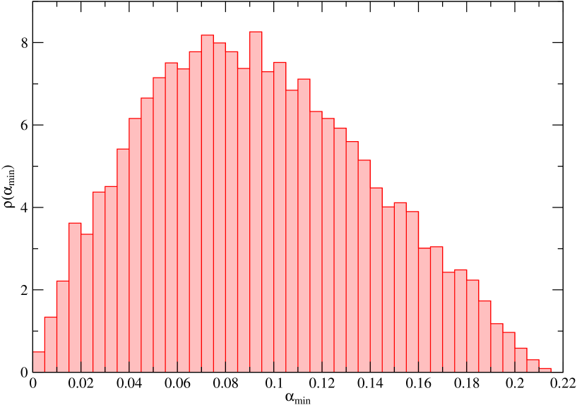
Figure 1: Distribution of $\alpha_{min}$ for uniformely distributed input parameters in the ranges $0.5<\rho<2$, $0.25<\lambda_{t,b}<1.25$, $2<k_{t}<3$, $0.75<k_{b}<1.5$, $0.75<\epsilon_{t}^{1,2}<2.5$, $0.1<\epsilon_{b}^{1,2}<0.45$.

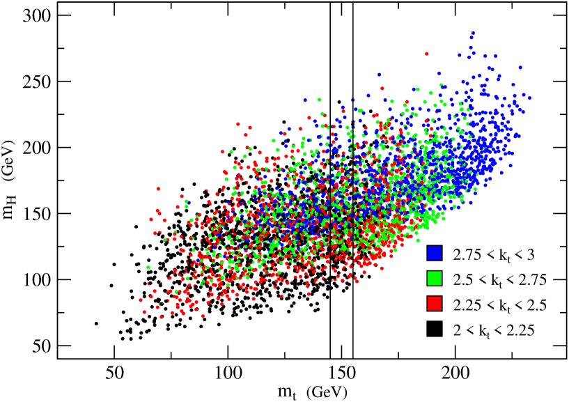
Figure 2: Higgs and top masses for points with $\alpha_{min}<0.05$. Different colors label different values of $k_{t}$. The region among the two vertical black lines corresponds to the physical top mass.

This can be seen from the histogram in fig. 2, which shows the distribution $\rho(\alpha_{min})$ for random (uniformly distributed) values of the input parameters, chosen in the ranges which give the correct order of magnitude for the top and bottom masses. We are neglecting the points with unbroken EW symmetry ($\alpha_{min}=0$), which are about half of the total.

From the effective potential we can determine the Higgs mass, which reads

$$m_{H}^{2}(\alpha_{min})=\displaystyle\frac{g_{5}^{2}R}{8\pi}\,\frac{\partial^{2}V}{\partial\alpha^{2}}\bigg{|}_{\alpha=\alpha_{min}}\;.$$ (2.14)

In fig. 2 the Higgs mass is plotted versus the top one and different colors label different ranges of the input parameter $k_{t}$. We see how realistic values of $m_{t}$ can be obtained already for $k_{t}=2$. The two vertical black lines in fig. 2 identify the region of physical top mass. This is taken to be around 150 GeV, which is the value one gets by running the physical top mass using the SM RGE equations up to the scale $1/R$. From fig. 2 we see that the Higgs mass lies in the $[100,200]$ GeV range. It is then significantly lighter than what found in [6].

2.2 Estimate of the Cut-off and Loop Corrections

The model presented here, as any 5D gauge theory, is non-renormalizable and hence has a definite energy range of validity, out of which the theory enters in a strong coupling uncontrolled regime. It is fundamental to have an estimate of the maximum energy $\Lambda$ which we can probe using our effective 5D Lagrangian (2.4). First of all, we have to check that $\Lambda$ is significantly above the compactification scale $1/R$, otherwise the 5D model has no perturbative range of applicability. Once the order of magnitude of $\Lambda$ is known, we can also estimate the natural values of the parameters entering in the Lagrangian (2.4). We define $\Lambda$ as the energy scale at which the one-loop vacuum polarization corrections for the various gauge field propagators is of order of the tree–level terms. This can be taken as a signal of the beginning of a strong coupling regime. The relevant gauge fields are those of $SU(3)_{i,s}$ and $SU(3)_{w}$, the abelian ones associated to $U(1)_{1,2}$ typically giving smaller corrections for any reasonable choice of $\rho^{2}$. Due to the Lorentz violation, however, the transverse ($A_{\mu}$) and longitudinal ($A_{5}$) gauge bosons couple differently between themselves and with matter, so that they should be treated separately. We have computed the one-loop vacuum polarizations neglecting the effect of the compactification, which should give small finite size effects, using a Pauli-Villars (PV) regularization in a non compact 5D space. We denote by $\Lambda_{s}^{(\mu)}$, $\Lambda_{s}^{(5)}$, $\Lambda_{w}^{(\mu)}$ and $\Lambda_{w}^{(5)}$ the resulting cut-offs (due to the mirror symmetry, the cut-offs associated to the two $SU(3)_{s}$ gauge groups coincide). A reasonable approximation is to assume that the gauge contribution is approximately of the same order as that of the fermions associated to the first two generations. In this case, by taking $k_{t}\simeq 2\div 3$, $k_{b}\simeq 1$, which are the typical phenomenological values, we get

$$(\Lambda^{(\mu)}_{s}R)\frac{\alpha_{s}}{6}\frac{1}{2}\Big{(}\frac{12}{k_{t}}+\frac{24}{k_{b}}\Big{)}\sim 1\ \ \Rightarrow\ \ \Lambda^{(\mu)}_{s} \sim\frac{6}{R}\,,$$

$$(\Lambda^{(5)}_{s}R)\frac{\alpha_{s}}{6}\frac{1}{2}\Big{(}12k_{t}+24k_{b}\Big{)}\sim\rho_{s}^{2}\ \ \Rightarrow\ \ \Lambda^{(5)}_{s} \sim\frac{3\rho^{2}_{s}}{R}\,,$$

$$(\Lambda^{(\mu)}_{w}R)\frac{\alpha_{w}}{6}\frac{1}{2}\Big{(}\frac{12}{k_{t}}+\frac{60}{k_{b}}\Big{)}\sim 1\ \ \Rightarrow\ \ \Lambda^{(\mu)}_{w} \sim\frac{5}{R}\,,$$

$$(\Lambda^{(5)}_{w}R)\frac{\alpha_{w}}{6}\frac{1}{2}\Big{(}12k_{t}+60k_{b}\Big{)}\sim 1\ \ \Rightarrow\ \ \Lambda^{(5)}_{w} \sim\frac{4}{R}\,.$$ (2.15)

As can be seen from eq. (2.15), $\Lambda^{(\mu)}$ and $\Lambda^{(5)}$ (both for the strong and weak coupling case) scale respectively as $k$ and $1/k$ in the Lorentz violating parameters. This is easily understood by noting that the loop factor scales as $1/k$ [6]. Thus $\Lambda^{(\mu)}\sim 1/\alpha\times k\sim k$ and $\Lambda^{(5)}\sim 1/(\alpha\,k^{2})\times k\sim 1/k$. Due to the group factor of the $SU(3)_{w}$ symmetric representation, the electroweak and strong interactions give comparable values for the cut-off. Independently of the strong interactions, the cut-off in the model is quite low: $\Lambda\sim 4/R$. The doubling of the fields due to the mirror symmetry has the strongest impact, since it decreases the electroweak cut-off estimate by a factor of $2$. As far as the Lorentz violation is concerned, we see that eq. (2.15) gives, for $k_{t}=k_{b}=\rho_{s}=1$, $\Lambda_{s}^{(5)}\sim 3/R$. In the absence of Lorentz breaking and mirror symmetry, therefore, the final cut-off would have been as low as $3/R$. Even though eq. (2.15) only provides an order–of–magnitude estimate, we can use it to place upper bounds on the allowed values of the Lorentz violating parameters $k_{t}$ and $k_{b}$. To ensure $\Lambda\gtrsim 4/R$, we impose $k_{t}\lesssim 3$ and $k_{b}\lesssim 1.2$.

Once we have an estimate for the value of the cut-off in the theory, we can also give an estimate of the natural size of the coefficients of the operators appearing in the Lagrangian (2.4). In particular, since we have neglected them, it is important to see the effect of the localized operators appearing in $\widehat{\cal{L}}_{0,\pi}$ when their coefficients are set to their natural value. At one–loop level, several localized kinetic operators are generated at the fixed-points. In the fermion sector, which appears to be the most relevant since it almost completely determines the Higgs potential, we have considered operators of the form

$$\widehat{\cal{L}}_{0,\pi}=\sum_{i}a^{i}_{0,\pi}\overline{\psi}^{i}i\,\raisebox{1.0pt}{$/$}\partial_{4}\,\psi^{i}\,,$$ (2.16)

where $\psi^{i}$ indicates here the components of the bulk fields which are non-vanishing at the $y=0$ or $y=\pi R$ boundaries. Such operators are logarithmically divergent at one-loop level and thus not very sensitive to the cut-off scale; anyhow, computing their coefficients $a^{i}_{0,\pi}$ using a PV regularization and setting $\Lambda\sim 4/R$, they turn out to be of order $10^{-3}R$. By including these terms in the full Lagrangian, we have verified that the shape of the effective potential, the Higgs and the fermion masses receive very small (of order per-mille) corrections. Localized operators can however sizeably affect the position of the minimum of the effective potential when it is tuned to assume small values. We will came back on this in subsection 3.1.

Finally, let us comment on the predictability of the Higgs mass at higher loops. Although finite at one-loop level, the Higgs mass will of course develop divergencies at higher orders, which require the introduction of various counterterms (see [25] for a two-loop computation of the Higgs mass term). The crucial point of identifying the Higgs with a Wilson line phase is the impossibility of having a local mass counterterm at any order in perturbation theory. This is true both in the Lorentz invariant and in the Lorentz breaking case. For this reason, the Higgs mass is computable. In the Lorentz invariant case, it weakly depends on the remaining counterterms needed to cancel divergencies loop by loop. In the Lorentz breaking case, the Higgs mass still weakly depends on higher-loop counterterms, with the exception of $\rho_{w}^{2}$, which is an arbitrary parameter directly entering in the Higgs mass formula. However, as we have already pointed out, $\rho_{w}$ always enters in any physical observable together with $R$, so that it can be rescaled by redefining the radius of compactification. Thanks to this property, the Higgs mass remains computable also in a Lorentz non-invariant scenario.

3 Phenomenological Bounds

A full and systematic analysis of all the new physical effects predicted by our theory is a quite complicated task, mainly because it mostly depends on how flavour is realized. For simplicity, we focus in the following on flavour and CP conserving new physics effects. Due to the strong constraints on flavor changing neutral currents (FCNC) and CP violation in the SM, this is a drastic but justified simplification, since flavour does not play an important role in our mechanism of EWSB. In fact we even did not discuss an explicit realization of it in our model (see however [5, 26] for possible realizations and [6] for an order of magnitude estimate of the bounds arising from FCNC). The only exception to this flavour universality is given by the third quark family, that has to be treated separately.

The analysis of flavour and CP conserving new physics effects requires in general the introduction of 18 dimension 6 operators in the SM to fit the data (see e.g. [12, 13]). It has recently been pointed out in [14] that, out of these 18 operators, only 10 are sensibly constrained. In a given basis (see [14] for details), $7$ of these operators are parametrized by the universal parameters $\widehat{S}$, $\widehat{T}$, $\widehat{U}$, $V$, $X$, $W$ and $Y$ introduced in [15] extending the usual $S,T,U$ basis [27]. They are defined in general in [15], starting from the inverse propagators $\Pi_{i,j}$ of the linear combinations of gauge bosons (not necessarily mass eigenstates of the Lagrangian) that couple to the SM fermions. As in the examples discussed in [15], in our model these gauge fields coincide with the “holographic” electroweak bosons which appear in eq. (2.12). The remaining 3 operators are parametrized by the distortion $\delta g_{b}$ (or the $\epsilon_{b}$ parameter [16]) of the $\widehat{Z}\,\overline{b}_{L}b_{L}$ coupling and other two parameters which describe the deviation of the up and down quark couplings to the $\widehat{Z}$ boson. As before, we put a hat superscript to distinguish the holographic field from its corresponding 5D field or mass eigenstate. Due to the way in which SM fermions couple in our model, the later two parameters are totally negligible. Being all light fermions almost completely localized at $y=0$ (see fig. 7 in appendix B for a quantitative idea of this effect), their couplings with the SM gauge fields are universal and not significantly distorted. As in other models based on extra dimensions [28, 29, 7], a possible exception is the bottom quark coupling (the top even more, but its coupling to the $\widehat{Z}$ is at the moment practically unconstrained), which is instead typically distorted by new physics. In the original version of our model considered in [6], indeed, $\delta g_{b}$ turned out to give one of the strongest constraints on the model. As anticipated before and as we will now see in some detail, the simple idea of reversing the mixing of the localized bottom and top quark with respect to [6] strongly reduces $\delta g_{b}$.

To be more precise, the distortion of the $\widehat{Z}\,\overline{b}_{L}b_{L}$ coupling is due to two effects. One of those is the mass–term mixing of the $b_{L}$ with the KK tower of the $SU(2)_{w}$ triplet and singlet fermions coming from the bulk field in the rep. $\bf 6$ of $SU(3)_{w}$. The second distortion is a consequence of the delocalization of $b_{L}$, which then also couples to gauge bosons components orthogonal to $\widehat{Z}$. Both effects are proportional to the mixing parameters $\epsilon_{1}^{t,b}$. Interestingly enough, at leading order in $\alpha=m_{W}R$ , the former distortion exactly vanishes in the (very good) approximation of neglecting the bottom mass. This can be understood by noting that the $b_{L}$ mixes with the component of an $SU(2)_{w}$ triplet which has $T_{3}=-1$ and with a singlet ($T_{3}=0$). The mixing with the triplet state leads to an increase (in magnitude) of $g_{b}$, whereas the singlet makes it decrease. The two effects turn out to exactly compensate each other. The distortion due to the delocalization of $b_{L}$ is instead non-vanishing. An explicit computation along the lines of the one reported in appendix A gives, at leading order in $\alpha$:

$$\delta g_{b}=g_{b}-g_{b}^{SM}=\frac{g_{b}^{SM}\pi^{2}\alpha^{2}}{4Z_{1}^{b}\cos^{2}\theta_{W}}\sum_{i=t,b}\frac{{\epsilon_{1}^{i}}^{2}}{\lambda_{i}^{2}}F\left(\frac{\lambda_{i}}{k_{i}}\right)\,,$$ (3.1)

where $F(x)$ is defined in eq. (A.8) and $Z_{1}^{b}$ is the wave function normalization factor needed to canonically normalize the $b_{L}$ field, defined in the equation (2.18) of [6] (recall $t\leftrightarrow b$ with respect to [6]). We have verified the validity of eq. (3.1) by computing it both holographically and from a more direct KK analysis. In the latter case, the distortion is caused by the KK tower of the $A_{X}$ gauge field, which mixes to the lowest mass eigenstate of the $Z$ boson and couples to $b_{L}$ in the bulk. It is worth to notice that the two results agree completely, but only when one sets the $\widehat{Z}$ boson on-shell in the holographic approach, as it should be done. This result is expected, if one considers that at the pole, the $\widehat{Z}$ gauge boson is totally given by its lowest mass eigenstate $Z$. In the holographic approach, as shown in appendix A in a toy example, one would find $\delta g_{b}$ to be identically zero if it is computed at zero momentum. Since $F(x)$ is a positive function, $\delta g_{b}<0$. In the typical range of parameters of phenomenological interest, $-\delta g_{b}\lesssim 2\alpha^{2}$ and it comfortably lies inside the experimentally allowed region (at $1\ \sigma$ form the central value) if $\alpha\lesssim 3\times 10^{-2}$. As we will now discuss, stronger bounds on $\alpha$ arise from universal corrections and non-universal corrections to $Z\overline{b}_{L}b_{L}$ can be neglected in our global fit.

We are left with the 7 parameters $\widehat{S}$, $\widehat{T}$, $\widehat{U}$, $V$, $X$, $W$ and $Y$. From the inverse gauge propagators $\Pi_{i,j}$ in eq. (2.12), one easily finds, at tree–level and at leading order in $\alpha$,

$$\left\{\begin{array}[]{l}\widehat{S}=\displaystyle\frac{2}{3}\alpha^{2}\pi^{2}\\ \rule{0.0pt}{15.00002pt}\widehat{T}=\alpha^{2}\pi^{2}\\ \rule{0.0pt}{15.00002pt}\widehat{U}=\displaystyle-\frac{2}{3}\alpha^{4}\pi^{4}\\ \rule{0.0pt}{15.00002pt}V=\displaystyle\frac{14}{45}\alpha^{6}\pi^{6}\end{array}\right.\,,\hskip 35.00005pt\left\{\begin{array}[]{l}X=\displaystyle\frac{14}{45}\tan(\theta_{w})\alpha^{4}\pi^{4}\\ \rule{0.0pt}{22.50003pt}Y=\displaystyle\frac{\rho^{2}\sin^{2}(\theta_{w})+1+2\cos(2\theta_{w})}{9\rho^{2}\cos^{2}(\theta_{w})}\alpha^{2}\pi^{2}\\ \rule{0.0pt}{17.50002pt}W=\displaystyle\frac{1}{3}\alpha^{2}\pi^{2}\end{array}\right.\,.$$ (3.2)

Since $\alpha$ has to roughly be of order $10^{-2}$, we see from eq. (3.2) that the 3 parameters $\widehat{U}$, $V$ and $X$ are totally negligible. This is actually expected for any universal theory [15]. Notice that the universal parameters essentially depend only on $\alpha$, the other parameter entering is $\rho$, which affects only $Y$. We have verified that radiatively generated localized gauge kinetic terms give negligible effects in eq. (3.2) and can thus be consistently neglected.

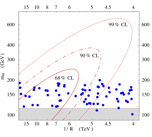
Figure 3: Constraints coming from a $\chi^{2}$ fit on the EWPT. The contours represent the allowed regions in the $(1/R,m_{H})$ plane at $68\%$, $90\%$ and $99\%$ confidence level (2 d.o.f.). The shaded band shows the experimentally excluded values for the Higgs mass ($m_{H}<115\ \rm GeV$). The blue dots represent the predictions of our model for different values of the microscopic parameters (only points with the correct top and bottom masses are plotted).

In fig. 3, we report the constraints on the Higgs mass and the compactification scale due to all electroweak flavour and CP conserving observables, obtained by a $\chi^{2}$ fit using the values in eq. (3.2). To better visualize the results, we fixed the value of the $\rho$ parameter to the Lorentz-symmetric value ($\rho=1$), hence we used a $\chi^{2}$ fit with 2 d.o.f. The fit essentially does not depend on $\rho$, as can be checked determining $\rho$ by a minimization of the $\chi^{2}$ function, which gives a plot which is almost indistinguishable from that reported in fig. 3. Due to their controversial interpretation (see e.g. [30]), we decided to exclude from the fit the NuTeV data. Nevertheless, we verified that the inclusion of such experiment leaves our results essentially unchanged. From fig. 3 one can extract a lower bound on the compactification scale $1/R\gtrsim 4-5\ \rm TeV$ (which corresponds to $\alpha\lesssim 0.016-0.02$) and an upper bound on the Higgs mass which varies from $m_{H}\lesssim 600\ \rm GeV$ at $1/R\sim 4\ \rm TeV$ to $m_{H}\lesssim 250\ \rm GeV$ for $1/R\gtrsim 10\ \rm TeV$. Notice that the values for $\widehat{S}$, $W$ and $Y$ (for $\rho=1$) found in eq. (3.2) are exactly those expected in a generic $5D$ theory with gauge bosons and Higgs in the bulk, as reported in eq. (20) of [15]. On the contrary, the $\widehat{T}$ parameter in eq. (3.2) is much bigger and is essentially due to the anomalous gauge field $A_{X}$. A heavy Higgs is allowed in our model because of this relatively high value of the $\widehat{T}$ parameter, which compensates the effects of a high Higgs mass.

Analyzing the models obtained by a random scan of the microscopic parameters, we found that the bound on the compactification scale can be easily fulfilled if a certain fine-tuning on the parameters is allowed. On the other hand, the bounds on the Higgs mass does not require any tuning.

3.1 Sensitivity, Predictivity and Fine-Tuning

As expected, the constraints arising from the electroweak observables require a quite stringent bound, $1/R\gtrsim 4.5\ \rm TeV$, on the size of the compactification scale. Differently from previously considered scenarios of GHU in flat space (see e.g. [5]), our model can satisfy such a bound (see fig. 3) for suitable choices of the microscopic input parameters. It is clear, however, that a certain cancellation (fine-tuning) must be at work in the Higgs potential to make its minimum $\alpha=m_{W}R$ as low as $0.018$.

The fine-tuning is commonly related [9] to the sensitivity of the observable ($\alpha$, in our case) with respect to variations of the microscopic input parameters. We define

$$C\equiv{\textrm{Max}}\left\{\left|\frac{\partial\log\alpha}{\partial\log I}\right|\right\}\,,$$ (3.3)

as the maximum of the logarithmic derivatives of $\alpha$ with respect to the various input parameters $I$. The fine-tuning, defined as $f=1/C$, is plotted in fig. 5 for the points which pass the $\chi^{2}$ test. For $1/R\sim 4.5\ \rm TeV$, the fine-tuning of our model is $1\,\%$.

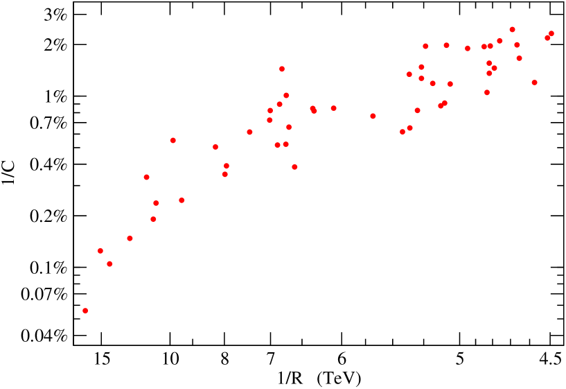
Figure 4: Inverse sensitivity for those points which pass the $\chi^{2}$ test.

Figure 5: Bayesian measure of the fine-tuning at fixed (black) and not fixed (red) top mass.

According to a more refined definition [10], the fine-tuning should be intended as an estimate of how unlike is a given value for an observable. This definition is not directly related to sensitivity, even though it reduces to $f=1/C$ in many common cases. In this framework, the fine-tuning is computed from the probability distribution $\rho(\alpha)$ of the output observable for “reasonable” distributions of the input microscopic parameters. One defines [10]

$$f=\frac{\alpha\rho(\alpha)}{\langle\alpha\rho(\alpha)\rangle}\,,$$ (3.4)

where $\langle\alpha\rho(\alpha)\rangle=\int d\alpha\,\alpha\left[\rho(\alpha)\right]^{2}$. The choice of the range of variation of the input parameters is the strongest ambiguity of the procedure, and must reflect physically well motivated assumptions. The distribution shown in fig. 2, which we will use, has been obtained with quite generic ranges, which however reflect our prejudice on the physical size of the top and bottom quark masses. Even though this does not make an important difference (see fig. 5), we can make our assumption more precise by further restricting to points in which the top (not the b, due to the lack of statistic) has the correct mass. The straightforward application of eq. (3.4) gives rise to the fine-tuning plot of fig. 5. At $1/R=4.5\ \rm TeV$ this prescription gives a fine-tuning of $10\%$. One could also relax the assumption of having EWSB. Since the fraction of points without EWSB is about one half of the total, one could argue, very roughly, that the resulting fine-tuning will increase of a factor two and be of order 5$\%$. This result strongly depends on the assumption we did on the fermion mass spectrum. In practice, what we observe is a certain correlation among the requirements of having a massive top and an high compactification scale, in the sense that points with massive top (and light b) also prefer to have small minima.

Independently on how we define the fine-tuning, however, the high value of $C$ at small $\alpha$ represents a problem by itself. The high sensitivity, indeed, makes $\alpha$ unstable against quantum corrections or deformations of the Lagrangian with the inclusion of new (small) operators. As described in section 2.2, we have considered the effects on the observables of localized kinetic terms for bulk fermions. We found that such operators, which lead to very small corrections to all other observables considered in this paper, can completely destabilize the compactification scale at small $\alpha$. A similar effect is found when including in the effective potential the very small contributions which come from the light fermion families. For $\alpha\sim 0.02$ the corrections which come in both cases are of order $50\%$, so that the compactification radius is effectively not predicted in terms of the microscopic parameters of the model.

4 Conclusions

In this paper we presented a realistic GHU model on a flat 5-dimensional orbifold $S^{1}/{\bf Z}_{2}$. The model is based on the one outlined in [6], in which an explicit breaking of the $SO(4,1)$ Lorentz symmetry down to the usual 4-dimensional Lorentz group $SO(3,1)$ was advocated in order to overcome some of the most worrisome common problems of GHU models on flat space.

The main new feature of the present model is the presence of a ${\bf Z}_{2}$ “mirror symmetry”, which essentially consists in a doubling of part of the bulk fields, contributing to a reduction of the fine-tuning. It also allows to have a stable boson at the $\rm TeV$ scale, which could prove to be a viable dark matter candidate. We have also shown how, due to a suitable choice of the bulk fermion quantum numbers, the deviations from the $Z\overline{b}_{L}b_{L}$ SM coupling can be made totally negligible. The new physics effects can be encoded in the 4 parameters $\widehat{S}$, $\widehat{T}$, $W$ and $Y$ defined in [15], and thus our model effectively belongs to the class of universal theories. From a combined fit, we derived a lower bound on the compactification scale $1/R\gtrsim 4\ \rm TeV$ with allowed (although never reached, see fig. 3) Higgs masses up to 600 GeV. Our model is compatible with the experimental constraints if a certain tuning in the parameter space, of order of a few $\%$, is allowed. Such a fine-tuning is certainly acceptable, but it is nevertheless still too high to claim that our model represents a solution to the little hierarchy problem. However, it should be emphasized that the fine-tuning we get is of the same order of that found in the MSSM.

Appendix A The “Holographic” Approach

Deriving $4D$ effective theories from $5D$ models is usually done by integrating out the massive KK eigenstates, keeping the lightest states of the KK towers as effective degrees of freedom. When the extra space has a boundary at $y=0$, an alternative and useful “holographic” possibility is to use the boundary values $\widehat{\Phi}(x)=\Phi(x,0)$ of the $5D$ fields as effective degrees of freedom and to integrate out all the fields components $\Phi(x,y)$ with $y\neq 0$ [19]. As long as $\Phi(x,0)$ has a non-vanishing component of the light mode of the KK tower associated to $\Phi(x,y)$, the holographic and KK approaches are completely equivalent. In warped 5D models, such a prescription closely resembles the one defined by the AdS/CFT correspondence [31], where roughly speaking $\widehat{\Phi}(x)$ is the source of a CFT operator and $\Phi(x,y)$ is the corresponding AdS bulk field. Although in flat space such interpretation is missing, it has been emphasized in [19] that it is nevertheless a useful technical tool to analyze various properties of 5D theories. The holographic approach, in this paper, has been used to perform the global fit to EW observables. Along the lines of [15], it significantly simplifies the analysis.

We think it might be useful to collect here a few technical details on how to use this approach in our particular context. To keep the discussion as clear as possible, and to emphasize the key points, we consider in this appendix a simple $5D$ Lorentz invariant model on a segment of length $L$, which resembles some aspects of our construction. Let $A_{M}$ be an $U(1)$ bulk gauge field, $\psi$ and $\chi$ a couple of bulk charged fermions and $q_{R}$ a chiral $4D$ fermion localized at $y=0$, which mixes with $\psi_{L}$. The gauge field components $A_{\mu}$ and $A_{5}$ satisfy respectively Neumann amd Dirichlet boundary conditions at $y=L$, whereas for the fermions we have $\psi_{R}(L)=\chi_{L}(L)=0$. For what concerns the bosonic fields, boundary conditions at $y=0$ are simply imposed by the choice of the dynamical holographic fields to be retained. The holographic approach to fermions is a bit more complicated since one has to modify the action by introducing suitable localized mass-terms [20]. With the convention $\gamma^{5}\psi_{L}=+\psi_{L}$, the action reads

$$S=\int_{0}^{L}\!dy \!d^{4}x\bigg{\{}-\frac{1}{4}F_{MN}F^{MN}+\Big{[}\frac{1}{2}(\overline{\psi}i\hskip 3.0pt\raisebox{1.0pt}{$/$}D_{5}\psi+\overline{\chi}i\hskip 3.0pt\raisebox{1.0pt}{$/$}D_{5}\chi)-M\overline{\chi}\psi+h.c.\Big{]}\bigg{\}}$$

$$+\int\!d^{4}x \frac{1}{2}\Big{[}\overline{q}_{R}i\hskip 3.0pt\raisebox{1.0pt}{$/$}D_{4}q_{R}+e\,\overline{q}_{R}\psi_{L}(0)+e\,\overline{\psi}_{L}(0)q_{R}+\overline{\psi}(0)\psi(0)-\overline{\chi}(0)\chi(0)\Big{]}\,,$$ (A.1)

and one can check that, by performing generic variation of the bulk fermion fields, the boundary conditions $\psi_{R}(0)=-e/2\,q_{R}$ and $\chi_{L}(0)=0$ automatically arise as equations of motion. The field which we will retain are $\widehat{A}_{\mu}=A_{\mu}(0)$ and $q_{R}$. Integrating out at tree-level the remaining degrees of freedom is equivalent to solve their equation of motion with fixed holographic fields ($\delta\widehat{A}_{\mu}=\delta q_{R}=0$ in the action variation) and to plug the solution back into the action. Varying eq. (A.1) with the holographic prescription simply gives the standard $5D$ Dirac and Maxwell equations plus the above mentioned boundary conditions for the fermions.

It is useful to adopt a mixed momentum-space basis $\phi(p,y)$ for the fields. In the unitary gauge $A_{5}$ vanishes and the longitudinal component of $A_{\mu}$ is decoupled, while the equations for the transverse part $A_{\mu}^{t}={\cal P}_{\mu\nu}A^{\nu}$ (${\cal P}_{\mu\nu}=\eta_{\mu\nu}-p_{\mu}p_{\nu}/p^{2}$) reduce to $(p^{2}+\partial_{y}^{2})A_{\mu}^{t}(p,y)=0$. Imposing the boundary condition $\partial_{y}A_{\mu}(L)=0$, one easily gets

$$A_{\mu}(p,y)=\frac{\cos\left[p(L-y)\right]}{\cos\left[p\,L\right]}\widehat{A}_{\mu}^{t}(p)\,,$$ (A.2)

where $p=\sqrt{p^{\mu}p_{\mu}}$. One proceeds analogously for fermions. It is a simple exercise, given the boundary conditions at $y=L$, to determine $\psi(p,y)$ and $\chi(p,y)$ in terms of $q_{R}$. One gets

$$\psi_{R} = -\frac{e}{2}\,\frac{\sin\left[\omega(L-y)\right]}{\sin\left[\omega\,L\right]}\,q_{R}\,;\;\;\;\;\;\psi_{L}=-\frac{e}{2}\,\frac{\cos\left[\omega(L-y)\right]}{\omega\sin\left[\omega\,L\right]}\,\raisebox{1.0pt}{$/$}p\,q_{R}\,;$$

$$\chi_{L} = 0\,;\;\;\;\;\;\;\;\;\;\;\;\;\;\;\;\;\;\;\;\;\;\;\;\;\;\;\;\;\;\;\;\;\;\;\;\chi_{R}=-\frac{e}{2}\,\frac{\cos\left[\omega(L-y)\right]}{\omega\sin\left[\omega\,L\right]}\,M\,q_{R}\,;$$ (A.3)

where $\omega=\sqrt{p^{2}-M^{2}}$. Plugging back the solutions (A.2) and (A.3) into the action (A.1), we can get the holographic Lagrangian. At quadratic level

$${\cal L}_{holo}=-\frac{1}{2}\Pi(p)\widehat{A}_{\mu}^{t}\widehat{A}^{t\,\mu}+\frac{1}{2}Z_{q}\overline{q}_{R}\,\raisebox{1.0pt}{$/$}p_{4}\,q_{R}\,,$$ (A.4)

where we defined

$$\Pi(p)=p\tan pL,\ \ \ Z_{q}=1-\frac{e^{2}}{2}\,\frac{\cot\omega L}{\omega}\,.$$ (A.5)

The holographic procedure can also be used to study interaction terms. Again, one has simply to substitute into the action (A.1) the solutions (A.2) and (A.3). It is useful to see how this works by computing the distortion to the $U(1)$ gauge coupling $g$ of $q_{R}$ to $\widehat{A}_{\mu}$ due to the massive modes. This interaction is encoded in the following Lagrangian term:

$${\cal L}^{(3)}= g\int^{L}_{0}\!dy\Big{[}\overline{\psi}(p+q,y)\hskip 3.0pt\raisebox{1.0pt}{$/$}A(q,y)\psi(p,y)+\overline{\chi}(p+q,y)\hskip 3.0pt\raisebox{1.0pt}{$/$}A(q,y)\chi(p,y)\Big{]}$$ (A.6)

$$+\,\frac{g}{2}\,\overline{q}_{R}(p+q)\widehat{\hskip 3.0pt}\raisebox{1.0pt}{$/$}A(q)q_{R}(p)\,.$$

In order to simplify our computation, let us consider the kinematic configuration in which the fermion is on-shell, $p^{2}=(p+q)^{2}=0$, and $q^{2}=\mu^{2}\ll M^{2}$. By direct substitution and after a bit of algebra, one gets the following cubic interaction, up to terms of order $\mu^{2}/M^{2}$:

$${\cal L}^{(3)}= \frac{g}{2}\Big{[}Z_{q}+\frac{e^{2}\,\mu^{2}}{8M^{2}}F(ML)\Big{]}\overline{q}_{R}(p+q)\widehat{\hskip 3.0pt}\raisebox{1.0pt}{$/$}A^{t}(q)q_{R}(p)\,,$$ (A.7)

where $Z_{q}$ is computed at zero momentum and we have defined

$$F(x)\equiv 1-\frac{1}{x}\coth x+\coth^{2}x\,.$$ (A.8)

As expected, the form of the interaction vertex at $\mu^{2}=0$ has precisely the same structure as the quadratic term in (A.4), as required by gauge invariance, which forbids any correction to $g$. At quadratic order in the gauge boson momentum, however, we get a correction

$$\delta g=\frac{g\,e^{2}}{8Z_{q}}\frac{\mu^{2}}{M^{2}}F(ML)\,.$$ (A.9)

Notice that eq. (A.9) coincides exactly with eq. (3.1), when fixing $\mu^{2}=m_{Z}^{2}$ and taking into account the SM coupling of the $b_{L}$. This is a further proof that no corrections arise in our model from the mixing of $b_{L}$ with fields with different isospin quantum numbers, the only effect being given by the partial delocalization of the field, resulting in couplings with the “massive” gauge fields $A_{\mu}(y)$, with $y\neq 0$.

The generalization to the non-abelian case and fields in different representations of the gauge group does not present any conceptual problem. When a Wilson line symmetry breaking occurs, like in our model, the most convenient thing to do is to go in a gauge in which the VEV for $A_{5}$ vanishes and the boundary conditions for the various fields are twisted at $y=0$. In this way, the effect of the twist simply amounts to a redefinition of the holographic fields, as discussed in section 2.1.

Appendix B Fermion Wave Functions

In this appendix we turn to the more standard analysis of the KK mass eigenstates and examine the wave functions of the fermions arising from the mixing of the bulk fields with the fields localized at $y=0$. The purpose of this analysis is to illustrate how much the SM fermions are localized in our model. As we will see, in fact, the top quark is not localized at all, whereas the bottom is only partially localized (see figs. 7 and 7). In order to simplify the discussion, we focus on the wave functions of right-handed singlets before EWSB. Left-handed localized fields are more involved since they couple to two different bulk fields, as shown in eq. (2.7).

The relevant quadratic Lagrangian describing the coupling of a localized right-handed fermion with the bulk fields is easily extracted from the full Lagrangian (2.4). It reads

$${\cal L} = \overline{\psi}(i\,\raisebox{1.0pt}{$/$}\partial_{4}-k\partial_{5}\gamma_{5})\psi+\overline{\widetilde{\psi}}(i\,\raisebox{1.0pt}{$/$}\partial_{4}-k\partial_{5}\gamma_{5}){\widetilde{\psi}}-M(\overline{\psi}{\widetilde{\psi}}+\overline{\widetilde{\psi}}\psi)$$ (B.1)

$$+\delta(y)[\overline{q}_{R}i\,\raisebox{1.0pt}{$/$}\partial_{4}q_{R}+e\overline{q}_{R}\psi_{L}+e\overline{\psi}_{L}q_{R}],$$

where $\psi$ and $\widetilde{\psi}$ are the singlet components of the periodic bulk fermions $\Psi^{t}_{+}$ and $\Psi_{+}^{b}$, respectively for $q_{R}=t_{R}$ and $q_{R}=b_{R}$. For simplicity of notation, we denote the bulk–to–boundary mixing parameter simply as $e$ in both cases. Due to the latter and the bulk mass $M$, the equations of motion for $\psi$, $\widetilde{\psi}$ and $q_{R}$ are all coupled with each other. The 4D KK mass eigenstates $\chi^{(n)}_{L,R}(x)$ of eq. (B.1) will then appear spread between the fields $\psi$, $\widetilde{\psi}$ and $q_{R}$. In other words, we expand the various fields as follows:

$$\left\{\begin{array}[]{l}q=\sum_{n}g_{n}\,\chi^{(n)}_{R}\,,\\ \psi_{L,R}=\sum_{n}f^{(n)}_{L,R}(y)\,\chi^{(n)}_{L,R}\,,\\ {\widetilde{\psi}}_{L,R}=\sum_{n}{\widetilde{f}}^{(n)}_{L,R}(y)\,\chi^{(n)}_{L,R}\,,\end{array}\right.$$ (B.2)

where $f^{(n)}_{L,R}(y)$ and ${\widetilde{f}}^{(n)}_{L,R}(y)$ are the wave functions along the fifth dimension and $g_{n}$ are constants. The $\chi$ fields satisfy the 4-dimensional Dirac equation

$$i\,\raisebox{1.0pt}{$/$}\partial_{4}\chi^{(n)}=m_{n}\chi^{(n)}\,,$$ (B.3)

where $\chi^{(n)}=\chi^{(n)}_{L}+\chi^{(n)}_{R}$, and $m_{n}$ is the mass of the $n^{\textrm{th}}$ state. By solving the equations of motion, one finds two distinct towers of eigenstates: an “unperturbed” tower with only massive fields and a “perturbed” one containing a right-handed massless field. We will also see how the mass spectra found here with the usual KK approach match with the one deduced from eq. (A.5) using the holographic approach.

The unperturbed tower

This tower has no component along the localized fields and is entirely build up with bulk fields. The wave functions are analytic over the whole covering space and the left-handed ones vanish at $y=0$. The mass levels are given by

$$m_{n}=\sqrt{M^{2}+\left(\frac{kn}{R}\right)^{2}}\,,$$ (B.4)

but with $n\geq 1$, without the $n=0$ mode. The corresponding wave functions are

$$\left\{\begin{array}[]{l}g_{n}=0\,,\\ f^{(n)}_{L}=0\,,\\ {\widetilde{f}}^{(n)}_{L}=\displaystyle\frac{1}{\sqrt{\pi R}}\sin\left(\frac{n}{R}y\right)\,,\end{array}\right.\qquad\left\{\begin{array}[]{l}f^{(n)}_{R}=\displaystyle\frac{M}{m_{n}\sqrt{\pi R}}\sin\left(\frac{n}{R}y\right)\,,\\ \rule{0.0pt}{17.50002pt}{\widetilde{f}}^{(n)}_{R}=\displaystyle\frac{nk/R}{m_{n}\sqrt{\pi R}}\cos\left(\frac{n}{R}y\right)\,.\end{array}\right.$$ (B.5)

Although $e$ does not explicitly appear in eqs. (B.4) and (B.5), its presence constrains the left-handed fields to vanish at $y=0$ and thus it indirectly enters in the above expressions. When $e$ vanishes, indeed, one recovers the usual mode $n=0$.

The perturbed tower

This tower is distorted by the coupling with the localized fields. Its massive levels are given by the solutions of the transcendental equation

$$\tan\left(\pi R\frac{\omega_{n}}{k}\right)=\frac{\epsilon^{2}}{\pi Rk\omega_{n}}\,,$$ (B.6)

where $\omega_{n}\equiv\sqrt{(m_{n}^{2}-M^{2})}$. Notice that the masses defined by eq. (B.6) exactly coincide, for $k=1$, with the zeroes of $Z_{q}$ in eq. (A.5). The mass equation has a tower of solutions with $m_{n}>M$, whose wave functions are

$$\left\{\begin{array}[]{l}f^{(n)}_{L}=\displaystyle-\frac{\epsilon m_{n}g_{n}}{\sqrt{2\pi R}k\omega_{n}}\frac{\cos\left((y-\pi R)\omega_{n}/k\right)}{\sin(\pi R\omega_{n}/k)}\,,\\ \rule{0.0pt}{17.50002pt}{\widetilde{f}}^{(n)}_{L}=0\,,\end{array}\right.\hskip 5.0pt\left\{\begin{array}[]{l}f^{(n)}_{R}=\displaystyle\frac{\epsilon g_{n}}{\sqrt{2\pi R}k}\frac{\sin\left((y-\pi R)\omega_{n}/k\right)}{\sin(\pi R\omega_{n}/k)}\,,\\ \rule{0.0pt}{17.50002pt}{\widetilde{f}}^{(n)}_{R}=\displaystyle-\frac{\epsilon Mg_{n}}{\sqrt{2\pi R}k\omega_{n}}\frac{\cos\left((y-\pi R)\omega_{n}/k\right)}{\sin(\pi R\omega_{n}/k)}\,,\end{array}\right.$$ (B.7)

The constants $g_{n}$ in eq. (B.2) are determined by imposing the canonical normalization of the 4D fields. One gets

$$g_{n}=\left[1+\frac{\epsilon^{2}}{2\pi Rk^{2}\omega_{n}^{2}}\left(\frac{\pi Rm_{n}^{2}}{\sin^{2}(\pi R\omega_{n}/k)}+k\frac{M^{2}-\omega_{n}^{2}}{\omega_{n}}\cot(\pi R\omega_{n}/k)\right)\right]^{-1/2}\,.$$ (B.8)

Notice that some care has to be used in taking the limit $\epsilon\rightarrow 0$ in the above expressions, since one encounters apparently ill-defined expressions in eqs. (B.7) and (B.8).

The zero mode

The zero mode is of particular interest, being identified with a SM field. Its wave function is

$$\left\{\begin{array}[]{l}f^{(0)}_{L}=0\,,\\ \rule{0.0pt}{25.00003pt}{\widetilde{f}}^{(0)}_{L}=0\,,\end{array}\right.\qquad\qquad\left\{\begin{array}[]{l}f^{(0)}_{R}=\displaystyle\frac{\epsilon g_{0}}{\sqrt{2\pi R}k}\frac{\sinh\left((y-\pi R)M/k\right)}{\sinh(\pi RM/k)}\,,\\ \rule{0.0pt}{17.50002pt}{\widetilde{f}}^{(0)}_{R}=\displaystyle\frac{\epsilon g_{0}}{\sqrt{2\pi R}k}\frac{\cosh\left((y-\pi R)M/k\right)}{\sinh(\pi RM/k)}\,,\end{array}\right.$$ (B.9)

where again $g_{0}$ is determined by the normalization conditions and equals

$$g_{0}=\left[1+\frac{\epsilon^{2}}{\pi RMk}\coth(\pi RM/k)\right]^{-1/2}\,.$$ (B.10)

The constant $g_{0}$ indicates how much of the zero mode field is composed of the localized field. When $\epsilon\ll 1$ and $g_{0}\sim 1$, as expected, the wave function of the massless state is mostly given by the localized field, the bulk components (B.9) being proportional to $\epsilon$ and thus small. On the contrary, for large mixing $\epsilon\gg 1$, one has $g_{0}\ll 1$ and the localized field is completely “dissolved” into the bulk degrees of freedom. In the latter case, then, the localization of the $\psi_{R}$ and ${\widetilde{\psi}}_{R}$ components of the zero mode is essentially determined by the adimensional quantity $\pi RM/k$. The bulk wave functions at $y=\pi R$ are suppressed by a factor $\exp(-\pi RM/k)$ with respect to their value at $y=0$ so that, independently of $\epsilon$, for large values of $\pi RM/k$ the chiral field is still localized at $y=0$.

Summarizing, the zero mode is localized at $y=0$ for small mixing with the bulk fields and arbitrary bulk masses, or for large bulk masses and arbitrary mixing. The requirement of having the correct top mass after EWSB implies a large mixing and a small bulk mass, giving rise to a delocalized top wave function.

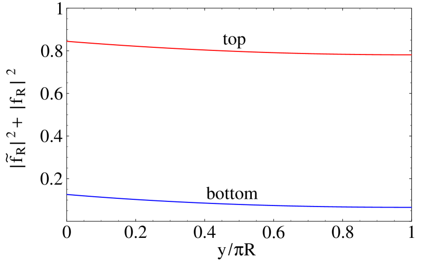
Figure 6: Top (red) and bottom (blue) quark wave function profiles (right handed components). The areas below the lines represent the amount of the delocalized part of the fields.

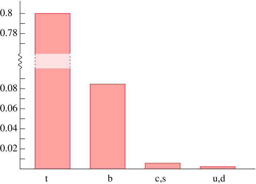
Figure 7: Delocalized part of the quark wave functions. The fraction of bulk wave function is shown for the various quarks.

In fig. 7 we illustrate the wave function profiles of the right-handed top and bottom quark components for typical acceptable values of input parameters, before EWSB.

The mass spectrum and fermion wave functions for the antiperiodic fermions $\Psi_{-}$ and $\widetilde{\Psi}_{-}$ is straightforward, since they do not couple with the localized fields. Their wave functions can be written as

$$\left\{\begin{array}[]{l}f^{(n)}_{L}=\displaystyle\frac{1}{\sqrt{2\pi R}}\cos\left(\frac{n+1/2}{R}y\right)\,,\\ {\widetilde{f}}^{(n)}_{L}=\displaystyle\frac{\mp 1}{\sqrt{2\pi R}}\sin\left(\frac{n+1/2}{R}y\right)\,,\end{array}\right.\left\{\begin{array}[]{l}f^{(n)}_{R}=\displaystyle\frac{\mp M-(n+1/2)k/R}{m_{n}\sqrt{2\pi R}}\sin\left(\frac{n+1/2}{R}y\right)\,,\\ \rule{0.0pt}{17.50002pt}{\widetilde{f}}^{(n)}_{R}=\displaystyle\frac{M\mp(n+1/2)k/R}{m_{n}\sqrt{2\pi R}}\cos\left(\frac{n+1/2}{R}y\right)\,,\end{array}\right.$$ (B.11)

where $n\geq 0$ and $\pm$ stands for the two towers of mass eigenstates, both with masses given by

$$m_{n}=\sqrt{M^{2}+\left(\frac{k(n+1/2)}{R}\right)^{2}}\,.$$ (B.12)

After EWSB, all above relations are clearly modified by $O(\alpha)$ effects. In particular, a small fraction of the SM fields is now spread also among the bulk fermion components whose mixing were forbidden by $SU(2)_{L}\times U(1)_{Y}$ symmetry. We do not write the modification to the mass formula (B.6) for the deformed tower, the form of which can be deduced from the zeroes of the integrand of eqs. (2.15) and (2.16) of [6], with the replacement $t\leftrightarrow b$.

References

- [1]
- [2] I. Antoniadis, Phys. Lett. B 246 (1990) 377.
-
[3]
D. B. Fairlie,
Phys. Lett. B 82 (1979) 97;
J. Phys. G 5 (1979) L55;
N. S. Manton, Nucl. Phys. B 158 (1979) 141;
P. Forgacs, N. S. Manton, Commun. Math. Phys. 72 (1980) 15;
S. Randjbar-Daemi, A. Salam, J. Strathdee, Nucl. Phys. B 214 (1983) 491;
N. V. Krasnikov, Phys. Lett. B 273 (1991) 246;
H. Hatanaka, T. Inami, C. Lim, Mod. Phys. Lett. A 13 (1998) 2601 [hep-th/9805067]. -
[4]
G. R. Dvali, S. Randjbar-Daemi, R. Tabbash,
Phys. Rev. D 65 (2002) 064021
[hep-ph/0102307];
L. J. Hall, Y. Nomura, D. R. Smith, Nucl. Phys. B 639 (2002) 307 [hep-ph/0107331];
I. Antoniadis, K. Benakli, M. Quiros, New J. Phys. 3 (2001) 20 [hep-th/0108005];
M. Kubo, C. S. Lim and H. Yamashita, Mod. Phys. Lett. A 17 (2002) 2249 [arXiv:hep-ph/0111327];
C. Csaki, C. Grojean, H. Murayama, Phys. Rev. D 67 (2003) 085012 [hep-ph/0210133];
G. Burdman, Y. Nomura, Nucl. Phys. B 656 (2003) 3 [hep-ph/0210257];
N. Haba, M. Harada, Y. Hosotani and Y. Kawamura, Nucl. Phys. B 657 (2003) 169 [Erratum-ibid. B 669 (2003) 381] [arXiv:hep-ph/0212035];
N. Haba, Y. Shimizu, Phys. Rev. D 67 (2003) 095001 [hep-ph/0212166];
K. w. Choi et al., JHEP 0402 (2004) 037 [arXiv:hep-ph/0312178];
I. Gogoladze, Y. Mimura, S. Nandi, Phys. Lett. B 560 (2003) 204 [hep-ph/0301014]; ibid. 562 (2003) 307 [hep-ph/0302176]; Phys. Rev. D 69 (2004) 075006 [arXiv:hep-ph/0311127].
C. A. Scrucca, M. Serone, L. Silvestrini and A. Wulzer, JHEP 0402 (2004) 049 [arXiv:hep-th/0312267];
N. Haba, Y. Hosotani, Y. Kawamura and T. Yamashita, Phys. Rev. D 70 (2004) 015010 [arXiv:hep-ph/0401183];
C. Biggio and M. Quiros, Nucl. Phys. B 703 (2004) 199 [arXiv:hep-ph/0407348];
K. y. Oda and A. Weiler, Phys. Lett. B 606 (2005) 408 [arXiv:hep-ph/0410061];
Y. Hosotani and M. Mabe, Phys. Lett. B 615 (2005) 257 [arXiv:hep-ph/0503020];
A. Aranda and J. L. Diaz-Cruz, Phys. Lett. B 633 (2006) 591 [arXiv:hep-ph/0510138];
G. Cacciapaglia, C. Csaki and S. C. Park, JHEP 0603 (2006) 099 [arXiv:hep-ph/0510366]. - [5] C. A. Scrucca, M. Serone, L. Silvestrini, Nucl. Phys. B 669 (2003) 128 [hep-ph/0304220].
- [6] G. Panico, M. Serone and A. Wulzer, Nucl. Phys. B 739 (2006) 186 [arXiv:hep-ph/0510373].
- [7] K. Agashe, R. Contino and A. Pomarol, Nucl. Phys. B 719 (2005) 165 [arXiv:hep-ph/0412089]; K. Agashe and R. Contino, Nucl. Phys. B 742 (2006) 59 [arXiv:hep-ph/0510164].
- [8] B. Grzadkowski and J. Wudka, “5-dimensional difficulties of gauge-Higgs unifications,” arXiv:hep-ph/0604225.
- [9] R. Barbieri and G. F. Giudice, Nucl. Phys. B 306 (1988) 63.
- [10] G. W. Anderson and D. J. Castano, Phys. Lett. B 347 (1995) 300 [arXiv:hep-ph/9409419].
- [11] G. Servant and T. M. P. Tait, Nucl. Phys. B 650 (2003) 391 [arXiv:hep-ph/0206071].
- [12] Z. Han and W. Skiba, Phys. Rev. D 71 (2005) 075009 [arXiv:hep-ph/0412166].
- [13] C. Grojean, W. Skiba and J. Terning, Phys. Rev. D 73 (2006) 075008 [arXiv:hep-ph/0602154].
- [14] G. Cacciapaglia, C. Csaki, G. Marandella and A. Strumia, “The minimal set of electroweak precision parameters,” arXiv:hep-ph/0604111.
- [15] R. Barbieri, A. Pomarol, R. Rattazzi and A. Strumia, Nucl. Phys. B 703, 127 (2004) [arXiv:hep-ph/0405040].
- [16] G. Altarelli, R. Barbieri and F. Caravaglios, Nucl. Phys. B 405 (1993) 3.
- [17] I. Gogoladze and C. Macesanu, “Precision electroweak constraints on Universal Extra Dimensions revisited,” arXiv:hep-ph/0605207.
- [18] T. Appelquist, H. C. Cheng and B. A. Dobrescu, Phys. Rev. D 64 (2001) 035002 [arXiv:hep-ph/0012100].
- [19] R. Barbieri, A. Pomarol and R. Rattazzi, Phys. Lett. B 591 (2004) 141 [arXiv:hep-ph/0310285].
- [20] R. Contino and A. Pomarol, JHEP 0411 (2004) 058 [arXiv:hep-th/0406257].
- [21] Y. Hosotani, Phys. Lett. B 126 (1983) 309; ibid. 129 (1983) 193; Ann. Phys. 190 (1989) 233.
- [22] F. del Aguila, M. Perez-Victoria and J. Santiago, JHEP 0302 (2003) 051 [arXiv:hep-th/0302023].
- [23] F. del Aguila, M. Perez-Victoria and J. Santiago, “Effective description of brane terms in extra dimensions,” arXiv:hep-ph/0601222.
- [24] A. Lewandowski and R. Sundrum, Phys. Rev. D 65 (2002) 044003 [arXiv:hep-th/0108025].
- [25] N. Maru and T. Yamashita, “Two-loop calculation of Higgs mass in gauge-Higgs unification: 5D massless QED compactified on S**1,” arXiv:hep-ph/0603237.
- [26] G. Martinelli, M. Salvatori, C. A. Scrucca and L. Silvestrini, JHEP 0510 (2005) 037 [arXiv:hep-ph/0503179].
- [27] M. E. Peskin and T. Takeuchi, Phys. Rev. D 46 (1992) 381.
- [28] K. Agashe, A. Delgado, M. J. May and R. Sundrum, JHEP 0308 (2003) 050 [arXiv:hep-ph/0308036].
-
[29]
G. Burdman and Y. Nomura,
Phys. Rev. D 69 (2004) 115013
[arXiv:hep-ph/0312247];
G. Cacciapaglia, C. Csaki, C. Grojean and J. Terning, Phys. Rev. D 71 (2005) 035015 [arXiv:hep-ph/0409126]. - [30] G. Altarelli and M. W. Grunewald, Phys. Rept. 403-404 (2004) 189 [arXiv:hep-ph/0404165].
-
[31]
J. M. Maldacena,
Adv. Theor. Math. Phys. 2 (1998) 231
[Int. J. Theor. Phys. 38 (1999) 1113]
[arXiv:hep-th/9711200];
S. S. Gubser, I. R. Klebanov and A. M. Polyakov, Phys. Lett. B 428 (1998) 105 [arXiv:hep-th/9802109];
E. Witten, Adv. Theor. Math. Phys. 2 (1998) 253 [arXiv:hep-th/9802150].