Study of the Change from Walking to Non-Walking Behavior
in a Vectorial Gauge Theory as a Function of $N_{f}$

Abstract

We study a vectorial gauge theory with gauge group ${\rm SU}(N_{c})$ and a variable number, $N_{f}$, of massless fermions in the fundamental representation of this group. Using approximate solutions of Schwinger-Dyson and Bethe-Salpeter equations, we calculate meson masses and investigate how these depend on $N_{f}$. We focus on the range of $N_{f}$ extending from near the boundary with a non-Abelian Coulomb phase, where the theory exhibits a slowly running (“walking”) gauge coupling, toward smaller values where the theory has non-walking behavior. Our results include determinations of the masses of the lowest-lying flavor-adjoint mesons with $J^{PC}=0^{-+}$, $1^{--}$, $0^{++}$, and $1^{++}$ (the generalized $\pi$, $\rho$, $a_{0}$, and $a_{1}$). Related results are given for flavor-singlet mesons and for the generalization of $f_{\pi}$. These results give insight into the change from walking to non-walking behavior in a gauge theory, as a function of $N_{f}$.

I Introduction

We consider a $(3+1)$-dimensional vectorial gauge theory (at zero temperature and chemical potential) with the gauge group SU($N_{c}$) and $N_{f}$ massless fermions transforming according to the fundamental representation of this group. For $N_{c}=3$, if one took $N_{f}=2$, this would be an approximation to actual quantum chromodynamics (QCD) with just the $u$ and $d$ quarks, since their current quark masses are small compared with the scale $\Lambda_{QCD}\simeq 400$ MeV. We restrict here to the range $N_{f}<(11/2)N_{c}$ for which the theory is asymptotically free. An analysis using the two-loop beta function and Schwinger-Dyson equation (reviewed below) leads to the inference that for $N_{f}$ in this range, the theory includes two phases: (i) for $0\leq N_{f}\leq N_{f,cr}$ a phase with confinement and spontaneous chiral symmetry breaking (S$\chi$SB); and (ii) for $N_{f,cr}\leq N_{f}\leq(11/2)N_{c}$ a non-Abelian Coulomb phase with no confinement or spontaneous chiral symmetry breaking. We shall refer to $N_{f,cr}$, the critical value of $N_{f}$, as the boundary of the non-Abelian Coulomb (conformal) phase bz . Here we take electroweak interactions to be turned off. We denote the fermions as $f_{i}^{a}$ with $a=1,...,N_{c}$ and $i=1,...,N_{f}$. The theory has an ${\rm SU}(N_{f})_{L}\times{\rm SU}(N_{f})_{R}\times{\rm U}(1)_{V}$ global symmetry (the U(1)_A being explicitly broken by instantons), which is spontaneously broken to ${\rm SU}(N_{f})_{V}\times{\rm U}(1)_{V}$ by the formation of a bilinear fermion condensate.

For $N_{f}$ slightly less than $N_{f,cr}$, the theory exhibits an approximate infrared (IR) fixed point with resultant walking behavior. That is, as the energy scale $\mu$ decreases from large values, $\alpha=g^{2}/(4\pi)$ ($g$ being the SU($N_{c}$) gauge coupling) grows to be O(1) at a scale $\Lambda$, but increases only rather slowly as $\mu$ decreases below this scale, so that there is an extended interval in energy below $\Lambda$ where $\alpha$ is large, but slowly varying. Associated with this slowly running behavior, the resultant dynamically generated fermion mass, $\Sigma$, is much smaller than $\Lambda$. In addition to its intrinsic field-theoretic interest, this walking behavior has played an important role in theories of dynamical electroweak symmetry breaking wtc1 -chipt3 . As $N_{f}$ approaches $N_{f,cr}$ from below, quantities with dimensions of mass vanish continuously; i.e., the chiral phase transition separating phases (i) and (ii) is continous. Recently, meson masses and other quantities such as the generalized pseudoscalar decay constant $f_{\pi}$ were calculated in the walking limit of an SU($N_{c}$) gauge theory mm .

In the present paper we shall investigate how meson masses and other quantities change as one decreases $N_{f}$ below $N_{f,cr}$, moving away from the boundary, as a function of $N_{f}$, between phases (i) and (ii), deeper into the confined phase. Our paper is thus a study of the change (crossover) between the walking behavior that occurs near to this boundary, and the non-walking behavior that occurs for smaller $N_{f}$. In a non-walking (asymptotically free, confining) theory such as real QCD, as the energy scale $\mu$ decreases through $\Lambda$, $\alpha$ increases rapidly through values of order unity, triggering spontaneous chiral symmetry breaking on this scale, so that $\Sigma\sim\Lambda$. This is quite different from a theory with walking, in which $\Sigma\ll\Lambda$. Our basic calculational methods are essentially the same as those employed in Ref. mm , i.e., we use the Schwinger-Dyson (SD) equation to compute the dynamical fermion mass $\Sigma$ (generalized constituent quark mass) and then insert this into the Bethe-Salpeter (BS) equation to obtain the masses of the low-lying mesons. We restrict to an interval of $N_{f}$ values for which the theory has an infrared fixed point (as calculated from the beta function, to be discussed further below). The reason for this is that it makes our calculations more robust since for our interval of $N_{f}$ we can avoid having to introduce a cutoff on the growth of $\alpha$ in the infrared. If one uses Schwinger-Dyson and Bethe-Salpeter equations to explore a region of $N_{f}$ where the beta function does not have an infrared fixed point, one must use such an IR cutoff, which leads to cutoff-dependence of the results. For definiteness, we shall take $N_{c}=3$; however, as will be seen, $N_{c}$ only enters indirectly, via the dependence of the value of the infrared fixed point $\alpha_{*}$ (eq. (6) below) on $N_{c}$. Hence, our findings may also be applied in a straightforward way, with appropriate changes in the value of $\alpha_{*}$, to an SU($N_{c}$) gauge theory with a different value of $N_{c}$.

We mention some background and related work. Many studies have investigated the hadron mass spectrum for QCD with $N_{f}=2$ light quarks. Among the earliest were static quark models qm , and bag modelsmitbag ; mitbag_pwave . Lattice gauge theory has provided an especially powerful method lat . The Schwinger-Dyson and Bethe-Salpeter equations have been used for many years to study spontaneous chiral symmetry breaking and relativistic bound states in field theories (a partial list of papers and reviews includes wtc2 - mm , bs -HY ). In particular, the Bethe-Salpeter equation has been used to calculate meson masses in QCD abkmn -marisroberts03 . For the walking limit, in addition to Refs. mm , these methods have also been used in connection with spectral function sum rules to study the $\pi^{+}-\pi^{0}$ mass difference pimdif and the $S$ parameter (equivalently, the chiral Lagrangian coefficient $L_{10}$) HKY .

This paper is organized as follows. In Section II we review some background material concerning the beta function, approximate infrared fixed point, and walking behavior. Section III includes a discussion of the Schwinger-Dyson equation and our solution of it, as well as our calculation of the pseudoscalar decay constant $f_{P}$, the generalization of $f_{\pi}$. In Section IV we present our calculation of meson masses using the Bethe-Salpeter equation. Section V contains some further remarks and our conclusions.

II Preliminaries

In order to study meson masses and other quantities as one moves away from the boundary between the confined phase with spontaneous chiral symmetry breaking and the non-Abelian Coulomb phase, it is first necessary to know as accurately as possible where this boundary lies, as a function of $N_{f}$, i.e., to know the value of $N_{f,cr}$. We first review the estimate chipt3 based on using the two-loop SU($N_{c}$) beta function b0 ; b1

$$\beta=\frac{d\alpha}{dt}=-\frac{\alpha^{2}}{2\pi}\left(b_{0}+\frac{b_{1}}{4\pi}\alpha+O(\alpha^{2})\right)\ ,$$ (1)

where $t=\ln\mu$, with $\mu$ the energy scale. The two terms listed are scheme-independent. (Two higher-order terms in $\beta$ have been calculated but are scheme-dependent; inclusion of these does not significantly affect our results.) For the relevant case of an asymptotically free theory, $b_{0}>0$ so that an infrared fixed point exists if $b_{1}<0$. This coefficient $b_{1}$ is positive for $0\leq N_{f}\leq N_{f,IR}$, where

$$N_{f,IR}=\frac{34N_{c}^{3}}{13N_{c}^{2}-3}$$ (2)

and negative for larger $N_{f}$. For $N_{c}=3$, $N_{f,IR}\simeq 8.1$ integer . The value of $\alpha$ at this IR fixed point, denoted $\alpha_{*}$, is given by $\alpha_{*}=-4\pi b_{0}/b_{1}$. Substituting the known values of these terms, one has

$$\alpha_{*}=\frac{-4\pi(11N_{c}-2N_{f})}{34N_{c}^{2}-13N_{c}N_{f}+3N_{c}^{-1}N_{f}}\ .$$ (3)

Solving eq. (3) for $N_{f}$ in terms of $\alpha_{*}$ yields

$$N_{f}=\frac{2N_{c}^{2}[17N_{c}(\alpha_{*}/\pi)+22]}{(13N_{c}^{2}-3)(\alpha_{*}/\pi)+8N_{c}}\ .$$ (4)

In the one-gluon exchange approximation, the Schwinger-Dyson gap equation for the inverse propagator of a fermion transforming according to the representation $R$ of SU($N_{c}$) has a nonzero solution for the dynamically generated fermion mass, which is an order parameter for spontaneous chiral symmetry breaking, if $\alpha\geq\alpha_{cr}$, where $\alpha_{cr}$ is given by

$$\frac{3\alpha_{cr}C_{2}(R)}{\pi}=1,$$ (5)

and $C_{2}(R)$ denotes the quadratic Casimir invariant for the representation $R$ casimir . Using $C_{2}(fund.)\equiv C_{2f}=(N_{c}^{2}-1)/(2N_{c})$ for the fundamental representation yields

$$\alpha_{cr}=\frac{2\pi N_{c}}{3(N_{c}^{2}-1)}\ .$$ (6)

For the case $N_{c}=3$ that we use for definiteness here, eq. (6) gives $\alpha_{cr}=\pi/4\simeq 0.79$. To estimate $N_{f,cr}$, one solves the equation $\alpha_{*}=\alpha_{cr}$, yielding the result chipt3

$$N_{f,cr}=\frac{2N_{c}(50N_{c}^{2}-33)}{5(5N_{c}^{2}-3)}\ .$$ (7)

For $N_{c}=3$ this gives $N_{f,cr}\simeq 11.9$. These estimates are only rough, in view of the strongly coupled nature of the physics. Effects of higher-order gluon exchanges have been studied in Ref. alm . These calculations are semi-perturbative and do not include instanton effects. It is known that instantons enhance the formation of the bilinear fermion condensates instantons , which suggests that their inclusion would expand the phase with confinement and spontaneous chiral symmetry breaking, i.e., would increase $N_{f,cr}$ somewhat relative to the value obtained from the two-loop beta function and gap equation. In principle, lattice gauge simulations provide a way to determine $N_{f,cr}$, but the groups that have studied this have not reached a consensus iwasaki -mawhinney .

In our analysis, what we actually vary is the value of the approximate IR fixed point $\alpha_{*}$, which depends parametrically on $N_{f}$. Thus, although our SD and BS equations are semi-perturbative, the analysis is self-consistent in the sense that our $\alpha_{cr}$ really is the value at which, in our approximation, one passes from the confinement phase to the non-Abelian Coulomb phase, and our values of $\alpha$ do span the interval over which there is a crossover from walking to QCD-like (i.e., non-walking) behavior.

We elaborate here on the origin of the walking behavior. Since the theory is asymptotically freee, it follows that as the energy scale $\mu$ decreases from values $\gg\Lambda$, $\alpha$ increases. If $N_{f}<N_{f,IR}$, there is no perturbative IR fixed point. If $N_{f,IR}<N_{f}<N_{f,cr}$, as the energy scale decreases toward zero, the coupling $\alpha$ approaches $\alpha_{*}$, which is larger than $\alpha_{cr}$. The coupling $\alpha_{*}$ is only an approximate IR fixed point since, as $\alpha$ increases past $\alpha_{cr}$ and the fermion condensate forms, the fermions gain a dynamical mass $\Sigma$ so that in the low-energy effective theory applicable for energy scales $\mu<\Sigma$, one integrates out these fermions and is left with a pure gluonic SU($N_{c}$) theory with a different beta function, such that $\alpha$ increases further. If $N_{f}>N_{f,cr}$ (and smaller than $(11/2)N_{c}$), the theory is in the non-Abelian Coulomb phase and $\alpha_{*}$ is an exact IR fixed point. In the case that $N_{f}$ is only slightly less than $N_{f,cr}$, or equivalently, $\alpha_{*}$ is only slightly greater than $\alpha_{cr}$, it follows that as the energy scale decreases and $\alpha$ approaches $\alpha_{*}$ from below, the rate of increase of $\alpha$, i.e., $|\beta|$, decreases, so that the theory has a large coupling $\alpha\sim O(1)$ which, however, runs very slowly.

As is evident from the above results, decreasing $N_{f}$ below $N_{f,cr}$ has the effect of increasing $\alpha_{*}$ and thus moving the theory deeper in the phase with confinement and spontaneous chiral symmetry breaking, away from the boundary with the non-Abelian Coulomb phase. This is the key parametric dependence that we shall use for our study. Our aim is to investigate how meson masses and other observable quantities depend on $N_{f}$ in the crossover region; operationally, what we actually vary is $\alpha_{*}$. In Ref. mm the range of $\alpha_{*}$ used for the calculation of meson masses was chosen to be $0.89\leq\alpha_{*}\leq 1.0$, an interval where there is pronounced walking behavior. For the case $N_{c}=3$ considered in Ref. mm and here, given the above-mentioned value, $\alpha_{cr}=\pi/4$, it follows that this lower limit, $\alpha_{*}=0.89$, is about 12 % greater than this critical coupling. The reason for this choice of lower limit on $\alpha_{*}$ was that the hadron masses become exponentially small relative to the scale $\Lambda$ as $\alpha_{*}-\alpha_{cr}\to 0^{+}$, rendering numerical evaluations of the relevant integrals increasingly difficult in this limit. For our study of the shift away from walking behavior we consider an interval extending to larger couplings, from $\alpha_{*}=1.0$ to $\alpha_{*}=2.5$. Our upper limit is chosen in order for the ladder approximation used in our solutions of the Schwinger-Dyson and Bethe-Salpeter equations to have reasonable reliability. From eq. (4) it follows that $\alpha_{*}=0.89$ corresponds to $N_{f}=11.65$, about 2 % less than $N_{f,cr}$. For a coupling as large as $\alpha_{*}=2.5$, the semi-perturbative methods used to derive eqs. (3) and (4) are subject to large corrections from higher-order perturbative, and from nonperturbative, contributions; recognizing this, the above upper limit of $\alpha_{*}$ corresponds formally to $N_{f}\simeq 9.8$, a roughly 20 % reduction from $N_{f,cr}=11.9$.

Since the chiral transition which occurs as $N_{f}$ increases through $N_{f,cr}$ is second-order (continuous), and since there is no spontaneous chiral symmetry breaking in the non-Abelian Coulomb phase, it follows that as $N_{f}\nearrow N_{f,cr}$, (i) the masses of all hadron states vanish continuously; and (ii) hadron states that are related to each other by a parity reflection become degenerate.

III Schwinger-Dyson Equation

We first use the Schwinger-Dyson equation for the fermion propagator to calculate the dynamically generated mass $\Sigma$ of this fermion. This extends the calculation of these quantities in Ref. mm to smaller $N_{f}$ and, accordingly, larger $\alpha_{*}$. The inverse fermion propagator is $S_{f}(p)^{-1}=A(p^{2})\hbox to0.0pt{\hbox to5.03125pt{\hfil/\hfil}\hss}p-B(p^{2})$. We approximate the full Schwinger-Dyson equation by using an effective running coupling and the lowest-order gluon propagator:

$$S_{f}(p)^{-1}-\hbox to0.0pt{\hbox to5.03125pt{\hfil/\hfil}\hss}p=-iC_{2f}\int\frac{d^{4}q}{(2\pi)^{4}}\bar{g}^{2}(p,q)\,D_{\mu\nu}(p-q)\,\gamma^{\mu}\,S_{f}(q)\,\gamma^{\nu}$$ (8)

We use the Landau gauge for the gluon propagator $D_{\mu\nu}(k)$, i.e., $D_{\mu\nu}=(-g_{\mu\nu}+k_{\mu}k_{\nu}/k^{2})/k^{2}$ because this simplifies the calculation. The physical results are, of course, gauge-invariant (e.g., alm ). Equation (8) yields two separate equations for $A(p^{2})$ and $B(p^{2})$. As in Ref. mm , we make the ansatz for the running coupling, after Euclidean rotation,

$$\alpha(p_{E},q_{E})=\alpha(p_{E}^{2}+q_{E}^{2})\ ,$$ (9)

where the subscript denotes Euclidean. Since $\alpha$ would naturally depend on the gluon momentum squared, $(p-q)^{2}=p^{2}+q^{2}-2p\cdot q$, the functional form (9) amounts to dropping the scalar product term, $-2p\cdot q$. This is a particularly reasonable approximation in the case of a walking gauge theory because most of the contribution to the integral (8) comes from a region of Euclidean momenta where $\alpha$ is nearly constant. Hence, the shift upward or downward due to the $-2p\cdot q$ term in the argument of $\alpha$ has very little effect on the value of this coupling for the range of momenta that make the most important contribution to the integral. The approximation (9) enables one to carry out the angular integration, obtaining the results $A(p_{E}^{2})=1$ and, for $B(p_{E}^{2})\equiv\Sigma(p_{E}^{2})$, setting $x\equiv p_{E}^{2}$ and $y\equiv q_{E}^{2}$,

$$\Sigma(x)=\frac{3C_{2f}}{4\pi}\int_{0}^{\infty}y\,dy\frac{\alpha(x+y)\,\Sigma(y)}{\max(x,y)\,[y+\Sigma^{2}(y)]}\ .$$ (10)

In terms of the momentum-scale-dependent fermion mass $\Sigma(p_{E}^{2})$, we define the dynamical mass $\Sigma$ as

$$\Sigma\equiv\Sigma(p_{E}^{2}=\Sigma^{2})\ .$$ (11)

As noted above, in the walking region, over most of the range of integration over $q_{E}$ in eq. (10) below $\Lambda$, the running coupling $\alpha$ is approximately constant and equal to its fixed-point value, $\alpha_{*}$ (see Fig. 2 of Ref. mm ). This means that in the walking region one does not have to introduce any infrared cutoff on the growth of $\alpha$, as was necessary in earlier studies of the Schwinger-Dyson and Bethe-Salpeter equations for regular QCD higashijima , miranskyrev , abkm . In the interval $q_{E}\mathrel{\raisebox{-2.58334pt}{$\stackrel{{\scriptstyle\textstyle<}}{{\sim}}$}}\Sigma\ll\Lambda$, the fermions decouple, having gained dynamical masses $\Sigma$, and in this low-energy theory with the fermions integrated out, the resultant $\alpha$ would evolve away from $\alpha_{*}$ as calculated via the perturbative beta function. However, since this dynamical mass scale is much smaller than $\Lambda$ in a walking theory, it follows that this lowest range of the integration over $q_{E}$ makes a negligibly small contribution to the entire integral. One can thus employ the approximation of using the same functional form for $\alpha$ down to $q_{E}=0$ in the integral. This convenient feature does not hold if $N_{f}$ decreases very far below $N_{f,cr}$, i.e., $\alpha_{*}$ increases too far above $\alpha_{cr}$.

Having made the approximation of using the same functional form for $\alpha$ for $k_{E}$ in the range $0\leq k_{E}\leq\Sigma$ as in the range $k_{E}>\Sigma$, and solving for $\alpha(k_{E})$ from the two-loop beta function, one finds that, in terms of the variable $\ln(k_{E}/\Lambda)$, it increases rather quickly from small values to values of O(1) as $k_{E}$ decreases below $\Lambda$. This motivates an additional simplification, namely approximating $\alpha(k_{E})$ as the step function,

$$\alpha(k_{E})=\alpha_{*}\theta(\Lambda-k_{E})\ .$$ (12)

Then as $\alpha_{*}\searrow\alpha_{cr}$, if one also approximates the denominator of the fermion propagator in eq. (10) as $(q_{E}^{2}+\Sigma^{2})$, i.e., one sets $\Sigma(q_{E}^{2})=\Sigma$ in this denominator, then the solution is chipt2 -chipt3

$$\Sigma=c\Lambda\,\exp\bigg{[}-\pi\Big{(}\frac{\alpha_{*}}{\alpha_{cr}}-1\Big{)}^{-1/2}\bigg{]}\ ,$$ (13)

where $c$ is a constant.

One next discretizes the Schwinger-Dyson equation and solves it using iterative numerical methods, as described in Ref. mm . In Fig. 1 we show the solution for the dynamical fermion mass $\Sigma$ as a function of $\alpha_{*}$. A fit to the numerical solution in the walking region $0.89\leq\alpha_{*}\leq 1.0$ in Ref. mm found agreement with the functional form (13) with $c=4.0$. Our calculations for larger $\alpha_{*}$ show the expected shift away from walking behavior. This shift is evident in Fig. 1 for $\alpha_{*}$ larger than about 1.2. Note that our solution of the full Schwinger-Dyson equation does not make the approximation of setting $\Sigma(q_{E}^{2})=\Sigma$ in the fermion propagator denominator but instead incorporates the full functional dependence of $\Sigma(q_{E}^{2})$. In real QCD, precision fits to deep inelastic lepton scattering data, hadronic decays of the $Z$, etc. probe the theory in momentum regions where $N_{f}=4$ or $N_{f}=5$, and yield, for the effective $N_{f}$-dependent scale $\Lambda^{(5)}_{QCD}\simeq 200$ MeV and $\Lambda^{(4)}_{QCD}\simeq 280$ MeV, with larger values for $\Lambda^{(N_{f})}_{QCD}$ with $N_{f}=3,2$. In actual QCD one thus has $\Sigma/\Lambda^{(N_{f})}\simeq O(1)$ for these low values of $N_{f}$. These contrast with the limiting walking behavior, in which $\Sigma\ll\Lambda$, as indicated in eq. (13). Our calculation of $\Sigma$, shown in Fig. 1, shows that $\Sigma/\Lambda$ increases substantially, by about a factor of 30, from a value of about 0.01 at $\alpha_{*}=1.0$ to 0.32 at $\alpha_{*}=2.5$, much closer to the value of O(1) for this ratio in QCD.

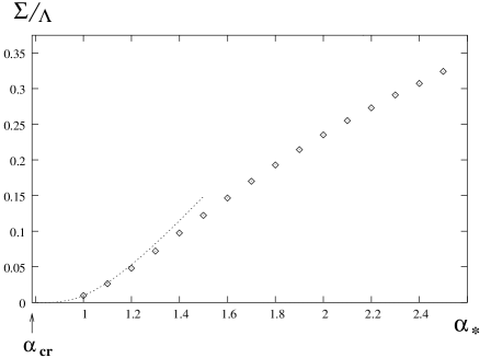
Figure 1: Numerical solutions for $\Sigma$, for several values of $\alpha_{*}$ (indicated by $\Diamond$). By way of comparison, we show, as the dotted curve, the solution (13) with $c=4.0$ derived from a fit to the results in the interval $0.89\leq\alpha_{*}\leq 1.0$. See text for further discussion.

Another quantity of interest is the pseudoscalar decay constant $f_{P}$, the $N_{f}$-flavor generalization of the pion decay constant. For $N_{f}=2$ QCD this is defined as $\langle 0|J^{j}_{\mu}|\pi^{k}(q)\rangle=if_{\pi}q_{\mu}\delta^{jk}$ where $1\leq j,k\leq 3$ are SU(2) isospin indices. Here, we use a generalization of this definition, with the symbol $f_{\pi}$ replaced by $f_{P}$ and the SU($N_{f}$) isospin indices in the range $1\leq j,k\leq N_{f}^{2}-1$. In QCD, one rough measure of the dynamical (constituent) quark mass is $\Sigma\simeq M_{N}/N_{c}\simeq 313$ MeV, where $M_{N}$ is the nucleon mass. An alternate definition sets $\Sigma\simeq M_{\rho}/2$; this would yield a somewhat larger value. Here we use the estimate $\Sigma\simeq 330$ MeV. Using the measured value $f_{\pi}\simeq 92.4\pm 0.3$ MeV pdg , one thus has

$$\bigg{(}\frac{\Sigma}{f_{\pi}}\bigg{)}_{QCD}\simeq 3.6\ .$$ (14)

An approximate relation connecting $\Sigma$ and $f_{P}$ is psrel (with $y\equiv k_{E}^{2}$)

$$f_{P}^{2}\,=\,\frac{N_{c}}{4\pi^{2}}\int_{0}^{\infty}y\,dy\,\frac{\Sigma^{2}(y)\,-\,\frac{y}{4}\,\frac{d}{dy}\left[\Sigma^{2}(y)\right]}{[y\ +\ \Sigma^{2}(y)\ ]^{2}}\ .$$ (15)

The integration is rendered finite by the softness of the dynamical mass $\Sigma(k_{E}^{2})$, which behaves for $k\gg\Sigma$ as

$$\Sigma(k_{E}^{2})\propto\Sigma\bigg{(}\frac{\Sigma}{k_{E}}\bigg{)}^{2-\gamma}$$ (16)

where $\gamma$ is the anomalous dimension of the bilinear operator $\bar{f}f$, having the value $\gamma\simeq 1$ in the walking regime and decreasing toward zero at very large energy scales $\mu>>\Lambda$ (since $\gamma$ is a power series in $\alpha$ and $\alpha\to 0$ in this limit due to the asymptotic freedom of the theory). Thus, the relation (15) suggests that for QCD

$$f_{\pi}^{2}\simeq\frac{N_{c}\Sigma^{2}}{4\pi^{2}}\ .$$ (17)

For $N_{c}=3$, this is $\Sigma/f_{\pi}\simeq 2\pi/\sqrt{3}\simeq 3.6$, which agrees, to within the theoretical uncertainties, with experiment. In QCD, with $\Lambda^{(2)}\simeq 400$ MeV, one has

$$\frac{f_{\pi}}{\Lambda^{(2)}_{QCD}}\simeq 0.25\ .$$ (18)

In Fig. 2 we show our results for $f_{P}$ calculated from substituting our solution for $\Sigma(k^{2})$ into eq. (15). In the walking limit, $f_{P}$ has been shown to satisfy a relation similar to eq. (13), i.e., it is exponentially smaller than the scale $\Lambda$. We display, as the dotted curve, the fit from Ref. mm for the walking interval $0.89\leq\alpha_{*}\leq 1.0$, given by eq. (13) with $c=1.5$. Our results show the change from this walking type of behavior as $\alpha_{*}$ increases above 1.2; as $\alpha_{*}$ increases from 1.0 to 2.5, $f_{P}/\Lambda$ increases substantially, from about $3\times 10^{-3}$ to about 0.08. This is similar to the factor by which we found that $\Sigma\Lambda$ increased as $\alpha_{*}$ increased through this interval.

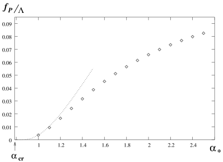
Figure 2: Values of $f_{P}$ calculated from eq. (15) for several values of $\alpha_{*}$ (indicated by $\Diamond$). For comparison, we show, as the dotted line, the analytic solution given by eq. (13) with $\Sigma$ replaced by $f_{P}$ and $c=1.5$ derived from a fit to the calculations for $0.89\leq\alpha_{*}\leq 2.5$. See text for further discussion.

The strong increase in $\Sigma/\Lambda$ and $f_{P}/\Lambda$ as $\alpha_{*}$ ascends from the value 0.89 near the walking limit to the value 2.5 deeper within the confinement phase is easily understood as reflecting the removal of the extreme exponential suppression evident in eq. (13) and its analogue for $f_{P}$ for $\alpha_{*}-\alpha_{cr}\to 0^{+}$. One does not expect such a dramatic change in the ratio $\Sigma/f_{P}$ over this interval, and this expectation is borne out by our calculations. In Fig. 3 we show the ratio of $\Sigma/f_{P}$, which increases gradually from about 2.6 to 3.9. The fact that we find a ratio comparable to the observed one in actual QCD, given by eq. (14), can be understood as a consequence of the property that much of the strong dependence on $N_{f}$ divides out in this ratio.

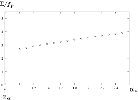
Figure 3: Plot of the ratio $\Sigma/f_{P}$ for $1\leq\alpha_{*}\leq 2.5$.

IV Calculation of Meson Masses via the Bethe-Salpeter Equation

IV.1 General Discussion

We denote the wavefunction for a hadron with a given flavor combination for the generalized $\pi$, $\rho$, etc. as follows. Define the flavor vector $f^{a}\equiv(f^{a1},...,f^{aN_{f}})$. Recall that in the confined phase the global symmetry ${\rm SU}(N_{f})_{L}\times{\rm SU}(N_{f})_{R}\times U(1)_{V}$ is broken spontaneously to ${\rm SU}(N_{f})_{V}\times{\rm U}(1)_{V}$. We drop the explicit subscript $V$ on ${\rm SU}(N_{f})_{V}$ henceforth. With regard to ${\rm SU}(N_{f})$, a $f\bar{f}$ meson with a given $J^{PC}$ (where $J$ denotes the spin, and $P$ and $C$ are the parity and charge conjugate eigenvalues) is described via the Clebsch-Gordan decomposition $N_{f}\times\bar{N}_{f}=1+Adj$, where 1 and $Adj$ denote the singlet and adjoint representations.

Let the generators of the group ${\rm SU}(N_{f})$ have the standard normalization ${\rm Tr}(T_{i}T_{j})=(1/2)\delta_{ij}$. Then the hadrons transforming according to the adjoint representation of ${\rm SU}(N_{f})$ are comprised of (i) the set of $N_{f}(N_{f}-1)$ states

$$h_{\Gamma;ij}=\frac{1}{\sqrt{N_{c}}}\sum_{a=1}^{N_{c}}\bar{f}_{a}\,\Gamma\,T_{ij}\,f^{a}$$ (19)

where $T_{ij}$ is the $N_{f}\times N_{f}$ matrix with a 1 in the $i$’th column and $j$’th row, with $1\leq i,j\leq N_{f}$, $i\neq j$, and $\Gamma$ specifies the type of particle (pseudoscalar, vector, axial-vector, scalar), and (ii) the $N_{f}-1$ states corresponds to the generators of the Cartan subalgebra of ${\rm SU}(N_{f})$ given by the traceless $N_{f}\times N_{f}$ matrices

$$T_{dk}=[2k(k+1)]^{-1/2}{\rm diag}(1,1,..,1,-k,0,..,0)$$ (20)

where there are $k$ 1’s and $1\leq k\leq N_{f}-1$. That is, $T_{d1}=(1/2){\rm diag}(1,-1,...,0)$, $T_{d2}=(2\sqrt{3})^{-1}{\rm diag}(1,1,-2,0,...,0)$, etc. Because of the ${\rm SU}(N_{f})$ flavor symmetry, it does not matter which of these $N_{f}^{2}-1$ hadrons with a given $\Gamma$ we use. We shall refer to these as the $N_{f}$-generalized $\rho$, $\omega$, etc. In particular, the spectrum of mesons includes a set of $N_{f}^{2}-1$ Nambu-Goldstone bosons (NGB’s) with $L=S=0$ and $J^{PC}=0^{-+}$, transforming according to the adjoint representation of ${\rm SU}(N_{f})$. The corresponding $0^{-+}$ singlet with respect to ${\rm SU}(N_{f})$, i.e., the generalized $\eta^{\prime}$, is not a Nambu-Goldstone boson because the corresponding U(1)_A symmetry is anomalous. Our analysis of meson masses is for the lowest-lying $f\bar{f}$ states. In future work one could also consider radial excitations, Regge recurrences, pure gluonic states (glueballs) and the general coupled situation in which glueballs and $f\bar{f}$ mesons of the same $J^{PC}$ mix.

In QCD, there are several (light-quark) $\bar{q}q$ mesons that are of interest here. For the reader’s convenience, we list these in Table 1. A notation for the various states in the case of general $N_{f}$ massless quarks is $S_{R}$, $P_{R}$, $V_{R}$, and $A_{R}$, standing for “scalar, pseudoscalar, vector, and axial-vector”, where the subscript $R$ denotes the representation - adjoint or singlet - under the SU($N_{f}$) flavor symmetry group. The experimental and theoretical situation concerning the $0^{++}$ isoscalar meson $f_{0}$ has been the subject of much discussion over the years; indeed, this state may involve mixing with $qq\bar{q}\bar{q}$ mesons schechter . Because of the complications in the analysis of this state, and the expected complications in a realistic analysis of its $N_{f}$-generalization, the SU($N_{f}$)-singlet $0^{++}$ meson, we do not attempt to treat this in our current study.

Table 1: Data on relevant $q\bar{q}$ mesons whose masses are compared with Bethe-Salpeter calculations. $n{}^{2S+1}\,L_{J}$ is standard spectroscopic notation, where $n$ denotes radial quantum number. The symbols adj. and sing. denote the adjoint and singlet representations of the SU(2)_V isospin flavor symmetry group. Masses are given in MeV, from pdg . The last column lists the mass divided by a typical hadronic scale, $f_{\pi}$.

$n{}^{2S+1}\,L_{J}$	$J^{PC}$	$R_{SU(2)_{V}}$	name	$M$	$M/f_{\pi}$
$1{}^{3}\,S_{1}$	$1^{--}$	adj.	$\rho$	$775.8\pm 0.5$	8.40
$1{}^{3}\,S_{1}$	$1^{--}$	sing.	$\omega$	$782.6\pm 0.1$	8.47
$1{}^{1}\,P_{1}$	$1^{+-}$	adj.	$b_{1}$	$1229.5\pm 3.2$	13.3
$1{}^{1}\,P_{1}$	$1^{+-}$	sing.	$h_{1}$	$1170\pm 20$	$12.7\pm 0.2$
$1{}^{3}\,P_{0}$	$0^{++}$	adj.	$a_{0}$	$984.7\pm 1.2$	10.7
$1{}^{3}\,P_{0}$	$0^{++}$	sing.	$f_{0}$	$\sim 600^{+600}_{-200}$	$6.5^{+6.5}_{-4.3}$
$1{}^{3}\,P_{1}$	$1^{++}$	adj.	$a_{1}$	$1230\pm 40$	$13.3\pm 0.4$
$1{}^{3}\,P_{1}$	$1^{++}$	sing.	$f_{1}$	$1281.8\pm 0.6$	13.9

As will be seen below, in the Bethe-Salpeter equation that we use to calculate the masses of the mesons, the flavor-dependent structure is simply a prefactor. Hence, the solutions of this equation have the property that, for a given radial quantum number and spectroscopic form ${}^{2S+1}\,L_{J}$, the SU($N_{f}$) flavor-singlet and flavor-adjoint mesons are degenerate:

$$M(n{}^{2S+1}\,L_{J};{\rm flav.\ adjoint})=M(n{}^{2S+1}\,L_{J};{\rm flav.\ singlet})$$ (21)

In view of this, we henceforth drop the subscript $R$ and simply write $V$ rather than $V_{flav.adj.}$ or $V_{flav.sing.}$, etc. Note that this is different from the prediction from SU($N_{f}$) flavor symmetry (with degenerate quarks and electroweak interactions turned off) that the members of a given representation of SU($N_{f}$) are degenerate. Experimentally, except for the pseudoscalar mesons, the light-quark isospin-adjoint and isospin-singlet $q\bar{q}$ mesons are nearly degenerate. The physical $\omega$ meson is very nearly a singlet under isospin SU(2), so a measure of this predicted degeneracy for the ground state $1^{--}$ mesons is $(M_{\omega}-M_{\rho})/[(1/2)((M_{\omega}+M_{\rho})]=0.87\times 10^{-2}$, quite small. Similarly, $(M_{f_{1}}-M_{a_{1}})/[(1/2)((M_{f_{1}}+M_{a_{1}})]=0.04\pm 0.03$ and $(M_{h_{1}}-M_{b_{1}})/[(1/2)((M_{h_{1}}+M_{b_{1}})]=-0.05\pm 0.02$. So for these states the prediction from our Bethe-Salpeter technique for the special case $N_{f}=2$ massless quarks is in agreement with the data for light-quark mesons in QCD.

The situation with the $0^{-+}$ mesons is quite different. Since the SU($N_{f}$) flavor-singlet mesons are not NGB’s, owing to the anomalous nature of the U(1)_A symmetry, they are split by a large mass difference from the flavor-adjoint NGB’s. In this case, as noted above, the semi-perturbative Bethe-Salpeter analysis does not contain the relevant physics involving instantons, and hence its prediction is far from reality. For this reason we do not consider the flavor-singlet $0^{-+}$ mesons here. As regards the flavor-adjoint $0^{-+}$ mesons, since we assume massless fermions and have turned off electroweak interactions, the mass $M_{P}$ of the flavor-adjoint pseudoscalar mesons is exactly zero in our calculations.

The pion decay constant $f_{\pi}$ provides a convenient mass scale with which to normalize the hadron masses. For comparison with our results calculated in the case of general larger $N_{f}$, we list in Table 1 the masses of the $q\bar{q}$ mesons divided by $f_{\pi}$. For later use we also record the ratio

$$\frac{M_{a_{1}}}{M_{\rho}}=1.59\pm 0.05\ .$$ (22)

This is slightly larger than the prediction $M_{a_{1}}/M_{\rho}=\sqrt{2}\simeq 1.414$ from a combination of vector meson dominance and spectral function sum rules wein . Also,

$$\frac{M_{a_{0}}}{M_{\rho}}=1.27\ .$$ (23)

An interesting result of the calculations of meson masses in the walking limit in Ref. mm was that the ratios of these masses to $f_{P}$ are rather constant. Specifically, it was found that in for $0.89\leq\alpha_{*}\leq 1.0$,

$$\frac{M_{V}}{f_{P}}\simeq 11\ ,$$ (24)

$$\frac{M_{A}}{f_{P}}\simeq 11.5\ ,$$ (25)

and

$$\frac{M_{S}}{f_{P}}\simeq 4.1\ ,$$ (26)

so that

$$\frac{M_{A}}{M_{V}}=1.04$$ (27)

and

$$\frac{M_{S}}{M_{V}}=0.36\ ,$$ (28)

where the theoretical uncertainty is several per cent. These ratios may be compared with the values in regular QCD which, as far as the light-meson spectrum is concerned, are close to the values that they would have in the $N_{f}=2$ chiral limit (with the understanding that the pion masses would actually vanish in this limit if electroweak interactions are turned off, as assumed here). For the purpose of this comparison, we do not try to use the inferred chiral-limit value of $f_{\pi}$ fpi , since to be consistent we would have to do the same for the mesons themselves. For the comparison between the extreme walking limit (WL) and QCD, we have

$$\frac{(M_{V}/f_{P})_{WL}}{(M_{\rho}/f_{\pi})}\simeq 1.3$$ (29)

$$\frac{(M_{A}/f_{P})_{WL}}{(M_{a_{1}}/f_{\pi})}\simeq 0.86\ ,$$ (30)

and

$$\frac{(M_{S}/f_{P})_{WL}}{(M_{a_{0}}/f_{\pi})}\simeq 0.38\ .$$ (31)

A major output of the present work is the elucidation of how, as $N_{f}$ decreases and $\alpha_{*}$ increases, the ratios of meson masses to $f_{P}$ begin to shift toward their QCD values.

V Calculations

Next, we describe the details of our solution of the Bethe-Salpeter equation and the resulting masses of $f\bar{f}$ mesons.

V.1 Bethe-Salpeter amplitudes

We introduce the Bethe-Salpeter amplitudes $\chi$ for the scalar ($S$), pseudoscalar ($P$), vector ($V$), and axial-vector ($A$) bound states of quark and anti-quark as follows :

$$\langle 0|T\psi_{\alpha fi}(x_{+})\ \bar{\psi}_{\beta}^{f^{\prime}j}(x_{-})\ |S_{a}(q)\rangle$$ (32)

$$=\sqrt{2}\,\delta_{i}^{j}(T_{a})_{f}^{f^{\prime}}\,e^{-iq\cdot X}\int\frac{d^{4}p}{(2\pi)^{4}}e^{-ip\cdot r} [\chi_{(S)}(p;q)]_{\alpha\beta}$$ ,

$$\langle 0|\ T\ \psi_{\alpha fi}(x_{+})\ \bar{\psi}_{\beta}^{f^{\prime}j}(x_{-})\ |P_{a}(q)\rangle$$ (33)

$$=\sqrt{2}\,\delta_{i}^{j}(T_{a})_{f}^{f^{\prime}}\,e^{-iq\cdot X}\int\frac{d^{4}p}{(2\pi)^{4}}e^{-ip\cdot r} [\chi_{(P)}(p;q)]_{\alpha\beta}$$ ,

$$\langle 0|\ T\ \psi_{\alpha fi}(x_{+})\ \bar{\psi}_{\beta}^{f^{\prime}j}(x_{-})\ |V_{a}(q,\epsilon)\rangle$$ (34)

$$=\sqrt{2}\,\delta_{i}^{j}(T_{a})_{f}^{f^{\prime}}\,e^{-iq\cdot X}\int\frac{d^{4}p}{(2\pi)^{4}}e^{-ip\cdot r} [\chi_{(V)}(p;q,\epsilon)]_{\alpha\beta}$$ ,

$$\langle 0|\ T\ \psi_{\alpha fi}(x_{+})\ \bar{\psi}_{\beta}^{f^{\prime}j}(x_{-})\ |A_{a}(q,\epsilon)\rangle$$ (35)

$$=\sqrt{2}\,\delta_{i}^{j}(T_{a})_{f}^{f^{\prime}}\,e^{-iq\cdot X}\int\frac{d^{4}p}{(2\pi)^{4}}e^{-ip\cdot r} [\chi_{(A)}(p;q,\epsilon)]_{\alpha\beta}$$ ,

where $x_{\pm}=X\pm r/2$, and ($\alpha$, $\beta$), ($f$, $f^{\prime}$), and ($i$, $j$) denote the spinor, flavor, and color indices, respectively. $\lambda_{a}$ represents flavor structure of the bound states. In the case of flavor-adjoint bound states, $T_{a}$ is the generator of $\mbox{SU}(N_{f})$, while in the case of flavor singlet bound states, $(T_{a})_{f}^{f^{\prime}}$ is the identity 1.

We expand the BS amplitude $\chi$ in terms of the bispinor bases $\Gamma^{i}$ and the invariant amplitudes $\chi^{(i)}$ as follows :

$$\left[\chi_{(S,P)}(p;q)\right]_{\alpha\beta}=\ \sum_{i=1}^{4}\left[\Gamma^{i}_{(S,P)}(p;q)\right]_{\alpha\beta}\chi_{(S,P)}^{(i)}(p;q),$$ (36)

$$\left[\chi_{(V,A)}(p;q,\epsilon)\right]_{\alpha\beta}=\ \sum_{i=1}^{8}\left[\Gamma^{i}_{(V,A)}(p;q,\epsilon)\right]_{\alpha\beta}\chi_{(V,A)}^{(i)}(p;q).$$ (37)

The bispinor bases can be determined from the spin, parity, and charge conjugation properties of the bound states. The explicit forms of $\Gamma_{(S)}^{i}$, $\Gamma_{(P)}^{i}$, $\Gamma_{(V)}^{i}$, and $\Gamma_{(A)}^{i}$ are summarized in Appendix A.

We take the rest frame of the bound state as a frame of reference:

$$q^{\mu}=(M_{B},0,0,0),$$ (38)

where $M_{B}$ represents the bound state mass, i.e., $M_{S},\ M_{P},\ M_{V}$ and $M_{A}$ for scalar, pseudoscalar, vector and axial-vector meson masses, respectively. After a Wick rotation, we parametrize $p^{\mu}$ by the real variables $u$ and $x$ as

$$p\cdot q=iM_{B}u\ ,\ p^{2}=-u^{2}-x^{2}.$$ (39)

Consequently, the invariant amplitudes $\chi^{(i)}$ can be expressed as functions of the variables $u$ and $x$:

$$\chi^{(i)}_{(S,P,V,A)}=\chi^{(i)}_{(S,P,V,A)}(u,x).$$ (40)

From the charge conjugation properties for the BS amplitude $\chi$ and the bispinor bases defined in Appendix A, the invariant amplitudes $\chi^{(i)}(u,x)$ are shown to satisfy the following relation:

$$\chi^{(i)}_{(S,P,V,A)}(u,x)=\chi^{(i)}_{(S,P,V,A)}(-u,x)\ .$$ (41)

V.2 Homogeneous Bethe-Salpeter equation

The homogeneous Bethe-Salpeter (HBS) equation is the self-consistent equation for the Bethe-Salpeter amplitude, and it is expressed as (see Fig. 4)

Figure 4: A graphical representation of the HBS equation in the (improved) ladder approximation

$$T\chi=K\chi\ .$$ (42)

The kinetic part $T$ is given by

$$T(p;q)=S_{f}^{-1}(p+q/2)\otimes S_{f}^{-1}(p-q/2)\ ,$$ (43)

where the BS kernel $K$ in the improved ladder approximation is expressed as

$$K(p;k)\ =\ C_{2f}\frac{4\pi\alpha(p,k)}{(p-k)^{2}}\left(g_{\mu\nu}-\frac{(p-k)_{\mu}(p-k)_{\nu}}{(p-k)^{2}}\right)\gamma^{\mu}\otimes\gamma^{\nu}.$$ (44)

In the above expressions we used the tensor product notation

$$(A\otimes B)\,\chi=A\,\chi\,B\ ,$$ (45)

and the inner product notation

$$K\chi\ (p;q)=-i\int\frac{d^{4}k}{(2\pi)^{4}}\ K(p,k)\ \chi(k;q)\ .$$ (46)

It should be noted that the fermion propagators included in $T$ in eq. (43) have complex-valued arguments after the Wick rotation sdcomplex . The arguments of the mass functions appearing in the two legs of the Bethe-Salpeter amplitude are expressed as

$$-(p\pm q/2)^{2}=u^{2}+x^{2}-\left(\frac{M_{B}}{2}\right)^{2}\mp iuM_{B}.$$ (47)

In general, it is difficult to obtain mass functions for complex arguments by solving the Schwinger-Dyson equation in the complex plane, especially because of the analytic structure of the running coupling in the complex momentum plane. However, in the case of large $N_{f}$ QCD, the analyticity of the two-loop running coupling constant Gardi makes it possible to solve for the mass function in the complex plane. This leads to the following approximation, in accordance with eq. (12) mm :

$${\rm Re}\left[\alpha(Xe^{i2\theta})\right] = \alpha_{\ast}\ \theta(\Lambda^{2}-X),$$ (48)

$${\rm Im}\left[\alpha(Xe^{i2\theta})\right] = 0.$$ (49)

where no confusion should result from the use of the symbol $\theta$ on the right-hand side of eq. (48) as the step function. .

V.3 Numerical results

We next present the results of the numerical calculations for the masses of the mesons. We solve the homogeneous Bethe-Salpeter equation as an eigenvalue problem, namely, the Bethe-Salpeter amplitude as an eigenfunction and the mass of a bound state as an eigenvalue, denoted generically as $M_{B}$. Because the eigenvalue $M_{B}$ appears nonlinearly in the equation, we use so-called fictitious eigenvalue method HY to obtain the value of $M_{B}$. For details of numerical method to solve HBS equation, see Ref. mm . In Fig. 5, we show the values of meson masses divided by $\Lambda$ calculated from the Schwinger-Dyson and Bethe-Salpeter equations in the range $0.9\leq\alpha_{*}\leq 2.5$. In Fig. 6 we plot the values of $M_{B}/f_{P}$ in the range of $0.9\leq\alpha_{*}\leq 2.5$. In Fig. 7, we plot the meson mass ratios $M_{A}/M_{V}$ and $M_{S}/M_{V}$ in the range of $0.9\leq\alpha_{*}\leq 2.5$.

Figure 5: Values of meson masses divided by $\Lambda$ calculated from the Schwinger-Dyson and Bethe-Salpeter equations.

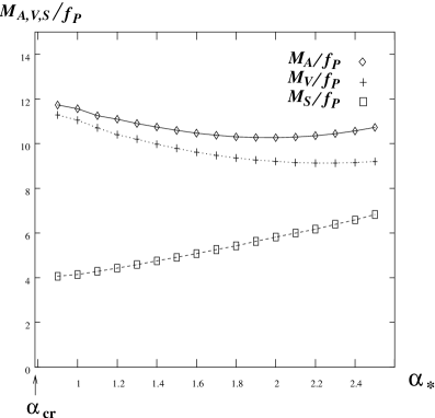
Figure 6: Values of meson masses divided by $F_{P}$ calculated from the Schwinger-Dyson and Bethe-Salpeter equations.

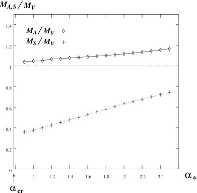
Figure 7: Ratios of meson masses calculated from the Schwinger-Dyson and Bethe-Salpeter equations.

Our calculations yield a number of interesting results. We summarize these for the changes in these meson masses as $\alpha_{*}$ increases from 0.9 to 2.5 as follows.

1. The ratios of the meson masses divided by $\Lambda$ increase dramatically, by factors of order $10^{2}$, approaching values of order unity at $\alpha_{*}=2.5$. This amounts to the removal of the exponential suppression of these masses which had described the walking limit at the boundary of the non-Abelian phase, as one moves away from this limit into the interior of the confined phase.

2. $M_{S}/f_{P}$ increases monotonically from about 4 to 7, thereby approaching to within about 35 % of the value 10.7 in QCD for $M_{a_{0}}/f_{\pi}$.

3. $M_{V}/f_{P}$ decreases from about 11 to 9, rather close to the value 8.5 for $M_{\rho}/f_{\pi}$ and $M_{\omega}/f_{\pi}$ in QCD. As is evident from Fig. 6, this ratio $M_{V}/f_{P}$ is roughly constant in the upper end of the interval of $\alpha_{*}$ values that we study.

4. $M_{A}/f_{P}$ behaves non-monotonically, first decreasing from roughly 11.5 to 10, but then increasing to about 11, within about 20 % of the average of the values in QCD for the isospin-triplet and isospin-singlet axial-vector mesons, 13 for $M_{a_{1}}/f_{\pi}$ and 14 for $M_{f_{1}}/f_{\pi}$.

5. Thus, the ratios $M_{A}/M_{V}$ and $M_{S}/M_{V}$, which were found in Ref. mm to have the respective values 1.04 and 0.36 in the walking limit, both increase in the interval of $\alpha_{*}$ that we study, reaching about 1.17 and 0.74, respectively, at $\alpha_{*}=2.5$. For comparison, these ratios are approximately 1.6 and 1.3 in QCD (cf. eqs. (22) and (23)). Although the value of the ratio $M_{S}/M_{V}$ at $\alpha_{*}=2.5$ is farther from its QCD value than is the case with $M_{A}/M_{V}$, it is increasing somewhat more rapidly as a function of $\alpha_{*}$, consistent with eventually approaching the QCD value.

VI Conclusions

In this paper we have considered a vectorial SU($N_{c}$) gauge theory with $N_{f}$ massless fermions transforming according to the fundamental representation and have studied the shift in behavior from walking that occurs in the region near the boundary between the confinement phase and the non-Abelian Coulomb phase to the QCD-like behavior with a non-walking coupling. Specifically, we have used the Schwinger-Dyson and Bethe-Salpeter equations to calculate the dynamically induced fermion mass $\Sigma$, the spontaneous chiral symmetry breaking parameter $f_{P}$, and the masses of the lowest-lying $q\bar{q}$ vector, axial-vector, and flavor-adjoint scalar mesons. We have investigated how these change as one decreases $N_{f}$ below $N_{f,cr}$, or equivalently, increases $\alpha_{*}$ above $\alpha_{cr}$, to move away from the above-mentioned boundary into the interior of the confinement phase. Our results show the crossover between walking and non-walking behavior in a gauge theory.

There are a number of interesting topics for future research using the methods of this paper. It would be useful to construct a kernel for the Bethe-Salpeter equation that could include more of the relevant physics, including instantons effects. Work is underway on this. It would also be worthwhile to calculate the masses of radially excited mesons and mesons with internal orbital angular momenta $L\geq 2$, as well as glueballs and the mixing between glueballs and $\bar{q}q$ mesons. We anticipate that the results of these calculations would exhibit the same general properties that we have found with the ground-state $\bar{q}q$ mesons, but it would be interesting to confirm this expectation explicitly. Another project would be to connect our study of the region in $N_{f}$ where there is a crossover from walking to nonwalking behavior, to the region around $N_{f}=2$. However, when one moves this far away from the walking regime, one loses a simplifying features of our calculation, namely the fact that we do not have to use an infrared cutoff on $\alpha$. Given that lattice gauge theory methods provide an ab initio framework for calculating hadron masses, we hope that the lattice community will extend early efforts such as those of Ref. mawhinney and carry out a definitive study of hadron masses in QCD with an arbitrary number of flavors. It would be of considerable interest to compare the results of the lattice calculations with those obtained from solutions of Schwinger-Dyson and Bethe-Salpeter equations.

Appendix A Bispinor bases for scalar, pseudoscalar, vector, and axial-vector bound states

In this appendix we show the explicit forms of the bispinor bases for the scalar, pseudoscalar, vector, and axial-vector bound states. Here we use the notation $\hat{q}_{\mu}=q_{\mu}/M_{B}$ with $M_{B}$ being the mass of the bound states, and $[a,b,c]\equiv a[b,c]+b[c,a]+c[a,b]$.

Bispinor base for the scalar bound state ($J^{PC}=0^{++}$) is given by

$$\Gamma_{(S)}^{1} = {\bf 1},\ \ \Gamma_{(S)}^{2}=\hbox to0.0pt{\hbox to5.03125pt{\hfil/\hfil}\hss}p,\ \ \Gamma_{(S)}^{3}=\hbox to0.0pt{\hbox to5.55557pt{\hfil/\hfil}\hss}\hat{q}(p\cdot\hat{q}),$$

$$\Gamma_{(S)}^{4} = \frac{1}{2}\ [\hbox to0.0pt{\hbox to5.03125pt{\hfil/\hfil}\hss}p,\hbox to0.0pt{\hbox to5.55557pt{\hfil/\hfil}\hss}\hat{q}],$$ (50)

and that for the pseudoscalar bound state ($J^{PC}=0^{-+}$) is given by

$$\Gamma_{(P)}^{1} = \gamma_{5},\ \ \Gamma_{(P)}^{2}=\hbox to0.0pt{\hbox to5.03125pt{\hfil/\hfil}\hss}p\ (p\cdot\hat{q})\ \gamma_{5},\ \ \Gamma_{(P)}^{3}=\hbox to0.0pt{\hbox to5.55557pt{\hfil/\hfil}\hss}\hat{q}\ \gamma_{5},$$

$$\Gamma_{(P)}^{4} = \frac{1}{2}\ [\hbox to0.0pt{\hbox to5.03125pt{\hfil/\hfil}\hss}p,\hbox to0.0pt{\hbox to5.55557pt{\hfil/\hfil}\hss}\hat{q}]\ \gamma_{5}\ .$$ (51)

Furthermore, for the vector bound state ($J^{PC}=1^{--}$) we use

$$\Gamma_{(V)}^{1}=\hbox to0.0pt{\hbox to5.00002pt{\hfil$\epsilon$\hfil}\hss}/,\ \ \Gamma_{(V)}^{2}=\frac{1}{2}[\hbox to0.0pt{\hbox to5.00002pt{\hfil$\epsilon$\hfil}\hss}/,\hbox to0.0pt{\hbox to5.03125pt{\hfil/\hfil}\hss}p](p\cdot\hat{q}),\ \ \Gamma_{(V)}^{3}=\frac{1}{2}[\hbox to0.0pt{\hbox to5.00002pt{\hfil$\epsilon$\hfil}\hss}/,\hbox to0.0pt{\hbox to5.55557pt{\hfil/\hfil}\hss}\hat{q}],$$

$$\Gamma_{(V)}^{4}=\frac{1}{3!}[\hbox to0.0pt{\hbox to5.00002pt{\hfil$\epsilon$\hfil}\hss}/,\hbox to0.0pt{\hbox to5.03125pt{\hfil/\hfil}\hss}p,\hbox to0.0pt{\hbox to5.55557pt{\hfil/\hfil}\hss}\hat{q}],\Gamma_{(V)}^{5}=(\epsilon\cdot p),\ \ \Gamma_{(V)}^{6}=\hbox to0.0pt{\hbox to5.03125pt{\hfil/\hfil}\hss}p(\epsilon\cdot p),$$

$$\Gamma_{(V)}^{7}=\hbox to0.0pt{\hbox to5.55557pt{\hfil/\hfil}\hss}\hat{q}(p\cdot\hat{q})(\epsilon\cdot p),\ \ \Gamma_{(V)}^{8}=\frac{1}{2}[\hbox to0.0pt{\hbox to5.03125pt{\hfil/\hfil}\hss}p,\hbox to0.0pt{\hbox to5.55557pt{\hfil/\hfil}\hss}\hat{q}](\epsilon\cdot p),$$ (52)

and for the axial-vector bound state ($J^{PC}=1^{++}$)

$$\Gamma_{(A)}^{1}=\hbox to0.0pt{\hbox to5.00002pt{\hfil$\epsilon$\hfil}\hss}/\ \gamma_{5},\ \ \ \Gamma_{(A)}^{2}=\frac{1}{2}[\hbox to0.0pt{\hbox to5.00002pt{\hfil$\epsilon$\hfil}\hss}/,\hbox to0.0pt{\hbox to5.03125pt{\hfil/\hfil}\hss}p]\gamma_{5},\ \ \ \Gamma_{(A)}^{3}=\frac{1}{2}[\hbox to0.0pt{\hbox to5.00002pt{\hfil$\epsilon$\hfil}\hss}/,\hbox to0.0pt{\hbox to5.55557pt{\hfil/\hfil}\hss}\hat{q}]\ (p\cdot\hat{q})\ \gamma_{5},$$

$$\Gamma_{(A)}^{4}=\frac{1}{3!}[\hbox to0.0pt{\hbox to5.00002pt{\hfil$\epsilon$\hfil}\hss}/,\hbox to0.0pt{\hbox to5.03125pt{\hfil/\hfil}\hss}p,\hbox to0.0pt{\hbox to5.55557pt{\hfil/\hfil}\hss}\hat{q}]\ \gamma_{5},\ \ \ \Gamma_{(A)}^{5}=(\epsilon\cdot p)\ (p\cdot\hat{q})\ \gamma_{5},$$

$$\Gamma_{(A)}^{6}=\hbox to0.0pt{\hbox to5.03125pt{\hfil/\hfil}\hss}p(\epsilon\cdot p)\ \gamma_{5},\ \ \Gamma_{(A)}^{7}=\hbox to0.0pt{\hbox to5.55557pt{\hfil/\hfil}\hss}\hat{q}\ (\epsilon\cdot p)\ (p\cdot\hat{q})\ \gamma_{5},$$

$$\Gamma_{(A)}^{8}=\frac{1}{2}[\hbox to0.0pt{\hbox to5.03125pt{\hfil/\hfil}\hss}p,\hbox to0.0pt{\hbox to5.55557pt{\hfil/\hfil}\hss}\hat{q}](\epsilon\cdot p)\ (p\cdot\hat{q})\ \gamma_{5}.$$ (53)

References

- (1) An early paper on the phase structure of vectorial gauge theories is T. Banks and A. Zaks, Nucl. Phys. B 196, 189 (1982).
- (2) B. Holdom, Phys. Lett. B 150, 301 (1985).
- (3) K. Yamawaki, M. Bando, and K. Matumoto, Phys. Rev. Lett. 56, 1335 (1986).
- (4) T. Appelquist, D. Karabali, and L. C. R. Wijewardhana, Phys. Rev. Lett. 57, 957 (1986); T. Appelquist and L. C. R. Wijewardhana, Phys. Rev. D 35, 774 (1987); Phys. Rev. D 36, 568 (1987).
- (5) T. Appelquist, J. Terning, and L. C. R. Wijewardhana, Phys. Rev. Lett. 77, 1214 (1996).
- (6) V. Miransky and K. Yamawaki, Phys. Rev. D 55, 5051 (1997); it ibid. 56, E 3768 (1997). See also V. Miransky and P. Fomin, Sov. J. Part. Nucl. 16, 203 (1985).
- (7) T. Appelquist, A. Ratnaweera, J. Terning, and L. C. R. Wijewardhana, Phys. Rev. D 58, 105017 (1998).
- (8) M. Harada, M. Kurachi, and K. Yamawaki, Phys. Rev. D 68, 076001 (2003).
- (9) See, e.g., F. Close, Introduction to Quarks and Partons (Academic, New York, 1979).
- (10) A. Chodos, R. Jaffe, K. Johnson, C. Thorn, and V. Weisskopf, Phys. Rev. D 9, 3471 (1974); T. DeGrand, R. Jaffe, K. Johnson, and J. Kiskis, Phys. Rev. D 12, 2060 (1975).
- (11) T. Degrand and R. Jaffe, Annals Phys. 100, 425 (1976).
- (12) For recent reviews, see Lattice 2005, Dublin; http://www.maths.tcd.ie/lat05; Lattice 2004, Fermilab, http:/lqcd.fnal.gov/lattice04; and earlier lattice field theory symposia.
- (13) E. Salpeter and H. Bethe, Phys. Rev. 84, 1232 (1951).
- (14) For an early review, see N. Nakanishi, Prog. Theor. Phys. Suppl. 43, 1 (1969).
- (15) T. Maskawa and H. Nakajima, Prog. Theor. Phys. 52, 1326 (1974);
- (16) R. Fukuda and T. Kugo, Nucl. Phys. B 117, 250 (1974); T. Kugo, Phys. Lett. B 76, 625 (1978).
- (17) K. Lane, Phys. Rev. D 10, 2605 (1974).
- (18) K. Higashijima, Phys. Rev. D 29, 1228 (1984).
- (19) T. Appelquist, K. Lane, and U. Mahanta, Phys. Rev. Lett. 61, 1553 (1988); T. Appelquist, U. Mahanta, D. Nash, and L.C.R. Wijewardhana, Phys. Rev. D 43, 646 (1991); U. Mahanta, Phys. Rev. D 45, 1405 (1992).
- (20) T. Kugo, in Proc. of 1991 Nagoya Spring School on Dynamical Symmetry Breaking, Nakatsugawa, Japan, 1991, ed. K. Yamawaki (World Scientific, Singapore, 1992).
- (21) V. Miransky, Dynamical Symmetry Breaking in Quantum Field Theories (World Scientific, Singapore, 1993).
- (22) M. Harada and Y. Yoshida, Phys. Rev. D 53, 1482 (1996).
- (23) K.-I. Aoki, M. Bando, T. Kugo, M. Mitchard, and H. Nakatani, Prog. Theor. Phys. 84, 683 (1990).
- (24) K.-I. Aoki, M. Bando, T. Kugo, and M. Mitchard, Prog. Theor. Phys. 85, 355 (1991).
- (25) K.-I. Aoki, T. Kugo, and M. Mitchard, Phys. Lett. B 266, 467 (1991).
- (26) P. Jain and H. Munczek, Phys. Rev. D 48, 5403 (1993).
- (27) C. J. Burden et al., Phys. Rev. C 55, 2649 (1997).
- (28) R. Alkofer and L. von Smekal, Phys. Rept. 353, 281 (2001).
- (29) P. Maris and C. D. Roberts, Int. J. Mod. Phys. E 12, 297 (2003).
- (30) M. Harada, M. Kurachi, and K. Yamawaki, Phys. Rev. D 70, 033009 (2004).
- (31) M. Harada, M. Kurachi, and K. Yamawaki, Prog. Theor. Phys. 115, 765 (2006) (hep-ph/0509193).
- (32) Here and below, when we mention non-integral values of , it is implicitly understood that physical values of are, of course, positive integers, and the non-integral values are defined via an analytic continuation away from these physical values.
- (33) D. Gross and F. Wilczek, Phys. Rev. Lett. 30, 1343 (1973); H. D. Politzer, Phys. Rev. lett. 30, 1346 (1973); G. ’t Hooft, unpublished.
- (34) W. Caswell, Phys. Rev. Lett. 33, 244 (1974); D. R. T. Jones, Nucl. Phys. B 75, 531 (1974).
- (35) The Casimir invariant of the representation is defined by , where and denote group and representation indices and sums over repeated indices are understood.
- (36) D. Caldi, Phys. Rev. Lett. 39, 121 (1977); C. Callan, R. Dashen, and D. Gross, Phys. Rev. D 17, 2717 (1978); T. Appelquist and S. Selipsky, Phys. Lett. B 400, 364 (1997).
- (37) Y. Iwasaki et al., Phys. Rev. Lett. 69, 21 (1992); Phys. Rev. D 69, 014507 (2004).
- (38) P. Damgaard, U. Heller, A. Krasnitz, and P. Olesen, Phys. Lett. B 400, 169 (1997).
- (39) R. Mawhinney, Nucl. Phys. B (Proc. Suppl.) 63A-C, 212 (1998); R. Mawhinney, Nucl. Phys. B (Proc. Suppl.) 83, 57 (2000).
- (40) It has been estimated gl85 that , where denotes the value of in the chiral limit . With , this gives MeV.
- (41) J. Gasser and H. Leutwyler, Nucl. Phys. B 250, 465 (1985). See also Ref. chipt .
- (42) J. Gasser and H. Leutwyler, Phys. Rept. C 87, 77 (1982); Nucl. Phys. B 250, 517 (1985); G. Colangelo, J. Gasser, and H. Leutwyler, Nucl. Phys. B 603, 125 (2001); M. Harada and K. Yamawaki, Phys. Rept. 381,1 (2004); U.-G. Meissner, hep-ph/0501009.
- (43) For a compendium of relevant data and references, see http://pdg.lbl.gov.
- (44) H. Pagels and S. Stokar, Phys. Rev. D 20, 2947 (1979).
- (45) D. Black, A. Fariborz, F. Sannino, and J. Schechter, Phys. Rev. D 59, 074026 (1999); A. Fariborz, R. Jora, and J. Schechter, hep-ph/0601216.
- (46) S. Weinberg, Phys. Rev. Lett. 18, 507 (1967).
- (47) The Schwinger-Dyson equation with variables in the complex plane was discussed by T. Kugo and Y. Yoshida, Soryushiron Kenkyu 91, B26 (1995). See also Ref. mm for more a detailed discussion.
- (48) E. Gardi and M. Karliner, Nucl. Phys. B 529, 383 (1998); E. Gardi, G. Grunberg and M. Karliner, JHEP 9807, 007 (1998).