Self-consistent variational approach to the minimal left-right symmetric model of electroweak interactions

Abstract

The problem of mass generation is addressed by a Gaussian variational method for the minimal left-right symmetric model of electroweak interactions. Without any scalar bidoublet, the Gaussian effective potential is shown to have a minimum for a broken symmetry vacuum with a finite expectation value for both the scalar Higgs doublets. The symmetry is broken by the fermionic coupling that destabilizes the symmetric vacuum, yielding a self consistent fermionic mass. In this framework a light Higgs is only compatible with the existence of a new high energy mass scale below 2 TeV.

I introduction

It has been recently suggestedsiringo ; brahmachari ; siringo2 that mass generation and the breaking of left-right symmetry can be described by a minimal left-right symmetric model with only two scalar doublets and no bidoublets. Several left-right symmetric extensions of the standard model have been developed by many authorspati ; mohapatra ; senjanovic2 ; senjanovic and are based on the gauge group $SU(2)_{L}\times SU(2)_{R}\times U(1)_{B-L}$. They have the remarkable merit of predicting the same low energy phenomenology of the standard modeltheorem , thus explaining the lack of symmetry of the electroweak interactions. However, most of those models also contain a scalar Higgs bidoublet and require the existence of ten physical Higgs particles at least. A minimal model with only two scalar doublets $\Phi_{L}$, $\Phi_{R}$ transforming as $(2,1,1)$ and $(1,2,1)$ respectively, would require the existence of just two physical Higgs particles and would be an appealing alternative provided that a stable vacuum with a non zero expectation value $v_{L}=\langle\Phi_{L}\rangle$ can be found. It has been pointed outsiringo2 ; senjanovic2 that without any bidoublet the effective potential has a minimum for $\langle\Phi_{R}\rangle=v_{R}\not=0$ and $\langle\Phi_{L}\rangle=v_{L}=0$ and the model would be useless as $v_{L}=v_{Fermi}$ gives the scale of all the known particle masses. In fact the insertion of a scalar bidoublet was the simplest way of shifting the minimum of the effective potential towards a small but finite $v_{L}$ value. In spite of that, the minimal model has gained some success and its prediction of a new intermediate physical mass scale $v_{R}$ has been already exploredalmeida showing that the new physics could appear at the TeV scale in the new electron-positron colliders.

In this paper we give a self-consistent solution to the open problemsiringo2 of a physical vacuum for the minimal model: we show that the inclusion of quantum fluctuations yields a stable vacuum with $v_{L}\not=0$ even without any bidoublet, thus motivating and enforcing previous work on the modelbrahmachari ; almeida . The problem is addressed by a variational method, as we show that in the minimal model the minimum of the Gaussian Effective Potentialschiff ; rosen ; barnes ; kuti ; chang ; weinstein ; huang ; bardeen ; peskin ; stevenson is shifted towards a small finite $v_{L}$ value by the coupling to fermions. The variational character of the calculation is important as it ensures that the $v_{L}=0$ vacuum is not stable even without any scalar bidoublet. Thus the coupling to fermions is no longer a mere way to generate the Dirac masses, but it becomes the source of symmetry breaking for the field $\Phi_{L}$ yielding a self consistent mass for the heavy top quark.

The paper is organized as follows: in section II an effective low-energy Lagrangian is recovered from the full left-right symmetric model; the vacuum stability of the effective model is studied in section III by a variational method for the effective potential; in section IV the effective potential is discussed together with its predictions for the mass spectra.

II effective low-energy model

The problem of a viable physical vacuum for the minimal model has been recently addressed by invoking the existence of a larger approximate global symmetry in addition to the discrete parity symmetrysiringo . The physical Higgs particle would emerge as the pseudo-Goldstone boson associated with the breaking of the global symmetry. In that scenario the fermionic one-loop contributions to the effective potential become relevant for determining the minimum of the effective potential and the mass scale $v_{L}$. It emerges that the zero-point fermionic energy destabilizes the $v_{L}=0$ vacuum in competition with the bosonic terms. The approximate global symmetry has the further merit of being accidentally respected by any quadratically divergent contribution to the Higgs potentialchacko , thus we expect that the global symmetry should survive in the low energy effective Lagrangian of the Higgs sector up to small symmetry breaking terms. Then we take the Higgs potential to be

$${\cal L_{H}} = \frac{1}{2}M_{B}^{2}\left(\Phi_{L}^{\dagger}\Phi_{L}+\Phi_{R}^{\dagger}\Phi_{R}\right)+$$ (1)

$$+ \frac{1}{4!}\lambda\left(\Phi_{L}^{\dagger}\Phi_{L}+\Phi_{R}^{\dagger}\Phi_{R}\right)^{2}+\frac{1}{2}\eta\>\Phi_{L}^{\dagger}\Phi_{L}\Phi_{R}^{\dagger}\Phi_{R}$$

where $\eta$ is a small parameter which breaks the global $SU(4)$ symmetry. At variance with soft symmetry breaking modelsbabu where the left-right symmetry is broken by insertion of different masses for left and right fields, our Higgs potential is assumed to be fully symmetric. Thus the present model provides a truly spontaneous symmetry breaking mechanism.

In unitarity gauge the doublets may be taken as $\Phi_{L,R}=(0,\phi_{L,R})$ where the scalar real components $\phi_{L,R}$ describe two physical neutral bosons. For $\eta>0$ and $M_{B}^{2}<0$ the potential has a minimum for $\phi_{L}=0$ and $\phi_{R}^{2}=v_{R}^{2}=-6M_{B}^{2}/\lambda$. We may set $\phi_{R}=v_{R}+h_{R}$ and write the new potential for the field $h_{R}$ as ${\cal L_{H}}={\cal L}_{L}+{\cal L}_{R}+{\cal L}_{int}$

$${\cal L}_{L}=\frac{1}{2}(\eta v_{R}^{2})\phi_{L}^{2}+\frac{1}{4!}\lambda\phi_{L}^{4}$$ (2)

$${\cal L}_{R}=\frac{1}{3!}(\lambda v_{R}^{2})h_{R}^{2}+\frac{1}{3!}(\lambda v_{R})h_{R}^{3}+\frac{1}{4!}\lambda h_{R}^{4}$$ (3)

$${\cal L}_{int}=\frac{1}{2}\left(\eta+\frac{\lambda}{3!}\right)\phi_{L}^{2}h_{R}^{2}+\left(\eta+\frac{\lambda}{3!}\right)v_{R}\phi_{L}^{2}h_{R}$$ (4)

Assuming that $\lambda\gg\eta$, the heavy Higgs field $h_{R}$ is decoupled and we can regard Eq.(2) as the effective low-energy Lagrangian for the field $\phi_{L}$. A natural cut-off $\Lambda\approx v_{R}$ comes from the requirement that the physical vacuum is stable around the broken symmetry point $\phi_{L}=0$, $\phi_{R}=v_{R}$. The full effective Lagrangian for the field $\phi_{L}$ is easily recovered by adding the kinetic terms and the coupling to fermions and gauge bosons. Provided that the vacuum expectation value $\langle\phi_{L}\rangle=v_{L}$ does not vanish, the model gives rise to the standard phenomenology with the gauge bosons acquiring masses at two different scales: a small mass scale $v_{L}$ for the standard model light bosons $W^{\pm}_{L}$, $Z$, and a larger mass scale $v_{R}$ for the heavy gauge bosons $W^{\pm}_{R}$, $Z^{\prime}$. The details of the symmetry breaking are dicussed in Ref.siringo where the standard model Lagrangian is recovered up to ${\cal O}(v_{L}^{2}/v_{R}^{2})$ corrections. Moreover, without any Higgs bidoublet, the charged bosons $W^{\pm}_{L}$ and $W^{\pm}_{R}$ are shown to be exactly decoupled. The heavy bosons are decoupled any way in the low energy domain where they hardly play any role if $v_{R}\gg v_{L}$.

Here our main concern is the shift of the vacuum expectation value of $\phi_{L}$ from the $\phi_{L}=0$ minimum of the potential ${\cal L}_{L}$ in Eq.(2). Thus we neglect the weak coupling to the gauge bosons and insert the coupling to Dirac fermion fields $\psi_{i}$siringo ; brahmachari ; weinberg

$${\cal L}_{f}=\sum_{i}q_{i}\bar{\psi}_{i}\psi_{i}\phi_{L}\phi_{R}$$ (5)

where the index $i$ runs over the different kinds of quarks and leptons. Since all the fermions but the top quark $\psi_{t}$ may be neglected for their small coupling constants, in the Euclidean formalism the full effective Lagrangian reads

$${\cal L}_{eff}=\frac{1}{2}(\partial_{\mu}\phi_{L})^{2}+\bar{\psi}_{t}(\hbox to0.0pt{/\hss}\partial+\alpha\phi_{L})\psi_{t}+\frac{1}{2}M^{2}\phi_{L}^{2}+\frac{1}{4!}\lambda\phi_{L}^{4}$$ (6)

where $M^{2}=\eta v_{R}^{2}>0$ and $\alpha=q_{t}v_{R}$.

A simple dimensional argument would suggest that the coupling constants $q_{i}$ scale like the inverse of some large energy $\Gamma$. Moreover, according to Eq.(6), the term $\alpha v_{L}$ is the mass of the top quark $m_{t}$ which is not too much smaller than $v_{L}$. Thus the adimensional coupling $\alpha$ is of order unity and $\Gamma$ turns out to be only slightly above $v_{R}$. One may wonder in that case whether the effective operator in Eq.(5) makes sense for the top quark. The problem has been addressed in Ref.brahmachari where it is shown that up to a renormalization of couplings no serious change occurs in mass spectra. Of course, in order to address this point further, some extra hypothesis would be required on the origin of the dimension-five operatorsiringo ; brahmachari ; weinberg in Eq.(5).

At tree level the effective Lagrangian Eq.(6) predicts a vanishing vacuum expectation value $v_{L}$ for the field $\phi_{L}$. However, in the next section we show that quantum fluctuations make the $v_{L}=0$ vacuum unstable towards a phenomenologically acceptable finite value.

III The Gaussian Effective Potential

It has been recently shownmarotta ; camarda that in three dimensions the scalar theory can be studied by the Gaussian Effective Potential (GEP)schiff ; rosen ; barnes ; kuti ; chang ; weinstein ; huang ; bardeen ; peskin ; stevenson0 ; stevenson yielding a very good interpolation of the experimental correlation lengths of superconductors. As those lengths are the inverse of the masses, we believe that the GEP method could give a reliable estimate of masses in four dimensions as well. The variational nature of this approximation makes it a more powerful tool than any perturbative approach, such as the one-loop effective potential (1LEP); in fact, it has been shown (see, for instance kuti ; chang ; stevenson0 ) that the GEP contains features which can not be obtained by calculations based on a finite order of loops, and it results well-defined even when the 1LEP becomes a complex (and so unphysical) quantity. Moreover the variational character of the GEP makes it reliable even in the strong coupling limit where the 1LEP makes no sense. In fact the effective Lagrangian Eq.(6) contains a Higgs self-interaction parameter $\lambda$ which is known to be of order unity or larger (siringo3 ), and any perturbative prediction on the vacuum stability would not be conclusive.

The GEP for the Lagrangian (6) has been studied by several authorsstevenson2 ; stancu2 and it is well known to be unbounded: the fermions encourage spontaneous symmetry breaking, and in four dimensions they destabilize the scalar theory in the limit of an infinite cut-off $\Lambda\to\infty$. However the effective theory has a natural cut-off $\Lambda\approx v_{R}$ and the inclusion of the fermionic couplings just gives rise to a spontaneous symmetry breaking for the field $\phi_{L}$ which acquires a small finite expectation value $v_{L}\ll v_{R}$.

As usual for the GEP methodstevenson ; stancu we take $\phi_{L}=\varphi+h_{L}$ where $\varphi$ is a constant shift and $h_{L}$ is the Higgs field. The Gaussian Lagrangian is taken as

$${\cal L}_{GEP}=\frac{1}{2}(\partial_{\mu}h_{L})^{2}+\frac{1}{2}\Omega^{2}h_{L}^{2}+\bar{\psi}_{t}(\hbox to0.0pt{/\hss}\partial+m)\psi_{t}$$ (7)

where $\Omega$ and $m$ are variational parameters for the masses. The GEP followsstevenson2

$$V(\varphi) = \left[I_{1}(\Omega)-4I_{1}(m)\right]+\frac{1}{2}M^{2}\varphi^{2}+\frac{1}{4!}\lambda\varphi^{4}+$$ (8)

$$+ \left[4m(m-\alpha\varphi)I_{0}(m)\right]+$$

$$+ \frac{1}{2}I_{0}(\Omega)\left[M^{2}-\Omega^{2}+\frac{1}{2}\lambda\varphi^{2}+\frac{1}{4}\lambda I_{0}(\Omega)\right]$$

where the integrals $I_{n}(x)$ are defined acording to

$$I_{1}(x)=\frac{1}{2}\int\frac{d^{4}p}{(2\pi)^{4}}\log(p^{2}+x^{2})$$ (9)

$$I_{0}(x)=2\frac{dI_{1}(x)}{dx^{2}}=\int\frac{d^{4}p}{(2\pi)^{4}}\frac{1}{p^{2}+x^{2}}$$ (10)

These diverging integrals are supposed to be regularized by the cut-off $p<\Lambda$, and their exact evaluation is trivial.

The minimum of $V(\varphi)$ is found by solving the system of coupled equations $\partial V/\partial\Omega=\partial V/\partial m=\partial V/\partial\varphi=0$, which reads

$$\Omega^{2} = M^{2}+\frac{1}{2}\lambda\varphi^{2}+\frac{1}{2}\lambda I_{0}(\Omega)$$ (11)

$$m = \alpha\varphi$$ (12)

$$4\alpha mI_{o}(m) = \varphi\left[M^{2}+\frac{1}{3!}\lambda\varphi^{2}+\frac{1}{2}\lambda I_{0}(\Omega)\right]$$ (13)

According to Eq.(12) the fermionic contribution to the effective potential is just the first order perturbative term evaluated at the self consistent mass $m=\alpha\varphi$.

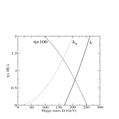
Figure 1: The free parameters $\lambda$ (solid line) and $\eta$ (dashed line) evaluated by Eqs.(14),(15) as functions of the Higgs mass $\Omega$ at the scale $v_{R}=1500$ GeV ($v_{R}/v_{L}\approx 6$). Since $\eta\ll\lambda$, the parameter $\eta$ has been rescaled by a factor 100. For comparison the standardstevenson GEP $\lambda_{S}$ is also reported (dotted line). The constraint $\lambda,\eta>0$ is only satisfied for $170<\Omega<253$ GeV for this choice of $v_{R}$.

We can show that for a broad range of the parameters the coupled equations have a broken symmetry solution for $\varphi=v_{L}\not=0$, thus yielding a finite mass for the fermion $m=\alpha v_{L}$. That can be easily seen by fixing $v_{L}$,$v_{R}$, $\Omega$ and $m$ at reasonable phenomenological values and by solving the coupled equations (11),(13) in order to get the free parameters $\lambda$, $\eta$. Since we want to recover the correct weak interaction phenomenology, the expectation value of $\phi_{L}$ must be set equal to the Fermi value $v_{L}=v_{Fermi}=247$ GeV. Moreover the Top quark mass is known to be $m_{t}=181$ GeV and then the coupling must be $\alpha=m_{t}/v_{L}=0.733$. By use of Eq.(11) we can write Eq.(13) as

$$\lambda=\frac{3}{v_{Fermi}^{2}}\left[\Omega^{2}-4\alpha^{2}I_{0}(m_{t})\right]$$ (14)

and this already provides a lower bound on the Higgs mass $\Omega$ as for $x\ll\Lambda$, $I_{0}(x)\approx\Lambda^{2}/(16\pi^{2})$ and the existence of a solution $\lambda>0$ requires that $\Omega>(\alpha\Lambda)/(2\pi)\approx 0.12\Lambda$. Thus the new high energy mass scale $v_{R}\approx\Lambda$ cannot be larger than ten times the Higgs mass $\Omega$. A comparison with the standardstevenson GEP relation $\lambda_{S}=3\Omega^{2}/v^{2}_{Fermi}$ shows that the parameter $\lambda$ is smaller in this minimal model, thus allowing for perturbative tretments up to a bit larger Higgs mass. However, as it can be seen from Fig. 1, the coupling costant $\lambda$ comes out to be of order of unity even for Higgs mass values $\Omega$ quite close to the experimental lower bound; this circumstance makes clear our choice of using the GEP variational method: the problem we are dealing with is a non perturbative one and an analysis based on perturbation theory is not reliable. Eq.(11) reads

$$\eta=\frac{1}{v_{R}^{2}}\left[\Omega^{2}-\frac{1}{2}\lambda\left(v^{2}_{Fermi}+I_{0}(\Omega)\right)\right]$$ (15)

The existence of a broken symmetry minimum in the potential ${\cal L_{H}}$ Eq.(1) requires that $\eta>0$, and since $\lambda=3\Omega^{2}/v^{2}_{Fermi}+const.$, according to Eq.(14) , we find an upper bound for the Higgs mass. At any fixed high energy scale $v_{R}\approx\Lambda$, the dependence on $\Omega$ of the parameters $\lambda$, $\eta$ is obtained by Eqs.(14),(15). We notice that, apart from a very narrow range at the lower bound of $\Omega$, the parameter $\eta$ is always small and $\eta\ll\lambda$ as it was required in order to decouple the heavier Higgs field $h_{R}$.

IV discussion

The existence of a broken symmetry vacuum with $v_{L}\not=0$ is a variational result: as the exact vacuum must have a smaller energy, we can conclude that the $v_{L}=0$ vacuum cannot be stable. Thus the choice of a variational method gives us more confidence on its prediction of a broken symmetry vacuum. Moreover the GEP gives rise to some bounds for the Higgs boson mass according to Eqs.(14),(15). The general behaviour is shown in Fig.1 for $v_{R}=1500$ GeV ($v_{R}/v_{L}\approx 6$) where the constraint $\lambda,\eta>0$ is only satisfied for $170<\Omega<253$ GeV.

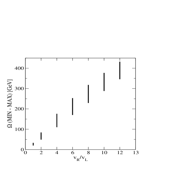
Figure 2: The allowed range for the Higgs mass $\Omega$ (vertical bars) are reported for several choices of the ratio $v_{R}/v_{L}$ between high energy and low energy mass scales ($v_{L}$ is fixed at the Fermi value $v_{Fermi}=247$ GeV).

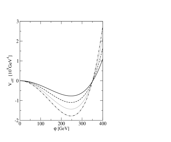
Figure 3: The Gaussian effective potential according to Eq.(8) for several choices of the Higgs mass and the high energy scale $v_{R}$. From the top: $\Omega=140$ GeV, $v_{R}=1000$ GeV (solid line); $\Omega=200$ GeV, $v_{R}=1500$ GeV (dashed line); $\Omega=260$ GeV, $v_{R}=2000$ GeV (dotted line); $\Omega=320$ GeV, $v_{R}=2500$ GeV (dot-dash). For each value of the shift $\varphi$ the GEP is evaluated by inserting in Eq.(8) the self-consistent masses $\Omega$, $m$ which solve the gap equations Eqs.(11),(12). The minimum point $\varphi=v_{L}$ does not change as it is fixed at the phenomenological value $v_{Fermi}=247$ GeV

.

The allowed range for the Higgs mass $\Omega$ is reported in Fig.2 for several choices of the high energy scale $v_{R}$. Assuming a rather light Higgs mass $\Omega\approx 200$ GeV, then the model is only consistent with an high energy scale $v_{R}\leq 1.7$ TeV. If for instance we take $v_{R}=1.5$ TeV, then the coupled linear equations (14), (15) have the solution $\lambda=0.554$ and $\eta=(M^{2}/v_{R}^{2})=8.6\cdot 10^{-3}$. In this scenario the search for new physics at the TeV scale could reveal the existence of the heavy Higgs field $h_{R}$ and the new heavy gauge bosons $W^{\pm}_{R}$ and $Z^{\prime}$, whose massessiringo would be larger by a factor $v_{R}/v_{L}\approx 6$ compared to their light partners. However, according to Fig.2, a larger Higgs mass would be compatible with a larger high energy scale, and a quite heavy Higgs at the TeV scale would require a large $v_{R}\approx 10$ TeV which in turn would push any chance to reveal the new physics towards higher energies. The effective potential Eq.(8) is reported in Fig.3 for average Higgs masses at different high energy scales $v_{R}$. For each value of the shift $\varphi$ the GEP is evaluated by inserting in Eq.(8) the self-consistent masses $\Omega$, $m$ which solve the gap equations Eqs.(11),(12). The minimum point $\varphi=v_{L}$ does not change as it is fixed at the phenomenological value $v_{Fermi}=247$ GeV by solution of the equations Eqs.(14), (15) for the parameters $\lambda$, $\eta$. Of course the curvature does change as the Higgs mass $\Omega$ does.

This simple variational study shows that the minimal left-right symmetric model, with only two Higgs doublets and no bidoublets could give a satisfactory description of the known phenomenology provided that quantum fluctuations are included. The model predicts the existence of a high energy mass scale $v_{R}$ which is not larger than ten times the Higgs mass. At the new energy scale the three right handed partners of the weak bosons should come out in experiments together with the second heavier higgs boson $h_{R}$. The model does not require the existence of other particles, and its predictions on masses could be tested in the new electron-positron colliders.

In summary we have shown that inclusion of the fermionic coupling is enough for destabilizing the $v_{L}=0$ vacuum of the minimal left-right symmetric model, thus yielding a small finite low energy scale $v_{L}\ll v_{R}$.

The genuine variational nature of the GEP method ensures that the instability of the $v_{L}=0$ vacuum is not a mere artifact introduced by the approximation, but a property of the model; furthermore the method allows for reliable predictions even in the strong coupling (heavy Higgs) regime, where any perturbative treatment (e.g. 1LEP) would not be valid. Thus even without any bidoublet, the minimal model is shown to be a viable framework for explaining the breaking of left-right symmetry in electroweak interactions.

References

- (1) F. Siringo, Eur. Phys. J. C 32, 555 (2004); hep-ph/0307320.
- (2) B. Brahmachari, E. Ma, U. Sarkar, Phys. Rev. Lett. 91, 011801 (2003).
- (3) F. Siringo, Phys. Rev. Lett. 92, 119101 (2004).
- (4) J.C. Pati and A. Salam, Phys.Rev. D10, 275 (1974).
- (5) R.N. Mohapatra and J.C. Pati, Phys.Rev.D 11, 566 (1975).
- (6) G. Senjanovic and R.N. Mohapatra, Phys.Rev.D 12, 1502 (1975).
- (7) G. Senjanovic, Nucl.Phys.B 153, 334 (1979).
- (8) That left-right symmetric theories predict the standard model phenomenology has been shown on very general grounds by Senjanovicsenjanovic who employed the method of Georgi and Weinberggeorgi2 .
- (9) H. Georgi and S. Weinberg, Phys.Rev.D 17, 275 (1978).
- (10) F.M.L. Almeida Jr., Y.A. Coutinho, J.A. Martins Simões, J. Ponciano, A.J. Ramalho, S. Wulck, M.A.B. Vale, Eur. Phys. J. C 38, 115 (2004).
- (11) L.I. Schiff, Phys. Rev. 130, 458 (1963).
- (12) G. Rosen, Phys. Rev. 173, 1632 (1968).
- (13) T. Barnes and G. I. Ghandour, Phys. Rev. D 22 , 924 (1980).
- (14) J. Kuti (unpublished), as discussed in J. M. Cornwall, R. Jackiw and E. Tomboulis, Phys. Rev. D 10, 2428 (1974).
- (15) J. Chang, Phys. Rev D 12, 1071 (1975); Phys. Rep. 23C, 301 (1975); Phys. Rev. D 13, 2778 (1976).
- (16) M. Weinstein, S. Drell, and S. Yankielowicz, Phys. Rev. D 14, 487 (1976).
- (17) K. Huang and D. R. Stump, Phys. Rev. D 14, 223 (1976).
- (18) W. A. Bardeen and M. Moshe, Phys. Rev. D 28, 1372 (1983).
- (19) M. Peskin, Ann. of Phys. 113, 122 (1978).
- (20) P. M. Stevenson, Phys. Rev. D 30, 1712 (1984).
- (21) P.M. Stevenson, Phys. Rev. D 32, 1389 (1985).
- (22) Z. Chacko, H.-S. Goh, and R. Harnik, SLAC-PUB-11595, hep-php/0512088.
- (23) K. S. Babu, R. N. Mohapatra, Phys. Rev. D 41, 1286 (1990).
- (24) S. Weinberg, Phys. Rev. Lett. 43, 1566 (1979).
- (25) L. Marotta, M. Camarda, G.G.N. Angilella and F. Siringo, Phys. Rev. B 73, 104517 (2006).
- (26) M. Camarda, G.G.N. Angilella, R. Pucci, F. Siringo, Eur. Phys. J. B 33, 273 (2003).
- (27) F. Siringo, Europhys. Lett. 59, 820 (2002); Phys. Rev. D 62, 116009 (2000).
- (28) P.M. Stevenson, G.A. Hajj, J.F. Reed, Phys. Rev. D 34, 3117 (1986).
- (29) I. Stancu, Phys. Rev. D 43, 1283 (1991).
- (30) I. Stancu, P.M. Stevenson, Phys. Rev. D 42, 2710 (1990).