Power Spectrum of the Density Perturbations From Smooth Hybrid New Inflation Model

Abstract

We numerically investigate density perturbations generated in the smooth hybrid new inflation model, a kind of double inflation model that is designed to reproduce the running spectral index suggested by the WMAP results. We confirm that this model provides the running spectral index within 1$\sigma$ range of the three year WMAP result. In addition, we find a sharp and strong peak on the spectrum of primordial curvature perturbation at small scales. This originates from amplification of fluctuation in the first inflaton fields due to parametric resonance, which takes place in the oscillatory phase between two inflationary regime. Formation probability of primordial black holes (PBHs) is discussed as a consequence of such peak.

I Introduction

The observation of Wilkinson Microwave Anisotropy Probe (WMAP) has successfully determined the cosmological parameters and nature of density fluctuations with high precision. The WMAP result is quite consistent with the prediction of the inflationary cosmology, i.e., the flat universe with almost scale-invariant adiabatic density fluctuation. If one take a closer look at the shape of the power spectrum of the density fluctuations obtained by WMAP, however, small deviation from scale invariance is found. In fact, the WMAP 1st year result suggested that the data fits to the power spectrum with running spectral index $n_{s}$ Spergel:2003cb ; Peiris:2003ff , although the statistical significance was not high enough Slosar:2004xj . There has been a renewed interest in the running spectral index because it is favored by the recently published three year WMAP result Spergel:2006hy which gives $dn_{s}/d\ln k=-0.055^{+0.029}_{-0.035}$. In Ref. Seljak:2004xh , no evidence of running was found from the combining analysis of the 1st year WMAP and the improved data of Ly-$\alpha$ forests. However, as mentioned in  Spergel:2006hy , the three year WMAP result is not in good agreement with this Ly-$\alpha$ data. Then, it seems premature to adopt the power spectrum obtained from Ly-$\alpha$ forests. Therefore it is worth studying the inflation model which provides the running spectral index.

It is not an easy task to build an inflation model which produces density perturbations whose power spectrum has a running index Ballesteros:2005eg ; Chen:2004nx . After the release of the 1st year WMAP data, the double inflation models (hybrid+new Kawasaki:2003zv ; Yamaguchi:2003fp , smooth hybrid+new Yamaguchi:2004tn ) were proposed. However, since the power spectrum was obtained by analytical method in those works, the precise form of the spectrum on scales corresponding to transition from one inflation to another was not clear, which makes it difficult to compare the theoretical prediction with observations.

In this paper, therefore, we consider a double inflation model and calculate the power spectrum by numerical integration of evolution equations for density fluctuations. We adopt the smooth hybrid +new inflation Yamaguchi:2004tn as a double inflation model. The model consists of smooth hybrid inflation Lazarides:1995vr and new inflation Kumekawa:1994gx ; Izawa:1996dv ; Ibe:2006fs , both of which are based on supergravity. The running index is realized by the smooth hybrid inflation. The new inflation is necessary because the hybrid inflation with a large running index only has small $e$-folds $N\sim 10$ and the remaining $e$-folds for successful inflation are provided by the new inflation. We show that the model can give an appropriate power spectrum which are consistent with WMAP result. Moreover, we find that large density fluctuations are produced through parametric resonance Kofman:1994rk ; Shtanov:1994ce ; Kofman:1997yn of the inflaton fields at the transition epoch, which leads to a sharp peak on small scales in the spectrum and formation of primordial black holes (PBHs).

This paper is organized as follows: In Sec.II, we introduce the smooth hybrid new inflation. The results of our numerical calculation on the power spectrum of the density perturbation are shown in Sec.III. In Sec.IV, we investigate the parametric resonance in this inflationary model which results in a sharp peak found in Sec.III. In Sec.V, PBH formation is discussed as a consequence of a resonant peak. Sec.VI is devoted to a discussion.

In this paper, we set the reduced Planck scale $M_{G}=2.4\times 10^{18}{\mathrm{GeV}}$ to be unity unless otherwise stated.

II Smooth hybrid new inflation model

In this section, we briefly review the smooth hybrid new inflation model Yamaguchi:2004tn , which is based on supergravity. Its superpotential is given by

$$W=W_{H}+W_{N},$$ (1)

where $W_{H}$ ($W_{N}$) is the superpotential responsible for smooth hybrid (new) inflation. $W_{H}$ is written as

$$W_{H} = S\left(-\mu^{2}+\frac{\left(\Psi\bar{\Psi}\right)^{m}}{M^{2(m-1)}}\right).$$ (2)

Here, $\Psi$ and $\bar{\Psi}$ are a conjugate pair of superfields transforming as nontrivial representations of some gauge group $G$. $S$ is a superfield whose scalar component is the inflaton and transforms as a singlet under $G$. Moreover, $W_{H}$ has two symmetries: one is an $R$-symmetry under which $S\rightarrow e^{2\alpha i},\Psi\rightarrow\Psi$ and $\bar{\Psi}\rightarrow\bar{\Psi}$, and the other is a discrete $Z_{m}$ symmetry under which the combination $\Psi\bar{\Psi}$ has unit charge. $M$ sets a cutoff scale which controls nonrenormalizable terms in $W_{H}$. We include possible coupling constants in the definition of $M$. $\mu$ sets the scale of the smooth hybrid inflation.

The superpotential $W_{N}$ is given by

$$W_{N} = v^{2}\Phi-\frac{g}{n+1}\Phi^{n+1}.$$ (3)

$\Phi$ is the inflaton superfield for the new inflation and has a discrete $R$-symmetry, $Z_{2nR}$ Izawa:1996dv . $v$, which satisfies $v\ll\mu$, is the scale of the new inflation, and $g$ is a coupling constant of nonrenormalizable terms in $W_{N}$.

The Kähler potential is given by

$$K=K_{H}+K_{N},$$ (4)

$$K_{H} = |S|^{2}+|\Psi|^{2}+|\bar{\Psi}|^{2},$$ (5)

$$K_{N} = |\Phi|^{2}+\frac{C_{N}}{4}|\Phi|^{4},$$ (6)

where $C_{N}$ is a constant smaller than unity.

From $W$ and $K$, we can derive the scalar potential. We assume $D$-flatness, which coincides with the steepest descent direction in the $F$-term contribution, and consider only $F$-term contribution. The scalar potential is given by

$$V = \exp\left[|S|^{2}+|\Psi|^{2}+|\bar{\Psi}|^{2}+|\Phi|^{2}+\frac{C_{N}}{4}|\Phi|^{4}\right]$$ (7)

$$\times\left[\left|(1+|S|^{2})\left(-\mu^{2}+\frac{(\bar{\Psi}\Psi)^{m}}{M^{2(m-1)}}\right)+S^{*}\Phi\left(v^{2}-\frac{g}{n+1}\Phi^{n}\right)\right|^{2}\right.$$

$$~{}~{}~{}~{}+\left|m\bar{\Psi}\frac{S(\bar{\Psi}\Psi)^{m-1}}{M^{2(m-1)}}+S\Psi^{*}\left(-\mu^{2}+\frac{(\bar{\Psi}\Psi)^{m}}{M^{2(m-1)}}\right)+\Psi^{*}\Phi\left(v^{2}-\frac{g}{n+1}\Phi^{n}\right)\right|^{2}$$

$$~{}~{}~{}~{}+\left|m\Psi\frac{S(\bar{\Psi}\Psi)^{m-1}}{M^{2(m-1)}}+S\bar{\Psi}^{*}\left(-\mu^{2}+\frac{(\bar{\Psi}\Psi)^{m}}{M^{2(m-1)}}\right)+\bar{\Psi}^{*}\Phi\left(v^{2}-\frac{g}{n+1}\Phi^{n}\right)\right|^{2}$$

$$~{}~{}~{}~{}+\frac{1}{1+C_{N}|\Phi|^{2}}\left|v^{2}\left(1+|\Phi|^{2}+\frac{C_{N}}{2}|\Phi|^{4}\right)-\left(1+\frac{|\Phi|^{2}}{n+1}+\frac{C_{N}|\Phi|^{4}}{2(n+1)}\right)g|\Phi|^{n}\right.$$

$$~{}~{}~{}~{}~{}~{}~{}~{}\left.\left.+S\Phi^{*}\left(1+\frac{C_{N}}{2}|\Phi|^{2}\right)\left(-\mu^{2}+\frac{(\bar{\Psi}\Psi)^{m}}{M^{2(m-1)}}\right)\right|^{2}-3|W|^{2}\right].$$

Here, the scalar components of the superfields are denoted by the same symbols as the corresponding superfields. Performing adequate transformations allowed by the symmetries, the complex scalar fields are changed into real scalar fields:

$$\sigma\equiv\sqrt{2}{\mathrm{Re}}S,~{}\psi\equiv 2{\mathrm{Re}}\Psi=2{\mathrm{Re}}\bar{\Psi},~{}\phi\equiv\sqrt{2}{\mathrm{Re}}\Phi.$$ (8)

In what follows, we will use these real scalar fields.

II.1 Smooth hybrid inflation

First, we make the assumption that initially $|\sigma|$ is sufficiently large though $|\sigma|<1$ is satisfied, and that $\psi$ and $\phi$ are set around local minimum. Indeed, if $|\sigma|$ is sufficiently large, $\psi$ and $\phi$ have effective masses larger than the Hubble parameter $H$, so that they roll down to their respective minima quickly. Thus, the effective potential of $\sigma$ determines not only the dynamics of the smooth hybrid inflation but also primordial density fluctuations generated during the smooth hybrid inflation Yamaguchi:2005 . Retaining only relevant terms, it is given by

$$V_{H\mathrm{eff}}(\sigma)\simeq\mu^{4}\left(1-\frac{2}{27}\frac{M^{2}\mu^{2}}{\sigma^{4}}+\frac{\sigma^{4}}{8}+\cdots\right).$$ (9)

Hereafter, we consider only the case with $m=2$. As long as $\sqrt{M\mu}\ll|\sigma|\ll 1$, the effective potential is dominated by the false vacuum energy $\mu^{4}$, and hence inflation takes place. The Hubble parameter $H$ is almost constant $H\simeq H_{H}\equiv\mu^{2}/\sqrt{3}$. The second term of Eq.(9), which originates from nonrenormalizable term of superpotential, has a negative curvature. On the other hand, the third term of Eq.(9), which comes from supergravity correction, has a positive curvature. Then, for modes crossing the horizon while the third term dominates the dynamics, the spectrum of curvature perturbation has a spectral index $n_{s}>1$. In opposition, for modes crossing the horizon while the second term dominates, the spectrum of curvature perturbation has a spectral index $n_{s}<1$. In this way, this smooth hybrid inflation model can generate the spectrum with the running spectral index suggested by WMAP results.

We estimate the amplitude of curvature perturbation ${\mathcal{R}}$, spectral index $n_{s}$ and its running $dn_{s}/d\ln k$, up to second order of slow-roll parameters (Ref. Yamaguchi:2004tn ). According to WMAP three year result, these cosmological parameters are constrained by

$${\mathcal{R}}^{2}(k_{0})=24^{+1}_{-2}\times 10^{-10},~{}n_{s}(k_{0})=1.050^{+0.054}_{-0.072},~{}\frac{dn_{s}}{d\ln k}=-0.055^{+0.029}_{-0.035}$$ (10)

at 1$\sigma$ level, where $k_{0}=0.002[{\mathrm{Mpc}}^{-1}]$. We can determine the parameters requiring that the spectrum satisfies these constraints. However, as shown in Ref. Yamaguchi:2004tn , the number of $e$-foldings $N_{H}$ after the mode with $k_{0}=0.002[{\mathrm{Mpc}}^{-1}]$ crosses the horizon is estimated to be $N_{H}\leq 10$. This is too small to solve the horizon and the flatness problems, and hence the second inflation is needed.

In addition, we must require that $N_{H}$ is sufficiently large: $N_{H}\gtrsim 10$, for, as we will see later, the perturbations produced by the second inflation has a very large amplitude. The scale of those perturbations should be sufficiently small, say $k\gtrsim 1[\mathrm{Mpc^{-1}}]$, in order not to conflict with observations. It is difficult to meet this request while reproducing the best-fit values of WMAP three year result, because the latter requires large running. If we allow 1$\sigma$ range of WMAP three year constraint, we can reproduce such a spectrum. We choose the following parameters:

$$\mu=2.04\times 10^{-3},~{}M=1.17.$$ (11)

This reproduces best-fit values of ${\mathcal{R}}$ and $n_{s}$, but $dn_{s}/d\ln k$ within the $1\sigma$ range.

$${\mathcal{R}}(k_{0})=4.9\times 10^{-5},~{}n_{s}(k_{0})=1.053,~{}\frac{dn_{s}}{d\ln k}=-0.032$$ (12)

at $k=0.002[\mathrm{Mpc^{-1}}]$, as the result of numerical calculation described in Sec.III.

Note that the present model produces negligibly small tensor modes. In fact, the tensor to scalar ratio $r$ is estimated by a slow-roll parameter as $r=16\epsilon_{H}<10^{-3}$.

II.2 Oscillatory phase

After the smooth hybrid inflation, the oscillatory regime sets in. $\sigma$ and $\psi$ oscillate around their respective minima, $\sigma_{\mathrm{min}}=0$ and $\psi_{\mathrm{min}}=2\sqrt{\mu M}$. Hereafter, we replace $\psi\to\psi_{\mathrm{min}}+\psi$. Around these minima, their effective masses $m_{\sigma}$ and $m_{\psi}$ are given by

$$m_{\sigma}=\sqrt{\frac{8\mu^{3}}{M}},~{}~{}~{}~{}m_{\psi}=\sqrt{\frac{8\mu^{3}}{M}+16\mu^{4}}.$$ (13)

These scalar fields $\sigma$ and $\psi$ undergo damped oscillations, whose amplitude decreases asymptotically in proportion to $t^{-1}\propto a^{-3/2}$. The total energy of oscillating fields $\sigma$ and $\psi$ decreases as $a^{-3}$, like non-relativistic matter. Eventually, contribution of $\phi$, which is about $v^{4}$, dominates the total energy, and the new inflation starts. The duration of oscillatory phase in terms of the scale factor can be estimated as

$$\ln\frac{a_{\mathrm{ini}}}{a_{c}}\simeq\frac{4}{3}\ln\frac{\mu}{v}.$$ (14)

The subscript $``c"$ indicates that the value is evaluated at the end of smooth hybrid inflation, and the subscript $``{\mathrm{ini}}"$ indicates that the value is evaluated at the beginning of the new inflation.

On the other hand, due to interaction terms between $\sigma,\psi$ and $\phi$, $\phi$ also has an effective mass $m_{\phi}$. Averaged for a time-scale sufficiently longer than the period of oscillation of $\sigma$ and $\psi$, one can estimate $m_{\phi}$ as

$$m_{\phi}^{2}\simeq\frac{3}{2}H^{2}.$$ (15)

The effective mass of $\phi$ is larger than $H$, so it shows oscillatory behavior with a very long period Kawasaki:1998vx . The amplitude of this oscillation decays in proportion to $t^{-1/2}\propto a^{-3/4}$. At the beginning of this phase, $\phi$ can be estimated by the minimum value at the end of smooth hybrid inflation, $-(v^{2}/\mu^{2})\sigma_{c}$, where $\sigma_{c}$ is the value of $\sigma$ at the end of smooth hybrid inflation. In our case, $\sigma_{c}\sim 0.14$. This gives the estimation of mean initial value $\phi_{\mathrm{ini}}$ at the onset of the new inflation

$$\phi_{\mathrm{ini}}\sim-\frac{v^{3}}{\mu^{3}}\sigma_{c}.$$ (16)

With the total energy density at the reheating $\rho_{\mathrm{reh}}$, and assuming that ordinary thermal history after reheating, we can estimate the total $e$-foldings of inflation after the horizon crossing of the present Hubble scale:

$$N_{\mathrm{tot}}\simeq 67+\frac{2}{3}\ln\frac{\mu}{M_{G}}+\frac{1}{3}\ln\frac{\rho_{\mathrm{reh}}^{\frac{1}{4}}}{M_{G}}.$$ (17)

II.3 New inflation

During the new inflation, the dynamics of $\phi$ is controlled by

$$\frac{dV_{N}}{d\phi}\simeq-C_{N}v^{4}\phi-2^{\frac{n-2}{2}}ngv^{n-1}+2^{1-n}ng^{2}\phi^{2n-1}.$$ (18)

For $v\ll\mu$ and $\mu$ given by (11), the number of $e$-foldings of the new inflation $N_{N}$ is estimated from Eq.(17) as $N_{N}\lesssim 50$. Assuming $n=4$, we choose $n=4,~{}C_{N}=0.04,~{}v=5.0\times 10^{-4},~{}g=2.0\times 10^{-5}$ according to the dynamics of $\phi$, in order to give $N_{N}\lesssim 50$.

In this new inflation, the scalar potential has a negative minimum:

$$|\phi|\simeq\sqrt{2}\left(\frac{v^{2}}{g}\right)^{\frac{1}{n}},~{}V_{N\mathrm{min}}\simeq-6\left(\frac{n}{n+1}\right)^{2}v^{4}\phi_{\mathrm{min}}^{2}.$$ (19)

This gives a negative cosmological constant after inflation. If we assume that there is another sector which breaks supersymmetry and that this negative energy density is canceled by a positive contribution from supersymmetry breaking, the scale $v$ is related to the gravitino mass $m_{3/2}$ as

$$m_{3/2}\simeq\frac{n}{n+1}\left(\frac{v^{2}}{g}\right)^{\frac{1}{n}}v^{2}.$$ (20)

Note that the present model $v\sim 10^{-4}$ gives unacceptably large gravitino mass, $m_{3/2}=1.2\times 10^{8}{\mathrm{TeV}}$. However, we can abandon the relation between inflation scale $v$ and the gravitino mass $m_{3/2}$ by assuming that the negative potential energy $V_{N\mathrm{min}}$ is cancelled not only by the contribution from SUSY breaking, but a constant term in the superpotential of another sector. In this paper, we assume that this is the case.

We can estimate analytically the amplitude of primordial curvature perturbation for the mode crossing the horizon at the onset of the new inflation as

$${\mathcal{R}}=\frac{v^{2}}{2\sqrt{3}\pi\phi_{\mathrm{ini}}}=\frac{\mu^{2}}{2\sqrt{3}\pi}\frac{\mu}{v}\sigma_{c}^{-1}.$$ (21)

This is larger than the amplitude at larger scales. Note that the slow-roll parameter $\eta_{N}$ is given by

$$\eta_{N}=-C_{N}-2^{\frac{2-n}{2}}n(n-1)g\frac{\phi^{n-2}}{v^{2}}\simeq-C_{N}.$$ (22)

Therefore, for the cosmologically relevant scales which cross the horizon during the new inflation, the spectrum of curvature perturbation has an almost constant spectral index $n_{s}=1-2C_{N}<1$.

III Numerical Calculations

We now solve numerically the evolution of fluctuations of the scalar fields $\sigma,\psi$ and $\phi$ until the end of new inflation, and calculate the spectrum of curvature perturbation after the inflation. We use scalar potential approximated as

$$V = V_{H}+V_{N}+V_{I},$$ (23)

$$V_{H} = \left(-\mu^{2}+\frac{\psi^{2m}}{4^{m}M^{2(m-1)}}\right)^{2}\left(1+\frac{\sigma^{4}}{8}+\frac{\psi^{2}}{2}\right)$$ (24)

$$~{}~{}~{}~{}~{}~{}+\frac{m^{2}\sigma^{2}\psi^{2}}{4^{2m-1}}\left(\frac{\psi}{M}\right)^{4(m-1)}+\frac{m\psi^{2m}\sigma^{2}}{2^{2m-1}M^{2(m-1)}}\left(-\mu^{2}+\frac{\psi^{2m}}{4^{m}M^{2(m-1)}}\right),$$

$$V_{N} = \left(v^{2}-\frac{g}{2^{\frac{n}{2}}}\phi^{n}\right)^{2}-\frac{C_{N}}{2}v^{4}\phi^{2},$$ (25)

$$V_{I} = \left(-\mu^{2}+\frac{\psi^{2m}}{4^{m}M^{2(m-1)}}\right)^{2}\frac{\phi^{2}}{2}-\left(-\mu^{2}+\frac{\psi^{2m}}{4^{m}M^{2(m-1)}}\right)v^{2}\sigma\phi,$$ (26)

with the following parameter set:

$$\mu=2.04\times 10^{-3} ~{}M=1.17,~{}~{}v=4.7\times 10^{-4}$$ ,

$$m=2 ~{}n=4,~{}~{}C_{N}=0.04.$$ ,

We adopt the linear perturbation formalism presented in Salopek:1989qh . We solve the evolution of perturbation in longitudinal gauge, in which perturbed metric is given by

$$ds^{2}=-(1+2\Phi_{A})dt^{2}+a^{2}(1+2\Phi_{H})\delta_{ij}dx^{i}dx^{j}.$$ (27)

Evolution equations are given by

$$(\delta\varphi)^{\cdot\cdot}_{i}+(3H+\Gamma_{i})(\delta\varphi)^{\cdot}_{i}+\frac{k^{2}}{a^{2}}\delta\varphi_{i}+\sum_{j}\frac{\partial^{2}V}{\partial\varphi_{i}\partial\varphi_{j}}\delta\varphi_{j}-\left(2\frac{\partial V}{\partial\varphi_{i}}+\dot{\varphi}_{i}\Gamma_{i}\right)\Phi_{H}+4\dot{\varphi}_{i}\dot{\Phi}_{H}=0,$$

(28)

$$\ddot{\Phi}_{H}+5H\dot{\Phi}_{H}+\left(\frac{k^{2}}{3a^{2}}+\frac{4V}{3}\right)\Phi_{H}-\frac{1}{3}\sum_{i}\left(2\frac{\partial V}{\partial\varphi_{i}}\delta\varphi_{i}-\dot{\varphi}_{i}(\delta\varphi)^{\cdot}_{i}\right)=0,$$ (29)

where roman subscripts run over $1,2,3$, and $\varphi_{1}$, $\varphi_{2}$, $\varphi_{3}$ stand for $\sigma$, $\psi$, $\phi$, respectively. $\delta\varphi_{i}$ means fluctuation of corresponding scalar fields.

We calculate curvature perturbation on uniform-density hypersurface $\zeta$:

$$\zeta=\frac{2}{3}\frac{\rho}{p+\rho}(\Phi_{H}+H^{-1}\dot{\Phi}_{H})+\left(1+\frac{2k^{2}}{9a^{2}H^{2}}\frac{\rho}{p+\rho}\right)\Phi_{H},$$ (30)

which is constant and equal to comoving curvature perturbation $\mathcal{R}$ on superhorizon scales. Here, $\rho$ and $p$ are total energy density and pressure of background, respectively. We introduce decay of scalar fields into radiation, with homogeneous and time-independent decay rates in the manner introduced by Salopek:1989qh . This is done by adding an extra friction terms to the equation of motion of scalar fields. We treat radiation as a thermal bath, which has contribution to energy density and pressure of background. The energy density of radiation $\rho_{\mathrm{r}}$ decays in proportion to $a^{-4}$, while energy is injected from decay of scalar fields:

$$\frac{1}{a^{4}}\frac{d(a^{4}\rho_{\mathrm{r}})}{dt}=\Gamma_{\sigma}\dot{\sigma}^{2}+\Gamma_{\psi}\dot{\psi}^{2}+\Gamma_{\phi}\dot{\phi}^{2}.$$ (31)

We set decay rates $\Gamma_{\sigma}$ and $\Gamma_{\psi}$ to being negligibly small during the whole calculation : $\Gamma_{\sigma}=\Gamma_{\psi}=10^{-10}M_{G}\ll H_{N}\ll H_{H}$. On the other hand, since $\Gamma_{\phi}$ gives reheating temperature, $\Gamma_{\phi}$ should be far smaller than this. In our calculations, we regard $\Gamma_{\phi}$ to be completely negligible: $\Gamma_{\phi}=0$.

In Fig.1-(a), we show the spectrum of primordial curvature perturbation calculated numerically. At $k_{0}=0.002[{\mathrm{Mpc}}^{-1}]$, this spectrum has

$${\mathcal{R}}=4.9\times 10^{-5},~{}~{}~{}n_{s}=1.053,~{}~{}~{}\frac{dn_{s}}{d\ln k}=-0.032.$$ (32)

This is not the best-fit value of the WMAP three year result, but within $1\sigma$ range.

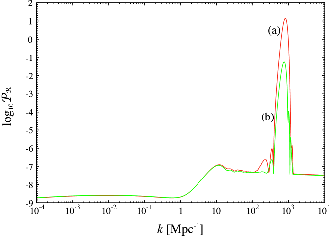
Figure 1: (a) The spectrum of primordial curvature perturbation produced by smooth hybrid new inflation, calculated under the parameter choice (32) and negligibly small decay rate $\Gamma=10^{-10}M_{G}$ of inflaton fields $\sigma$ and $\psi$. The largest peak is located at $k=810[{\mathrm{Mpc}}^{-1}]$. (b) The spectrum calculated under the same parameter choice for (a), but larger decay rate $\Gamma=6\times 10^{-8}M_{G}$.

On large scales, the spectrum has a desired shape and amplitude, although it does not agree with the best-fit parameters. The amplitude becomes large at $k=1[{\mathrm{Mpc}}^{-1}]$, and is connected to the spectrum produced by the new inflation, which has larger amplitude at $k\sim 10[{\mathrm{Mpc}}^{-1}]$. According to large scale structure observations, the spectrum is constrained to be almost flat on scales larger than $k\sim 1[{\mathrm{Mpc}}^{-1}]$. This is satisfied well by the spectrum in Fig.1-(a).

A sequence of sharp peaks is seen between $k_{0}=200[{\mathrm{Mpc}}^{-1}]$ and $k_{0}=1500[{\mathrm{Mpc}}^{-1}]$. This originates from parametric resonance, as discussed in the next section. The height of the peaks is determined by competition between parametric resonance and decay of the scalar fields $\sigma$, $\psi$. When the decay rates are large, the fluctuations ($=$ scalar particles) decay before the amplitudes are amplified through the parametric resonance, which results in suppression of the peaks in the power spectrum of the curvature perturbation. This is seen in Fig.1-(b) where the decay rates of $\sigma$ and $\psi$ are assumed to be $6\times 10^{-8}M_{G}$.

In other words, we design the height of the peaks by choosing appropriate couplings between $\sigma$($\psi$) and the standard model particles.

If we take observation of Ly-$\alpha$ into account, the amplitude of the perturbations should be small sufficiently for $k\lesssim 10[\mathrm{Mpc^{-1}}]$. The spectrum shown in Fig.2 meets this requirement. It is given under the parameter set:

$$\mu=2.04\times 10^{-3} ~{}M=1.12,~{}~{}v=5.0\times 10^{-4}$$ ,

$$m=2 ~{}n=4,~{}~{}C_{N}=0.04.$$ , (33)

At $k_{0}=0.002[{\mathrm{Mpc}}^{-1}]$, this spectrum has

$${\mathcal{R}}=4.9\times 10^{-5},~{}~{}~{}n_{s}=1.10,~{}~{}~{}\frac{dn_{s}}{d\ln k}=-0.026,$$ (34)

with $n_{s}$ and $dn_{s}/d\ln k$ at the edge of $1\sigma$ range of the WMAP three year result.

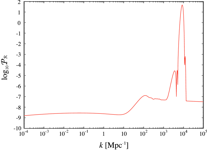
Figure 2: The spectrum of primordial curvature perturbation which is sufficiently small for $k\lesssim 10[\mathrm{Mpc^{-1}}]$. This spectrum is calculated under the parameter choice (33) and negligibly small decay rate $\Gamma=10^{-10}M_{G}$ of inflaton fields $\sigma$ and $\psi$.

IV Parametric resonance in smooth hybrid new inflation model

In this section, we will investigate the resonant amplification of fluctuations of the scalar fields $\delta\sigma_{k}$ and $\delta\psi_{k}$, and consequent amplification of $\delta\phi_{k}$. This causes a strong peak in the spectrum of primordial curvature perturbation. Since these two regimes have very different time scales, we will describe them separately.

IV.1 Parametric resonance regime

After the smooth hybrid inflation ends, $\sigma$ and $\psi$ begin to oscillate about their respective minima. We show these oscillating backgrounds in Fig.3. Hereafter, we normalize the scale factor to be $a=1$ at present.

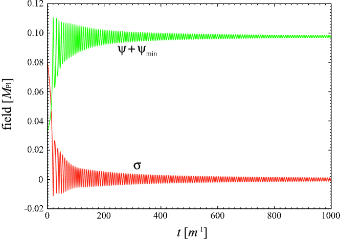
Figure 3: Oscillation of backgrounds $\sigma$ and $\psi$. Time variable $t$ is indicated in unit of $m_{\sigma}^{-1}$, here $m=m_{\sigma}\simeq m_{\psi}$. $t=0$ is taken to be $\ln a=-114.5$, at the time shortly before the oscillatory phase begins.

The evolution is very complicated. Because the cross terms which includes both $\sigma$ and $\psi$ exist in the scalar potential, $\delta\sigma_{k}$ and $\delta\psi_{k}$ contributes to the evolution of each other. Moreover, at the beginning of the oscillatory phase, the second order terms in oscillating backgrounds $\sigma$ and $\psi$ contribute to the evolution as well as the first order terms, which makes analytical understanding of parametric resonance difficult.

Retaining only the first order terms, and neglecting metric perturbations, evolution equations of $\delta\sigma_{k}$ and $\delta\psi_{k}$ are given by

$$(\delta\sigma_{k})^{\cdot\cdot}+3H(\delta\sigma_{k})^{\cdot}+\left[\frac{k^{2}}{a^{2}}+m_{\sigma}^{2}+\frac{24\mu^{2}}{M^{2}}\sqrt{\mu M}\psi\right]\delta\sigma_{k}+\frac{24\mu^{2}}{M^{2}}\sqrt{\mu M}\sigma\delta\psi_{k}=0,$$ (35)

$$(\delta\psi_{k})^{\cdot\cdot}+3H(\delta\psi_{k})^{\cdot}+\left[\frac{k^{2}}{a^{2}}+m_{\psi}^{2}+\frac{36\mu^{2}}{M^{2}}\sqrt{\mu M}\psi\right]\delta\psi_{k}+\frac{24\mu^{2}}{M^{2}}\sqrt{\mu M}\sigma\delta\sigma_{k}=0,$$ (36)

and retaining lowest order, evolution equations of backgrounds $\sigma$ and $\psi$ are given by

$$\ddot{\sigma}+3H\dot{\sigma}+m_{\sigma}^{2}\sigma=0,$$ (37)

$$\ddot{\psi}+3H\dot{\psi}+m_{\psi}^{2}\psi=0.$$ (38)

In order to understand their behaviors approximately, we will recast Eqs.(35) and (36) into following form:

$$\delta\tilde{\sigma}^{\prime\prime}+\left[A_{\sigma}-2q_{\sigma\sigma}\cos\left(2(1+d)z+\Delta\right)\right]\delta\tilde{\sigma}-2q_{\sigma\psi}\cos(2z)\delta\tilde{\psi}=0,$$ (39)

$$\delta\tilde{\sigma}^{\prime\prime}+\left[A_{\psi}-2q_{\psi\psi}\cos\left(2(1+d)z+\Delta\right)\right]\delta\tilde{\psi}-2q_{\sigma\psi}\cos(2z)\delta\tilde{\sigma}=0.$$ (40)

Here, the prime represents the derivative with respect to the variable $z$ defined as $2z=m_{\sigma}t-\pi/2$. $\Delta$ is a possible phase, and $1+d\equiv m_{\psi}/m_{\sigma}$, which satisfies $d\ll 1$. Furthermore, we approximated the oscillating background as

$$\sigma \simeq -\Sigma\sin(m_{\sigma}t),$$ (41)

$$\psi \simeq -\Psi\sin(m_{\psi}t+[\mathrm{phase~{}difference}]).$$ (42)

We also rescaled the perturbations $\delta\sigma_{k}$ and $\delta\psi_{k}$ as $\delta\tilde{\sigma}\equiv a^{3/2}\delta\sigma_{k}$ and $\delta\tilde{\psi}\equiv a^{3/2}\delta\psi_{k}$, and neglected ${\mathcal{O}}(H^{2})$ terms. The coefficients $A_{\sigma},~{}A_{\psi},~{}q_{\sigma\sigma},~{}q_{\sigma\psi},~{}q_{\psi\sigma}$, and $q_{\psi\psi}$ are given by

$$A_{\sigma}=4+\frac{4k^{2}}{a^{2}m_{\sigma}^{2}},~{}A_{\psi}=4+4\left(\frac{k^{2}}{a^{2}m_{\sigma}^{2}}+d\right),$$ (43)

$$q_{\sigma\sigma}=\frac{48\mu^{2}\sqrt{\mu M}}{M^{2}m_{\sigma}^{2}}\Psi,~{}q_{\sigma\psi}=\frac{48\mu^{2}\sqrt{\mu M}}{M^{2}m_{\sigma}^{2}}\Sigma,~{}q_{\psi\psi}=\frac{72\mu^{2}\sqrt{\mu M}}{M^{2}m_{\sigma}^{2}}\Psi.$$ (44)

At the beginning of the oscillatory phase, amplitudes are estimated as $\Sigma\sim\Psi\sim 0.01$. Neglecting $d\ll 1$, we get $A_{\sigma}\simeq A_{\psi}\simeq 4\frac{k^{2}}{a^{2}m_{\sigma}^{2}}+4\gtrsim 4$, $q_{\sigma\sigma}\simeq q_{\sigma\psi}\sim 0.62$, and $q_{\psi\psi}\sim 0.93$. Eqs.(39) and (40) look like the Mathieu equation MathieuFunctions ,

$$x^{\prime\prime}+[A-2q\cos(2z)]x=0.$$ (45)

Thus, we expect instability solutions.

To confirm the existence of the instability, we will show some results of numerical calculations. First, we have solved the coupled evolution equations (35) - (38) numerically. In order to trace evolutions of perturbations $\delta\sigma_{k}$ and $\delta\psi_{k}$ and to see the occurrence of resonant amplification, we neglected expansion of the universe: we put $H=0$.

Figure 5 and Figure 5 show time evolutions of power spectra of scalar field perturbation ${\mathcal{P}}_{\delta\sigma_{k}}$ and ${\mathcal{P}}_{\delta\psi_{k}}$ under Eqs. (35) - (38). We use $\Sigma=1.08\times 10^{-2}$ and $\Psi=1.16\times 10^{-2}$, which are evaluated at $\ln a=-114$ from the full numerical calculation of smooth hybrid new inflation given in Sec.III. Initial amplitudes $|\delta\sigma_{k}|$ and $|\delta\psi_{k}|$ are set to give $\log{\mathcal{P}}_{\delta\sigma_{k}}=0$ and $\log{\mathcal{P}}_{\delta\psi_{k}}=0$, respectively. We concentrate on two modes: $k/a\simeq 3.5\times 10^{-1}m_{\sigma}$ and $k/a\simeq 7.0\times 10^{-7}m_{\sigma}$. These modes correspond to $k=1000[{\mathrm{Mpc}}^{-1}]$ and $k=0.002[{\mathrm{Mpc}}^{-1}]$ at present. We can see that resonant amplification takes place. Rate of exponential amplification varies depending on $k$. We also find that $\delta\sigma_{k}$ and $\delta\psi_{k}$ show almost identical evolution.

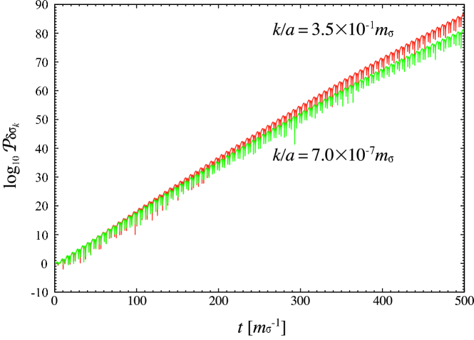
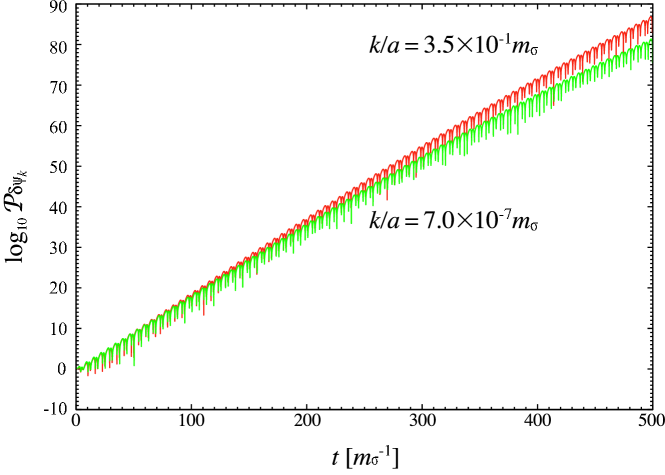
Figure 4: Time evolutions of ${\mathcal{P}}_{\delta\sigma_{k}}$ under Eqs.(35) - (38), for $k/a\simeq 3.5\times 10^{-1}m_{\sigma}$ and $k/a\simeq 7.0\times 10^{-7}m_{\sigma}$.

Figure 5: Time evolutions of ${\mathcal{P}}_{\delta\psi_{k}}$ under Eqs.(35) - (38), for $k/a\simeq 3.5\times 10^{-1}m_{\sigma}$ and $k/a\simeq 7.0\times 10^{-7}m_{\sigma}$.

Figure 6 shows scale dependence of amplification under the same configuration as that used for Fig.5. We indicate only the amplification of $\delta\sigma_{k}$, at the time $t=500m_{\sigma}^{-1}$. Since $\delta\sigma_{k}$ is oscillating rapidly, we use ${\mathcal{P}}_{\delta\sigma_{k}}|_{\mathrm{peak}}$, the peak value of oscillating ${\mathcal{P}}_{\delta\sigma_{k}}$ around at some specific moment, which is approximately equal to the amplitude of oscillation. We can see that small momentum modes $k^{2}/a^{2}\ll m_{\sigma}^{2}$ show identical amplification. Most efficient amplification takes place at $k/a\simeq 3.5\times 10^{-1}m_{\sigma}$.

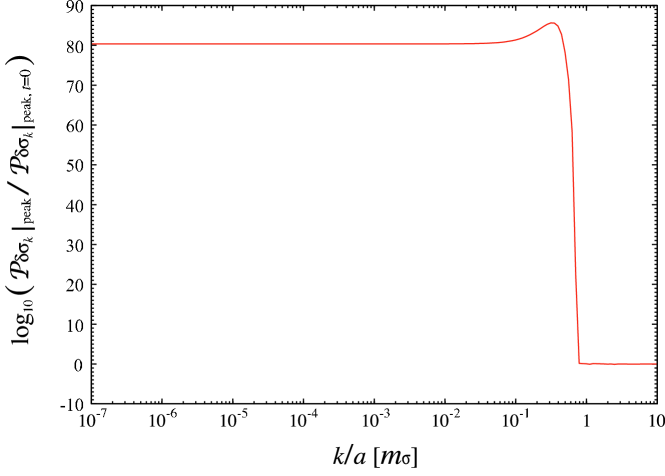
Figure 6: Scale dependence of amplification under the same configuration as that used for Fig.5 and Fig.5. We show $k$-dependence of $\left({\mathcal{P}}_{\delta\sigma_{k}}|_{\mathrm{peak}}\right)/\left({\mathcal{P}}_{\delta\sigma_{k}}|_{\mathrm{peak,t=0}}\right)$. Most efficient amplification takes place at $k/a\simeq 3.5\times 10^{-1}m_{\sigma}$, at the time $t=500m_{\sigma}^{-1}$.

Next, in order to compare the above discussion with the actual time evolution of smooth hybrid new inflation model, we numerically calculate the evolution of the fluctuation $\delta\sigma_{k}$, in the same way as described in Sec.III, solving all linear evolution equations of scalar fields Eq.(28) and metric perturbation Eq.(29) under the scalar potential $V$ given by Eqs.(23) - (26), in the expanding universe.

Figure 7 shows the mode dependence of efficiency at various times while the resonant amplification takes place. We use ${\mathcal{P}}_{\delta\sigma_{k}}|_{\mathrm{peak}}$, for the same reason that we did so for Fig.6. Since all modes of fluctuations of scalar fields decrease because of the Hubble friction term, the amplification is suppressed during the expansion of the universe, so that modes around the strong peak are amplified significantly in contrast to other modes. At $t=15m_{\sigma}^{-1}$, we can see efficient amplification of low-momentum modes. Since the effective potential of $\sigma$ is tachyonic at the end of hybrid inflation, all modes with $k^{2}/a^{2}\ll m_{\sigma}^{2}$ are amplified efficiently by tachyonic instability Felder:2000hj ; Copeland:2002ku . No significant peak appears in the spectrum of scalar perturbation at this time.

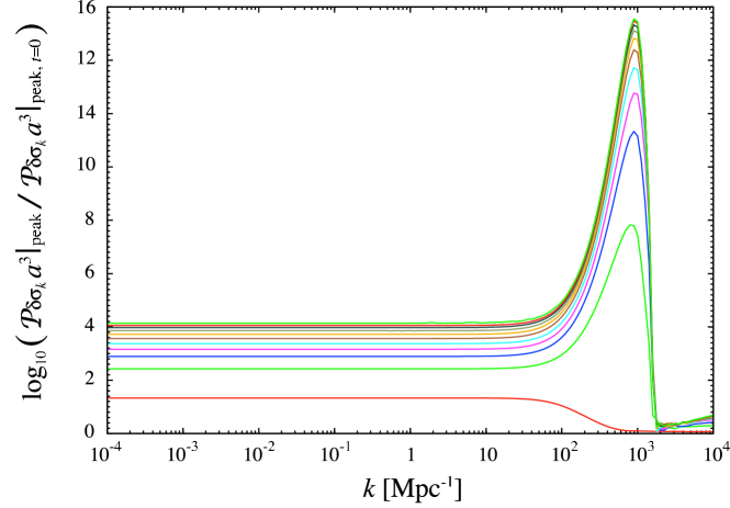
Figure 7: Scale-dependence of the resonant amplification. We show $k$-dependence of $\left({\mathcal{P}}_{\delta\sigma_{k}}a^{3}|_{\mathrm{peak}}\right)/\left({\mathcal{P}}_{\delta\sigma_{k}}a^{3}|_{\mathrm{peak,t=0}}\right)$. The bottom line indicates $t=15m_{\sigma}^{-1}$, the rest show various $t$ from $t=100m_{\sigma}^{-1}$ (next-to-bottom line) to $t=1000m_{\sigma}^{-1}$ (top line), varying by $100m_{\sigma}^{-1}$ between each lines. At $t=15m_{\sigma}^{-1}$, amplification by tachyonic instability can be seen: all modes $k/a\ll m$ are equally amplified. After that, resonant peak appears around at $k\simeq 1000[{\mathrm{Mpc}}^{-1}]$.

IV.2 Forced oscillation of $\delta\phi_{k}$

Now, we turn to the evolution of $\delta\phi_{k}$. We will focus on subhorizon modes at the beginning of oscillatory phase: $k/a>H_{H}=\mu^{2}/\sqrt{3}$ with $\ln a=-114.5$. For superhorizon modes, curvature perturbation is already frozen out, and evolution of $\delta\phi_{k}$ after smooth hybrid inflation is irrelevant.

During the smooth hybrid inflation, evolutions of $\delta\sigma_{k},\delta\psi_{k}$ and $\delta\phi_{k}$ are all dominated by $k^{2}/a^{2}$ term. They decay like $|\delta\sigma|^{2}\propto a^{-2}$ from the same initial condition given out of quantum fluctuation. So, we can estimate that $\delta\sigma_{k},\delta\psi_{k}$ and $\delta\phi_{k}$ have the same amplitude at the beginning of the oscillatory phase.

Evolution equations for Fourier modes $\delta\phi_{k}$ are given by

$$(\delta\phi_{k})^{\cdot\cdot} + 3H(\delta\phi_{k})^{\cdot}+\left[\frac{k^{2}}{a^{2}}+\frac{4\mu^{3}}{M}\psi^{2}\right]\delta\phi_{k}-\frac{2\mu}{M}\sqrt{\mu M}v^{2}\left(\psi\delta\sigma_{k}+\sigma\delta\psi_{k}\right)=0.$$ (46)

No resonant amplification due to oscillating $\sigma$ and $\psi$ occurs, since $(4\mu^{3}/M)\Psi^{2}\ll k^{2}/a^{2}\ll m^{2}$.

Let us assume sufficiently large amplification of $\delta\sigma_{k}$ or $\delta\psi_{k}$ occurs so that $(\psi\delta\sigma_{k}+\sigma\delta\psi_{k})$ terms dominates Eq.(46). The condition for that is given by

$$\left|\frac{k^{2}}{a^{2}}\delta\phi\right|\ll\left|\frac{2\mu}{M}\sqrt{\mu M}v^{2}\Psi\delta\sigma_{k}\right|.$$ (47)

In our case, this requires more than $10^{4}$ amplification of $\delta\sigma_{k}$ relative to $\delta\phi_{k}$. Since we have more than $10^{5}$ amplification at the resonant peak, this condition is satisfied very well.

Once the $(\psi\delta\sigma_{k}+\sigma\delta\psi_{k})$ term dominates Eq.(46), $\delta\phi_{k}$ undergoes forced oscillation with the source term $(\psi\delta\sigma_{k}+\sigma\delta\psi_{k})$. One can expect that this results in an amplification of $\delta\phi_{k}$, but there is another subtlety. In our case, $\psi$ and $\delta\psi_{k}$ oscillate with frequency about $m_{\psi}$, while $\sigma$ and $\delta\sigma_{k}$ oscillate with about $m_{\sigma}$. Since these two frequencies are slightly different from each other, $\psi\delta\sigma_{k}$ and $\sigma\delta\psi_{k}$ show log-period oscillatory behavior as $(C/2)\left[\cos(m_{\sigma}\delta t)-\cos\left(m_{\sigma}(2+\delta)t\right)\right]$, where $C$ is the amplitude. Then, $\delta\phi_{k}$ has a solution like

$$\delta\phi_{k}\sim-\frac{Ca^{2}}{2k^{2}}\cos(m_{\sigma}\delta t).$$ (48)

As a result, $\delta\phi_{k}$ shows long-period oscillation, whose frequency is estimated by $\Delta m$. This induces large oscillation of the amplitude of $\delta\phi_{k}$, while the mean value of oscillation is still decaying. Meanwhile, the source term decays with $|\psi\delta\sigma_{k}|\propto a^{-3}$, since $\sigma$ and $\psi$ behave as massive scalar fields. On the other hand, $H$ takes a constant value after the beginning of the new inflation. Therefore, contribution from Hubble friction term eventually becomes relevant and $\delta\phi_{k}$ ceases oscillation. Afterwards, $\delta\phi_{k}$ decays until the horizon crossing, and then it is fixed. $\delta\phi_{k}$ at that time determines the amplitude of primordial curvature perturbation:

$${\mathcal{P_{R}}}=\left(\frac{H}{\dot{\phi}}\right)^{2}{\mathcal{P}}_{\delta\phi_{k}}.$$ (49)

Since the amplitude of $\delta\phi_{k}$ is determined by the phase of large oscillation, $k$-dependence of $\delta\phi_{k}$ at horizon crossing is oscillatory. Thus, resultant spectrum of the primordial curvature perturbation has a strong peak, “sliced out” from the single resonant peak generated by parametric resonance of $\sigma$ and $\psi$ as shown in Fig.8, where we show the time evolution of $\delta\phi_{k}$ in this regime.

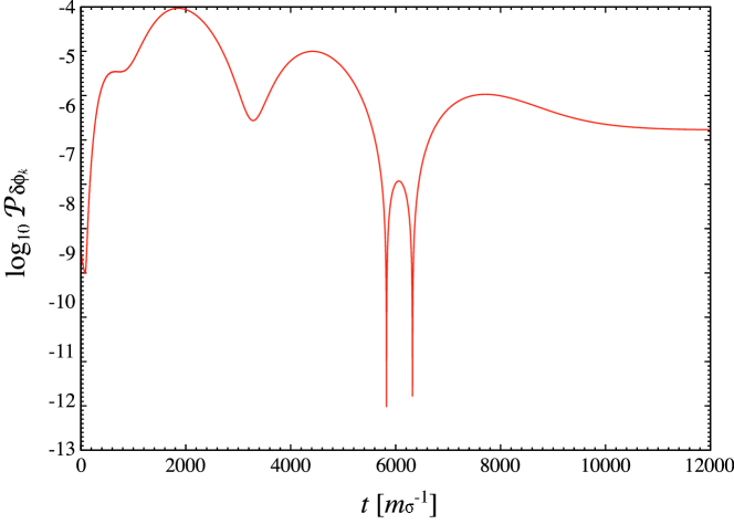
Figure 8: Long-period oscillation of ${\mathcal{P}}_{\delta\phi_{k}}$ for the mode of resonant peak: $k=810[{\mathrm{Mpc}}^{-1}]$. Sharp valley indicates that the oscillation crosses zero. The period is estimated to be $\Delta t=2\pi/\Delta m\simeq 2.6\times 10^{3}m_{\sigma}^{-1}$, which agrees well.

Let us reexamine the mechanism which induces this resonant peak by comparing estimation of the strength of peak and the result of numerical calculation.

At the beginning of long-period oscillation, the equation of motion (46) is dominated by $(k^{2}/a^{2})\delta\phi_{k}$ term and $(\psi\delta\sigma_{k}+\sigma\delta\psi_{k})$ term. Therefore we can estimate the amplitude of long-period oscillation of $\delta\phi_{k}$ from above discussion. The first peak of ${\mathcal{P}}_{\delta\phi_{k}}$ is at about $t\approx 1800m_{\sigma}^{-1}$, $\ln a\approx-111.8$. At that time, the amplitude of $\delta\sigma_{k}$ is given by ${\mathcal{P}}_{\delta\sigma_{k}}\approx 4.5\times 10^{2}$, while the amplitude of oscillating background is $\Psi\approx 3.2\times 10^{-4}$, according to the numerical calculation. We can estimate the amplitude of the long-period oscillation of $\delta\phi_{k}$, in terms of the power spectrum for $k=810[{\mathrm{Mpc}}^{-1}]$,

$${\mathcal{P}}_{\delta\hat{\phi}_{k}}\simeq\frac{a^{4}}{k^{4}}\frac{4\mu^{3}v^{4}\Psi^{2}}{M}{\mathcal{P}}_{\delta\hat{\sigma}_{k}}\simeq 1.7\times 10^{-5}.$$ (50)

Hereafter, we will concentrate on amplitudes $\hat{\delta\sigma_{k}}$ and $\hat{\delta\phi_{k}}$ of the oscillations of $\delta\sigma_{k}$ and $\delta\phi_{k}$, respectively. We approximated that the $\sigma\delta\psi_{k}$ term gives the same contribution as that of $\psi\delta\sigma_{k}$ term. The numerical calculation gives ${\mathcal{P}}_{\delta\hat{\phi}_{k}}\approx 9.3\times 10^{5}$. Our estimation is very rough, but gives the same order of the result of numerical calculation.

At the time the long-period oscillation ceases, this estimation underestimates the amplitude ${\mathcal{P}}_{\delta\hat{\phi}_{k}}$. At $t\approx 7500m_{\sigma}^{-1}$ and $\ln a\approx-108.8$, the long-period oscillation ceases, with ${\mathcal{P}}_{\delta\hat{\sigma}_{k}}\approx 3.7\times 10^{-2}$ and $\Psi\approx 3.5\times 10^{-6}$. These give ${\mathcal{P}}_{\delta\hat{\phi}_{k}}\simeq 9.9\times 10^{-8}$, while the numerical result is ${\mathcal{P}}_{\delta\hat{\phi}_{k}}\approx 1.0\times 10^{-6}$. This is because of the complexity of the evolution: since $k/aH\sim{\mathcal{O}}(1)$, the evolution is in the transition regime between subhorizon to superhorizon, and hence the evolution of $|\delta\phi_{k}|$ marginally freezes.

On the other hand, we can verify that $\delta\phi_{k}$ at the horizon crossing determines the curvature perturbation. At the horizon crossing, numerical calculation gives ${\mathcal{P}}_{\delta\hat{\phi}_{k}}\approx 3.0\times 10^{-7}$. At that time, $H\simeq 1.3\times 10^{-7}$ and $\dot{\phi}\simeq-1.3\times 10^{-11}$. We can get

$${\mathcal{P_{R}}}\bigl{|}_{\mathrm{peak}}\lesssim\left(\frac{H}{\dot{\phi}}\right)^{2}{\mathcal{P}}_{\delta\hat{\phi}_{k}}\bigl{|}_{\mathrm{cross}}\simeq 29.$$ (51)

This gives $\log{\mathcal{P_{R}}}\lesssim 1.5$ at the peak, which is the same order of the result of numerical calculation $\log{\mathcal{P_{R}}}\approx 1.15$.

V PBH formation from resonant peak

The presence of the large sharp peak around $k\simeq 10^{3}[{\mathrm{Mpc}}^{-1}]$ may lead to interesting consequences, one of which is the formation of primordial black holes. From the peak position $k=810[{\mathrm{Mpc}}^{-1}]$ of the spectrum shown in Fig.1-(a), the mean mass of resultant PBHs is estimated as

$$m_{\mathrm{BH}}=1\times 10^{9}M_{\odot}.$$ (52)

Here we assume that the whole mass within the overdense region when it enters the horizon collapses into a black hole. The abundance of such a massive PBH is constrained by assuming that they must not overclose the universe Green:1997sz . In this case, initial mass fraction $\beta$ is constrained to be $\beta<4.6\times 10^{-6}$.

We estimate the black hole abundance, following Yokoyama:1999xi based on numerical simulation of PBH formation from an overdense region Shibata:1999zs .

Assuming a spherically symmetric overdense region, two conditions must be satisfied for the formation of PBHs from the overdense region. First, the overdense region must have larger density than a critical value. Under the linear approximation, this is given by curvature perturbation at the horizon crossing ${\mathcal{R}}(t,r)$ as

$${\mathcal{R}}(t,0)\gtrsim 0.67~{}:~{}~{}{\mathrm{C1}}.$$ (53)

The other independent condition is given by

$$-0.72\lesssim X(r)\lesssim-0.28~{}:~{}~{}{\mathrm{C2}},$$ (54)

where $X(r)=\frac{r}{2}\frac{d{\mathcal{R}}}{dr}$ at the horizon crossing. The latter condition requires that the excess mass around the overdense regin is sufficiently large. The initial mass fraction $\beta$ of PBHs can be identified with the probability $P({\mathrm{C1}}\cap{\mathrm{C2}})$. Assuming that the density perturbation has a Gaussian probability distribution, the probability $P({\mathrm{C1}})$ is given by

$$P({\mathrm{C1}})=\int_{0.67}\frac{1}{\sqrt{2\pi}\sigma_{\mathcal{R}}}\exp\left(-\frac{\delta^{2}}{2\sigma^{2}_{\mathcal{R}}}\right)d\delta,$$ (55)

where $\sigma_{\mathcal{R}}$ is the variance of ${\mathcal{R}}$ at the horizon crossing. For the spectrum shown in Fig.1-(a), we can get $\sigma_{\mathcal{R}}=1.9$, which results in $\beta\simeq 0.35$.

On the other hand, under the presence of a peak with ${\mathcal{R}}(t,0)=0.67$, the conditional probability of $({\mathrm{C2}})$ is found to be 0.5. Consequently, the initial mass fraction of PBHs is estimated to be

$$\beta\simeq P({\mathrm{C1}}\cap{\mathrm{C2}})\sim 0.18.$$ (56)

This is far larger than the constraint $\beta<4.6\times 10^{-6}$.

If we introduce larger decay rates of inflaton fields $\sigma$ and $\psi$, resultant PBH abundance can be acceptably small. The spectrum shown in Fig.1-(b) gives $\beta\sim 5.6\times 10^{-9}$, which is below the bound $\beta<4.6\times 10^{-6}$.

VI Conclusion and Discussion

We have reexamined the smooth hybrid new inflation model, which was designed to reproduce the running spectral index suggested by the WMAP three year result, by numerical calculation of the perturbation. We have confirmed that this model can reproduce the spectrum within 1$\sigma$ range of the WMAP three year result.

In addition, we find strong peaks on smaller scales, which originate from the amplification of perturbation $\delta\phi$ and $\delta\psi$ by parametric resonance. Since there are interactions between $\sigma,\psi$ and $\phi$, this amplified perturbation is transfered to $\delta\phi$. $\delta\phi$ begins large-amplitude and long-period oscillation, and freezes out at the horizon crossing, determining the primordial curvature perturbation. The resultant curvature perturbation depends on the phase of oscillating $\delta\phi$, so that the resonant peak consists of several steep peaks and valleys. The strength of the resultant peak can be controlled by the decay rate of the first inflaton, and the comoving scale of the peak can be controlled by the scale factor at the beginning of oscillatory phase.

Such a peak in the spectrum of primordial curvature perturbation can be a source of PBHs. Due to the strong peak, mass of generated PBHs can be estimated by the horizon mass at the horizon crossing of the scale which corresponds to the resonant peak.

- (1) D. N. Spergel et al. [WMAP Collaboration], Astrophys. J. Suppl. 148, 175 (2003).
- (2) H. V. Peiris et al., Astrophys. J. Suppl. 148, 213 (2003).
- (3) A. Slosar and U. Seljak, Phys. Rev. D 70, 083002 (2004).
- (4) D. N. Spergel et al., [arXiv:astro-ph/0603449].
- (5) U. Seljak et al. [SDSS Collaboration], Phys. Rev. D 71, 103515 (2005).
- (6) G. Ballesteros, J. A. Casas and J. R. Espinosa, JCAP. 0603, 001 (2006).
- (7) C.-Y. Chen, B. Feng, X.-L. Wang, and Z.-Y. Yang, Class. Quant. Grav. 21, 3223 (2004).
- (8) M. Kawasaki, M. Yamaguchi, and J. Yokoyama, Phys. Rev. D 68, 023508 (2003).
- (9) M. Yamaguchi and J. Yokoyama, Phys. Rev. D 68, 123520 (2003).
- (10) M. Yamaguchi and J. Yokoyama, Phys. Rev. D 70, 023513 (2004).
- (11) G. Lazarides and C. Panagiotakopoulos, Phys. Rev. D 52, R559 (1995).
- (12) K. Kumekawa, T. Moroi, and T. Yanagida, Prog. Theor. Phys. 92, 437 (1994).
- (13) K. I. Izawa and T. Yanagida, Phys. Lett. B 393, 331 (1997).
- (14) M. Ibe, K. I. Izawa, Y. Shinbara, and T. T. Yanagida, [arXiv:hep-ph/0602192].
- (15) L. Kofman, A. D. Linde, and A. A. Starobinsky, Phys. Rev. Lett. 73, 3195 (1994).
- (16) Y. Shtanov, J. H. Traschen, and R. H. Brandenberger, Phys. Rev. D 51, 5438 (1995).
- (17) L. Kofman, A. D. Linde, and A. A. Starobinsky, Phys. Rev. D 56, 3258 (1997).
- (18) M. Yamaguchi and J. Yokoyama, [arXiv:hep-ph/0512318].
- (19) M. Kawasaki and T. Yanagida, Phys. Rev. D 59, 043512 (1999).
- (20) D. S. Salopek, J. R. Bond, and J. M. Bardeen, Phys. Rev. D 40, 1753 (1989).
- (21) N.W.MacLachlan, Theory and Application of Mathieu Functions, Dover, New York (1961).
- (22) G. N. Felder, J. Garcia-Bellido, P. B. Greene, L. Kofman, A. D. Linde, and I. Tkachev, Phys. Rev. Lett. 87, 011601 (2001).
- (23) E. J. Copeland, S. Pascoli, and A. Rajantie, Phys. Rev. D 65, 103517 (2002).
- (24) A. M. Green and A. R. Liddle, Phys. Rev. D 56, 6166 (1997).
- (25) J. Yokoyama, Prog. Theor. Phys. Suppl. 136, 338 (1999).
- (26) M. Shibata and M. Sasaki, Phys. Rev. D60, 084002 (1999).