Maximum Significance at the LHC and Higgs Decays to Muons

Abstract

We present a new way to define and compute the maximum significance achievable for signal and background processes at the LHC, using all available phase space information. As an example, we show that a light Higgs boson produced in weak–boson fusion with a subsequent decay into muons can be extracted from the backgrounds. The method, aimed at phenomenological studies, can be incorporated in parton–level event generators and accommodate parametric descriptions of detector effects for selected observables.

The Large Hadron Collider (LHC) will have a tremendous capacity to search for new particles, such as the Standard Model Higgs boson or new particles suggested by various scenarios for physics beyond the Standard Model. For such searches, it is important to asses the experimental sensitivity, which requires a description of the experimental search technique to isolate signal-rich data. Traditionally, this has been accomplished by using ad hoc kinematic cuts. At the parton–level this process of designing cuts by hand to isolate signal-enhanced phase space regions (which emulates the traditional experimental practice) is not necessary. In this paper we present a new method of computing the statistical significance of a hypothesized signal via direct integration of the likelihood ratio. This technique does not require identification of powerful discriminating variables or techniques to estimate probability density functions from a discrete sample of events. Instead, we compute the likelihood ratio exactly over the full phase space, which implies that this expected significance is an upper bound. This maximal significance indicates if a more detailed study with a full detector simulation is warranted and provides a target significance to which any experimental study can be compared.

To demonstrate the power of this method, we consider the production of the Standard Model Higgs boson at the LHC via weak–boson fusion with a subsequent decay to muons. Weak–boson fusion production of a Higgs boson with a subsequent decay to tau leptons originally proposed in Ref. wbf_tau has been firmly established by Atlas and CMS as the main discovery channel for a light Higgs boson in the Standard Model karl as well as in its supersymmetric extension wbf_mssm . While QCD effects can be a danger for most LHC analyses, additional jet radiation turns into a useful tool in the case of weak–boson fusion signals wbf_minijet . Observation of the same process with a decay to muons can experimentally confirm Yukawa couplings and their scaling with the masses for non–third–generation fermions.

The expected significance of a search for $H\to\mu\mu$ was estimated for weak–boson fusion wbf_muon and gluon fusion gg_muon production modes. For a 120 GeV Higgs boson mass, the best kinematic cuts found in Ref. wbf_muon result in a $1.8~{}\sigma$ significance. The authors of that analysis note that many observables display additional discriminating power and suggest that neural networks or other multivariate procedures could enhance the sensitivity. Using our new method we find that the maximum possible (target) significance for $H\to\mu\mu$ is much higher, i.e. the cut analysis can indeed be significantly improved.

.1 Neyman–Pearson Lemma

Our approach is based on the Neyman–Pearson lemma: the likelihood ratio is the most powerful variable or test statistic for a hypothesis test between a simple (i.e. having no free parameters) null hypothesis — background only — and an alternate hypothesis — signal plus background Kendall . Maximum power is formally defined as the minimum probability for a Type II error (false negative) for a given probability for a Type I error (false positive). If we assume that the signal–plus–background hypothesis is true, the most powerful method has the lowest probability of mistaking the signal for a background fluctuation.

The Neyman–Pearson lemma is commonly used to claim optimality, but these claims can be misleading. The reason is that the probability density function (pdf) of a multi-dimensional observable $x$ for a given hypothesis is not experimentally known. Instead, experimentalists typically use a discrete sample of events $\{x_{i}\}$ to approximately estimate the pdf kernel . In practice, the size of the sample limits the dimensionality of the pdf that can be estimated to one or two dimensions, or it requires one to neglect correlations among the observables – both of which invalidate strict claims of optimality. In contrast, in phenomenology we can use the parton–level transition amplitude for a process (at a given order in perturbation theory) to exactly compute the pdf over the full phase space.

Two main ingredients are needed to calculate the distribution of the likelihood ratio for the background–only and signal–plus–background hypotheses. First, we have to evaluate identical sets of phase space points for signal and background processes, which is not part of standard Monte Carlo event generators. Secondly, we need to bootstrap the likelihood ratio distribution for one event to the distribution for a fixed luminosity including Poisson fluctuations. Both ingredients are discussed in the next Section. We then consider an example: a light Higgs boson produced via weak–boson fusion and decaying to muons. To achieve a minimum level of realism, we generalize our method to include experimental resolutions and detector effects.

It should be noted that this work builds on several techniques used in experimental analyses, but it extends that work and applies it in a phenomenological context. For instance, the literature is replete with measurement techniques that use - to varying degrees - the matrix element to describe kinematic distributions earlyDLmethod ; optimalObservables ; LEPExample . A qualitative distinction of this work is that we are estimating the sensitivity of a search for a hypothesized particle instead of measuring a theoretical parameter with data (e.g. the mass of the top quark or the helicity of the $W$ boson). In particular, we are not trying to identify the maximum–likelihood estimator for a parameter to be extracted from data. The process of evaluating the likelihood of an event in real data is significantly different from constructing hypothetical data sets, and this leads to significant differences in the implementation of the algorithms (in particular, the two main ingredients mentioned in the previous paragraph). Our approach to the incorporation of experimental resolutions is very similar to the recent work at the Tevatron, generically referred to as “matrix element method” WHelicity ; DLmethod ; MEmethod , and we try to use similar notation and terminology to make the correspondence clear. Furthermore, we build on the statistical techniques (e.g. Eqs. 2-5) used in the LEP Higgs working group lepewwg , which generally has not been matched with the matrix element method.

In short, our method is a novel combination of the LEP statistical formalism with parton–level transition amplitudes used to define and compute a mathematically well defined maximum expected significance. Note that we do not attempt to identify any powerful discriminating observables, nor do we attempt to compute an observed significance based on experimental data bard . Instead, we formulate and answer the question: what is the maximum expected significance of a potential physics signal, e.g. a Higgs decaying to muons?

.2 Likelihood Ratio and Discovery Potential

We first limit ourselves to a signal process and its irreducible backgrounds, i.e. signal and background processes with identical degrees of freedom in the final state, distinguished by (kinematic) distributions. To compute the expected signal and background rates we integrate the matrix elements squared over the phase space, with or without (acceptance) cuts, using a Monte Carlo integration. This method probes the phase space with random numbers. Ideally, the dimension of the random number vector $\vec{r}$ is given by the number of degrees of freedom in the final–state momenta after all kinematic constraints. The random number vector forms a (minimal) basis for all final-state configurations. We can schematically write

$$\sigma_{\rm tot}=\int_{\rm cuts}dPS\;M_{PS}\;d\sigma_{PS}=\int_{\rm cuts}d\vec{r}\;M({\vec{r}})\;d\sigma({\vec{r}})$$ (1)

where the phase space boundaries are included in the integral, and the differential cross section $d\sigma(\vec{r})$ includes all phase space factors and the Jacobian for transforming the integration to the random–number basis. The integration over the parton distributions is included in the phase space integral. The measurement function $M$ can be used to include additional cuts or to incorporate event weights (e.g. particle identification efficiencies) as a function of any observable. Removing unwanted parts of the phase space through cuts on observable quantities consistently removes the contribution of these phase space regions from all proccesses. Because the random numbers parameterize the entire phase space, all potentially available information about the process is included in the array of event weights $(M\,d\sigma)({\vec{r}})$. Note that this phase space integration above is written assuming a simple cross section expression $d\sigma$; however, it can be replaced with any combination of differential cross sections which modern parton–level event generators predict.

A cut analysis defines a signal–rich region bounded by upper and lower limits on observables and then counts events in that region. Ultimately, the variable that discriminates between signal and background — the test statistic — is simply the number of events observed in this region. Predicting the expected number of background events $b$ and signal events $s$ enables us to adjust the cut values which optimize the experimental sensitivity. More sophisticated techniques use multivariate algorithms, such as neural networks, to define more complicated signal–like regions, but the test statistic often remains unchanged. In all of these counting analyses, the likelihood of observing $n$ events assuming the background-only hypothesis is simply given by the Poisson distribution ${\rm Pois}(n|b)=e^{-b}\,b^{n}/n!$.

There are extensions to this number counting, assuming we know the distribution of a discriminating observable $x$ (which may be multi-dimensional). We assume that for the background–only hypothesis $H_{0}$ this distribution is $f_{b}(x)$, while for the signal–plus–background hypothesis $H_{1}$ it is $f_{s+b}(x)=\left[sf_{s}(x)+bf_{b}(x)\right]/(s+b)$ assuming no interference. Following the Neyman-Pearson lemma, the most powerful test statistic is the likelihood ratio for the entire experiment’s data. The total likelihood for the full–experiment observable ${\bf x}=\{x_{j}\}$ can be factorized into the Poisson likelihood to observe $n$ events, and the product of the individual event’s likelihood $f(x_{j})$:

$$Q({\bf x}) =\frac{L({\bf x}|H_{1})}{L({\bf x}|H_{0})}=\frac{{\rm Pois}(n|s+b)\;\prod_{j=1}^{n}f_{s+b}(x_{j})}{{\rm Pois}(n|b)\;\prod_{j=1}^{n}f_{b}(x_{j})}=e^{-s}\;\left(\frac{s+b}{b}\right)^{n}\;\frac{\prod_{j=1}^{n}f_{s+b}(x_{j})}{\prod_{j=1}^{n}f_{b}(x_{j})}$$

$$q({\bf x}) \equiv\ln Q({\bf x})={-s}+\sum_{j=1}^{n}\ln\left(1+\frac{sf_{s}(x_{j})}{bf_{b}(x_{j})}\right)$$ (2)

We compute the normalized probability distributions $f(x)$ from the parton–level matrix elements. This way we construct a log–likelihood ratio map of all possible final–state phase space configurations using the normalized probability distributions $d\sigma(\vec{r})/\sigma_{\rm tot}$ for the signal and background hypotheses:

$$q(\vec{r})=-\sigma_{{\rm tot},s}\;{\cal L}\;+\,\ln\left(1+\frac{d\sigma_{s}(\vec{r})}{d\sigma_{b}(\vec{r})}\right)$$ (3)

${\cal L}$ is the integrated luminosity. To construct the single–event probability distribution $\rho_{1,b}(q)$ we combine the background event weight with the log–likelihood ratio map $q(\vec{r})$ from Eq.(3), which in general is not invertable:

$$\rho_{1,b}(q_{0})=\int d\vec{r}\;\frac{d\sigma_{b}(\vec{r})}{\sigma_{{\rm tot},b}}\;\delta\left(q(\vec{r})-q_{0}\right)$$ (4)

For multiple events, the distribution of the log–likelihood ratio $\rho_{n,b}$ can be computed by repeated convolutions of the single event distribution. This convolution we can either perform implicitly with approximate Monte Carlo techniques junk , or analytically using a Fourier transform clfft .

The expected log–likelihood ratio distribution for a background including Poisson fluctuations in the number of events takes the form $\rho_{b}(q)=\sum_{n}{\rm Pois}(n|b)\times\rho_{n,b}(q)$. To compute this $\rho_{b}(q)$ from the single–event likelihood $\rho_{1,b}(q)$ given by Eq.(4) we first Fourier transform all $\rho$ functions into complex–valued functions of the Fourier conjugate of likelihood ratio, e.g. $\overline{\rho_{1,b}}(\overline{q})$. The Fourier–transformed $n$-event likelihood ratio is now given by $\overline{\rho_{n,b}}=(\overline{\rho_{1,b}})^{n}$ equivalent to a convolution in $q$-space. The sum over $n$ in the formula for $\rho_{b}(q)$ now has a simple form in the Fourier domain: $\overline{\rho_{b}}=\exp[b\;(\overline{\rho_{1,b}}-1)]$. For the signal–plus–background hypothesis we expect $s$ events from the $\rho_{1,s}$ distribution and $b$ events from the $\rho_{1,b}$ distribution. Similar to the above formula we have $\overline{\rho_{s+b}}=\exp[b(\overline{\rho_{1,b}}-1)+s(\overline{\rho_{1,s}}-1)]$. This form we can transform back and obtain the log-likelihood ratio distributions $\rho_{b}(q)$ and $\rho_{s+b}(q)$.

Given a log-likelihood ratio $q$ we can calculate the background-only confidence level, ${\rm CL}_{b}$:

$${\rm CL}_{b}(q)=\int_{q}^{\infty}dq^{\prime}\;\rho_{b}(q^{\prime})$$ (5)

To estimate the discovery potential of a future experiment we assume the signal–plus–background hypothesis to be true and compute ${\rm CL}_{b}$ for the median of the signal–plus–background distribution $q^{*}_{s+b}$. This expected background confidence level can be converted into an equivalent number of Gaussian standard deviations and the significance written as $Z~{}\sigma$ by implicitly solving ${\rm CL}_{b}(q^{*}_{s+b})=\left(1-{\rm erf}(Z/\sqrt{2}\right)/2$ for $Z$.

.3 Higgs Decay to Muons

Figure 1: Normalized $\rho_{b}(q)$ and $\rho_{s+b}(q)$ distributions, corresponding to the full–experiment log–likelihood ratio in Eq.(2). These distributions define the expected significance.

To determine the maximal significance in a strict sense we should not include detector effects which always decrease the significance. However, in our example of weak–boson–fusion $H\to\mu\mu$ the experimental resolution on the invariant mass $m_{\mu\mu}$ is much larger than the Higgs width: about 1.6 $~{}{\rm GeV}$ for CMS and 2.0 $~{}{\rm GeV}$ for Atlas massResolution . To obtain a semi–realistic result we introduce a Gaussian smearing for $m_{\mu\mu}$ into Eq.(1). This Gaussian shape is just a simple numerical choice and could be replaced with any other smearing prescription or fast detector simulation. We convolute our momentum smearing with the Breit–Wigner–shaped Higgs propagator; in our case, the combination is completely dominated by the much larger Gaussian width.

We introduce a new random number $r_{m}^{*}$ corresponding to the smeared $m_{\mu\mu}^{*}$ and integrate over a transfer function from the true $m_{\mu\mu}$ to the smeared $m_{\mu\mu}^{*}$ by aligning one of the original random numbers $r_{m}$ with $m_{\mu\mu}$:

$$\sigma_{\rm tot}=\int d\vec{r}_{\perp}dr_{m}^{*}\int_{-\infty}^{\infty}dr_{m}\;M({\vec{r}})\;d\sigma({\vec{r}})\;W(r_{m},r_{m}^{*})$$ (6)

The original random number vector $\vec{r}$ is split into $\vec{r}=\{\vec{r}_{\perp},r_{m}\}$. In our case, the transfer function $W$ is a normalized Gaussian giving the likelihood to reconstruct $m_{\mu\mu}^{*}$ given the true $m_{\mu\mu}$ and the experimental mass resolution. We trivially get back Eq.(1) for $W(r_{m},r_{m}^{*})\to\delta(r_{m}-r_{m}^{*})$.

In general one must be careful about the mapping between parton–level quantities and their observable counter-parts. As in most experimental analyses that use the matrix element method, the jet direction is assumed to be well-measured. We do not include a jet energy scale in the transfer function $W$, because, unlike the top-mass measurement with a hadronically decaying resonance, the jet energy scale is not a dominant experimental issue for this search. In particular, the jet momenta have relatively flat distributions, i.e. their variation on the scale of detector effects is small wbf_muon . In the general case, one should consider all permutations between out-going quarks and gluons with jets; however, in the case of weak boson fusion, the signal-like regions of phase space have more than three units of pseudorapidity separating the tagging jets, which makes the association of parton to jet unambiguous. In other words, adding the alternative jet–parton assignment would give a negligible contribution to the event weight. The correspondence of the muons is also clear due to their charge.

From Eq.(1) it is obvious how to include an experimental mass resolution: we replace the event weights $(M\,d\sigma)$ by the integral $\left(M\int dr_{m}\,d\sigma\,W\right)$ and evaluate them over the smeared phase space $\{\vec{r}_{\perp},r_{m}^{*}\}$. Because the random numbers form a (minimal) basis for all final state configurations there is no ‘back door’ for the true (infinitely well measured) $m_{\mu\mu}$ to enter the likelihood calculation. A rough approximation to incorporating the $m_{\mu\mu}$ mass resolution could be an increased physical Higgs width. It replaces the Gaussian smearing with a Breit–Wigner function; we compared this approximate method with the proper smearing procedure and found that the difference in the final results was small but not negligible.

For all details of the signal and background simulation (using CTEQ 5L parton distributions) we refer to Ref. wbf_muon . There, after very basic cuts the signal cross section for a $120~{}{\rm GeV}$ Higgs is $0.22~{}{\rm fb}$, hidden under $0.33~{}{\rm fb}$ of electroweak $Z$ production and $2.6~{}{\rm fb}$ of QCD $Z$ production, where the $Z$ decays into muons. All other backgrounds combined contribute less than $0.01~{}{\rm fb}$, which allows us to neglect them. It is worth mentioning that the electroweak $Z$ production consists of as many as 48 diagrams for a fixed flavor configuration, which is substantially more complicated than the search for single top production singleTop . Conservatively assuming no additional information from higher–order jet radiation, we could apply $K$ factors to the signal and cross section rates, but this would lead beyond this proof–of–principle letter.

To probe the likelihood ratio over the full phase space, we relax the cuts for a $120~{}{\rm GeV}$ Standard Model Higgs to mere acceptance cuts. All cross sections are finite, so the cut values have no effect on the likelihood we obtain. Using $2^{20}$ points we integrate over the final–state phase space projected onto the log–likelihood ratio $q(\vec{r})$ according to Eq.(4). The phase space points used for this integration are defined by the same grid we use for the integration over the signal and background amplitudes described in Eq.(6); this way we can check the total rates to ensure that the likelihood integration covers the entire phase space. For each phase space point we integrate over the true $m_{\mu\mu}$ as shown in Eq.(6), using a proper phase space mapping. Note that this internal integration does not have to use the same grid for signal and background.

The resulting log-likelihood distributions $\rho_{b}(q)$ and $\rho_{s+b}(q)$ are shown in Fig. 1. From the background pdf we extract the signal significance for an integrated luminosity of $300~{}{\rm fb}^{-1}$ as $3.54~{}\sigma$ for CMS and $3.19~{}\sigma$ for Atlas. Note that this significance estimate neglects theoretical uncertainty in the overall rate since the signal has small higher-order corrections wbf_qcd and the normalization of the background will be well measured with $300~{}{\rm fb}^{-1}$ of data. Also note that this significance does not include a minijet veto because only two jets are included in our parton–level transition amplitude; in principle, the same procedure could be repeated with a higher-order tree-level or a next-to-leading order calculation. Following Ref. wbf_muon we can estimate the effect of a minijet veto, which increases the significance to $\sim 4.4~{}\sigma$ for CMS. Survival probabilities for the veto neglect pile-up effects, which will degrade the enhancement in significance. Combining both experiments the significance even without a minijet veto is $4.77~{}\sigma$.

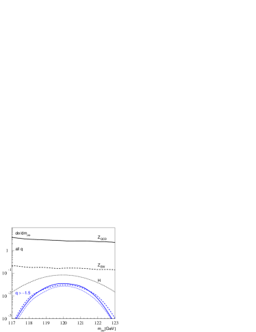
Figure 2: Muon invariant mass distribution for the 120 GeV Higgs signal and $Z$+jets background with acceptance cuts only (upper curves) and after a cut on the log–likelihood ratio $q(\vec{r})>-1.5$ (lower curves). The curves correspond to CMS and illustrate that events with high $q(\vec{r})$ have an increased signal purity and signal–like characteristics.

The most relevant kinematic distribution is the reconstructed Higgs mass $m_{\mu\mu}$. In the upper curves of Fig. 2 we show it for signal and backgrounds without kinematic or likelihood cuts. The signal shows a smeared mass peak, while the backgrounds are flat. To illustrate how the method isolates signal–rich phase space regions, we apply a likelihood ratio cut $q(\vec{r})>-1.5$. Roughly a third of the signal events survive this cut, and each of the backgrounds are reduced to a rate comparable to the signal. After the likelihood cut the backgrounds show the same kinematic features as the signal, i.e. a peak in $m_{\mu\mu}$.

.4 Detector Effects and Reducible Backgrounds

The procedure for incorporating detector smearing on observables described above is tailored for smearing of a few observables, which are isolated in the phase space integration. Nevertheless, it is possible to generalize the smearing procedure. In essence, a complete detector smearing requires an integration over a fixed set of experimental observables with a nested integration over the remaining degrees of freedom in the phase space. The latter include the unsmeared (true) observables, as shown in Eq.(6), as well as the unobservable longitudinal component of neutrino momenta at a hadron collider or the momentum of particles not passing the acceptance cuts. As mentioned in the previous section and discussed in the literature related to the matrix element method, one should take care to include in the transfer function all relevant detector effects and consider all permutations that arise from ambiguities in the mapping from parton–level quantities to their final state observables.

We usually include detector effects by smearing all final state four-momenta; however, this can be computationally inefficient. If we instead choose not to smear some of the observables, we must remain vigilant to insure that there is no ‘back door’ through which four-momentum conservation together with unsmeared observables implicitly evade smearing. We avoid this ‘back door’ explicitly in Eq.(6) by factorizing the basis of the phase space into orthogonal components $r_{m}$ and $r_{\perp}$.

After generalizing our method to smear multiple observables we can now incorporate reducible backgrounds, i.e. background whose final–state configurations have more degrees of freedom than the signal. We simply pick a set of observables that is common to all signal and background processes, and marginalize the additional background degrees of freedom. Flavor tagging efficiencies and fake rates can be included in the event weights through $W$. In these scenarios, the interpretation of the resulting significance is more vague: it is the maximal significance given the specified set of observables and the assumptions in the transfer and measurement functions.

.5 Conclusions

We have described a way to compute the mathematically strict maximum significance for a set of signal and background processes at the parton–level. Our method is based on the Neyman–Pearson lemma and can be used to decide if a new physics search at high–energy colliders has a sufficiently large discovery potential to justify a dedicated analysis.

While our example is fairly simple, including only irreducible backgrounds and incorporating experimental resolution for only a single observable, we have outlined the extension of the method to include general detector effects. This approach to including detector effects follows closely the recent experimental work at the Tevatron referred to as ‘the matrix element method’. The next step will be to implement this likelihood computation into a parton–level event generator with a simple and fast simulation of detector effects whizard .

Weak–boson–fusion production of a Higgs boson with a subsequent decay to muons is the perfect showcase for this new method: it suffers from very low signal rate and from the lack of distributions that clearly distinguish signal from background. A very basic cut analysis in Ref. wbf_muon quotes a significance of $1.8~{}\sigma$ for $300~{}{\rm fb}^{-1}$ for a single experiment. In particular, Ref. wbf_muon found that a cut analysis was likely not the best–suited strategy for this signal. Applying our method we arrive at a possible maximum significance of $3.54~{}\sigma$ (CMS with $300~{}{\rm fb}^{-1}$). By increasing the complexity of the final state, higher–order QCD effects can be exploited using a minijet veto wbf_minijet , which could increase the significance to $\sim 4.4~{}\sigma$. Not only is this result grounds for a more careful study by the experimental collaborations, but it also indicates that without a luminosity upgrade Atlas and CMS combined may be able to observe the decay $H\to\mu\mu$.

- (1) D. L. Rainwater, D. Zeppenfeld and K. Hagiwara, Phys. Rev. D 59, 014037 (1999), T. Plehn, D. L. Rainwater and D. Zeppenfeld, Phys. Rev. D 61, 093005 (2000).
- (2) for recent overviews see e.g. : A. Djouadi, arXiv:hep-ph/0503172; S. Asai et al., Eur. Phys. J. C 32S2, 19 (2004); V. Büscher and K. Jakobs, Int. J. Mod. Phys. A 20, 2523 (2005).
- (3) T. Plehn, D. L. Rainwater and D. Zeppenfeld, Phys. Lett. B 454, 297 (1999).
- (4) V. D. Barger, K. m. Cheung, T. Han and R. J. N. Phillips, Phys. Rev. D 42, 3052 (1990); D. L. Rainwater, R. Szalapski and D. Zeppenfeld, Phys. Rev. D 54, 6680 (1996); V. Del Duca et al., arXiv:hep-ph/0608158.
- (5) T. Plehn and D. L. Rainwater, Phys. Lett. B 520, 108 (2001).
- (6) T. Han and B. McElrath, Phys. Lett. B 528, 81 (2002); E. Boos, A. Djouadi and A. Nikitenko, Phys. Lett. B 578, 384 (2004).
- (7) for a proof and corresponding definitions, see e.g. : J. Stuart, A. Ord and S. Arnold, Kendall’s Advanced Theory of Statistics, Vol 2A (6th Ed.) (Oxford University Press, New York, 1994); for a pedagogical introduction in the context of high-energy physics, see A. Read, in ‘1st Workshop on Confidence Limits’, CERN Report No. CERN-2000-005 (2000).
- (8) K. S. Cranmer, Comput. Phys. Commun. 136, 198 (2001).
- (9) R. Barate et al. [LEP Working Group for Higgs boson searches Collaboration], Phys. Lett. B 565, 61 (2003).
- (10) K. Kondo, J. Phys. Soc. Jpn. 57, 4126 (1988).
- (11) D. Atwood and A. Soni, Phys. Rev. D 45, 2405 (1992); M. Diehl and O. Nachtmann, Eur. Phys. J. C 1, 177 (1998).
- (12) P. Abreu et al. [DELPHI Collaboration], Eur. Phys. J. C 2, 581 (1998).
- (13) V. M. Abazov et al. [D0 Collaboration], Phys. Lett. B 617, 1 (2005).
- (14) A. Abulencia et al. [CDF Collaboration], Phys. Rev. D73, 092002 (2006).
- (15) V.M Abazov et. al., [D0 Collaboration], Nature 429, 638 (2004)
- (16) V. M. Abazov [D0 Collaboration], [arXiv:hep-ex/0612052].
- (17) B. Knuteson and S. Mrenna, arXiv:hep-ph/0602101; B. McElrath et al., in preparation.
- (18) T. Junk, Nucl. Instrum. Meth. A 434, 435 (1999).
- (19) H. Hu and J. Nielsen, in ‘1st Workshop on Confidence Limits’, CERN 2000-005 (2000) [arXiv:physics/9906010].
- (20) Atlas Muon TDR CERN/LHCC 97-22 (1997); CMS Muon TDR CERN/LHCC 97-32 (1997).
- (21) T. Han, G. Valencia and S. Willenbrock, Phys. Rev. Lett. 69, 3274 (1992); T. Figy, C. Oleari and D. Zeppenfeld, Phys. Rev. D 68, 073005 (2003);
- (22) K. Cranmer, T. Plehn, J. Reuter and D. Rainwater, in preparation.