UNIVERSITÀ DEGLI STUDI DI LECCE
DIPARTIMENTO DI FISICA
![[Uncaptioned image]](/html/hep-ph/0605241/assets/x1.png)
QCD at Hadron Colliders and in
Ultra High Energy Cosmic Rays
Advisor
Claudio Corianò
| Candidate |
| Alessandro Cafarella |
Tesi di Dottorato di Ricerca in Fisica – XVII Ciclo
List of publications
Research papers
The chapters presented in this thesis are based on the following research works.
-
1.
A. Cafarella, C. Corianò and M. Guzzi, An -space analysis of evolution equations: Soffer’s inequality and the nonforward evolution, J.High Energy Phys. 11 (2003) 059
-
2.
A. Cafarella and C. Corianò, Direct solution of renormalization group equations of QCD in -space: NLO implementations at leading twist, Comput.Phys.Commun. 160 (2004) 213
-
3.
A. Cafarella, C. Corianò and A. Faraggi, Large scale air shower simulations and the search for new Physics at Auger, Int.J.Mod.Phys.A 19, 22 (2004) 3729
-
4.
A. Cafarella, C. Corianò and T.N. Tomaras, Cosmic ray signals from mini black holes in models with extra dimensions: an analytical/Monte Carlo study, J.High Energy Phys. 06 (2005) 065
-
5.
A. Cafarella and C. Corianò, The kinetic interpretation of the DGLAP equation, its Kramers-Moyal expansion and positivity of helicity distributions, Int.J.Mod.Phys.A 20, 21 (2005) 4863
-
6.
A. Cafarella, C. Corianò, M. Guzzi and J. Smith, On the scale variation of the total cross section for Higgs production at the LHC and at the Tevatron, hep-ph/0510179, submitted to Eur.Phys.J.C
-
7.
V. Barone, A. Cafarella, C. Corianò, M. Guzzi and P. Ratcliffe, Double transverse-spin asymmetries in Drell-Yan processes with antiprotons, hep-ph/0512121, submitted to Phys.Lett.B
Other works
This paper has been completed during the doctoral course, but it is unrelated with the thesis topic.
-
1.
A. Cafarella, M. Leo and R.A. Leo, Numerical analysis of the one-mode solutions in the Fermi-Pasta-Ulam system, Phys.Rev.E 69 (2004) 046604
Conference proceedings
-
1.
A. Cafarella, C. Corianò, M. Guzzi and D. Martello, Superstring relics, supersymmetric fragmentation and UHECR, hep-ph/0208023, published in the proceedings of the 1st International Conference on String Phenomenology , Oxford, England, 6-11 July 2002, editors S. Abel, A. Faraggi, A. Ibarra and M. Plumacher, World Scientific (2003)
-
2.
A. Cafarella, C. Corianò and M. Guzzi, Solving renormalization group equations by recursion relations, hep-ph/0209149, published in Proceedings of the Workshop: Nonlinear Physics: Theory and Experiment. II, editors M.J. Ablowitz, M. Boiti, F. Pempinelli, B. Prinari, World Scientific (2003)
-
3.
A. Cafarella, C. Corianò and A. Faraggi, Ultrahigh-energy cosmic rays and air shower simulations: a top-bottom view, hep-ph/0306236, published in the proceedings of XV edizione degli Incontri sulla Fisica delle Alte Energie, Lecce, 23-26 Aprile 2003, Società Italiana di Fisica (2004)
-
4.
A. Cafarella and C. Corianò, Identifying string relics at Auger?, hep-ph/0309159, published in the proceedings of the conference String Phenomenology 2003, Durham, England, 29 July - 4 August 2003, editors V. Sanz, S. Abel, J. Santiago and A. Faraggi, World Scientific (2004)
-
5.
A. Cafarella, C. Corianò and T.N. Tomaras, Searching for extra dimensions in high energy cosmic rays, hep-ph/0410190, to be published in the proceedings of XIII International Symposium on Very High Energy Cosmic Ray Interactions, Pylos (Greece), 2004, September 6 -12
-
6.
A. Cafarella, C. Corianò and T.N. Tomaras, QCD, supersymmetry and low energy gravity, hep-ph/0412037, to be published in the proceedings of 6th Conference on Quark Confinement and the Hadron Spectrum, Villasimius, Italy, 21-25 September 2004
Introduction
QCD at Hadron Colliders
Quantum Chromodynamics is the accepted theory of the strong interactions. After decades spent to test this theory and after its successfull description of the rich and complex phenomenology of the hadronic world, nobody seriously doubts that the simple Lagrangian which is at the core of its formulation is the correct one.
At the same time, the wider dynamics of what has come to be known as the Standard Model of elementary particles has been tested with an incredible accuracy at LEP and at the Tevatron, confirming the validity of the formulation of the model as a local gauge theory based on the gauge group , where is the abelian group describing the hypercharge. After the incorporation of spontaneous symmetry breaking of the symmetry to via the Higgs mechanism, the model can describe the electroweak interactions, leaving a broken gauge theory which is exact only in the color sector and in the electromagnetic abelian group. The application of these field theoretical methods to the analysis of specific processes is a difficult scientific enterprise and requires the identification of special theoretical tools, the proof of theorems in quantum field theory and the development of sophisticated software – based on theory – for accurate predictions of the experimental observables of a large array of processes. In this effort one discovers that there are energy regions of the interactions where a perturbative picture of the theory can be slowly built, thanks to the property of asymptotic freedom, and others where this is not possible due to a strong coupling constant. In the perturbative region, being the theory still characterized by the property of quark confinement, a class of theorems known as factorization theorems allow the definition of a calculable scheme within which to compare the theory with the experiment. The essential ingredient of this procedure is the possibility to separate – in inclusive processes – the perturbative part of a process – what is known as the hard scattering – from the non-perturbative parts, termed parton distribution functions. In exclusive processes, at large momentum transfers, a similar picture holds, and allows to describe nucleon form factors and other elastic processes by hadronic wave functions, which nowadays are special cases of some non-local matrix elements on the light cone termed nonforward parton distributions.
As we have just mentioned, perturbative QCD appears naturally at large energy and momentum transfers and is light-cone dominated. Parton distributions are non-local correlators defined for light cone separations of the field operators and their definition intrinsically introduces a scale. This description goes under the name of parton model. The changes induced on this operators due to the changes of the scale at which they are defined can be described by renormalization group methods. In the case of ordinary parton distributions these equations are called DGLAP equations and they have been studied in various contexts (for polarized and unpolarized collision processes) and at various orders in perturbation theory. One of the objective of this thesis is to elaborate on the phenomenology of these equations in great detail, to next-to-leading order (NLO) (chapter 1) and up to next-to-next-to-leading order (NNLO) in , the QCD strong coupling constant (chapter 2). This perturbative order is likely to be the “final state” for the study of the DGLAP equations in perturbative QCD, since it provides an accuracy which clearly satisfies the requirements of precisions needed at hadron colliders. The study of these equations is rather comprehensive, involves all the leading-twist distributions up to NLO and is further extended to NNLO for the unpolarized distributions. Applications of these studies include a prediction for the total cross section for Higgs detection at the LHC at NNLO (chapter 3), where the dependence on the predictions on the factorization scale is studied in depth and an NLO application for the study of the Drell Yan process for the PAX experiment (chapter 1) at few GeV’s. These applications will all be discussed in the first three chapters of this thesis work. In chapter 4 and in chapter 5 we elaborate on a kinetic approach to the DGLAP evolution by introducing a Kramers-Moyal expansion of this equation after testing both analytically and numerically the positivity of the kernels up to NLO. In chapter 5 we continue and enlarge this analysis and apply it to the study of an inequality due to Soffer and to its behaviour under the action of the renormalization group. Incidentally, we also present an ansatz for the evolution of nonforward parton distributions and prove the existence of a kinetic form in the nonsinglet case.
QCD in the Astroparticle Domain
In the second part of this thesis we will try to provide some applications of standard perturbative QCD methods in the study of the extensive air showers which are generated by proton and neutrino primaries in high and ultra high energy cosmic rays (UHECR). QCD enters in the modeling of the fragmentation region and our QCD predictions are appropriately interfaced with an air shower simulator which is well known in the cosmic rays community, CORSIKA.
This second part of the thesis can be read quite independently from the first part, but has been made possible by the developments of various computational tools described in the first part. In this second part we will define some observables of the air showers which can help us discriminate between standard scenarios and “new physics” scenarios in the context of UHECR (chapter 6), having in mind the ongoing experimental efforts of various experimental collaborations, such as Auger, to assess the existence (or the absence) of a cutoff in the upper part of the cosmic rays spectrum. These issues have been addressed in two papers. In a first paper we have introduced some specific observables for the study of the extensive air showers and modified the hadronization codes used by the various CORSIKA routines and studied their impact on the lateral distributions and the multiplicity distributions, while in a second paper, on which chapter 7 is based, we have analyzed in great detail the characteristic patterns of the showers in the context of one specific scenarios for new physics which goes under the name of theory of extra dimensions. In this last case an attempt has been made to understand the so called Centauro events in cosmic rays physics as evaporating mini black holes, which are predicted to form in theories with extra dimensions. The methodology that we develope is quite general and can be used to discern between standard and new physics scenario also in the context of other theories, since we propose and exemplify a general strategy. This second part of the thesis is heavily computational and the author has developed software for the complex analysis of the data generated by the simulator. In particular, the modeling of the hadronization of the evaporating mini black hole has been developed using a basic physics picture of the stages appearing in its decay and a hadronization pattern of the partonic states which is in concordance with the “democratic” coupling of gravity to all the states of the standard model.
Chapter 1 Direct solution of Renormalization Group Equations of QCD in -space:
NLO implementations at leading twist
1.1 Objectives of the chapter and Background
In this chapter we formulate and implement an algorithm for the solution of evolution equations in QCD which has some specific peculiarities compared to other methods based on the use of Mellin moments or of Laguerre polynomials. We present the motivation of this work and discuss the implementation of the method up to next to leading order (NLO) in , the QCD strong coupling constant. We also briefly discuss some of the technical aspects of the derivation of the recursion relations which allow to rewrite an operatorial solution of these equations in terms of some special functions determined recursively. The method is implemented numerically and a brief discussion of the structure of the program is included. The content of this chapter is based on the original research article [25]. In the final part of this chapter we provide an application of the results on the evolution of the transverse spin distributions to the case of Drell-Yan lepton pair production in the few GeV region, near the resonance, up to NLO in , where an enhancement is expected. Predictions for the transverse spin asymmetries of this process are presented.
1.1.1 Factorization and Evolution
Factorization theorems play a crucial role in the application of perturbation theory to hadronic reactions. The proof of these theorems and the actual implementation of their implications has spanned a long time and has allowed to put the parton model under a stringent experimental test. Prior to embark on the discussion of our contributions to the study of evolution algorithms in Bjorken -space, we provide here a brief background on the topic in order to make our treatment self-contained.
In sufficiently inclusive cross sections, leading power factorization theorems allow to write down a hadronic cross section in terms of parton distributions and of some hard scatterings, the latter being calculable at a given order in perturbation theory using the fundamental QCD Lagrangian. Specifically, for a hadronic cross section, for instance a proton-proton cross section , the result of the calculation can be summarized by the formula
| (1.1) |
where the integral is a function of some variables and which describe the QCD dynamics at parton level in the Deep Inelastic Scattering (DIS) limit or, equivalently, at large energy and momentum transfers. These variables are termed Bjorken variables and are scale invariant. This formula is a statement about the computability of a hadronic collisions in terms of some “building blocks” of easier definition.
The variable , in the equation above, can be identified with the factorization scale of the process. can be computed at a given order in perturbation theory in an expansion in , while the are the parton distributions. These describe the probability for a hadron to prepare for the scattering a parton , which undergoes the collision. An equivalent interpretation of the functions is to characterize the density of partons of type into a hadron of type . A familiar notation, which simplifies the previous notations shown above, is to denote by the density of quarks in a hadron (a proton in this case) of flavour and by the corresponding density of gluons. For instance, the annihilation channel of a quark with an antiquark in a generic process is accounted for by the contribution
| (1.2) |
and so on for the other contributions, such as the quark-gluon sector () or the gluon-gluon sector () each of them characterized by a specific hard scattering cross section , or , and so on. In this separation of the cross section into contributions of hard scatterings and parton distributions the scale at which the separation occurs is, in a way artificial, in the sense that the hadronic cross section should not depend on or
| (1.3) |
However, a perturbative computation performed by using the factorization formula, however, shows that this is not the case, since the perturbative expansion of
| (1.4) |
naturally brings in the dependence on the factorization scale . This dependence is weaker if we are able to push our computation of the hard scattering to a sufficiently high order in . The order at which the perturbative expansion stops is also classified as a “leading order” (LO), “next-to-leading order” (NLO) or, even better, a “next-to-next-to-leading” (NNLO) contribution if more and more terms in the expansion are included,
At the same time, the parton distributions carry a similar dependence on the scale , which is summarized in a renormalization group equation (RGE) which resums the logarithmic violations to the scaling behaviour induced by the perturbative expansion. Also in this case we need to quantify this effect and reduce its impact on the prediction of the cross section. The topic of this chapter, therefore, is about the quantification of this effect and the implementation of an algorithm which reorganizes the solutions of these RGE’s in a suitable way to render the numerical implementation quick and accurate up to NLO. This strategy is fully worked out for all the leading twist distributions, with and without polarization. The results of these chapter can be applied for the precise determination of both polarized and polarized cross sections in pp collisions. In chapter 3 this methodology will be pushed even further, to NNLO, which is the state of the art in QCD and will be applied to the case of the Higgs croiss section, which is important for the discovery of this particle at the LHC.
1.2 Parton Dynamics at NLO: a short overview
Our understanding of the QCD dynamics has improved steadily along the years. In fact we can claim that precision studies of the QCD background in a variety of energy ranges, from intermediate to high energy – whenever perturbation theory and factorization theorems hold – are now possible and the level of accuracy reached in this area is due both to theoretical improvements and to the flexible numerical implementations of many of the algorithms developed at theory level.
Beside their importance in the determination of the QCD background in the search of new physics, these studies convey an understanding of the structure of the nucleon from first principles, an effort which is engaging both theoretically and experimentally.
It should be clear, however, that perturbative methods are still bound to approximations, from the order of the perturbative expansion to the phenomenological description of the parton distribution functions, being them related to a parton model view of the QCD dynamics.
Within the framework of the parton model, evolution equations of DGLAP-type – and the corresponding initial conditions on the parton distributions – are among the most important blocks which characterize the description of the quark-gluon interaction and, as such, deserve continuous attention. Other parts of this description require the computation of hard scatterings with high accuracy and an understanding of the fragmentation region as well. The huge success of the parton model justifies all the effort.
In this consolidated program, we believe that any attempt to study the renormalization group evolution describing the perturbative change of the distributions with energy, from a different – in this case, numerical – standpoint is of interest.
In this chapter we illustrate an algorithm based on the use of recursion relations for the solution of evolution equations of DGLAP type. We are going to discuss some of the salient features of the method and illustrate its detailed implementation as a computer code up to next-to-leading order in .
In this context, it is worth to recall that the most common method implemented so far in the solution of the DGLAP equations is the one based on the Mellin moments, with all its good points and limitations.
The reason for such limitations are that, while it is rather straightforward to solve the equations in the space of moments, their correct inversion is harder to perform, since this requires the computation of an integral in the complex plane and the search for an optimized path.
In this respect, several alternative implementations of the NLO evolution are available from the previous literature, either based on the use of “brute force” algorithms [80] or on the Laguerre expansion [63, 45], all with their positive features and their limitations.
Here we document an implementation to NLO of a method based on an ansatz [109] which allows to rewrite the evolution equations as a set of recursion relations for some scale invariant functions, and , which appear in the expansion. The advantage, compared to others, of using these recursion relations is that just few iterates of these are necessary in order to obtain a stable solution. The number of iterates is determined at run time. We also mention that our implementation can be extended to more complex cases, including the cases of nonforward parton distributions and of supersymmetry. Here we have implemented the recursion method in all the important cases of initial state scaling violations connected to the evolutions of both polarized and unpolarized parton densities, including the less known transverse spin distributions.
Part of this chapter is supposed to illustrate the algorithm, having worked out in some detail the structure of the recursion relations rather explicitly, especially in the case of nonsinglet evolutions, such as for transverse spin distributions.
One of the advantages of the method is its analytical base, since the recursion relations can be written down in explicit form and at the same time one can perform a simple analytical matching between various regions in the evolutions, which is a good feature of -spaced methods. While this last aspect is not relevant for ordinary QCD, it is relevant in other theories, such as for supersymmetric extensions of the parton model, once one assumes that, as the evolution scale raises, new anomalous dimensions are needed in order to describe the mixing between ordinary and supersymmetric partons.
1.3 Definitions and Conventions
In this section we briefly outline our definitions and conventions.
We will be using the running of the coupling constant up to two-loop level
| (1.5) |
where
| (1.6) |
and
| (1.7) |
where is the number of colors, is the number of active flavors, which is fixed by the number of quarks with . We have taken for the quark masses and , these are necessary in order to identify the thresholds at which the number of flavours is raised as we increase the final evolution scale.
In our conventions is denoted by and is given by
| (1.8) |
We also define the distribution of a given helicity , , which is the probability of finding a parton of type at a scale , where , in a longitudinally polarized proton with the spin aligned () or anti-aligned () respect to the proton spin and carrying a fraction of the proton’s momentum.
As usual, we introduce the longitudinally polarized parton distribution of the proton
| (1.9) |
We also introduce another type of parton density, termed transverse spin distribution, which is defined as the probability of finding a parton of type in a transversely polarized proton with its spin parallel () minus the probability of finding it antiparallel () to the proton spin
| (1.10) |
Similarly, the unpolarized (spin averaged) parton distribution of the proton is given by
| (1.11) |
We also recall that taking linear combinations of Equations (1.11) and (1.9), one recovers the parton distributions of a given helicity
| (1.12) |
In regard to the kernels, the notations , , , , will be used to denote the Altarelli-Parisi kernels in the unpolarized, longitudinally polarized, transversely polarized, and the positive (negative) helicity cases respectively.
The DGLAP equation is an integro-differential equation whose general mathematical structure is
| (1.13) |
where the convolution product is defined by
| (1.14) |
Let us now turn to the evolution equations, starting from the unpolarized case. Defining
| (1.15) |
the evolution equations are
| (1.16) |
| (1.17) |
for the nonsinglet sector and
| (1.18) |
for the singlet sector.
Equations analogous to (1.15 – 1.18), with just a change of notation, are valid in the longitudinally polarized case and, due to the linearity of the evolution equations, also for the distributions in the helicity basis. In the transverse case instead, there is no coupling between gluons and quarks, so the singlet sector (1.18) is missing. In this case we will solve just the nonsinglet equations
| (1.19) |
| (1.20) |
We also recall that the perturbative expansion, up to next-to-leading order, of the kernels is
| (1.21) |
1.4 Mathematical structure of the kernel
Altarelli-Parisi kernels are defined as distributions. The most general form is the following
| (1.22) |
with a regular part , a “plus distribution” part and a delta distribution part . For a generic function defined in the interval and singular in , the plus distribution is defined by
| (1.23) |
where is a regular test function. Alternatively, an operative definition (that assumes full mathematical meaning only when integrated) is the following
| (1.24) |
From (1.24) it follows immediately that each plus distribution integrate to zero in the interval
| (1.25) |
Convolution of a generic kernel.
We want to make the convolution of the generic kernel (1.22) with a function . To improve numerical stability, in the code we indeed multiply the functions to be convolved with the kernel (the coefficients and ) by an factor. To compute the formulas that we implement in the code, we introduce the notation . The treatment of the regular and the delta-function parts is trivial
| (1.26) |
| (1.27) |
Let us now treat the more involved case of the plus distribution part
| (1.28) | |||||
| (1.29) |
which yields
| (1.30) |
Mellin Moments
The -th Mellin moment of a function of the Bjorken variable is defined by
| (1.31) |
An important property of Mellin moments is that the Mellin moment of the convolution of two functions is equal to the product of the individual Mellin moments
| (1.32) |
Let us prove it.
| (1.33) |
Exchanging the and integrations
| (1.34) |
and introducing the new variable
| (1.35) |
This leads to an alternative formulation of DGLAP equation, that is also the most widely used to numerically solve the evolution equations. By taking the first Mellin moment of both sides of the integro-differential equation (1.13) we are left with the differential equation
| (1.36) |
that can be easily solved to give
| (1.37) |
To get the desired solution there is a last step, the inverse Mellin transform of the first moment of the parton distributions, involving a numerical integration on the complex plane. This is the most difficult (and time-consuming) task that the algorithms of solution of DGLAP equation based on Mellin transformation – by far the most widely used – must accomplish. But the most severe restriction of the flexibility of such evolution codes (for example QCD-Pegasus by Vogt [116]) as compared to -space methods is that the initial distribution are needed in a form which facilitates the inversion of the moments, i.e. a functional form; but very often parton sets are given in discrete grids of and values.
From Feynman diagrams calculations one can get just the regular part of each kernel. The remaining distributional parts (plus distribution and delta distribution) emerge from a procedure of regularization, that introduce the plus distribution part to regularize the eventual singularity in and the delta distribution to fulfill some physical constraints, the sum rules.
The first one is the baryon number sum rule (BNSR), asserting that the baryon number (number of quarks less number of antiquarks) of the hadron must remain equal to its initial value (3 in the case of the proton) throughout the evolution, i.e. for each value of
| (1.38) |
Deriving (1.38) with respect to and having in mind that evolves with , we get
| (1.39) |
Making use of the property of the Mellin moment of a convolution (1.32) this implies
| (1.40) |
from which, using (1.38), we find the BNSR condition on the kernel
| (1.41) |
The other constraint is the momentum sum rule (MSR), asserting that the total momentum of the hadron is constant throughout the evolution. Having in mind that is the fraction of momentum carried out by each parton, this concept is translated by the relation
| (1.42) |
that must hold for each value of . Deriving with respect to and using the singlet DGLAP equation
| (1.43) |
Using (1.32) we get
| (1.44) |
from which we find the MSR conditions on the singlet kernels
| (1.45) |
| (1.46) |
The kernels regularization procedure: an example.
We illustrate now an example of the regularization procedure of the Altarelli-Parisi kernels through the sum rules. The LO kernels computed by diagrammatic techniques for are
| (1.47) |
| (1.48) |
| (1.49) |
| (1.50) |
We want to analytically continue this kernels to curing the ultraviolet singularities in and . We start introducing the plus distribution prescription in . We make the replacement
| (1.51) |
to avoid the singularity and we add a term (where has to be determined) to fulfill the BNSR (1.41). So we have
| (1.52) |
Imposing by the BNSR that integrates to zero in and remembering that the plus distribution integrates to zero we get
| (1.53) |
hence , and the regularized form of the kernel is
| (1.54) |
Noticing that
| (1.55) |
it can be easily proved that the MSR (1.45) is satisfied. Let us now regularize . We make the replacement
| (1.56) |
Imposing the other MSR (1.46) we get
| (1.57) |
from which we find
| (1.58) |
so the regularized form of the kernel is
| (1.59) |
1.5 The Ansatz and some Examples
In order to solve the evolution equations directly in -space, we assume solutions of the form
| (1.60) |
for each parton distribution , where defines the initial evolution scale. The justification of this ansatz can be found, at least in the case of the photon structure function, in the original work of Rossi [109], and its connection to the ordinary solutions of the DGLAP equations is most easily worked out by taking moments of the scale invariant coefficient functions and and comparing them to the corresponding moments of the parton distributions, as we are going to illustrate in section 1.7. The link between Rossi’s expansion and the solution of the evolution equations (which are ordinary differential equations) in the space of the moments up to NLO will be discussed in that section, from which it will be clear that Rossi’s ansatz involves a resummation of the ordinary Mellin moments of the parton distributions.
Setting in (1.60) we get
| (1.61) |
Inserting (1.60) in the evolution equations, we obtain the following recursion relations for the coefficients and
| (1.62) |
| (1.63) |
obtained by equating left-hand sides and right-hand-side of the equation of the same logarithmic power in and . Any boundary condition satisfying (1.61) can be chosen at the lowest scale and in our case we choose
| (1.64) |
The actual implementation of the recursion relations is the main effort in the actual writing of the code. Obviously, this requires particular care in the handling of the singularities in -space, being all the kernels defined as distributions. Since the distributions are integrated, there are various ways to render the integrals finite, as discussed in the previous literature on the method [47] in the case of the photon structure function. In these previous studies the edge-point contributions – i.e. the terms which multiply in the kernels – are approximated using a sequence of functions converging to the function in a distributional sense.
This technique is not very efficient. We think that the best way to proceed is to actually perform the integrals explicitly in the recursion relations and let the subtracting terms appear under the same integral together with the bulk contributions () (see also [75]). This procedure is best exemplified by the integral relation
| (1.65) |
in which, on the right hand side, regularity of both the first and the second term is explicit. For instance, the singlet evolution equations become in the unpolarized case
| (1.66) | |||||
| (1.67) | |||||
1.6 An Example: The Evolution of the Transverse Spin Distributions
LO and NLO recursion relations for the coefficients of the expansion can be worked out quite easily. We illustrate here in detail the implementation of a nonsinglet evolutions, such as those involving transverse spin distributions. For the first recursion relation (1.62) in this case we have
| (1.68) |
As we move to NLO, it is convenient to summarize the structure of the transverse kernel as
| (1.69) |
Hence, for the case we have
| (1.70) |
where . For the case we get a similar expression.
For the we get (for the case)
where in the case we have the expressions
and for the case
The terms containing similar distribution (such as “+” distributions and functions) have been combined together in order to speed-up the computation of the recursion relations.
1.7 Comparisons among Moments
It is particularly instructive to illustrate here briefly the relation between the Mellin moments of the parton distributions, which evolve with standard ordinary differential equations, and those of the arbitrary coefficient and which characterize Rossi’s expansion up to next-to-leading order. This relation, as we are going to show, involves a resummation of the ordinary moments of the parton distributions.
Specifically, here we will be dealing with the relation between the Mellin moments of the coefficients appearing in the expansion
and those of the distributions
| (1.74) |
For this purpose we recall that the general (nonsinglet) solution to NLO for the latter moments is given by
with the input distributions at the input scale . We also have set
| (1.75) |
In the expressions above we have introduced the corresponding moments for the LO and NLO kernels (, .
The relation between the moments of the coefficients of the nonsinglet -space expansion and those of the parton distributions at any , as expressed by eq. (1.7) can be easily written down
| (1.76) |
As a check of this expression, notice that the initial condition is easily obtained from (1.76) setting , thereby obtaining
| (1.77) |
which can be solved with and .
It is then evident that the expansion (1.60) involves a resummation of the logarithmic contributions, as shown in eq. (1.76).
In the singlet sector we can work out a similar relation both to LO
| (1.78) |
with
| (1.79) |
and to NLO
| (1.80) |
where
with
| (1.82) |
We remark that and , , , in this case, are all 2-by-2 singlet matrices.
1.8 Initial conditions
As input distributions in the unpolarized case, we have used the models of Ref.[71], valid to NLO in the scheme at a scale
| (1.83) |
and for .
Following [70], we have related the unpolarized input distribution to the longitudinally polarized ones
| (1.84) |
and for . Being the transversity distribution experimentally unknown, following [96], we assume the saturation of Soffer’s inequality
| (1.85) |
These input distributions will be used in the next section in the analysis of the transverse asymmetries for polarized pp collisions in the Drell-Yan process.
1.9 Transversity in the Drell-Yan process
The Drell-Yan mechanism for lepton pair production is, at parton level, described by the annihilation of a quark-antiquark pair into an s-channel (virtual) photon which decays into a lepton pair. The process is characterized by a distinct signature, since the two leptons of the final state can be more easily identified. As we have discussed in the previous sections of this chapter, the study of the transverse spin distributions of the proton is an ongoing process which requires more experimental data in the future in order to provide us with a clearer understanding of these functions. The natural question to ask is: what are the processes mediated at parton level by these particular matrix elements, which therefore carry information, over to the final state, on the distribution of transverse spin in the proton. In this section we focalize our attention on the phenomenology of the transversely polarized distributions (or in other notations) which is the missing part in the QCD description of the spin structure of the nucleon at leading twist.
Since is chirally-odd, as discussed by Jaffe, one of the possible way to access the measurement of this observable is the Drell-Yan process.
In fact, in deep inelastic scattering processes is severely suppressed in the operator product expansion since it needs a mass insertion in the unitarity diagram to appear. So the Drell-Yan process remains up to now the theoretically cleanest way to observe .
In a polarized proton-antiproton collision one can construct an asymmetry which is proportional to the product of transversity of the proton’s quark and the transversity of the antiproton’s anti-quark, which are equal due to the charge conjugation. The most recent experimental proposal of antiproton-proton scattering with polarization has been presented by the PAX collaboration. In the PAX experiment polarized antiprotons are produced by spin filtering an internal polarized gas target and scattered off protons at intermediate energy. The computation of the related transverse spin asymmetries in Drell-Yan, which we are going to discuss below, is performed using the factorization formula for the cross section . This is given as a double convolution of transversity distributions with the corresponding transversely polarized partonic cross section. In the case of antiproton-proton collision with a di-muon production the expression is
| (1.86) | |||||
where is the factorization scale of the process, and the charge is quite general, since it may encompass both electromagnetic and electroweak effects. is the center of mass initial energy and represents the invariant mass of the virtual photon. The variable is called rapidity and it is connected with the variables , by a scaling parameter as , . is the azimuthal angle of one muon.
The next-to-leading order expression [97] for the hard scattering term is written in the modified minimal subtraction scheme as follows
In this expression the renormalization scale has been set to coincide with the factorization scale . We recall that a different choice for these two scales would be responsible for the generation of additional logs both in the evolution and in the hard scatterings. This issue will be discussed in more detail in the computation of the Higgs total cross section, where it has more relevance.
The expression of the LO cross section is quite simple and it reads
| (1.88) |
To lowest order (LO) and coincide with the momentum fractions carried by the incident partons.
The asymmetry depending on variable can be constructed
| (1.89) |
A measurement of the asymmetry with a sufficient accuracy can be done in the PAX experiment in the dilepton mass region below the threshold and a systematic study at leading order has be done in this last two years [51, 9]. We have numerically analyzed [15] a region very close to the resonance GeV2 to NLO since could be crucial in order to enhance the cross section. In fact asymmetries would be very difficult to measure in a region characterized by a fast falling cross section. Near a resonance the possibility of a successfull measurement is sharply enhanced. The cross section for dilepton production increases by almost 2 orders of magnitude in going from to GeV, since this cross section involves unknown quantities related to - coupling. However, independently of these unknown quantities, the - coupling is a vector one, with the same spinor and Lorentz structure as - coupling. These unknown quantities cancel in the ratio giving , while the helicity structure remains, so that the asymmetry is given by
| (1.90) |
where is the double spin asymmetry of the elementary QED process
| (1.91) |
This substantially enhances the sensitivity of the PAX experiment to and the amount of direct information achievable on . In order to evolve the transversity we have used the longitudinal bound on the inputs
| (1.92) |
and we performed the evolution at LO and NLO starting by the same initial point GeV2 for the GRV’s and GeV2 for the set of distributions termed MRST’s. We show below some plots of the asymmetry vs the rapidity calculated at NLO using different input parton distribution functions and at different values of . In fig. (1.1) we present NLO results for the transverse double spin asymmetries for an invariant mass of the lepton pair equal to 4 GeV and in fig. (1.2) we plot the unpolarized cross section at the same energy. The asymmetry is about 15 percent, considering a GRV input model for the transverse spin distributions, with a sizeable cross section. We also show results for the integrated asymmetries in figs. (1.3) and (1.4), which grow up to 35-40 percent, and are therefore sizeable.


1.10 Documentation of the Code
In this section we describe the variables, the parameters and the functions introduced in the numerical implementation of the program. The notation that we use is the standard one adopted by Computer Physics Communication for the documentation of the code. This section consists of a list of all the functions and variables defined in the program, the output files, and some comments concerning the performance of the implementation.
1.10.1 Names of the input parameters, variables and of the output files
1.10.1.1 Notations
| 0 | gluons, | g |
| 1-6 | quarks, , sorted by their mass values() | u,d,s,c,b,t |
| 7-12 | antiquarks, | au,ad,as,ac,ab,at |
| 13-18 | um,dm,sm,cm,bm,tm | |
| 19-24 | (unpolarized and longitudinally polarized cases) | Cu,Cd,Cs,Cc,Cb,Ct |
| (transversely polarized case) | Cu,Cd,Cs,Cc,Cb,Ct | |
| 25 | qp |
1.10.1.2 Input parameters and variables
| process | 0 | unpolarized |
| 1 | longitudinally polarized | |
| 2 | transversely polarized |
| spacing | 1 | linear |
| 2 | logarithmic |
| GRID_PTS | Number of points in the grid |
|---|---|
| NGP | Number of Gaussian points, |
| ITERATIONS | Number of terms in the sum (1.60) |
| extension | Extension of the output files |
| step | grid step (linear spacing case) |
|---|---|
| lstep | step in (logarithmic spacing case) |
| X[i] | -th grid point, |
| XG[i][j] | -th Gaussian abscissa in the range , |
| WG[i][j] | -th Gaussian weights in the range , |
| nf, Nf | number of active flavors, |
| n_evol | progressive number of the evolution step is |
| Q[i] | values of in the corresponding grid |
| lambda[i] | , where |
| A[i][j][k] | coefficient for the distribution with index |
| B[i][j][k] | coefficient for the distribution with index |
| beta0 | |
| beta1 | |
| alpha1 | , where is the lower of the evolution step |
| alpha2 | , where is the higher of the evolution step |
1.10.1.3 Output files
The generic name of an output file is: Xni.ext, where
- X
-
is U in the unpolarized case, L in the longitudinally polarized case and T in the transversely polarized case;
- n
-
is a progressive number that indicates the scale at a given stage: refers to the initial scale, the highest value of refers to the final scale and the intermediate values refer to the quarks production thresholds (1 for charm, 2 for bottom and 3 for top);
- i
-
is the identifier of the distribution, reported in the third column of the table in subsubsection 1.10.1.1;
- ext
-
is an extension chosen by the user.
1.10.2 Description of the program
1.10.2.1 Main program
At run time, the program asks the user to select a linear or a logarithmic spacing for the -axis. The logarithmic spacing is useful in order to analyze the small- behavior. Then the program stores as external variables the grid points and, for each of them, calls the function gauleg which computes the Gaussian points and weights corresponding to the integration range , with . After that, the user is asked to enter the type of process, the final value of and an extension for the names of the output files. At this point the program computes the initial values of the parton distributions for gluons, up, down, anti-up and anti-down (see Section 1.8) at the grid points and stores them in the arrays A[i][0][k] (see (1.64)), setting to zero the initial distributions of the heavier quarks.
The evolution is done in the various regions of the evolutions, all characterized by a specific flavour number. Each new flavour comes into play only when the scale reaches the corresponding quark mass. In that case is increased by 1 everywhere in the program. The recurrence relations (1.62) and (1.63) are then solved iteratively for both the nonsinglet and the singlet sector, and at the end of each energy step the evolved distributions are reconstructed via the relation (1.60). The distributions computed in this way become the initial conditions for the subsequent step. The numerical values of the distributions at the end of each energy step are printed to files.
1.10.2.2 Function writefile
void writefile(double *A,char *filename);
This function creates a file, whose name is contained in the string *filename, with an output characterized by two columns of data: the left column contains all the values of the grid points and the right one the corresponding values of the array A[i].
1.10.2.3 Function alpha_s
double alpha_s(double Q,double beta0,double beta1,double lambda);
Given the energy scale Q, the first two terms of the perturbative expansion of the -function beta0 and beta1 and the value lambda of , alpha_s returns the two-loop running of the coupling constant, using the formula (1.5).
1.10.2.4 Function gauleg
void gauleg(double x1,double x2,double x[],double w[],int n);
This function is taken from [104] with just some minor changes. Given the lower and upper limits of integration x1 and x2, and given n, gauleg returns arrays x[0,...,n-1] and w[0,...,n-1] of length n, containing the abscissas and weights of the Gauss-Legendre n-point quadrature formula.
1.10.2.5 Function interp
double interp(double *A,double x);
Given an array A, representing a function known only at the grid points, and a number x in the interval , interp returns the linear interpolation of the function at the point x.
1.10.2.6 Function IntGL
double IntGL(int i,double kernel(double z),double *A);
Given an integer i (corresponding to a grid point ), a one variable function kernel(z) and an array A, representing a function known at the grid points, IntGL returns the result of the integral
| (1.93) |
computed by the Gauss-Legendre technique.
1.10.2.7 Function IntPD
double IntGL(int i,double *A);
Given an integer i, to which it corresponds a grid point , and an array A, representing a function known at the grid points, IntGL returns the result of the convolution
| (1.94) |
computed by the Gauss-Legendre technique.
1.10.2.8 Function S2
double S2(double z);
This function evaluates the Spence function using the expansion
| (1.95) |
arrested at the 50th order.
1.10.2.9 Function fact
double fact(int n);
This function returns the factorial
1.10.2.10 Initial distributions
double xuv(double x);
double xdv(double x);
double xdbmub(double x);
double xubpdb(double x);
double xg(double x);
double xu(double x);
double xubar(double x);
double xd(double x);
double xdbar(double x);
double xDg(double x);
double xDu(double x);
double xDubar(double x);
double xDd(double x);
double xDdbar(double x);
Given the Bjorken variable x, these functions return the initial distributions at the input scale (see Section 1.8).
1.10.2.11 Regular part of the kernels
double P0NS(double z);
double P0qq(double z);
double P0qg(double z);
double P0gq(double z);
double P0gg(double z);
double P1NSm(double z);
double P1NSp(double z);
double P1qq(double z);
double P1qg(double z);
double P1gq(double z);
double P1gg(double z);
double DP0NS(double z);
double DP0qq(double z);
double DP0qg(double z);
double DP0gq(double z);
double DP0gg(double z);
double DP1NSm(double z);
double DP1NSp(double z);
double DP1qq(double z);
double DP1qg(double z);
double DP1gq(double z);
double DP1gg(double z);
double tP0(double z);
double tP1m(double z);
double tP1p(double z);
Given the Bjorken variable z, these functions return the part of the Altarelli-Parisi kernels that does not contain singularities.
1.10.3 Running the code
In the plots shown in this chapter we have divided the interval of the Bjorken variable in 500 subintervals (GRID_PTS=501), 30 Gaussian points (NGP=1), and we have retained 10 terms in the sum (1.60) (ITERATIONS=10). In the figures 1.11 and 1.16 the flag spacing has been set to 2, in order to have a logarithmically spaced grid. This feature turns useful if one intends to analyze the small- behavior. We have tested our implementation in a detailed study of Soffer’s inequality up to NLO [29].


1.11 Unpolarized kernels
The reference for the unpolarized kernels is [63], rearranged for our purposes. We remind that the plus distribution is defined by
| (1.96) |
and the Spence function is
| (1.97) |
where the dilogarithm is defined by
| (1.98) |
| (1.99) |
| (1.100) |
| (1.101) |
| (1.102) |
| (1.103) | |||||
| (1.104) | |||||
| (1.105) | |||||
| (1.106) | |||||
| (1.107) | |||||
| (1.108) | |||||
1.12 Longitudinally polarized kernels
The reference for the longitudinally polarized kernels is [114].
| (1.109) |
| (1.110) |
| (1.111) |
| (1.112) |
| (1.113) |
| (1.114) |
| (1.115) | |||||
| (1.116) | |||||
| (1.117) | |||||
| (1.118) | |||||
1.13 Transversely polarized kernels
The reference for the transversely polarized kernels is [115].
| (1.119) |
| (1.120) | |||||
| (1.121) | |||||
1.14 Conclusions
We have illustrated and documented a method for solving in a rather fast way the NLO evolution equations for the parton distributions at leading twist. The advantages of the method compared to other implementations based on the inversion of the Mellin moments, as usually done in the case of QCD, are rather evident. We have also shown how Rossi’s ansatz, originally formulated in the case of the photon structure function, relates to the solution of DGLAP equations formulated in terms of moments. The running time of the implementation is truly modest, even for a large number of iterations, and allows to get a very good accuracy.
Chapter 2 NNLO extension of the solution of the
Renormalization Group Equations
2.1 Introduction to the Chapter
We have seen in Chapter 1 that renormalization group equations play a key role in the computation of cross sections in hadronic collisions. We have also seen that the dependence on the factorization scale of the factorization formula is largely reduced when higher order corrections in are kept into account. As we have already discussed, the use of efficient algorithms for the solution of these equations is of remarkable relevance in order to efficiently compare the theory with the experiments. As we increase the collision energy in a scattering process, the factorization scale has a wider interval allowed for its variation. It is of some help to summarize this issue in a simple but rather clarifying way.
Consider a proton proton collision at LHC energy (these can cover a range between few TeV’s and 14 TeV) and let us assume that we use the parton model description of the process based on the factorization formula. As we have mentioned, , the factorization scale (sometimes also called “”) is a fraction of the total energy available in the center of mass frame of the two colliding beams. In order to decide on the most accurate value for so to come up with a prediction, let’s say, for a multi jet cross section, we have to look at the average of the final state jet and use that energy value as an indication for the underlying value of . Of course this procedure is approximate and requires a study of the behaviour of the final result for the cross section in terms of various choices of . A drastic reduction on the dependence of the result on the value of is obtained if we include higher order corrections. As we have already stressed before, both the hard scatterings and the evolution of the parton distributions have to be accurate enough for this reduced sensitivity to emerge. In general the computation of hard scatterings, which are process dependent, are laborious enough to be limited to a specific set of “golden plated modes”, such as Drell-Yan lepton pair production and few more, and require difficult technical studies by various research groups to be performed. For instance, in the case of the Higgs total cross section and of the cross section for the production of a Higgs particle with an associated gauge boson at the LHC, considerable progress has been done in the last few years. On the other hand the computation of the kernels of the renormalization group equations for the parton distributions has also to be known at the same level of accuracy as the hard scatterings. Therefore it is imperative, especially for the detection of the Higgs boson at LHC energy, to be able to move from the NLO to the NNLO case in the study of some “golden plated modes” involving this particle. It is unlikely that in the near future most of the NLO hard scatterings will be extended to include their NNLO corrections, but, as we have mentioned, in the case of the Higgs this process is under intensive investigation. The computation of the NNLO evolution kernels, which are process independent, has been completed quite recently and has set a landmark on the applicability of perturbative QCD to hadron colliders. The numerical study of these kernels is a nontrivial task and the accurate solution of the associated RGE’s is also nontrivial.
In this second chapter our aim is to extend up to NNLO the results of chapter 1 using a similar methodology in order to solve these equations. At this time our numerical implementation is the second code which is able to evolve parton distributions up to this level of accuracy. It is obvious that most of the discussion in this chapter overlaps with the methods of chapter 1, but with some key differences that we will underline. The new implementation contains new features which are not present in our previous discussion since the new NNLO kernels are far more complex than those known at NLO. These issues are discussed in some detail in this and in the next chapter.
After the submission of this thesis, the preliminar work presented in this chapter has been completed and published in [30].
2.2 Definitions and Conventions
In this section we present our definitions and conventions, which are similar to those of chapter 1 with some important modifications. We introduce the 3loop evolution of the coupling [36]
| (2.1) |
where
| (2.2) |
and the beta function is defined by
| (2.3) |
and its three-loop expansion [113] is
| (2.4) |
where
| (2.5) |
| (2.6) |
| (2.7) |
and
| (2.8) |
where is the number of colors, is the number of active flavors, that is fixed by the number of quarks with ; is calculated using the known value of and imposing the continuity of at the quark masses thresholds. We recall that the perturbative expansion of the kernels now includes the NNLo contributions is
| (2.9) |
whose specific form can be found in the original literature [100, 117].
We solve Eq. (1.13) directly in -space, assuming a solution of the form
| (2.10) | |||||
for each parton distribution , where defines the initial evolution scale.
As in chapter 1, also in this case we derive the following recursion relations for the coefficients , and (see the frame below for details)
| (2.11) |
| (2.12) |
| (2.13) | |||||
Derivation of the recursion relations and renormalization scale dependence.
We introduce the shortcut notation
| (2.14) |
and, making use of the beta function definition (2.3), we compute its derivative
| (2.15) |
Inserting our ansatz (2.10) for the solution into the DGLAP equation (1.13) we get for the LHS
| (2.16) |
Note that the first sum starts at , because the term in (2.10) does not have dependence. Tranforming in the first sum, using the three-loop expansion of the beta function (2.4) and neglecting all terms of order or more, the previous formula becomes
| (2.17) |
Using the kernel expansion (2.9), we get for the RHS
| (2.18) |
Equating (2.17) and (2.18) term by term and grouping the terms proportional respectively to , and we get the three desired recursion relations (2.11), (2.12) and (2.13).
Setting in (2.10) we get
| (2.19) |
Any boundary condition satisfying (2.19) can be chosen at the lowest scale and in our case we choose
| (2.20) |
What the program does is starting with a parameterized form of the parton distribution functions at a low energy scale (typically of the order of ), computed by some specialized groups by fitting experimental data, imposing the boundary condition (2.19) for the coefficients , and , computing iteratively , and up to a certain value of by the recursion relations (2.11 – 2.13) and then computing the sum (2.10). It should be stressed that the solution of the RGE found by this method is characterized by two scales, the final evolution scale . However, the hard scatterings can be renormalized at a scale different from and this clearly introduces a new scale in the hadronic cross section which also is an artifact of the perturbative expansion. Keeping track of this new scale dependence requires a careful analysis of the perturbative expansion of the kernels, as we are going to illustrate below.
In order to study the renormalization scale dependence of the NNLO kernel it is convenient to solve the RGE for the coupling constant thereby expressing the coupling at a scale in terms of the coupling at a different point, , which is the renormalization point of the theory, which is also arbitrary
| (2.21) |
where . It is possible to introduce a renormalization scale dependence in through a Taylor expansion of in terms of
| (2.22) |
where the dependence is shifted into the factor Then, a more handy expression for the coupling obtained by an inverse power of expansion can be used for . Up to NNLO this gives
and
These new linear combinations of kernels carry an explicit dependence on and are suitable for the study of the dependence of the hadronic cross section on . As we have mentioned, for a complete picture to emerge, the NNLO corrections to the hard scatterings have to be computed in generality, with and held distinct.
2.3 Nonsinglet and singlet structure of the kernels up to NNLO
Let us first introduce the notations
| (2.25) |
The general structure of the nonsinglet splitting functions is given by
| (2.26) |
| (2.27) |
This leads to three independently evolving types of nonsinglet distributions: the evolution of the flavor asymmetries
| (2.28) |
and of linear combinations thereof is governed by
| (2.29) |
The sum of the valence distributions of all flavors evolves with
| (2.30) |
The quark-quark splitting function can be expressed as
| (2.31) |
The nonsinglet contribution dominates Eq. (2.31) at large , where the pure singlet term is very small. At small , on the other hand, the latter contribution takes over, as does not vanish for , unlike . The gluon-quark and quark-gluon entries in Eq. (1.18) are given by
| (2.32) |
| (2.33) |
in terms of the flavor-independent splitting functions and . With the exception of the first order part of , neither of the quantities , and vanishes for .
In the expansion in powers of (2.9), the flavor-diagonal (valence) quantity is of order , while and the flavor-independent (sea) contributions and are of order . A non-vanishing difference occurs for the first time at the third order.
Our next step is to choose a proper basis of nonsinglet distributions that allows us to reconstruct, through linear combinations, the distribution of each parton, i.e. the gluon distribution , the quark distributions and the antiquark distributions , namely relevant distributions. The singlet evolution gives us 2 distributions, and , so we need to evolve independent nonsinglet distributions. We choose
-
1.
, evolving with ;
-
2.
(for each such that ), evolving with ;
-
3.
(for each such that ), evolving with .
We can easily prove that
| (2.34) |
Choosing in (2.34), we compute from the evolved nonsinglets of type 1 and 2 and from the evolved singlet and nonsinglet of type 3. Then from the nonsinglets 2 and 3 we compute respectively and for each such that , and finally and .
Life can be made easier going down from NNLO to NLO, as we have . This implies (see Eq. (2.30)) that , i.e. the nonsinglets and evolve with the same kernel, and the same does each linear combination thereof, in particular for each flavor . The basis of nonsinglet distributions that we choose to evolve at NLO is
-
1.
(for each ), evolving with ;
-
2.
(for each such that ), evolving with ,
and the same we do at LO, where we have in addition , being .
Remark: the NLO versus the NNLO decomposition
Prior to moving toward the implementation of this algorithm, which will be discussed below, we pause for a moment in order to remark on the differences between the singlet/nonsinglet decomposition of the kernels implemented in chapter 1 and those discussed in this chapter.
In the transverse case there is no coupling between gluons and quarks, so the singlet sector (1.18) is missing. This means that is a nonsinglet evolving with ; but the same kernel evolves also , so the linear combinations for each flavor . So the relevant distributions that we evolve at LO and NLO are
-
1.
(for each ), evolving with ;
-
2.
(for each ), evolving with .
2.4 Harmonic polylogarithms
We summarize here some key features of the kernel which are relevant for a better understanding of the implementation and refer to the original literature for more details.
Higher order computations in QCD involve a special type of trascendental functions, termed harmonic polylogarithms (HPL). Although their definition is a straightforward extension of that of ordinary Spence functions, additional loop integrations in the Feynman diagram expansion generate multiple integrals of the logarithmic contributions which appear at leading order in . The study of these functions in physics has been addressed in great generality in the last few years and has been quite useful in order to classify and study their behaviour. HPL are, in the case of parton distributions and of coefficient functions, studied in the standard domain , They show branch cuts away from this region and can be analytically continued away from it. The NNLO kernel is expressed in terms of various polylogarithms. This computation [100, 117] has been performed in the -Mellin space, where the nonsinglet and the singlet anomalous dimensions are related to the DGLAP kernel by the well known Mellin transform
| (2.35) |
Inverting the above relation, one obtains the expression for the in the -space that we will use in our implementation. By this procedure the isomorphism between harmonic sums of and HPL is manifest and this can be demonstrated by algebraic procedure. Our notation for the harmonic polylogarithms , follows Ref. [108]. The lowest-weight () functions are given by
| (2.36) |
The higher-weight () functions are recursively defined as
| (2.37) |
with
| (2.38) |
| (2.39) |
these identities and many more have been used in the investigation of the kernel.
2.5 Description of the program
2.5.1 Main program
At run time, the program asks the user to choose linear the perturbative order, the input model (currently implemented MRST and Alekhin, see Table 2.1), the final value of and an extension for the output files. Then the program stores as global variables the grid points and, for each of them, calls the function gauleg that computes the Gaussian abscissas and weights corresponding to the integration range , with . At this point the program stores the initial values of the parton distributions at the grid points in the arrays A[i][0][k].
The evolution is done by energy steps. Each flavor comes into play only when the energy in the center of mass frame reaches the corresponding quark mass, so each step is determined by the number of flavors involved. The recurrence relations (2.11 – 2.13) are then solved iteratively for both the nonsinglet and the singlet sector, and at the end of each energy step the evoluted distributions are reconstructed via relation (2.10). The distributions computed in this way become the initial conditions for the subsequent step. The numerical values of the distributions at the end of each energy step are printed to files.
2.5.2 External files
Some external files are used by the program.
- 1.
- 2.
- 3.
-
4.
lo2002.dat, alf119.dat and vnvalf1155.dat are the MRST parton densities grids at LO, NLO and NNLO respectively.
-
5.
a02m.f is the Fortan code by Alekhin [2] to access to his grids of LO, NLO and NNLO parton densities.
-
6.
a02m.pdfs_1_vfn, a02m.pdfs_2_vfn and a02m.pdfs_3_vfn are the Alekhin parton densities grids in the variable flavor number scheme at LO, NLO and NNLO respectively.
2.5.3 Functions
2.5.3.1 Function writefile
void writefile(double *A,char *filename);
This function creates a file, whose name is contained in the string *filename, with two columns of data: the left one contains all the grid points and the right one the corresponding values A[i].
2.5.3.2 Function alpha_s
double alpha_s(int order,double Q,double lambda);
Given the perturbative order, the energy scale Q and the value lambda of , and making use of the values of , and , stored as global variables, alpha_s returns the running of the coupling constant, using the formula (2.1).
2.5.3.3 Function gauleg
void gauleg(double x1,double x2,double x[],double w[],int n);
This function is taken from [104] with just minor changes. Given the lower and upper limits of integration x1 and x2, and given n, gauleg returns arrays x[0,...,n-1] and w[0,...,n-1] of lenght n, containing the abscissas and weights of the Gauss-Legendre n-point quadrature formula.
2.5.3.4 Function interp
double interp(double *A,double x);
Given an array A, representing a function known only at the grid points, and a number x in the interval , interp returns the linear interpolation of the function at the point x.
2.5.3.5 Kernels
double P0NS(int i,double x);
double P0qq(int i,double x);
double P0qg(int i,double x);
double P0gq(int i,double x);
double P0gg(int i,double x);
double P1NSm(int i,double x);
double P1NSp(int i,double x);
double P1qq(int i,double x);
double P1qg(int i,double x);
double P1gq(int i,double x);
double P1gg(int i,double x);
double P2NSm(int i,double x);
double P2NSp(int i,double x);
double P2NSv(int i,double x);
double P2qq(int i,double x);
double P2qg(int i,double x);
double P2gq(int i,double x);
double P2gg(int i,double x);
Given the Bjorken variable x, these functions return, depending on the value of the index i
-
1.
the regular part of the kernel ;
-
2.
the plus distribution part of the kernel ;
-
3.
the delta distribution part of the kernel ,
as in Eq. (1.22).
2.5.3.6 Function convolution
double convolution(int i,double kernel(int,double),double *A);
2.5.3.7 Function RecRel_A
double RecRel_A(double *A,int k,double P0(int,double));
Given an array A, representing the function known at the grid points, an integer k (to which corresponds a grid point ) and a two variable function P0(i,x), representing a leading order kernel, RecRel_A returns the RHS of Eq. (2.11) for .
2.5.3.8 Function RecRel_B
double RecRel_B(double *A,double *B,int k,double P0(int,double),
double P1(int,double));
Given two array A and B, representing the functions and known at the grid points, an integer k (to which corresponds a grid point ) and two functions P0(i,x) and P1(i,x), representing respectively the LO and NLO part of a kernel, RecRel_B returns the RHS of Eq. (2.12) for .
2.5.3.9 Function RecRel_C
double RecRel_C(double *A,double *B,double *C,int k,double
P0(int,double),
double P1(int,double),double P2(int,double));
Given three array A, B and C representing the functions , and known at the grid points, an integer k (to which corresponds a grid point ) and three functions P0(i,x), P1(i,x) and P2(i,x), representing respectively the LO, NLO and NNLO part of a kernel, RecRel_C returns the RHS of Eq. (2.13) for .
2.5.3.10 Function Li2
double Li2(double x);
This function evaluates an approximated value of the dilogarithmic function using the expansion
| (2.40) |
arrested at the 50th order.
2.5.3.11 Function fact
double fact(int n);
This function returns the factorial
2.5.4 Distribution indices and identificatives
| 0 | gluons, | g |
| 1-6 | quarks, , sorted by increasing mass () | u,d,s,c,b,t |
| 7-12 | antiquarks, | au,ad,as,ac,ab,at |
| 13-18 | um,dm,sm,cm,bm,tm | |
| 19-24 | up,dp,sp,cp,bp,tp | |
| 25 | qm | |
| 26-30 | dd,sd,cd,bd,td | |
| 31 | qp | |
| 32-36 | ds,ss,cs,bs,ts |
2.5.5 Input parameters and variables
| GRID_PTS | Number of points in the grid |
|---|---|
| NGP | Number of Gaussian points, |
| ITERATIONS | Number of terms in the sum (2.10) |
| extension | Extension of the output files |
| order | Perturbative order (0=LO, 1=NLO, 2=NNLO) |
| input | Input model (1=MRST, 2=Alekhin) |
| X[i] | -th grid point, |
|---|---|
| XG[i][j] | -th Gaussian abscissa in the range , |
| WG[i][j] | -th Gaussian weight in the range , |
| nf, Nf | number of active flavors, |
| nfi | number of active flavors at the input scale |
| Q[i] | values of between which an evolution step is performed |
| lambda[nf] | |
| A[i][j][k] | coefficient for the distribution with index |
| B[i][j][k] | coefficient for the distribution with index |
| C[i][j][k] | coefficient for the distribution with index |
| beta0 | |
| beta1 | |
| beta2 | |
| alpha1 | , where is the lower of the evolution step |
| alpha2 | , where is the higher of the evolution step |
2.5.6 Output files
The generic name of an output file is: Un_i.ext, where:
- n
-
indicates the scale to which data refers: refers to the initial scale, the higher value of refers to the final scale; if is a number, then it refers to the -th quark (ordered by increasing mass) production thresholds;
- i
-
is the identificative of the distribution, reported in the third column of the table in subsection 2.5.4;
- ext
-
is an extension chosen by the user.
2.6 Running the code
In this section we show some pdf plots obtained by running the code in many different situations.
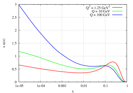
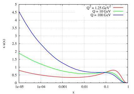
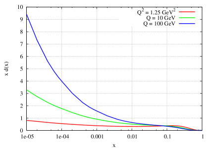
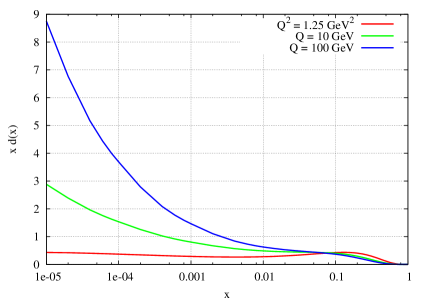
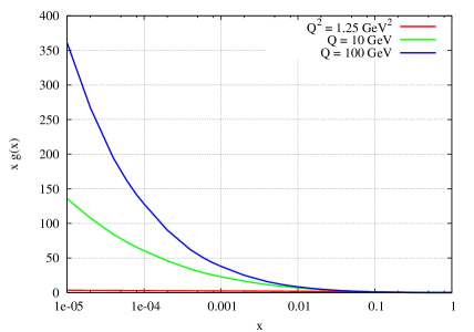
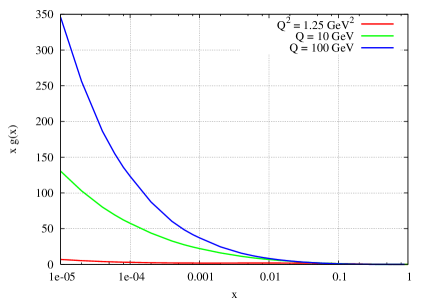
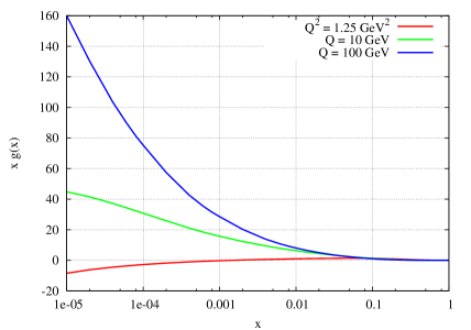
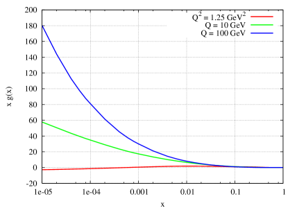
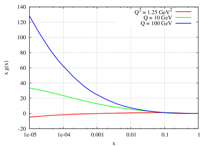
In Figg. (2.1 – 2.3), the evolution of up, down and gluon distributions at and in the unpolarized case is plotted at LO, NLO and NNLO. As initial distributions we have used both MRST and Alekhin distributions at the scale . Some details about the inputs are shown in the Table (2.1).
| MRST | Alekhin | |||||
| LO | NLO | NNLO | LO | NLO | NNLO | |
| file | lo2002.dat | alf119.dat | vnvalf1155.dat | a02m.pdfs_1_vfn | a02m.pdfs_2_vfn | a02m.pdfs_3_vfn |
| Ref. | [95] | [94] | [95] | [2] | [2] | [2] |
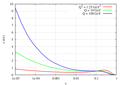
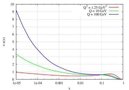
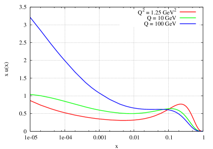
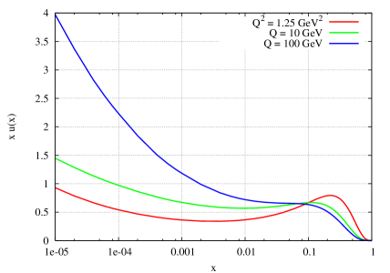
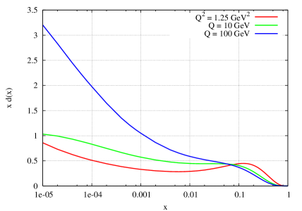
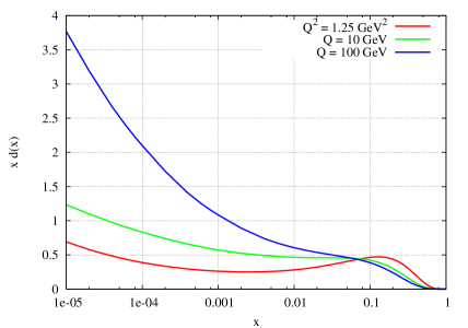
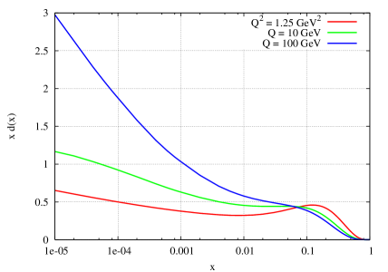
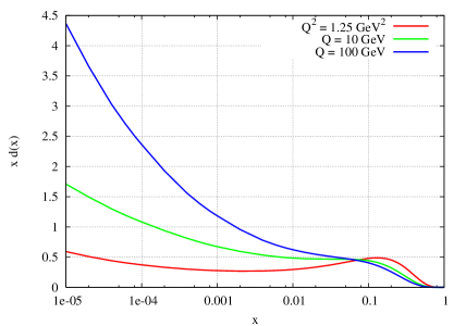

Chapter 3 NNLO precision studies of the Higgs total cross section
3.1 Introduction
One of the main objective at the LHC will be the search of the Higgs particle, which is responsible for the mechanism of mass generations for the fermions and the gauge bosons within the Standard Model. At the moment one of the most widely accepted ways to generate a mass for these particles relies on a scalar sector with a single Higgs field and a symmetry breaking potential. While the Lagrangian is invariant under a local symmetry of and this, of course, requires the same symmetry for the scalar sector as well, the vacuum of the theory, which is a stable state of minimum energy, doesn’t share the same symmetry. The presence of a minimal Higgs sector is also specific of the Standard Model, though many extensions of the Standard Model, supersymmetric and not, require a far more complex Higgs structure to give mass to both up-type and down-type quarks and to the leptons by some trilinear interactions termed Yukawa couplings. Our objective, in this chapter, is to present very accurate predictions for the total Higgs cross section by combining results available in the literature, specifically the computation of NNLO hard scatterings for the production of a scalar and a pseudoscalar Higgs in pp collisions. The analytical expressions are available through the work of Ravindran, Smith and van Neerven [107]. These have been combined with the NNLO evolution of the parton distributions in order to generate very accurate cross sections for the Higgs search at the LHC.
After the submission of this thesis, the preliminar work presented in this chapter has been completed and published in [31].
3.2 Higgs detection at hadron colliders
We summarize some generalities on the Standard Model and the mechanism of mass generation, with an emphasis on their phenomenological implications to hadron colliders.
The electroweak sector of the standard model is a chiral theory gauge theory containing gauge bosons, , and one gauge boson, . Left-handed and right-handed quarks couple differently to the 3 gauge bosons of the weak isospin and to . The Lagrangian is given by
| (3.1) |
where
| (3.2) |
A complex scalar field, doublet of is introduced and defined as
| (3.3) |
and with a scalar potential given by
| (3.4) |
(). This turns out to be the most general renormalizable and invariant potential allowed. The minimum of the potential is now a valley of equivalent vacua, among which we choose a vacuum by a suitable parameterization. One possibility is given by
| (3.5) |
with a hypercharge . The electromagnetic charge is and once can easily check that this state has not electric charge since
| (3.6) |
The vacuum expectation value of Eq. 3.5 allows to leave the intact by making one linear combination of the third component of and gauge symmetric, with identified with the generator of , according to the braking pattern
. The masses of the gauge bosons are generated by the kinetic part of the Higgs Lagrangian
| (3.7) |
where are the Pauli matrices. The explicit form of the covariant derivatives is
| (3.8) |
In unitary gauge the scalar field can be written as
| (3.9) |
and the contribution to the gauge boson masses from the scalar kinetic energy term are
| (3.10) |
To summarize, the masses of the massive gauge bosons
| (3.11) |
are given by
| (3.12) |
and the coupling constants satisfy relations
| (3.13) |
with being the Weinberg angle. Notice that in the unitary gauge a counting of the degrees of freedom for the Higgs scalar and the gauge bosons remains the same, as expected, without the appearance of unphysical Goldstone bosons. Alternative parameterizations, a la Kibble
| (3.14) |
let the Goldstone modes appear from the scalar sector. The appearance of this modes is a gauge variant effect. Non unitary gauges are important especially in the context of testing the unitarity of the model. In the Standard Model, there are three Goldstone bosons, , with masses and in the Feynman gauge.
In addition to giving the and bosons their masses, the Higgs boson is also responsible for giving the mass to the fermions. Thegauge invariant Yukawa coupling of the Higgs boson to fermions is given by trilinear terms of the form
| (3.15) |
where the left handed fermion doublet is constructed by acting with the chiral Lorenz projectors on both components
| (3.16) |
This gives the effective coupling
| (3.17) |
which can be seen to yield a mass term for the down quark if we make the identification
| (3.18) |
The mass term for the up quark is obtained by giving a value expectation value to the field which is an doublet and allows to write down the invariant coupling
| (3.19) |
which is the mass term for the up quark. For the upper components of the lepton doublets the procedure is the same, though the generation of a mass term for the neutrino is still a problem within the Standard Model. The neutrino appears only in its left-component and therefore has no Yukawa coupling.
For the multi-family case, the Yukawa couplings, and , become matrices which are valued in family space () with being the number of families. If we introduce a family mixing matrix and define and to be the and coupling constant the final Lagrangian describing the interactions of the leptons with the massive gauge bosons is
where
| (3.21) |
while for the quarks one obtains


A complete set of Feynman rules describing the interaction of the Higgs with the massive states of the Standard Model in both unitary and non unitary gauges, which involve the goldstones, can be found in [20]. The Higgs field, being responsible for the mechanism of mass generation, can be radiated off by any massive state and its coupling is proportional to the mass of the same state. At the LHC one of the golden plated modes to search for the Higgs is its production via the mechanism of gluon fusion. The leading order contribution is shown in fig. (3.1) which shows the dependence of the amplitude through the quark loop. Most of the contribution comes from the top quark, since this is the heaviest and has a larger coupling to the Higgs field. NLO and NNLO corrections have been computed in the last few years by various groups. A typical NLO correction is shown in fig. (3.2). From the computation of the LO diagram one gets
| (3.23) |
where and are color indices and p and q are the momenta of the two gluons. When the fermion in the loop is much heavier than the Higgs boson, the expression above becomes
| (3.24) |
which apparently does not depend on the quark mass. This implies that if there are additional generators, then the contribution of this process is proportional to the number of additional generations, providing an important window into new physics beyond the Standard Model. The resonant production of a heavy Higgs is instead given by the formula
| (3.25) |
relating the cross section for Higgs production via gluon fusion to the corresponding decay rate . At parton level we obtain
| (3.26) |
where is the energy in the gluon -gluon center of mass and the integral is defined by
| (3.27) |
3.2.1 The effective Lagrangian
An important feature of the result for Higgs boson production from gluon fusion is that it is independent of the heavy quark mass for a light Higgs boson. Eq. 3.24 can be derived from an effective vertex
with
| (3.28) |
being the contribution of heavy fermion loops to the QCD beta function. The effective Lagrangian can be used to compute the radiative corrections in the gluon sector. The correction in principle involve 2-loop diagrams. However, using the effective vertices from Eq. 3.2.1, the corrections can be found from a 1-loop calculation. In this way the contribution from the top quark loop is shrunk to a point. A discussion of the NNLO approach to the computation of the gluon fusion contributions to Higgs production has been presented in [107], work to which we refer for more details. We recall that in this work the authors present a study for both scalar and pseudoscalar Higgs production, the pseudoscalar appearing in 2-Higgs doublets models. In these extended models there is a mixing between the two scalars which is usually parameterized in terms of the ratio between the two vacuum expectation values at the minimum of the potential . Diagonalization of the mass matrix for the Higgs at the minimum introduces scalars and pseudoscalars interactions between the various Higgs and the quarks, as shown from the structure of the operator . Here we will briefly summarize their results.
In the large top-quark mass limit the Feynman rules for scalar Higgs production () can be derived from the effective Lagrangian density
| (3.29) |
whereas the production of a pseudo-scalar Higgs () is obtained from
| (3.30) |
where and represent the scalar and pseudo-scalar fields respectively and denotes the number of light flavours. is the field strength of QCD and the quark field are denoted by . With an appropriate normalization the constants turn out to be given by
| (3.31) |
and is defined by
| (3.32) |
where is the running coupling constant and denotes the renormalization scale. is the Fermi constant and the functions are given by
| (3.33) |
where denotes the mixing angle in the Two-Higgs-Doublet Model. Further and denote the masses of the (pseudo-) scalar Higgs boson and the top quark respectively. The coefficient functions originate from the corrections to the top-quark triangular graph provided one takes the limit . The coefficient functions are known up to order and are given by
| (3.34) | |||
| (3.35) |
where is given in the five-flavour number scheme.
Using the effective Lagrangian approach one can calculate the total cross section of the reaction
| (3.36) |
where and denote the incoming hadrons and represents an inclusive hadronic state. The total cross section is given by
| (3.37) |
where the factor is due to the average over colour and the parton distributions () depend on the mass factorization/renormalization scale . denotes the partonic hard scattering coefficient computed with NNLO accuracy.
3.3 Results
The use of our results on the NNLO evolution of the parton distributions together with the results of [107] allows us to provide accurate predictions for the total cross section for Higgs production. Here we summarize our numerical results which are illustrated in Figs. (3.3 – 3.6) and in Tables (3.1 – 3.4). The sets of distributions compared are those of MRST and Alekhin, currently the only ones available at NNLO. The plots refer to center of mass energies which are typical at the LHC, 14 TeV being the largest achievable in a not so distant future. The pseudoscalar cross section is systematically larger than the scalar one and both drop as the mass of the Higgs particles increases. The interval of variability which has been considered for this parameter is light-to-heavy (100 GeV to 300 GeV). The factorization scale and the renormalization scales have been chosen to coincide. For a given value of the Higgs mass, the cross section raises considerably with energy by a factor approximately 50-70 as we move from the lower toward the higher value of , the center of mass energy. Other distinct features of this study is the dependence of the result on the initial model chosen for the evolution. Finally the inclusion of the NNLO corrections, in all models, causes an increase in the actual values of the cross sections compared to the NLO results. A possible extension of this study is the inclusion of renormalization effects in the evolution and in the hard scatterings, which can be studied along the lines discussed in chapter 2.
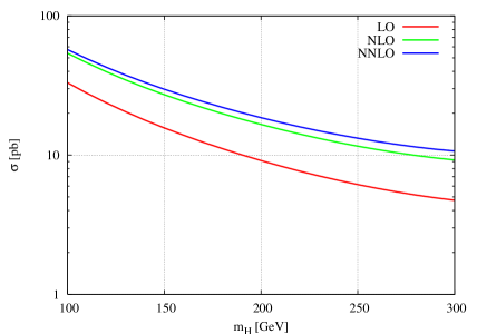
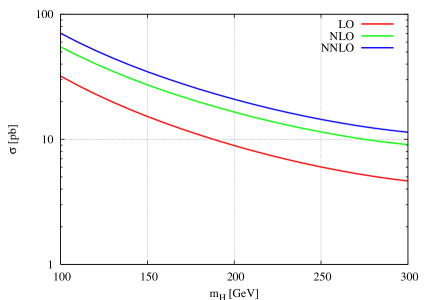
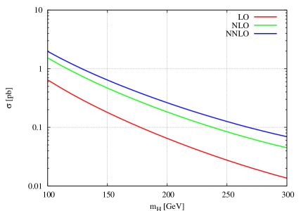
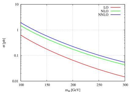
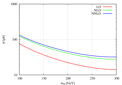
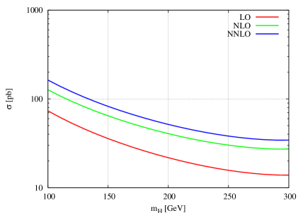
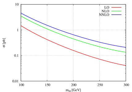
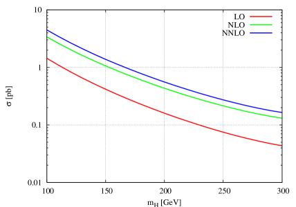
| LO | NLO | NNLO | ||||
|---|---|---|---|---|---|---|
| MRST | Alekhin | MRST | Alekhin | MRST | Alekhin | |
| LO | NLO | NNLO | ||||
|---|---|---|---|---|---|---|
| MRST | Alekhin | MRST | Alekhin | MRST | Alekhin | |
| LO | NLO | NNLO | ||||
|---|---|---|---|---|---|---|
| MRST | Alekhin | MRST | Alekhin | MRST | Alekhin | |
| LO | NLO | NNLO | ||||
|---|---|---|---|---|---|---|
| MRST | Alekhin | MRST | Alekhin | MRST | Alekhin | |
Chapter 4 The kinetic interpretation of the DGLAP Equation, its Kramers-Moyal
expansion and positivity of helicity distributions
4.1 Background on the topic
In this chapter and in the chapter that follows we elaborate on what has come to be known as the “kinetic description” of the dynamics of partons under the action of the renormalization group. In the DGLAP evolution the parton densities tend to be supported by smaller and smaller values of the Bjorken variable as the energy variable increases. Building on previous observations by Teryaev and by Collins and Qiu we clarify that the DGLAP evolution can be interpreted as a kinetic master equation which can be expanded formally to generate a hierarchy of new equations using the Kramers-Moyal approach. Arrested to the second order, this expansion generates a Fokker-Planck approximation to the DGLAP evolution. The issue of positivity of the kernels is important in order for this picture to hold. The LO kernels have this property, while at NLO a formal proof of positivity is more intricate and requires a numerical analysis to be supported. The hierarchy of equations generated by the Kramers-Moyal expansion could be studied independently, possibly numerically in order to gain more insight into the property of this expansion. One of the consequence of the kinetic interpretation, as shown in this chapter is the proof is that parton dynamics is reminscent of a “downward biased random walk”. These issues are analyzed in detail.
4.2 Introduction
According to a rederivation - due to Collins and Qiu - the DGLAP equation can be reinterpreted (in leading order) in a probabilistic way. This form of the equation has been used indirectly to prove the bound between polarized and unpolarized distributions, or positivity of the helicity distributions, for any . We reanalyze this issue by performing a detailed numerical study of the positivity bounds of the helicity distributions. We also elaborate on some of the formal properties of the Collins-Qiu form and comment on the underlying regularization, introduce a Kramers-Moyal expansion of the equation and briefly analyze its Fokker-Planck approximation. These follow quite naturally once the master version is given. We illustrate this expansion both for the valence quark distribution and for the transverse spin distribution and analyze the role of one well known inequality from this perspective. In fact, an interesting constraint relating longitudinally polarized, unpolarized and transversely polarized distributions is Soffer’s inequality, which deserves a special attention, since has to be respected by the evolution to any order in . Some tests of the inequality have been performed in the near past, bringing support to it. However, other inequalities are supposed to hold as well.
In this work we perform a NLO analysis of an inequality which relates longitudinally polarized distributions and unpolarized ones. The inequality can be summarized in the statement that helicity distributions (positive and negative) for quarks and gluons have to be positive. The inequality states that
| (4.1) |
or
| (4.2) |
where the refers to the the possible values of the helicities of quarks and gluons. The statement is supposed to hold, at least in leading order, for any . To analyze the renormalization group evolution of this relation, especially to next-to-leading order, requires some effort since this study involves a combined study of the (longitudinally) polarized and unpolarized evolutions. In this work we present a complete NLO study of the evolution equations starting directly from the helicity basis. Helicities are in fact the basic parton distributions from which other distributions can be built.
Compared to other implementations, in our work we perform a NLO test of the positivity of the helicity distributions using an ansatz due to Rossi [109] which reduces the evolution equations to an infinite set of recursion relations for some scale invariant coefficients.
Various arguments to validate eq. (4.2) have been presented in the literature. From our perspective, an interesting one has been formulated by Teryaev and Collaborators who have tried to establish a link, to leading order, between evolution equations and their probabilistic interpretation in order to prove Soffer’s inequality. Similar arguments hold also in the analysis of eq. (4.2).
We should remark that a complete probabilistic picture exists only for the leading order unpolarized evolution [38] and the arguments of [21] are inspired by the fact that the subtraction terms (the contributions in the expressions of the kernels, where is Bjorken’s variable), being positive, once they are combined with the bulk () contributions give a form of the evolution equations which are diagonal in parton type and resemble “kinetic” equations. Our arguments, on this issue, are just a refinement of this previous and influential analysis.
In the recent literature there has been some attention to this feature of the DGLAP evolution, limited to the nonsinglet sector, in connection with kinetic theory and the "dynamical renormalization group”, in the words of ref. [23].
All the arguments, so far, go back to some important older work of Collins and Qiu who provided an interesting derivation of the (unpolarized) DGLAP equation using Mueller’s formalism of cut diagrams. In their paper [38] the authors reinterpreted the DGLAP equation as a kinetic probabilistic equation of Boltzmann type. The authors gave no detail on some of the issues concerning the regularization of their diagrammatic expansion, on which we will elaborate since we need it for our accurate numerical analysis. In our work the Collins-Qiu form of the DGLAP equation is interpreted simply as a master equation rather than a Boltzmann equation, given the absence of a 2-to-2 scattering cross section in the probabilistic partonic interpretation. A master equation is governed by transition probabilities and various formal approximations find their way once this conceptual step is made. We illustrate, in the spirit of a stochastic approach to the DGLAP dynamics, how to extract standard differential equations of Kramers-Moyal type for the simplest nonsinglet evolutions, those involving valence distributions and transverse spin distributions.
We show that the DGLAP dynamics can be described, at least in a formal way, by a differential equation of arbitrarily high order. Truncations of this expansion to the first few orders provide the usual link with the Fokker-Planck approximation, the Langevin equation and its path integral version 111For an example of this interplay between differential and stochastic descriptions we refer the reader to [12]. The picture one should have in mind, at least in this approximation, is that of a stochastic (Brownian) dynamics of Bjorken’s variable in a fictitious time , describing the evolution under the renormalization group (RG). In this interpretation the probability function is the parton distribution itself.
This chapter is based on the paper [26].
4.3 Master Equations and Positivity
Let’s start considering a generic 1-D master equation for transition probabilities which we interpret as the probability of making a transition to a point given a starting point for a given physical system. The picture we have in mind is that of a gas of particles making collisions in 1-D and entering the interval with a probability per single transition, or leaving it with a transition probability . In general one writes down a master equation
| (4.3) |
describing the time evolution of the density of the gas undergoing collisions or the motion of a many replicas of walkers of density jumping with a pre-assigned probability, according to taste.
The result of Collins a Qiu, who were after a derivation of the DGLAP equation that could include automatically also the “edge point” contributions (or x=1 terms of the DGLAP kernels) is in pointing out the existence of a probabilistic picture of the DGLAP dynamics. These edge point terms had been always introduced in the past only by hand and serve to enforce the baryon number sum rule and the momentum sum rule as , the momentum scale, varies.
The kinetic interpretation was used in [21] to provide an alternative proof of Soffer’s inequality. We recall that this inequality
| (4.4) |
famous by now, sets a bound on the transverse spin distribution in terms of the components of the positive helicity component of the quarks, for a given flavour. The inequality has to be respected by the evolution. We recall that , also denoted by the symbol
| (4.5) |
has the property of being purely nonsinglet and of appearing at leading twist. It is identifiable in transversely polarized hadron-hadron collisions and not in Deep Inelastic Scattering (DIS), where can appear only through an insertion of the electron mass in the unitarity graph of DIS.
The connection between the Collins-Qiu form of the DGLAP equation and the master equation is established as follows. The DGLAP equation, in its original formulation is generically written as
| (4.6) |
where we are assuming a scalar form of the equation, such as in the nonsinglet sector. The generalization to the singlet sector of the arguments given below is, of course, quite straightforward. To arrive at a probabilistic picture of the equation we start reinterpreting as a time variable, while the parton density lives in a one dimensional (Bjorken) space.
We recall that the kernels are defined as “plus” distributions. Conservation of baryon number, for instance, is enforced by the addition of edge-point contributions proportional to .
We start with the following form of the kernel
| (4.7) |
where we have separated the edge point contributions from the rest of the kernel, here called . This manipulation is understood in all the equations that follow. The equation is rewritten in the following form
| (4.8) |
Now, if we define
| (4.9) |
(4.8) becomes a master equation for the probability function
| (4.10) |
There are some interesting features of this special master equation. Differently from other master equations, where transitions are allowed from a given x both toward and , in this case, transitions toward x take place only from values and leave the momentum cell only toward smaller y values (see Fig.(4.1).

Clearly, this sets a direction of the kinetic evolution of the densities from large x values toward smaller-x values as , the fictitious “time” variable, increases.
Probably this is the simplest illustration of the fact that parton densities, at large final evolution scales, are dominated by their small-x behaviour. As the “randomly moving partons” reach the region of momentum space, they find no space where to go, while other partons tend to pile up toward the same region from above. This is the picture of a random walk biased to move downward (toward the small-x region) and is illustrated in Fig. (4.1).
4.4 Probabilistic Kernels
We briefly discuss some salient features of the structure of the kernels in this approach and comment on the type of regularization involved in order to define them appropriately.
We recall that unpolarized and polarized kernels, in leading order, are given by
| (4.11) |
where
and
| (4.12) |
while the LO transverse kernels are given by
| (4.13) |
The unpolarized kernels should be compared with the Collins-Qiu form
where
These kernels need a suitable regularization to be well defined. Below we will analyze the implicit regularization underlying eq. (LABEL:cq1). One observation is however almost immediate: the component is not of the form given by eq. (4.7). In general, therefore, in the singlet case, the generalization of eq. (4.7) is given by
| (4.16) |
and a probabilistic interpretation is more complex compared to the nonsinglet case and has been discussed in the original literature [38].
4.5 Convolutions and Master Form of the Singlet
Distributions are folded with the kernels and the result rearranged in order to simplify the structure of the equations. Since in the previous literature this is done in a rather involute way [53] we provide here a simplification, from which the equivalence of the various forms of the kernel, in the various regularizations adopted, will be apparent. All we need is the simple relation
| (4.17) |
in which, on the right hand side, regularity of both the first and the second term is explicit. For instance, the evolution equations become
with . The same simplified form is obtained from the probabilistic version, having defined a suitable regularization of the edge point singularities in the integrals over the components in eq. (LABEL:cq2). The canonical expressions of the kernels (4.12), expressed in terms of “+” distributions, can also be rearranged to look like their equivalent probabilistic form by isolating the edge-point contributions hidden in their “+” distributions. We get the expressions
| (4.19) |
and
| (4.20) |
the other expressions remaining invariant. In appendix A we provide some technical details on the equivalence between the convolutions obtained using these kernels with the standard ones.
A master form of the singlet (unpolarized) equation is obtained by a straightforward change of variable in the decreasing terms. We obtain
| (4.21) | |||||
with a suitable (unique) cutoff needed to cast the equation in the form (LABEL:standard). A discussion of this aspect is left in appendix B. The (regulated) transition probabilities are then given by
as one can easily deduct from the form of eq. (4.10).
4.6 A Kramers-Moyal Expansion for the DGLAP Equation
Kramers-Moyal (KM) expansions of the master equations (backward or forward) are sometimes useful in order to gain insight into the master equation itself, since they may provide a complementary view of the underlying dynamics.
The expansion allows to get rid of the integral which characterizes the master equation, at the cost of introducing a differential operator of arbitrary order. For the approximation to be useful, one has to stop the expansion after the first few orders. In many cases this turns out to be possible. Examples of processes of this type are special Langevin processes and processes described by a Fokker-Planck operator. In these cases the probabilistic interpretation allows us to write down a fictitious Lagrangian, a corresponding path integral and solve for the propagators using the Feynman-Kac formula. For definitess we take the integral to cover all the real axis in the variable
| (4.23) |
As we will see below, in the DGLAP case some modifications to the usual form of the KM expansion will appear. At this point we perform a KM expansion of the equation in the usual way. We make the substitutions in the master equation in the first term and in the second term
| (4.24) |
identically equal to
| (4.25) |
with . First and second term in the equation above differ by a shift (in ) and can be related using a Taylor (or KM) expansion of the first term
| (4.26) |
where the term has canceled between the first and the second contribution coming from (4.25). The result can be written in the form
| (4.27) |
where
| (4.28) |
In the DGLAP case we need to amend the former derivation, due to the presence of boundaries in the Bjorken variable . For simplicity we will focus on the nonsinglet case. We rewrite the master equation using the same change of variables used above
| (4.29) | |||||
where we have introduced the simplest form of the Moyal product 222A note for noncommutative geometers: this simplified form is obtained for a dissipative dynamics when the p’s of phase space are replaced by constants. Here we have only one variable:
| (4.30) |
and . The expansion is of the form
| (4.31) |
which can be reduced to a differential equation of arbitrary order using simple manipulations. We recall that the Fokker-Planck approximation is obtained stopping the expansion at the second order
| (4.32) |
with
| (4.33) |
being moments of the transition probability function . Given the boundary conditions on the Bjorken variable x, even in the Fokker-Planck approximation, the Fokker-Planck version of the DGLAP equation is slightly more involved than Eq. (4.32) and the coefficients need to be redefined.
4.7 The Fokker-Planck Approximation
The probabilistic interpretation of the DGLAP equation motivates us to investigate the role of the Fokker-Planck (FP) approximation to the equation and its possible practical use. We should start by saying a word of caution regarding this expansion.
In the context of a random walk, an all-order derivative expansion of the master equation can be arrested to the first few terms either if the conditions of Pawula’s theorem are satisfied -in which case the FP approximation turns out to be exact- or if the transition probabilities show an exponential decay above a certain distance allowed to the random walk. Since the DGLAP kernels show only an algebraic decay in x, and there isn’t any explicit scale in the kernel themselves, the expansion is questionable. However, from a formal viewpoint, it is still allowed. With these caveats in mind we proceed to investigate the features of this expansion.
We redefine
| (4.34) |
For the first two terms one can easily work out the relations
| (4.35) | |||||
Let’s see what happens when we arrest the expansion (4.31) to the first 3 terms. The Fokker-Planck version of the equation is obtained by including in the approximation only with .
The Fokker-Planck limit of the (nonsinglet) equation is then given by
| (4.36) |
which we rewrite explicitly as
| (4.37) | |||||
A similar approach can be followed also for other cases, for which a probabilistic picture (a derivation of Collins-Qiu type) has not been established yet, such as for . We describe briefly how to proceed in this case.
First of all, we rewrite the evolution equation for the transversity in a suitable master form. This is possible since the subtraction terms can be written as integrals of a positive function. A possibility is to choose the transition probabilities
which reproduce the evolution equation for in master form
| (4.39) |
The Kramers-Moyal expansion is derived as before, with some slight modifications. The result is obtained introducing an intermediate cutoff which is removed at the end. In this case we get
Notice that compared to the standard Fokker-Planck approximation, the boundary now generates a term on the left-hand-side of the equation proportional to which is absent in eq. (4.32). This and higher order approximations to the DGLAP equation can be studied systematically both analytically and numerically and it is possible to assess the validity of the approximation [25].
4.8 Helicities to LO
As we have mentioned above, an interesting version of the usual DGLAP equation involves the helicity distributions.
We start introducing [21] the DGLAP kernels for fixed helicities and which will be used below. denotes (generically) the unpolarized kernels, while the are the longitudinally polarized ones. These definitions, throughout the chapter, are meant to be expanded up to NLO, the order at which our numerical analysis holds.

The equations, in the helicity basis, are
| (4.40) |
The nonsinglet (valence) analogue of this equation is also easy to write down
| (4.41) |
where the are the valence components of fixed helicities. The kernels in this basis are given by
| (4.42) |
Taking linear combinations of these equations (adding and subtracting), one recovers the usual evolutions for unpolarized and longitudinally polarized distributions. We recall that the unpolarized distributions, the polarized and the transversely polarized are related by

| (4.43) |
at any of the evolution and, in particular, at the boundary of the evolution.

Similar definition have been introduced for the gluon sector with denoting the fixed helicities of the gluon distributions with and being the corresponding longitudinal asymmetry and the unpolarized density respectively.

4.9 Summary of Positivity Arguments
Let us recapitulate here the basic arguments [21] that are brought forward in order to prove the positivity of the evolution to NLO.
If
| (4.44) |
then both kernels and are positive as far as .
The singular contributions at , which appear as subtraction terms in the evolution and which could, in principle, alter positivity, appear only in diagonal form, which means that they are only contained in , multiplied by the single functions or
| (4.45) |
| (4.46) |
| (4.47) |
Let’s focus just on the equation for (4.45). Rewriting the diagonal contribution as a master equation
| (4.48) |
in terms of a transition probability
| (4.49) |
which can be easily established to be positive, as we are going to show rigorously below, as far as all the remaining terms (the ellipses) are positive. We have performed a detailed numerical analysis to show the positivity of the contributions at .
This last condition is also clearly satisfied, since the contributions appear only in and are diagonal in the helicity of the various flavours (q, g). For a rigorous proof of the positivity of the solutions of master equations we proceed as follows.

Let be a positive distribution for and let us assume that it vanishes at , after which it turns negative. We also assume that the evolution of is of the form (4.7) with positive transition probabilities and . Notice that since the function is continuous together with its first derivative and decreasing, continuity of its first derivative will require at and in its neighbor. However, eq. (4.7) requires that at
| (4.50) |
which is positive, and we have a contradiction. We can picture the evolution in of these functions as a family of curves getting support to smaller and smaller x-values as grows and being almost vanishing at intermediate and large x values. We should mention that this proof does not require a complete probabilistic picture of the evolution, but just the positivity of the bulk part of the kernels, the positivity of the edge point subtractions and their diagonality in flavour. From Figs. (4.2) and (4.5) it is also evident that the leading order kernels are positive, together with the and (Fig. (4.3)) sectors.
The edge point contributions, generating the “subtraction terms” in the master equations for the “++” components of the kernels are positive, as is illustrated in 3 Tables included in Appendix A. There we have organized these terms in the form with
| (4.51) |
with A and B being numerical coefficients depending on the number of flavours included in the kernels. Notice that the subtraction terms are always of the form (4.51), with the (diverging) logarithmic contribution () regulated by a cutoff. This divergence in the convolution cancels when these terms are combined with the divergence at of the first term of the master equation for all the relevant components containing “+” distributions. It is crucial, however, to establish positivity of the evolution of the helicities that the boundary conditions on the evolution be satisfied. Initial conditions have this special property, in most of models, and the proof of positivity of all the distributions therefore holds at any .
As we move to NLO, the pattern gets more complicated. In fact, from a numerical check, one can see that some NLO kernels turn to be negative, including the unpolarized kernels and the helicity kernels, while others (Fig. (4.4)) are positive. One can also notice the presence of a crossing of several helicity components in the and sectors (see Fig. (4.7)) at larger x values, while in the small-x region some components turn negative (Fig. (4.6)). There is no compelling proof of positivity, in this case, either than that coming from a direct numerical analysis.

We have seen that master forms of evolution equations, for evolutions of all kinds, when found, can be used to establish positivity of the evolution itself.
The requirements have been spelled out above and can be summarized in the following points: 1) diagonality of the decreasing terms, 2) initial positivity of the distributions, 3) positivity of the remaining (non diagonal) kernels. As we have also seen, some of these conditions are not satisfied by the NLO evolution.
4.10 Results
In regard to the input distributions we used, we refer the reader to Sec. 1.8.
We show in Fig. 4.8 results for the evolution of the distribution at the initial scale ( GeV) and at two final scales, 100 GeV and 200 GeV respectively. The peaks at the various scales get lowered and become more pronounced toward the smaller x region as Q increases. In Fig. 4.9 show an apparent steeper growth at small-x compared to . For the distributions the situation is inverted, with growing steeper compared to (Figs. 4.11 and 4.12 respectively). This apparent behaviour is resolved in Figs. (4.10) and (4.13) from which it is evident that both plus and minus components converge, at very small-x values, toward the same limit.
The components s,c,t and b (Figs. 4.14-4.21) have been generated radiatively from vanishing initial conditions for final evolution scales of 100 and 200 GeV and 200 GeV (t).
Both positive and negative components grow steadily at small-x and are negligible at larger x values. The distribution for the top quark has been included for completeness. Given the smaller evolution interval the helicity distributions for heavier generations are suppressed compared to those of lighter flavours. Gluon helicities (Figs. 4.22, 4.23) are also enhanced at small-x, and show a similar growth. The fine difference between the quark u and d distributions are shown in Figs. 4.10 and 4.13.
Finally in Figs. 4.24, 4.25 and 4.26 we plot simultaneously longitudinally polarized, unpolarized and helicity distributions for up quarks, down quarks and gluons at an intermediate factorization scale of 100 GeV, relevant for experiments at RHIC. Notice that while and are positive and their difference is also positive, for down quarks the two helicity components are positive while their difference is negative. Gluons, in the model studied here, have a positive longitudinal polarization, and their helicity components are also positive. The positive and negative gluon helicities are plotted in two separate figures, Figs. 4.22 and 4.23, while their difference, is shown in Fig. 4.27. One can observe, at least in this model, a crossing at small-x in this distribution.
We conclude that, at least for this set of boundary conditions, positivity of all the components holds to NLO, as expected.
We also report three tables (4.1 – 4.3) illustrating the (positive) numerical values of the contributions coming from the subtraction terms in the NLO kernels. Coefficients and refer to the subtraction terms as explained in the section above.
| 3 | 12.5302 | 12.1739 |
|---|---|---|
| 4 | 10.9569 | 10.6924 |
| 5 | 9.3836 | 9.2109 |
| 6 | 7.8103 | 7.7249 |
| 3 | 12.5302 | 12.1739 |
|---|---|---|
| 4 | 10.9569 | 10.6924 |
| 5 | 9.3836 | 9.2109 |
| 6 | 7.8103 | 7.7249 |
| 3 | 48.4555 | 27.3912 |
|---|---|---|
| 4 | 45.7889 | 24.0579 |
| 5 | 43.1222 | 20.7245 |
| 6 | 40.4555 | 17.3912 |
4.11 Regularizations
The “+” plus form of the kernels and all the other forms introduced before, obtained by separating the contributions from the edge-point from those coming from the bulk are all equivalent, as we are going to show, with the understanding that a linear (unique) cutoff is used to regulate the divergences both at x=0 and at x=1. We focus here on the two possible sources of singularity, i.e. on and on the contributions, which require some attention. Let’s start from the case. We recall that “+” plus distributions are defined as
| (4.52) |
with being a cutoff for the edge-point contribution.
We will be using the relations
| (4.53) |
Using the expressions above it is easy to obtain
which is eq. (4.17). If we remove the “+” distributions and adopt (implicitly) a cutoff regularization, we need special care. In the probabilistic version of the kernel, the handling of is rather straightforward
and using eqs. (4.53) we easily obtain
| (4.56) | |||||
Now consider the convolution in the Collins-Qiu form. We get
| (4.57) | |||||
There are some terms in the expression above that require some care. The appropriate regularization is
| (4.58) |
Observe also that
| (4.59) |
Notice that in this regularization the singularity of at is traded for a singularity at z=1 in . It is then rather straightforward to show that
| (4.60) | |||||
A final comment is due for the form of the sum rule
| (4.61) |
that we need to check with the regularization given above.
The strategy to handle this expression is the same as before. We extract all the and integration terms and use
to eliminate the singularities at the boundaries and verify eq. (4.61).


4.12 Conclusions
We have discussed in detail some of the main features of the probabilistic approach to the DGLAP evolution in the helicity basis. Numerical results for the evolution of all the helicities have been provided, using a special algorithm, based in -space. We have also illustrated some of the essential differences between the standard distributional form of the kernels and their probabilistic version, clarifying some issues connected to their regularization. Then we have turned to the probabilistic picture, stressing on the connection between the random walk approach to parton diffusion in -space and the master form of the DGLAP equation. The link between the two descriptions has been discussed especially in the context of the Kramers-Moyal expansion. A Fokker-Planck approximation to the expansion has also been presented which may turn useful for the study of formal properties of the probabilistic evolution. We have also seen that positivity of the helicity distributions, to NLO, requires a numerical analysis, as already hinted in [21]. Our study also validates the use of a very fast evolution algorithm, alternative to other standard algorithms based on Mellin algorithms, whose advantage is especially in the analysis of the evolution of nonforward parton distributions, as we will show elsewhere.
Chapter 5 An -space analysis of evolution equations: Soffer’s inequality and the
nonforward evolution
We analyze the use of algorithms based in -space for the solution of renormalization group equations of DGLAP-type and test their consistency by studying bounds among partons distributions - in our specific case Soffer’s inequality and the perturbative behaviour of the nucleon tensor charge - to next-to-leading order in QCD.
We also comment on the (kinetic) proof of positivity of the evolution of , using a kinetic analogy, along the lines of the previous chapter, and illustrate the extension of the algorithm to the evolution of generalized parton distributions. We prove positivity of the nonforward evolution in a special case and illustrate a Fokker-Planck approximation to it.
5.1 Introduction
One of the most fascinating aspects of the structure of the nucleon is the study of the distribution of spin among its constituents, a topic of remarkable conceptual complexity which has gained a lot of attention in recent years. This study is entirely based on the classification and on the phenomenological modeling of all the leading-twist parton distributions, used as building blocks for further investigations in hadronic physics.
There are various theoretical ways to gather information on these non-local matrix elements. One among the various possibilities is to discover sum rules connecting moments of these distributions to other fundamental observables. Another possibility is to discover bounds - or inequalities - among them and use these results in the process of their modeling. There are various bounds that can be studied, particularly in the context of the new generalized parton dynamics typical of the skewed distributions [82, 106]. All these relations can be analyzed in perturbation theory and studied using the Renormalization Group (RG), although a complete description of their perturbative dynamics is still missing. This study, we believe, may require considerable theoretical effort since it involves a global understanding both of the (older) forward (DGLAP) dynamics and of the generalized new dynamics encoded in the skewed distributions.
In this context, a program aimed at the study of various bounds in perturbation theory using primarily a parton dynamics in -space has been outlined [25]. This requires accurate algorithms to solve the equations up to next-to-leading order (NLO). Also, underlying this type of description is, in many cases, a probabilistic approach [22] which has some interesting consequences worth of a closer look . In fact, the DGLAP equation, viewed as a probabilistic process, can be rewritten in a master form which is at the root of some interesting formal developments. In particular, a wide set of results, available from the theory of stochastic processes, find their way in the study of the evolution. We have elaborated on this issue in previous work [25] and proposed a Kramers-Moyal expansion of the DGLAP equation as an alternative way to describe its dynamics. Here, this analysis will be extended to the case of the nonforward evolution.
With these objectives in mind, in this study we test -space algorithms up to NLO and verify their accuracy using a stringent test: Soffer’s inequality. As usual, we are bound to work with specific models of initial conditions. The implementations on which our analysis are based are general, with a varying flavour number at any threshold of intermediate quark mass in the evolution. Here, we address Soffer’s inequality using an approach based on the notion of “superdistributions” [21], which are constructs designed to have a simple (positive) evolution thanks to the existence of an underlying master form [22, 25]. The original motivation for using such a master form (also termed kinetic or probabilistic) to prove positivity has been presented in [21], while further extensions of these arguments have been presented in [25]. In a final section we propose the extension of the evolution algorithm to the case of the skewed distributions, and illustrate its implementation in the nonsinglet case. As for the forward case, numerical tests of the inequality are performed for two different models. We show that even starting from a saturated inequality at the lowest evolution scale, the various models differ significantly even for a moderate final factorization scale of GeV. Finally, we illustrate in another application the evolution of the tensor charge and show that, in the models considered, differences in the prediction of the tensor charge are large.
5.2 Prelude to -space: A Simple Proof of Positivity of to NLO
There are some nice features of the parton dynamics, at least in the leading logarithmic approximation (LO), when viewed in -space, once a suitable “master form” of the parton evolution equations is identified.
The existence of such a master form, as firstly shown by Teryaev, is a special feature of the evolution equation itself. The topic has been addressed before in LO [21] and reanalyzed in more detail in [25] where, starting from a kinetic interpretation of the evolution, a differential equation obtained from the Kramers-Moyal expansion of the DGLAP equation has also been proposed.
The arguments of refs. [21, 25] are built around a form of the evolution equation which has a simple kinetic interpretation and is written in terms of transition probabilities constructed from the kernels.
The strategy used, at least in leading order, to demonstrate the positivity of the LO evolution for special combinations of parton distributions [21], to be defined below, or the NLO evolution for , which we are going to address, is based on some results of ref.[21], briefly reviewed here, in order to be self-contained.
A master equation is typically given by
| (5.1) |
and if through some manipulations, a DGLAP equation
| (5.2) |
with kernels , is rewritten in such a way to resemble eq. (5.1)
| (5.3) |
with a (positive) transition probability
| (5.4) |
then positivity of the evolution is established.
For equations of nonsinglet type, such as those evolving , the valence quark distribution, or , the transverse spin distribution, this rewriting of the equation is possible, at least in LO. NLO proofs are, in general, impossible to construct by this method, since the kernels turn out, in many cases, to be negative. The only possible proof, in these cases, is just a numerical one, for suitable (positive) boundary conditions observed by the initial form of the parton distributions. Positivity of the evolution is then a result of a non obvious interplay between the various contributions to the kernels in various regions in -space.
In order to discuss the probabilistic version of the DGLAP equation it is convenient to separate the bulk contributions of the kernels from the edge point contributions at . For this purpose we recall that the structure of the kernels is, in general, given by
| (5.5) |
where the bulk contributions and the edge point contributions have been explicitly separated. We focus on the transverse spin distributions as an example. With these prerequisites, proving the LO and NLO positivity of the transverse spin distributions is quite straightforward, but requires a numerical inspection of the transverse kernels. Since the evolutions for are purely nonsinglet, diagonality in flavour of the subtraction terms is satisfied, while the edge-point subtractions can be tested to be positive numerically. We illustrate the explicit construction of the master equation for in LO, since extensions to NLO of this construction are rather straightforward.
In this case the LO kernel is given by
| (5.6) |
and by some simple manipulations we can rewrite the corresponding evolution equation in a suitable master form. That this is possible is an elementary fact since the subtraction terms can be written as integrals of a positive function. For instance, a possibility is to choose the transition probabilities
which reproduce the evolution equation for in master form
| (5.8) |
The NLO proof of positivity is also rather straightforward. For this purpose we have analyzed numerically the behaviour of the NLO kernels both in their bulk region and at the edge-point. We show in Table 1 of Appendix B results for the edge point contributions to NLO for both of the components, which are numerically the same. There we have organized these terms in the form with
| (5.9) |
with A and B being numerical coefficients depending on the number of flavours included in the kernels. The (diverging) logarithmic contribution () have been regulated by a cutoff. This divergence in the convolution cancels when these terms are combined with the divergence at of the first term of the master equation (5.8) for all the relevant components containing “+” distributions. As for the bulk contributions , positivity up to NLO of the transverse kernels is shown numerically in Fig. (5.1). All the conditions of positivity are therefore satisfied and therefore the distributions evolve positively up to NLO. The existence of a master form of the equation is then guaranteed.
Notice that the NLO positivity of implies positivity of the nucleon tensor charge [81]
| (5.10) |
for each separate flavour for positive initial conditions. As we have just shown, this proof of positivity is very short, as far as one can check numerically that both components of eq.(5.8) are positive.
| 3 | 12.5302 | 12.1739 |
|---|---|---|
| 4 | 10.9569 | 10.6924 |
| 5 | 9.3836 | 9.2109 |
| 6 | 7.8103 | 7.7249 |
5.3 Soffer’s inequality
Numerical tests of Soffer’s inequality can be performed either in moment space or, as we are going to illustrate in the next section, directly in -space, using suitable algorithms to capture the perturbative nature of the evolution. We recall that Soffer’s inequality
| (5.11) |
sets a bound on the transverse spin distribution in terms of the components of the positive helicity component of the quarks, for a given flavour. An original proof of Soffer’s inequality in LO has been discussed in ref.[14], while in [21] an alternative proof was presented, based on a kinetic interpretation of the evolution equations.
We recall that , also denoted by the symbol
| (5.12) |
has the property of being purely nonsinglet and of appearing at leading twist. It is identifiable in transversely polarized hadron-hadron collisions and not in Deep Inelastic Scattering (from now on we will omit sometimes the -dependence in the kernels and in the distributions when obvious). In the following we will use interchangeably the notations and to denote the transverse asymmetries. We introduce also the combinations
where we sum over the flavor index , and we have introduced singlet and nonsinglet contributions for distributions of fixed helicities
In our analysis we solve all the equations in the helicity basis and reconstruct the various helicities after separating singlet and nonsinglet sectors. We mention that the nonsinglet sector is now given by a set of 2 equations, each involving helicities and the singlet sector is given by a 4-by-4 matrix.
In the singlet sector we have
| (5.15) |
while the nonsinglet (valence) analogue of this equation is also easy to write down
| (5.16) |
Above, is the flavor index, indicate components and the lower subscript stands for the helicity.
Similarly to the unpolarized case the flavour reconstruction is done by adding two additional equations for each flavour in the helicity
| (5.17) |
whose evolution is given by
The reconstruction of the various contributions in flavour space for the two helicities is finally done using the linear combinations
| (5.19) |
We will be needing these equations below when we present a proof of positivity up to LO, and we will thereafter proceed with a NLO implementation of these and other evolution equations. For this we will be needing some more notations.
We recall that the following relations are also true to all orders
between polarized and unpolarized kernels and
| (5.20) |
relating unpolarized kernels to longitudinally polarized ones. Generically, the kernels of various type are expanded up to NLO as
| (5.21) |
and specifically, in the transverse case we have
| (5.22) |
with the corresponding evolution equations
| (5.24) |
We also recall that the kernels in the helicity basis in LO are given by
| (5.25) |
An inequality, such as Soffer’s inequality, can be stated as positivity condition for suitable linear combinations of parton distributions [21] and this condition can be analyzed - as we have just shown for the case - in a most direct way using the master form.
For this purpose consider the linear valence combinations
which are termed “superdistributions” in ref.[21]. Notice that a proof of positivity of the distributions is equivalent to verify Soffer’s inequality. However, given the mixing of singlet and nonsinglet sectors, the analysis of the master form is, in this case, more complex. As we have just mentioned, what can spoil the proof of positivity, in general, is the negativity of the kernels to higher order. We anticipate here the result that we will illustrate below where we show that a LO proof of the positivity of the evolution for can be established using kinetic arguments, being the kernels are positive at this order. However we find that the NLO kernels do not satisfy this condition. In any case, let’s see how the identification of such master form proceeds in general. We find useful to illustrate the result using the separation between singlet and nonsinglet sectors. In this case we introduce the combinations
with .
Differentiating these two linear combinations (LABEL:separation) we get
which can be rewritten as
with being the nonsinglet (NS) kernel.
At this point we define the linear combinations
| (5.30) |
and rewrite the equations above as
where we have reintroduced as a flavour index. From this form of the equations it is easy to establish the leading order positivity of the evolution, after checking the positivity of the kernel and the existence of a master form.

The second nonsinglet sector is defined via the variables
| (5.32) |
which evolve as nonsinglets and the two additional distributions
| (5.33) |
Also in this case we introduce the kernels
| (5.34) |
to obtain the evolutions
For the singlet sector, we simply define , and the corresponding evolution is similar to the singlet equation of the helicity basis. Using the equations above, the distributions are then reconstructed as
| (5.36) |
and result positive for any flavour if the addends are positive as well. However, as we have just mentioned, positivity of all the kernels introduced above is easy to check numerically to LO, together with their diagonality in flavour which guarantees the existence of a master form.
As an example, consider the LO evolution of . The proof of positivity is a simple consequence of the structure of eq. (LABEL:pos1). In fact the edge-point contributions appear only in , i.e. they are diagonal in the evolution of . The inhomogeneous terms on the right hand side of (LABEL:pos1), proportional to are are harmless, since the kernel has no edge-point contributions. Therefore under 1) diagonality in flavour of the subtraction terms and 2) positivity of first and second term (transition probabilities) we can have positivity of the evolution. A refined arguments to support this claim has been presented in [25].
This construction is not valid to NLO. In fact, while the features of flavour diagonality of the master equation are satisfied, the transition probabilities are not positive in the whole range. The existence of a crossing from positive to negative values in can, in fact, be established quite easily using a numerical analysis. We illustrate in Figs. (5.2) and (5.3) plots of the kernels at LO and NLO, showing that, at NLO, the requirement of positivity of some components is violated. The limitations of this sort of proofs -based on kinetic arguments- are strictly linked to the positivity of the transition probabilities once a master form of the equation is identified.
5.4 An -space Expansion
We have seen that NLO proofs of positivity, can be -at least partially- obtained only for suitable sets of boundary conditions. To this purpose, we choose to investigate the numerical behaviour of the solution using -space based algorithms which need to be tested up to NLO.


Our study validates a method which can be used to solve evolution equations with accuracy in leading and in next-to-leading order. The method is entirely based on an expansion [109] used in the context of spin physics [75] and in supersymmetry [39]. An interesting feature of the expansion, once combined with Soffer’s inequality, is to generate an infinite set of relations among the scale invariant coefficients which characterize it.
In this approach, the NLO expansion of the distributions in the DGLAP equation is generically given by
| (5.37) |
where, to simplify the notation, we assume a short-hand matrix notation for all the convolution products. Therefore stands for a vector having as components any of the helicities of the various flavours .
If we introduce Rossi’s expansion for , , and the linear combinations (in short form)
we easily get the inequalities
| (5.39) |
and
| (5.40) |
valid to leading order,which we can check numerically. Notice that the signature factor has to be included due to the alternation in sign of the expansion. To next to leading order we obtain
| (5.41) | |||||
valid for , obtained after identification of the corresponding logarithmic powers at any . In general, one can assume a saturation of the inequality at the initial evolution scale
| (5.42) |
This initial condition has been evolved in solving the equations for the distributions to NLO.
5.5 Nonforward Extensions
In this section we finally discuss the nonforward extension of the evolution algorithm. In the case of nonforward distributions a second scaling parameter controls the asymmetry between the initial and the final nucleon momentum in the deeply virtual limit of nucleon Compton scattering. The solution of the evolution equations, in this case, are known in operatorial form. Single and double parton distributions are obtained sandwiching the operatorial solution with 4 possible types of initial/final states , corresponding, respectively, to the case of diagonal parton distributions, distribution amplitudes and, in the latter case, skewed and double parton distributions [106]. Here we will simply analyze the nonsinglet case and discuss the extension of the forward algorithm to this more general case. Therefore, given the off-forward distributions , in Ji’s notation, we set up the expansion
| (5.43) |
which is the natural extension of the forward algorithm discussed in the previous sections. We recall that in the light-cone gauge is defined as
| (5.44) |
with , [82] (symmetric choice) and .
This distribution describes for and the DGLAP-type region for the quark and the antiquark distribution respectively, and the ERBL [52] (see also [44] for an overview) distribution amplitude for . In the following we will omit the dependence from .
Again, once we insert the ansatz (5.43) into the evolution equations we obtain an infinite set of recursion relations which we can solve numerically. In LO, it is rather simple to relate the Gegenbauer moments of the skewed distributions and those of the generalized scaling coefficients . We recall that in the nonforward evolution, the multiplicatively renormalizable operators appearing in the light cone expansion are given in terms of Gegenbauer polynomials [106]. The Gegenbauer moments of the coefficients of our expansion (5.43) can be easily related to those of the off-forward distribution
| (5.45) |
The evolution of these moments is rather simple
| (5.46) |
with
| (5.47) |
being the nonsinglet anomalous dimensions. If we define the Gegenbauer moments of our expansion
| (5.48) |
we can relate the moments of the two expansions as
| (5.49) |
Notice that expansions similar to (5.43) hold also for other choices of kinematical variables, such as those defining the nonforward distributions [106], where the t-channel longitudinal momentum exchange is related to the longitudinal momentum of the incoming nucleon as . We recall that as defined in [82] can be mapped into two independent distributions and through the mappings [72]
in which the interval is split into two coverings, partially overlapping (for , or ERBL region) in terms of the two variables () and (). In this new parameterization, the momentum fraction carried by the emitted quark is , as in the case of ordinary distributions, where it is parametrized by Bjorken . For definitess, we focus here on the DGLAP-like region of the nonsinglet evolution. The nonsinglet kernel is given in this case by
| (5.51) |
we introduce a LO ansatz
| (5.52) |
and insert it into the evolution of this region to obtain the very simple recursion relations
| (5.53) | |||||
The recursion relations can be easily reduced to a weighted sum of contributions in which is a spectator parameter. Here we will not make a complete implementation, but we will illustrate in an appendix the general strategy to be followed. There we show a very accurate analytical method to evaluate the logarithms generated by the expansion without having to rely on brute-force computations.
5.6 Positivity of the nonsinglet Evolution
Positivity of the nonsinglet evolution is a simple consequence of the master-form associated to the nonforward kernel (5.51). As we have already emphasized above, positivity of the initial conditions are sufficient to guarantee a positivity of the solution at any scale . The master-form of the equation allows to reinterpret the parton dynamics as a random walk biased toward small-x values as increases.
In the nonforward case the identification of a transition probability for the random walk [25] associated with the evolution of the parton distribution is obtained via the nonforward transition probability
| (5.54) |
and the corresponding master equation is given by
| (5.55) |
that can be re-expressed in a form which is a simple generalization of the formula for the forward evolution [25].
| (5.56) | |||||
where a Moyal-like product appears
| (5.57) |
and . A Kramers-Moyal expansion of the equation allows to generate a differential equation of infinite order with a parametric dependence on
| (5.58) | |||||
We define
| (5.59) |
If we arrest the expansion at the first two terms we are able to derive an approximate equation describing the dynamics of partons for non-diagonal transitions. The procedure is a slight generalization of the method presented in [25], to which we refer for further details. For this purpose we use the identities
| (5.60) | |||||
which allow to compute the first few coefficients of the expansion. Using these relations, the Fokker-Planck approximation to this equation can be worked out explicitly. We omit details on the derivation which is non obvious since particular care is needed to regulate the (canceling) divergences and just quote the result.
A lengthy computation gives
where we have defined
| (5.62) |
This equation and all the equations obtained by arresting the Kramers-Moyal expansion to higher order provide a complementary description of the nonforward dynamics in the DGLAP region, at least in the nonsinglet case. Moving to higher order is straightforward although the results are slightly lengthier. A full-fledged study of these equations is under way and we expect that the DGLAP dynamics is reobtained - directly from these equations - as the order of the approximation increases.
5.7 Model comparisons, saturation and the tensor charge
In this last section we discuss some implementations of our methods to the standard (forward) evolution by doing a NLO model comparisons both in the analysis of Soffer’s inequality and for the evolution of the tensor charge. We have selected two models, motivated quite independently and we have compared the predicted evolution of the Soffer bound at an accessable final evolution scale around GeV for the light quarks and around GeV for the heavier generations. At this point we recall that in order to generate suitable initial conditions for the analysis of Soffer’s inequality, one needs an ansatz in order to quantify the difference between its left-hand side and right-hand side at its initial value.
The well known strategy to build reasonable initial conditions for the transverse spin distribution consists in generating polarized distributions (starting from the unpolarized ones) and then saturate the inequality at some lowest scale, which is the approach we have followed for all the models that we have implemented.
The first model we have used is the GRV-GRSV, that we have described in Sec. 1.8.
In the implementation of the second model (GGR model) we have used as input distributions in the unpolarized case the CTEQ4 parametrization [92], calculated to NLO in the scheme at a scale
| (5.63) |
and for and we have related the unpolarized input distribution to the longitudinally polarized ones by the relations [73]
| (5.64) |
and for .
A so-called “spin dilution factor” as defined in [73], which appears in the equations above is given by
| (5.65) |
In this second (GGR) model, in regard to the initial conditions for the gluons, we have made use of two different options, characterized by a parameter dependent on the corresponding option. The first option, that we will denote by GGR1, assumes that gluons are moderately polarized
| (5.66) |
while the second option (GGR2) assumes that gluons are not polarized
| (5.67) |
We have plotted both ratios and differences for various flavours as a function of . For the up quark, while the two models GGR1 and GGR2 are practically overlapping, the difference between the GGR and the GRSV models in the the ratio is only slightly remarked in the intermediate x region . In any case, it is just at the few percent level (Fig. (5.6)), while the inequality is satisfied with a ratio between the plus helicity distribution and transverse around 10 percent from the saturation value, and above. There is a wider gap in the inequality at small x, region characterized by larger transverse distribution, with values up to 40 percent from saturation. A similar trend is noticed for the x-behaviour of the inequality in the case of the down quark (Fig. 5.7). In this latter case the GGR and the GRSV model show a more remarked difference, especially for intermediate x-values. An interesting features appears in the corresponding plot for the strange quark (Fig.(5.8)), showing a much wider gap in the inequality (50 percent and higher) compared to the other quarks. Here we have plotted results for the two GGR models (GGR1 and GGR2). Differently from the case of the other quarks, in this case we observe a wider gap between lhs and rhs at larger x values, increasing as . In figs. (5.9)and (5.10) we plot the differences for strange and charm and for bottom and top quarks respectively, which show a much more reduced evolution from the saturation value up to the final corresponding evolving scales (100 and 200 GeV). As a final application we finally discuss the behaviour of the tensor charge of the up quark for the two models as a function of the final evolution scale . We recall that like the isoscalar and the isovector axial vector charges defined from the forward matrix element of the nucleon, the nucleon tensor charge is defined from the matrix element of the tensor current
| (5.68) |
where denotes the flavour (a) contribution to the nucleon tensor charge at a scale and is the transverse spin.
In fig. (5.11) we plot the evolution of the tensor charge for the models we have taken in exam. At the lowest evolution scales the charge is, in these models, above 1 and decreases slightly as the factorization scale increases. We have performed an evolution up to 200 GeV as an illustration of this behaviour. There are substantial differences between these models, as one can easily observe, which are around 20 percent. From the analysis of these differences at various factorization scales we can connect low energy dynamics to observables at higher energy, thereby distinguishing between the various models. Inclusion of the correct evolution, up to subleading order is, in general, essential.
5.8 Conclusions
We have illustrated the use of -space based algorithms for the solution of evolution equations in the leading and in the next-to-leading approximation and we have provided some applications of the method both in the analysis of Soffer’s inequality and in the investigation of other relations, such as the evolution of the proton tensor charge, for various models. The evolution has been implemented using a suitable base, relevant for an analysis of positivity in LO, using kinetic arguments. The same kinetic argument has been used to prove the positivity of the evolution of and of the tensor charge up to NLO. In our implementations we have completely relied on recursion relations without any reference to Mellin moments. We have provided several illustrations of the recursive algorithm and extended it to the nonforward evolution up to NLO. Building on previous work for the forward evolution, we have presented a master-form of the nonsinglet evolution of the skewed distributions, a simple proof of positivity and a related Kramers Moyal expansion, valid in the DGLAP region of the skewed evolution for any value of the asymmetry parameter . We hope to return with a complete study of the nonforward evolution and related issues not discussed here in the near future.


Chapter 6 Simulation of air showers: lateral distributions, multiplicities
and the
search for new physics at Auger
6.1 A brief overview
The inclusive high energy cosmic rays spectrum has been the focus point of a lot of attention in the last few years. The spectrum, at a first look, appears to be deprived of any structure and, on the other hand, drops dramatically as we move upward in energy. The region which we are interested in, in our study, is the high energy region, where a correct description of the underlying quark-gluon dynamics is important in order to gain some insight into the physics of the extensive air showers that form when a high energy primary (say a proton or a neutrino) collides with the nuclei in the atmosphere. Here we would like to put things into place in order to set up the stage for our analysis, which will be developed in this chapter and will be specialized in the next chapter to the case of mini black hole production in cosmic rays in the context of brane models. Our journey has been guided by our interest in applying standard QCD tools, such as the RG evolution of fragmentation functions, to this challenging environment. It turns out, as expected, that the issues to be analyzed, using the parton model, are manifold and do not have a clear-cut answer at the moment, although there is a general agreement that models based on reggeon theory, popular in the sixties, can capture the complex dynamics of a proton-air collision at those energies. The upper end of the cosmic rays spectrum (these cosmic rays are classified as ultra high energy cosmic rays or UHECR), in particular, has been affected by a controversy which has spanned several decades over the existence of a cutoff which would more or less sharply limit it to stay below eV.
In this chapter we perform large scale air shower simulations around the GZK cutoff are performed. An extensive analysis of the behaviour of the various subcomponents of the cascade is presented. We focus our investigation both on the study of total and partial multiplicities along the entire atmosphere and on the geometrical structure of the various cascades, in particular on the lateral distributions. The possibility of detecting new physics in Ultra High Energy Cosmic Rays (UHECR) at Auger is also investigated. We try to disentangle effects due to standard statistical fluctuations in the first proton impact in the shower formation from the underlying interaction and comment on these points. We argue that theoretical models predicting large missing energy may have a chance to be identified, once the calibration errors in the energy measurements are resolved by the experimental collaborations, in measurements of inclusive multiplicities.
6.2 Introduction
One of the most intriguing experimental observations of recent years is the detection of Ultra–High–Energy–Cosmic–Rays (UHECR), with energy in excess of the Greisen–Zatsepin–Kuzmin (GZK) cutoff [77] (for a review see [8]). While its validity is still under some dispute, it is anticipated that the forthcoming Auger [11] and EUSO [57] experiments will provide enough statistics to resolve the debate. From a theoretical perspective, the Standard Model of particle physics and its Grand Unified extensions indicate that many physical structures may lie far beyond the reach of terrestrial collider experiments. If this eventuality materializes it may well be that the only means of unlocking the secrets of the observed world will be mathematical rigor and peeks into the cosmos in its most extreme conditions. In this context the observation of UHECR is especially puzzling because of the difficulty in explaining the events without invoking some new physics. There are apparently no astrophysical sources in the local neighborhood that can account for the events. The shower profile of the highest energy events is consistent with identification of the primary particle as a hadron but not as a photon or a neutrino. The ultrahigh energy events observed in the air shower arrays have muonic composition indicative of hadrons. The problem, however, is that the propagation of hadrons over astrophysical distances is affected by the existence of the cosmic background radiation, resulting in the GZK cutoff on the maximum energy of cosmic ray nucleons [76]. Similarly, photons of such high energies have a mean free path of less than 10 Mpc due to scattering from the cosmic background radiation and radio photons. Thus, unless the primary is a neutrino, the sources must be nearby. On the other hand, the primary cannot be a neutrino because the neutrino interacts very weakly in the atmosphere. A neutrino primary would imply that the depths of first scattering would be uniformly distributed in column density, which is contrary to the observations.
The most exciting aspect of the UHECR is the fact that the Auger and EUSO experiments will explore the physics associated with these events, and provide a wealth of observational data. Clearly, the first task of these experiments is to establish whether the GZK cutoff is violated, and to settle the controversy in regard to the air shower measurement.
6.3 Probing new physics with UHECR
We may, however, entertain the possibility that these experiments can probe various physics scenarios. In the first place, the center of mass energy in the collision of the primary with the atmosphere is of the order of 100 TeV and exceed the contemporary, and forthcoming, collider reach by two orders of magnitude. Thus, in principle the air shower analysis should be sensitive to any new physics that is assumed to exist between the electroweak scale and the collision scale due to the interaction of the primaries with the atmospheric nuclei. Other exciting possibilities include the various explanations that have been put forward to explain the existence of UHECR events [8, 112, 17, 16, 18, 43], and typically assume some form of new physics. One of the most intriguing possible solutions is that the UHECR primaries originate from the decay of long–lived super–heavy relics, with mass of the order of [17, 16, 18, 43]. In this case the primaries for the observed UHECR would originate from decays in our galactic halo, and the GZK bound would not apply. This scenario is particularly interesting due to the possible connection with superstring theory. From the particle physics perspective the meta–stable super–heavy candidates should possess several properties. First, there should exist a stabilization mechanism which produces the super–heavy state with a lifetime of the order of and still allows it to decay and account for the observed UHECR events. Second, the required mass scale of the meta–stable state should be of order, Finally, the abundance of the super–heavy relic should satisfy the relation to account for the observed flux of UHECR events. Here is the age of the universe, the lifetime of the meta–stable state, is the critical mass density and is the relic mass density of the meta–stable state. It is evident that the parameters of the super–heavy meta–stable states are sufficiently flexible to accommodate the observed flux of UHECR, while evading other constraints [43].
Superstring theory inherently possesses the ingredients that naturally give rise to super–heavy meta–stable states. Such states arise in string theory due to the breaking of the non–Abelian gauge symmetries by Wilson lines. The massless spectrum then contains states with fractional electric charge or “fractional” charge [121, 54, 35]. The lightest states are meta–stable due to a local gauge, or discrete, symmetry [35, 58]. This phenomenon is of primary importance for superstring phenomenology. The main consequence is that it generically results in super–massive states that are meta–stable. The super–heavy states can then decay via the nonrenormalizable operators, which are produced from exchange of heavy string modes, with lifetime [54, 16, 43]. The typical mass scale of the exotic states will exceed the energy range accessible to future collider experiments by several orders of magnitude. The exotic states are rendered super–massive by unsuppressed mass terms [59], or are confined by a hidden sector gauge group [54]. String models may naturally produce mass scales of the required order, , due to the existence of an hidden sector that typically contains non–Abelian or group factors. The hidden sector dynamics are set by the initial conditions at the Planck scale, and by the hidden sector gauge and matter content, Finally, the fact that implies that the super–heavy relic is not produced in thermal equilibrium and some other production mechanism is responsible for generating the abundance of super–heavy relic [35].
The forthcoming cosmic rays observatories can therefore provide fascinating experimental probes, both to the physics above the electroweak scale as well as to more exotic possibilities at a much higher scale. It is therefore imperative to develop the theoretical tools to decipher the data from these experiments. Moreover, improved information on the colliding primaries may reveal important clues on the properties of the decaying meta–stable state, which further motivates the development of such techniques. In this chapter we make a modest step in this direction, by studying possible modifications of air shower simulations, that incorporate the possible effects of new physics above the electroweak scale. This is done by varying the cross section in the air shower codes that are used by the experimentalists. In this respect we assume here for concreteness that the new physics above the electroweak scale remains perturbative and preserve unitarity, as in the case of supersymmetric extensions of the Standard Model. This in turn is motivated by the success of supersymmetric gauge coupling unification [55] and their natural incorporation in string theories. In the case of supersymmetry the deviations from the Standard Model are typically in the range of a few percent, a quantitative indication which we take as our reference point for study.
6.3.1 Possible Developments
Even if the forthcoming experiments will confirm the existence of UHECR events, it remains to be seen whether any new physics can be inferred from the results. We will argue that this is a very difficult question.
A possible way, in the top-down models of the UHECR interaction is to optimize the analysis of any new high energy primary interaction. One should keep in mind that the information carried by the primaries in these collisions is strongly “diluted” by their interaction with the atmosphere and that large statistical fluctuations are immediately generated both by the randomness of the first impact, the variability in the zenith angle of the impact, and the natural fluctuations in the - extremely large - phase space available at those energies. We are indeed dealing with extreme events. These uncertainties are clearly mirrored even in the existing Monte Carlo codes for the simulation of air showers, and, of course, in the real physical process that these complex Monte Carlo implementations try, at their best, to model (see also [6] for the discussion of simulation issues) . Part of our work will be concerned primarily with trying to assess, by going through extensive air-shower simulations using existing interaction models - at the GZK and comparable energies - the main features of the showers, such as the multiplicities at various heights and on the detector plane. We will illustrate the geometry of a typical experimental setup to clarify our method of analysis and investigate in detail some geometrical observables.
A second part of our analysis will be centered around the implications of a modified first impact on the multiplicities of the subcomponents. Our analysis here is just a first step in trying to see whether a modified first impact cross section has any implication on the multiplicity structure of the shower. The analysis is computationally very expensive and has been carried out using a rather simple strategy to render it possible. We critically comment on our results, and suggest some possible improvements for future studies.
6.4 Simulation of air showers
The quantification of the variability and parametric dependence of the first impact in the formation of extensive air showers can be discussed, at the moment, only using Monte Carlo event generators. Although various attempts have been made in the previous literature to model the spectrum of a generic “X-particle” decay in various approximations, all of them include - at some level and with variants - some new physics in the generation of the original spectrum. In practice what is seen at experimental level is just a single event, initiated by a single hadron (a proton) colliding with an air nucleus (mostly of oxygen or nitrogen) within the 130 km depth of the Earth atmosphere. Our studies will show that the typical strength of the interaction of the primary at the beginning of the showers - at least using the existing Monte Carlo codes - has to increase fairly dramatically in order to be able to see - at the experimental level - any new physics.
Our objective here is to assess the actual possibility, if any, to detect new physics from the high energy impact of the primary cosmic ray assuming that other channels open up at those energies. Our investigation here is focused on the case of supersymmetry, which is the more widely accepted extension of the Standard Model. Other scenarios are left for future studies.
We recall that at the order of the GZK cutoff, the center of mass energy of the first collision reaches several hundreds of TeVs and is, therefore, above any supersymmetric scale, according to current MSSM models. It is therefore reasonable to ask weather supersymmetric interactions are going to have any impact on some of the observables that are going to be measured.
We will provide enough evidence that supersymmetric effects in total hadronic cross sections cannot raise the hadronic nucleon nucleon cross section above a (nominal) 100% upper limit. We will then show that up to such limit the fluctuations in 1) the multiplicity distributions of the most important components of the (ground) detected air showers and 2) the geometric distributions of particles on the detector are overwhelmingly affected by natural (statistical) fluctuations in the formation of the air showers and insignificantly by any interaction whose strength lays below such 100% nominal limit.
In order to proceed with our analysis we need to define a set of basic observables which can be used in the characterization of the shower at various heights in the atmosphere.
There are some basic features of the shower that are important in order to understand its structure and can be summarized in: 1) measurements of its multiplicities in the main components; 2) measurements of the geometry of the shower. Of course there are obvious limitations in the study of the development of the shower at the various levels, since the main observations are carried out on the ground. However, using both Cerenkov telescopes and fluorescence measurements by satellites one hopes to reconstruct the actual shape of the shower as it develops in the atmosphere.
To illustrate the procedure that we have implemented in order to characterize the shower, we have assumed that the first (random) impact of the incoming primary (proton) cosmic ray takes place at zero zenith angle, for simplicity. We have not carried out simulations at variable zenith, since our objective is to describe the main features of the shower in a rather simple, but realistic, setting. We have chosen a flat model for the atmosphere and variable first impacts, at energies mainly around the GZK cutoff region. Our analysis has been based on CORSIKA [78] and the hadronization model chosen has been QGSJET [83].
Measurements at any level are performed taking the arrival axis (z-axis) of the primary as center of the detector. The geometry of the shower on the ground and at the various selected observation levels has been always measured with respect to this axis. The “center” of the detector is, in our simulations, assumed to be the point at which the z-axis intersects the detector plane. Below, the word “center” refers to this particular geometrical setting.
The shower develops according to an obvious cylindrical symmetry around the vertical z-axis, near the center. The various components of the showers are characterized at any observation level by this cylindrical symmetry. Multiplicities are plotted after integration over the azimuthal angle and shown as a function of the distance from the core (center), in the sense specified above.
The showers show for each subcomponent specific locations of the maxima and widths of the associated distributions. We will plot the positions of the maxima along the entire spatial extent of the shower in the atmosphere. These plots are useful in order to have an idea of what is the geometry of the shower in the 130 km along which it develops.
6.5 Features of the Simulation
Most of our simulations are carried out at two main energies, and eV. Simulations have been performed on a small cluster running a communication protocol (openmosix) which distributes automatically the computational load. The simulation program follows each secondary from beginning to end and is extremely time and memory intensive. Therefore, in order to render our computation manageable we have implemented in CORSIKA the thinning option [79], which allows to select only a fraction of the entire shower and followed its development from start to end. We recall that CORSIKA is, currently, the main program used by the experimental collaborations for the analysis of cosmic rays. The results have been corrected statistically in order to reproduce the result of the actual (complete) shower. The CORSIKA output has been tokenized and then analyzed using various intermediate software written by us. The number of events generated, even with the thinning algorithm, is huge at the GZK energy and requires an appropriate handling of the final data. We have performed sets of run and binned the data using bins of 80 events, where an event is a single impact with its given parametric dependence. The memory cost of a statistically significant set of simulations is approximately 700 Gigabytes, having selected in our simulations a maximal number of observations levels (9) along the entire height of the atmosphere.
6.5.1 Multiplicities on the Ground
We show in Fig. 2.36 results for the multiplicities of the photon component and of the components at eV plotted against the distance from the core (center) of the detector. For photons, the maximum of the shower is around 90 meters from the center, as measured on the plane of the detector. As evident from the plot, the statistics is lower as we get closer to the central axis (within the first 10 meters from the vertical axis), a feature which is typical of all these distributions, given the low multiplicities measured at small distances from the center. For electrons and positrons the maxima also lie within the first 100 meters, but slightly closer to the center and are down by a factor of 10 in multiplicities with respect to the photons. Positron distributions are suppressed compared to electron distributions. It is also easily noticed that the lower tail of the photon distribution is larger compared to the muon distribution, but all the distributions show overall similar widths, about 1 km wide.
Multiplicities for muons (see Fig. 2.37) are a factor 1000 down with respect to photons and 100 down with respect to electrons. The maxima of the muon distributions are also at comparable distance as for the photons, and both muon and antimuons show the same multiplicity.
At the GZK energy (Figs 2.38, 2.39) the characteristics of the distributions of the three main components (photons, electrons, muons) do not seem to vary appreciably, except for the values of the multiplicities, all increased by a factor of 10 respect to the previous plots. The maxima of the photons multiplicities are pushed away from the center, together with their tails. There appears also to be an increased separation in the size of the multiplicities of electrons and positrons and a slightly smaller width for the photon distribution compare to the lower energy result ( eV). We should mention that all these gross features of the showers can possibly be tested after a long run time of the experiment. Our distributions have been obtained averaging over sets of 80 events with independent first impacts.
6.6 Missing multiplicities?
Other inclusive observables which are worth studying are the total multiplicities, as measured at ground level, versus the total energy of the primary. We show in Fig. 6.6 a double logarithmic plot of the total multiplicities of the various components versus the primary energy in the range eV, which appears to be strikingly linear. From our result it appears that the multiplicities can be fitted by a relation of the form y=m*x+q, where and or . The values of and are given by
where is the slope. appears to be almost universal for all the components, while the intercept depends on the component. The photon component is clearly dominant, followed by the electron, positron and the two muon components which appear to be superimposed. It would be interesting to see whether missing energy effects, due, for instance, to an increased multiplicity rate toward the production of weakly interacting particles can modify this type of inclusive measurements, thereby predicting variations in the slopes of the multiplicities respect to the Monte Carlo predictions reported here. One could entertain the possibility that a failure to reproduce this linear behaviour could be a serious problem for the theory and a possible signal of new physics. Given the large sets of simulations that we have performed, the statistical errors on the Monte Carlo results are quite small, and the Monte Carlo prediction appear to be rather robust. The difficulty of these measurements however, lay mainly in the energy reconstruction of the primary, with the possibility of a systematic error. However, once the reconstruction of the energy of the primary is under control among the various UHECR detectors, with a global calibration, these measurements could be a possible test for new physics. At the moment, however, we still do not have a quantification of the deviation from this behaviour such as that induced by supersymmetry or other competing theoretical models.
6.6.1 Directionality of the Bulk of the Shower
Another geometrical feature of the shower is the position of its bulk (measured as the opening of the radial cone at the radial distance where the maximum is achieved) as a function of the energy. This feature is illustrated in Fig. 6.6. Here we have plotted the averaged location of the multiplicity distribution as a function of the energy of the incoming primary. The geometrical center of the distributions tend to move slightly toward the vertical axis (higher collimation) as the energy increases. From the same plot it appears that the distributions of electrons, positrons and photons are closer to the center of the detector compared to the muon-antimuon distributions. As shown in the figure, the statistical errors on these results appear to be rather small.
6.6.2 The Overall Geometry of the Shower
As the shower develops in the atmosphere, we can monitor both the multiplicities of the various components and the average location of the bulk of the distributions at various observation levels. As we have mentioned above, we choose up to 9 observation levels spaces at about 13 km from one another. The lowest observation level is, according to our conventions, taken to coincide with the plane of the detector.
We show in Fig. 6.7a a complete simulation of the shower using a set of 9 observation levels, as explained above, at an energy of eV. In the simulation we assume that a first impact occurs near the top of the atmosphere at an eight of 113 km and we have kept this first impact fixed. The multiplicities show for all the components a rather fast growth within the first 10 km of crossing of the atmosphere after the impact, with the photon components growing faster compared to the others. The electron component also grows rather fast, and a similar behaviour is noticed for the muon/antimuon components, which show a linear growth in a logarithmic scale (power growth). In the following 40 km downward, from a height of 100 km down to 60 km, all the components largely conserve their multiplicities. Processes of regeneration of the various components and their absorption seem to balance. For the next 20 km, from a height of 60 km down to 40 km, all the components starts to grow, with the photon component showing a faster (power growth) with the traversed altitude. Slightly below 40 km of altitude the multiplicities of three components seem to merge (muons and electrons), while the photon component is still dominant by a factor of 10 compared to the others. The final development of the air shower is characterized by a drastic growth of all the components, with a final reduced muon component, a larger electron component and a dominant photon component. The growth in this last region (20 km wide) and in the first 20 km after the impact of the primary -in the upper part of the atmosphere- appear to be comparable. The fluctuations in the multiplicities of the components are rather small at all levels, as shown (for the photon case) in Fig.6.7b.
As we reach the GZK cutoff, increasing the energy of the primary by a factor of 10, the pattern just discussed in Fig. 6.7a is reproposed in Fig. 6.8a, though -in this case- the growth of the multiplicities of the subcomponents in the first 20 km from the impact and in the last 20 km is much stronger. The electron and the muon components appear to be widely separated, while the electron and positron components tend to be more overlapped. To the region of the first impact -and subsequent growth- follows an intermediate region, exactly as in the previous plots, where the two phenomena of production and absorption approximately balance one another and the multiplicities undergo minor variations. The final growth of all the components is, a this energy, slightly anticipated compared to Fig. 6.7a, and starts to take place at a height of 40 km and above and continues steadily until the first observation level. The photon remains the dominant component, followed by the electron and the muon component. Also in this case the fluctuations (pictured for the photon component only, Fig. 6.8b) are rather small.
6.6.3 The Opening of the Shower
In our numerical study the geometrical center of each component of the shower is identified through a simple average with respect to all the distances from the core
| (6.2) |
where is the total multiplicity at each selected observation level, is the position of the produced particle along the shower and runs over the single events. This analysis has been carried out for 9 equally spaced levels and the result of this study are shown in Figs. 6.9,6.10 and 6.8 at two different values of energy ( and eV). The opening of the various components are clearly identified by these plots. We start from Fig. 6.9. We have taken in this figure an original point of impact at a height of 113 Km, as in the previous simulations. It is evident that the photon component of the shower tends to spread rather far and within the first 20 km of depth into the atmosphere has already reached an extension of about 2 km; reaching a lateral extension of 10 km within the first 60 km of crossing of the atmosphere.
Starting from a height of 50 km down to 10 km, the shower gets reabsorbed (turns toward the center) and is characterized by a final impact which lays rather close to the vertical axis. Electrons and photons follow a similar behaviour, except that for electrons whose lateral distribution in the first section of the development of the shower is more reduced. The muonic (antimuons) subcomponents appear to have a rather small opening and develop mostly along the vertical axis of impact. In the last section of the shower all the components get aligned near the vertical axis and hit the detector within 1 km.
Few words should be said about the fluctuations. At eV, as shown in Fig. 6.9b, the fluctuations are rather large, especially in the first part of the development of the shower. These turn out to be more pronounced for photons, whose multiplicity growth is large and very broad. As we increase the energy of the primary to eV the fluctuations in the lateral distributions (see Fig. 6.10b) are overall reduced, while the lateral distributions of the photons appear to be drastically reduced (Fig. 6.10a).
6.7 Can we detect new physics at Auger?
There are various issues that can be addressed, both at theoretical and at experimental level, on this point, one of them being an eventual confirmation of the real existence of events above the cutoff. However, even if these measurement will confirm their existence, it remains yet to be seen whether any additional new physics can be inferred just from an analysis of the air shower. A possibility might be supersymmetry or any new underlying interaction, given the large energy available in the first impact. We recall that the spectrum of the decaying X-particle (whatever its origin may be), prior to the atmospheric impact of the UHECR is of secondary relevance, since the impact is always due to a single proton. Unless correlations are found among different events - and by this we mean that a large number of events should be initiated by special types of primaries - we tend to believe that effects due to new interactions are likely to play a minor role.
In previous works we have analyzed in great detail the effects of supersymmetry in the formation of the hadronic showers. These studies, from our previous experience [40, 41, 42], appear to be rather complex since they involve several possible intermediate and large final scales and cannot possibly be conclusive. There are some obvious doubts that can be raised over these analysis, especially when the DGLAP equations come to be extrapolated to such large evolution scales, even with a partial resummation of the small-x logarithms. In many cases results obtained in this area of research by extrapolating results from collider phenomenology to extremely high energies should be taken with extreme caution in order to reduce the chances of inappropriate hasty conclusions. What is generally true in a first approximation is that supersymmetric effects do appear to be mild [40, 41, 42]. Rearrangements in the fragmentation spectra or supersymmetric effects in initial state scaling violations are down at the few percent level. We should mention that the generation of supersymmetric scaling violations in parton distributions, here considered to be the bulk of the supersymmetric contributions, are rather mild if the entrance into the SUSY region takes place “radiatively” as first proposed in [40, 41]. This last picture might change in favour of a more substantial signal if threshold enhancements are also included in the evolution, however this and other related points have not yet been analyzed in the current literature.
6.7.1 The Primary Impact and a Simple Test
Our objective, at this point, is to describe the structural properties of the shower with an emphasis on the dynamics of the first impact of the primary with the atmosphere, and at this stage one may decide to look for the emergence of possible new interactions, the most popular one being supersymmetry.
One important point to keep into consideration is that the new physical signal carried by the primaries in these collisions is strongly “diluted” by their interaction with the atmosphere and that large statistical fluctuations are immediately generated both by the randomness of the first impact, the variability in the zenith angle of the impact, and the -extremely large- phase space available at those energies in terms of fragmentation channels. We can’t possibly underestimate these aspects of the dynamics, which are at variance with previous analysis, where the search for supersymmetric effects (in the vacuum) seemed to ignore the fact that our detectors are on the ground and not in space.
For this reason we have resorted to a simple and realistic analysis of the structure of air showers as can be obtained from the current Monte Carlo.
The simplest way to test whether a new interaction at the first proton-proton impact can have any effect on the shower is to modify the cross section at the first atmospheric impact using CORSIKA in combination with some of the current hadronization models which are supposed to work at and around the GZK cutoff. There are obvious limitations in this approach, since none of the existing codes incorporates any new physics beyond the standard model, but this is possibly one of the simplest ways to proceed. For this purpose we have used SYBILL [62], with the appropriate modifications discussed below.
To begin let’s start by recalling one feature of the behaviour of the hadronic cross section ( or ) at asymptotically large energies. There is evidence (see [61]) demonstrating a saturation of the Froissart bound of the total cross section with rising total energy, . This growth of the total cross section is usually embodied into many of the hadronization models used in the analysis of first impact and leaves, therefore, little room for other substantial growth with the opening of new channels, supersymmetry being one of them. We should also mention that various significant elaborations [19] on the growth of the total cross section and the soft pomeron dominance have been discussed in the last few years and the relation of this matter [123] with the UHECR events is of utmost relevance.
With this input in mind we can safely “correct” the total cross section by at most a (nominal) factor of 2 and study whether these nominal changes can have any impact on the structural properties of the showers.
We run simulations on the showers generated by this modification and try to see whether there is any signal in the multiplicities which points toward a structural (multiplicity, geometrical) modification of the air showers in all or some of its subcomponents. For this purpose we have performed runs at two different energies, at the GZK cutoff and 1 decade below, and analyzed the effects due to these changes.
We show in two figures results on the multiplicities, obtained at zero zenith angle, of some selected particles (electrons and positrons, in our case, but similar results hold for all the dominant components of the final shower) obtained from a large scale simulation of air showers at and around the GZK cutoff. We have used the simulation code CORSIKA for this purpose.
In Figs. 6.11-6.15 we show plots obtained simulating an artificial first proton impact in which we have modified the first interaction cross section by a nominal factor ranging from 0.7 to 2. We plot on the y-axis the corresponding fluctuations in the multiplicities both for electrons and positrons. Statistical fluctuations 111we keep the height of the first proton impact with the atmosphere arbitrary for each selected correction factor (x-axis) have been estimated using bins of 80 runs. The so-developed showers have been thinned using the Hillas algorithm, as usually done in order to make the results of these simulations manageable, given the size of the showers at those energies. As one can immediately see, the artificial corrections on the cross section are compatible with ordinary fluctuations of the air-shower. We have analyzed all the major subcomponents of the air shower, photons and leptons, together with the corresponding neutrino components. We can summarize these findings by assessing that a modified first impact, at least for such correction factors in the 0.7-2 range in the cross section, are unlikely to modify the multiplicities in any appreciable way.
A second test is illustrated in Figs. 6.16-6.20. Here we plot the same correction factors on the x-axis as in the previous plots (6.11-6.15) but we show on the y-axis (for the same particles) the average point of impact on the detector and its corresponding statistical fluctuations. As we increase the correction factor statistical fluctuations in the formation of the air shower seem to be compatible with the modifications induced by the “new physics” of the first impact and no special new effect is observed.
Fluctuations of these type, generated by a minimal modification of the existing codes only at the first impact may look simplistic, and can possibly be equivalent to ordinary simulations with a simple rescaling of the atmospheric height at which the first collision occurs, since the remaining interactions are, in our approach, unmodified. The effects we have been looking for, therefore, appear subleading compared to other standard fluctuations which take place in the formation of the cascade. On the other hand, drastic changes in the structure of the air shower should possibly depend mostly on the physics of the first impact and only in a less relevant way on the modifications affecting the cascade that follows up. We have chosen to work at an energy of eV but we do not observe any substantial modifications of our results at lower energies ( eV), except for the multiplicities which are down by a factor of 10. Our brief analysis, though simple, has the purpose to illustrate one of the many issues which we believe should be analyzed with great care in the near future: the physics of the first impact and substantial additional modifications to the existing codes in order to see whether any new physics can be extracted from these measurements.
6.8 Conclusions
We have tried to analyze with a searching criticism the possibility of detecting new physics at Auger using current ideas about supersymmetry, the QCD evolution and such. While the physics possibilities of these experiments are far reaching and may point toward a validation or refusal of the existence of a GZK cutoff, we have argued that considerable progress still needs to be done in order to understand better the hadronization models at very large energy scales. Our rather conservative viewpoint stems from the fact that the knowledge of the structure of the hadronic showers at large energies is still under debate and cannot be conclusive. We have illustrated by an extended and updated simulation some of the characteristics of the showers, the intrinsic fluctuations in the lateral distributions, the multiplicities of the various subcomponents and of the total spectrum, under some realistic conditions. We have also tried to see whether nominal and realistic changes in the cross section of the first impact may affect the multiplicities, with a negative outcome. We have however pointed out, in a positive way, that new physics models predicting large missing energy may have a chance to be identified, since the trend followed by the total multiplicities (in a log-log scale) appear to be strikingly linear.
We do believe, however, that other and even more extensive simulation studies should be done, in combination with our improved understanding of small-x effects in QCD at large parton densities, in order to further enhance the physics capabilities of these experiments. Another improvement in the extraction of new physics signals from the UHECR experiments will come from the incorporation of new physics in the hadronization models.

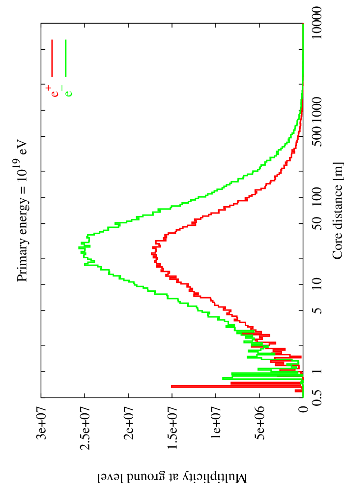
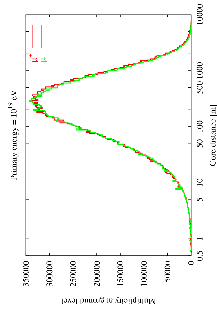

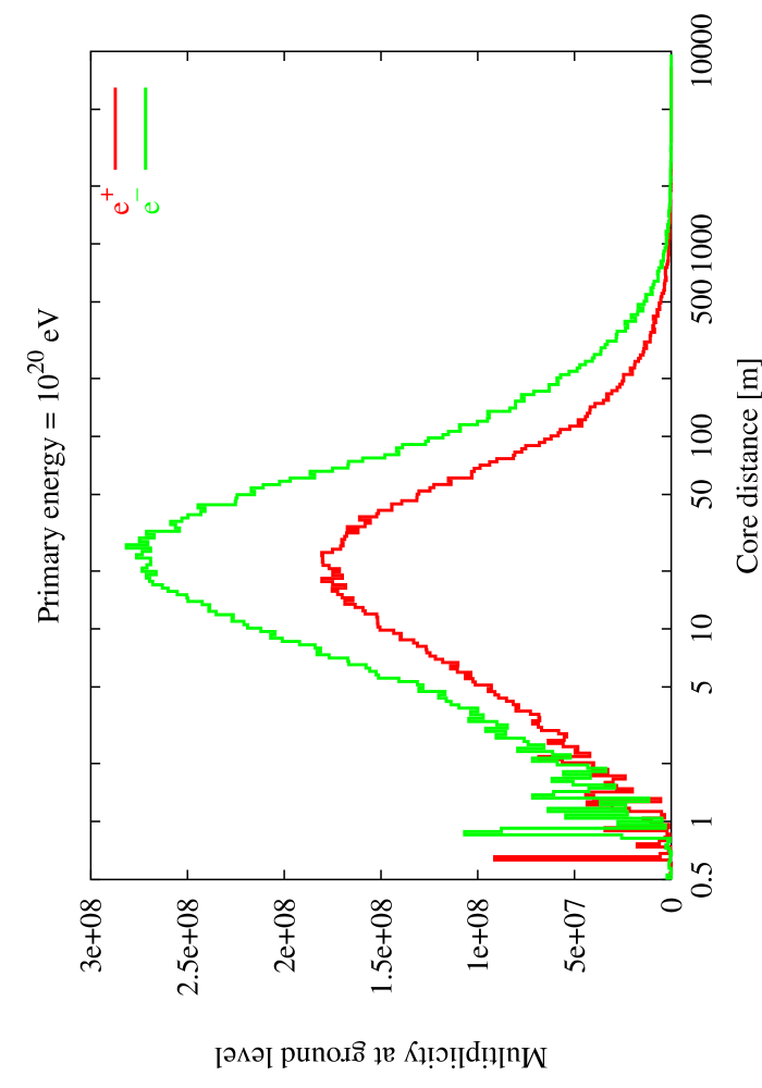
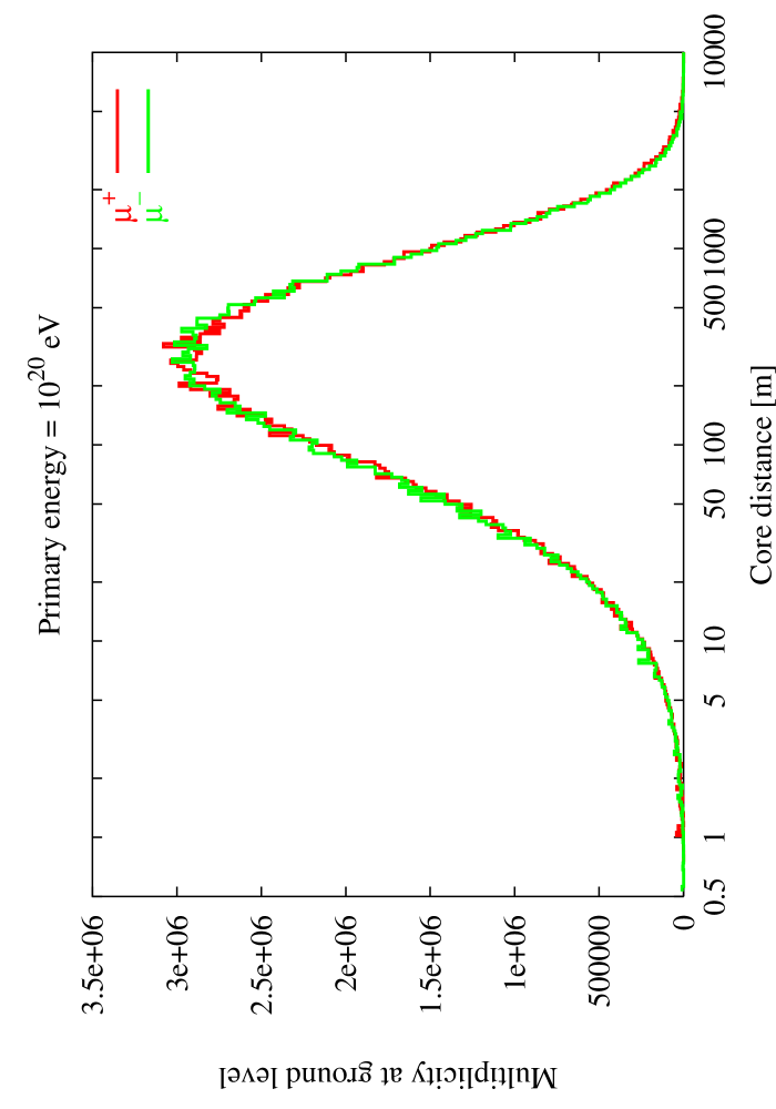


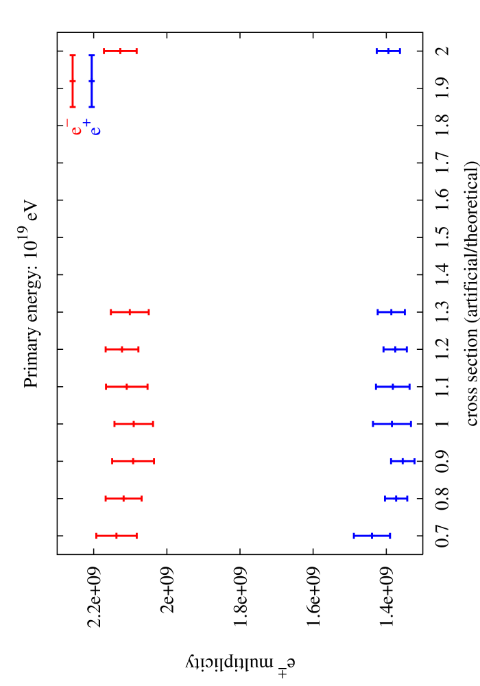
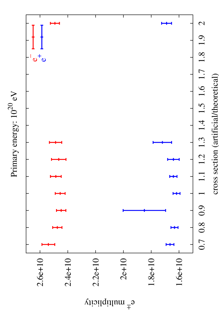
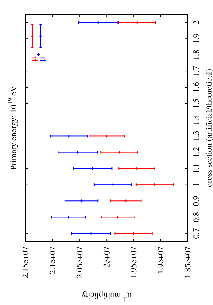
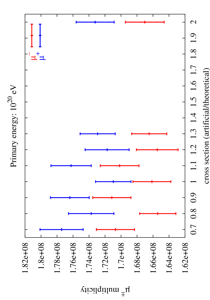
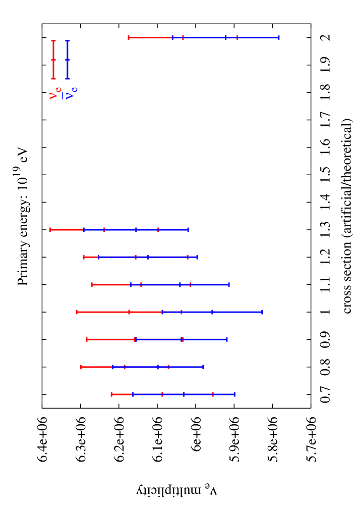
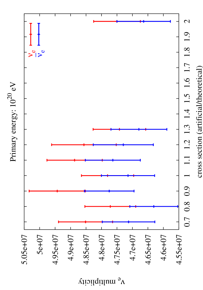
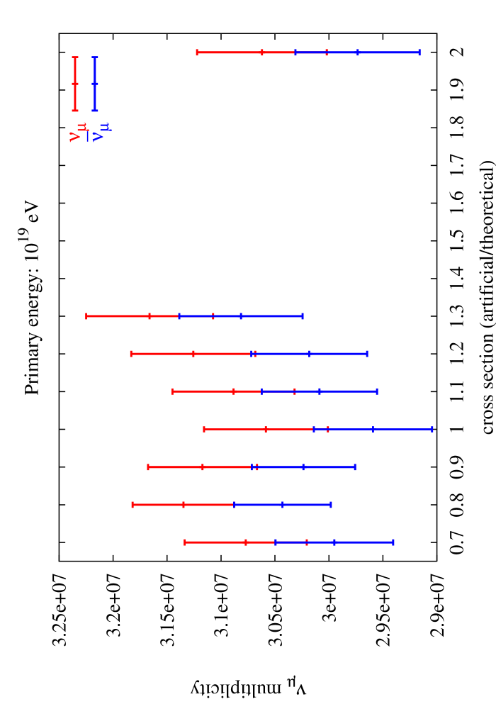
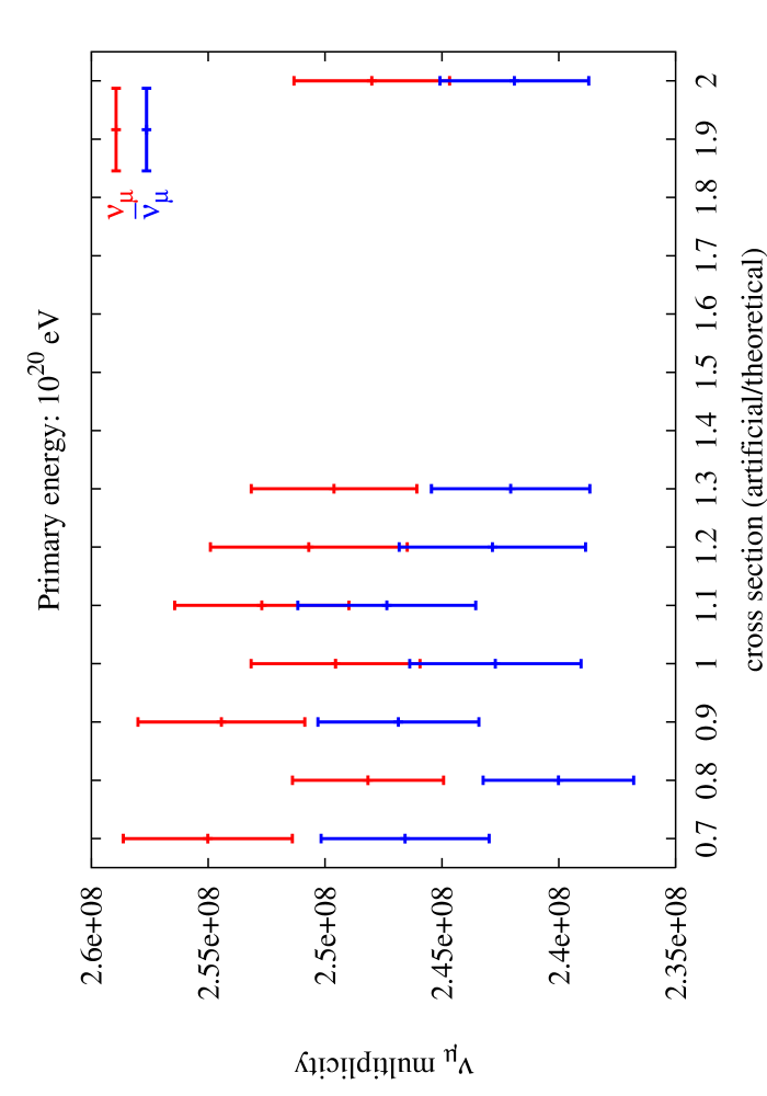


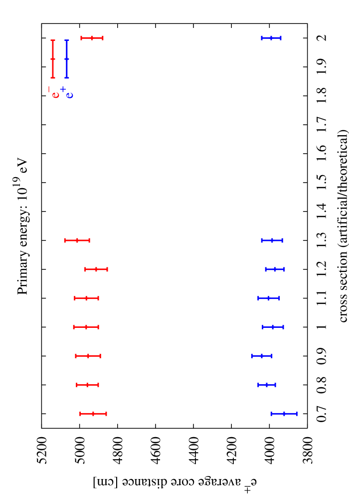
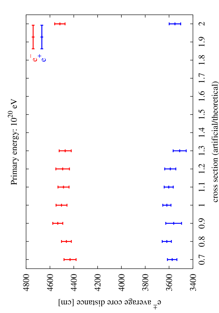
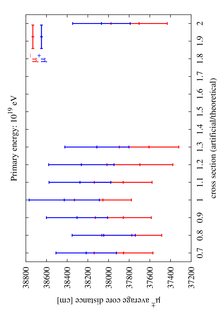
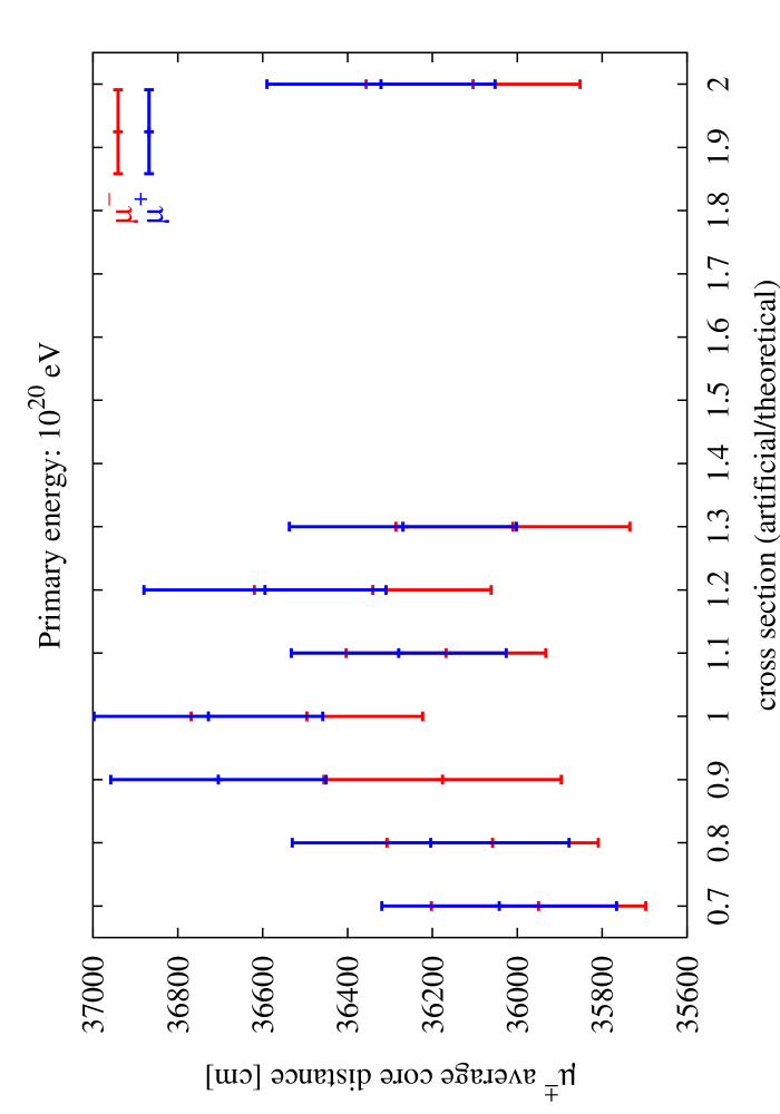
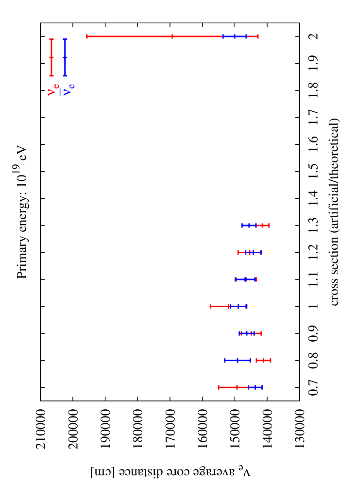
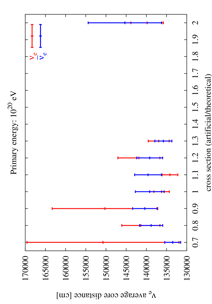
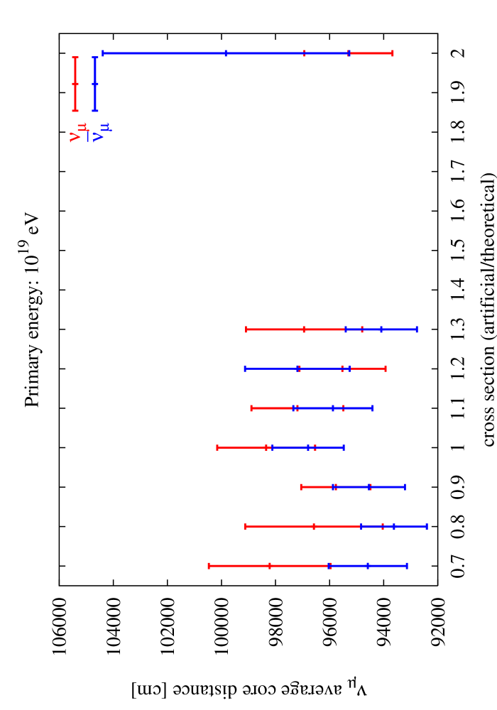
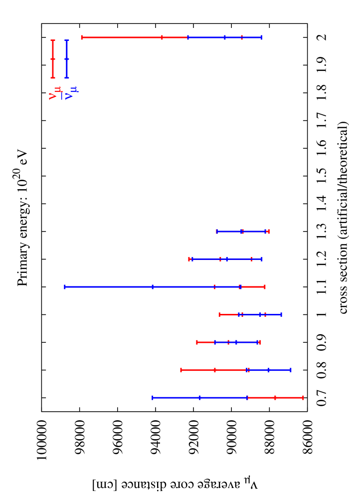
Chapter 7 Searching for extra dimensions in high energy cosmic rays:
the fragmentation of mini black holes
7.1 Background on the topic
Extra Dimensions have been around the theory landscape for some time, starting from the 20’s with the work of Kaluza and Klein. Their original idea was to use a five dimensional manifold, the fifth dimension being a circle, and identify the component of the metric in this 5-dimensional space as a 4-dimensional vector field. The field, after a Fourier expansion in the extra variable, has a massless component which can be identified with the photon, plus an infinite tower of massive states. The masses of these additional states are inversely proportional to the size of the extra dimensions and their disappearance from the low energy spectrum can be simply obtained by tuning the extra dimensions appropriately. Then, the natural question to ask is: how large can the extra dimensions be without getting into conflict with the experiment? The answer to this question requires the Standard Model fields to be localized on the brane with gravity free to propagate in the extra space, called “the bulk”. This scenario is characterized by a rich phenomenology, as we are going to discuss next, with implications which may appear also in the structure of cosmic ray showers. One possibility is the formation, due to a lower gravity scale, of mini black holes which decay into an “s-wave” or isotropically into all the particles of the Standard Model. For this reason we present a study of the main observables of the air showers initiated by an incoming primary which collides with the atmosphere and characterized by the formation of an intermediate mini black hole. We study particle multiplicities, lateral distributions and the ratio of the electromagnetic to the hadronic components of these special air showers. In this chapter we illustrate a simulation study of the resulting cascades over the entire range (eV) of ultra high initial energies, for several values of the number of large extra dimensions, for a variety of altitudes of the initial interaction and with the energy losses in the bulk taken into account. The results are compared with a representative of the standard events, namely the shower due to the collision of a primary proton with a nucleon in the atmosphere. Both the multiplicities and the lateral distribution of the showers show important differences between the two cases and, consequently, may be useful for the observational characterization of the events. The electromagnetic/hadronic ratio is strongly fluctuating and, thus, less decisive for the altitudes considered.
This chapter is based on the paper [32].
7.2 Introduction
In the almost structureless fast falling with energy inclusive cosmic ray spectrum, two kinematic regions have drawn considerable attention for a long time [8, 112]. These regions are the only ones in which the spectral index of the cosmic ray flux shows a sharper variation as a function of energy, probably signaling some “new physics”, according to many. These two regions, termed the knee and the ankle [77] have been puzzling theorists and experimentalists alike and no clear and widely accepted explanation of this unusual behaviour in the propagation of the primaries - prior to their impact with the earth atmosphere - exists yet. A large experimental effort [11, 57] in the next several years will hopefully clarify several of the issues related to this behaviour.
While the ankle is mentioned in the debate regarding the possible existence of the so called Greisen, Zatsepin and Kuzmin (GZK) cutoff [76], due to the interaction of the primaries with the cosmic background radiation, the proposed resolutions of this puzzle are several, ranging from a resonant Z-burst mechanism [120] to string relics and other exotic particle decays [17, 16, 18, 43]. The existence of data beyond the cutoff has also been critically discussed [13].
Given the large energy involved in the first stage of the formation of the air showers, the study of the properties of the cascade should be sensitive to any new physics between the electroweak scale and the original collision scale. Especially in the highest energy region of the spectrum, the energy available in the interaction of the primaries with the atmospheric nuclei is far above any conceivable energy scale attainable at future ground-based accelerators. Therefore, the possibility of detecting supersymmetry, for instance, in cosmic ray showers has also been contemplated [42]. Thus, it is not surprising, that most of the attempts to explain these features of the cosmic ray spectrum typically assume some form of new physics at those energies.
With the advent of theories with a low fundamental scale of gravity [10] and large compact or non-compact extra dimensions, the possibility of copiously producing mini black holes (based on Thorne’s hoop conjecture [111]) in collisions involving hadronic factorization scales above 1 TeV has received considerable attention [48] [68] and these ideas, naturally, have found their way also in the literature of high energy cosmic rays [7, 60] and astrophysics [37]. For instance, it was recently suggested that the long known Centauro events might be understood as evaporating mini black holes, produced by the collision of a very energetic primary (maybe a neutrino) with a nucleon (quark) in the atmosphere [99]. Other proposals [69] also either involve new forms of matter (for example strangelets) or speculate about major changes in the strong interaction dynamics [124].
While estimates for the frequencies of these types of processes both in cosmic rays [1, 7, 99] and at colliders [68] have been presented, detailed studies of the multiplicities of the particles collected at the detectors, generated by the extensive atmospheric air showers following the first impact of the primary rays, are far from covering all the main features of the cascade [125]. These studies will be useful in order to eventually disentangle new physics starting from an analysis of the geometry of the shower, of the multiplicity distributions of its main sub-components [27] and of its directionality from deep space. For instance, the study of the location of the maxima of the showers at positions which can be detected by fluorescence mirrors [5], generated as they go across the atmosphere, and their variations as a function of the parameters of the underlying physical theory, may help in this effort [1]; other observables which also contain potential new information are the multiplicities of the various particle sub-components and the opening of the showers as they are detected on the ground [27]. We will focus on this last type of observables.
To summarize: in the context of the TeV scale gravity with large extra dimensions it is reasonable to assume that mini black holes, black holes with mass of a few TeV, can form at the first impact of ultra high energy primary cosmic rays with nucleons in the atmosphere. The black hole will evaporate into all types of particles of the Standard Model and gravity. The initial partons will hadronize and all resulting particles as they propagate in the atmosphere will develop into a shower(s), which eventually will reach the detectors. The nature and basic characteristics of these showers is the question that is the main subject of the present work. What is the signature on the detector of the showers arising from the decay of such mini black holes and how it compares with a normal (not black hole mediated) cosmic ray event, due, for instance, to a primary proton with the same energy colliding with an atmospheric nucleon (the "benchmark" event used here). The comparison will be based on appropriate observables of the type mentioned above.
Our incomplete control of the quantum gravity/string theory effects, of the physics of low energy non-perturbative QCD and of the nature of the quark-gluon plasma phase in QCD, makes a fully general analysis of the above phenomena impossible at this stage. To proceed, we made the following simplifying assumptions and approximations. (1) The brane tension was assumed much smaller than the fundamental gravity scale, so it does not modify the flat background metric. It is not clear at this point how severe this assumption is, since it is related to the “cosmological constant problem” and to the concrete realization of the Brane-World scenario. (2) The black hole was assumed to evaporate instantly, leading to initial “partons”, whose number and distributions are obtained semiclassically. No virtual holes were discussed and no back reaction was taken into account. (3) The initial decay products were assumed to fly away and hadronize, with no intermediate formation of a quark-gluon plasma or of a disoriented chiral condensate (DCC). (4) We used standard simulation programs for the investigation of the extensive air showers produced in the cases of interest. To this purpose, we have decided to use the Monte Carlo program CORSIKA [78] with the hadronic interaction implemented in SIBYLL [62] in order to perform this comparison, selecting a benchmark process which can be realistically simulated by this Monte Carlo, though other hadronization models are also available [83]. Finally, (5) a comment is in order about our selection of benchmark process and choice of interesting events. In contrast to the case of a hadronic primary, the mini black hole production cross section due to the collision of a TeV neutrino with a parton is of the order of the weak interaction neutrino-parton cross section [99]. It would, thus, be interesting to compare the atmospheric showers of a normal neutrino-induced cosmic ray event to one with a black hole intermediate state. Unfortunately, at present neutrinos are not available as primaries in CORSIKA, a fact which sets a limitation on our benchmark study. However, it has to be mentioned that neutrino scattering off protons is not treated coherently at very high energy, since effects of parton saturation have not yet been implemented in the existing codes [27]. As shown in [88] these effects tend to lower the cross section in the neutrino case. For a proton-proton impact, the distribution of momenta among the partons and the presence of a lower factorization scale should render this effect less pronounced. For these reasons we have selected as benchmark process a proton-to-air collision at the same depth () and with the same energy as the corresponding “signal event”. In order to reduce the large statistical fluctuations in the formation of the extensive air showers after the collisions, we have chosen at a first stage, in the bulk of our work, to simulate collisions taking place in the lower part of the atmosphere, up to 1 km above the detector, in order to see whether any deviation from a standard scattering scenario can be identified. Another motivation for the analysis of such deeply penetrating events is their relevance in the study of the possibility to interpret the Centauro events as evaporating mini black holes [99]. A second group of simulations have been performed at a higher altitude, for comparison.
The present chapter consists of seven sections, of which this Introduction is the first. In Section 7.3 we briefly describe the D-brane world scenario, in order to make clear the fundamental theoretical assumptions in our study. A brief review of the properties of black holes and black hole evaporation is offered here, together with all basic semiclassical formulas used in the analysis, with the dependence on the large extra dimensions shown explicitly. In Section 7.4 a detailed phenomenological description of the modeling of the decay of the black hole is presented, which is complementary to the previous literature and provides an independent characterization of the structure of the decay. Incidentally, a Monte Carlo code for black hole decay has also been presented recently [89]. We recall that this description -as done in all the previous works on the subject- is limited to the Schwarzschild phase of the lifetime of the mini black hole. The modeling of the radiation emission from the black hole - as obtained in the semiclassical picture - (see [84] for an overview) is performed here independently, using semi-analytical methods, and has been included in the computer code that we have written and used, and which is interfaced with CORSIKA. Recent computations of the greybody factors for bulk/brane emissions [84], which match well with the analytical approach of [85] valid in the low energy limit of particle emission by the black hole, have also been taken into account. Section 7.5 contains our modeling of the hadronization process. The hadronization of the partons emitted by the black hole is treated analytically in the black hole rest frame, by solving the evolution equations for the parton fragmentation functions, making use of a special algorithm [25] and of a specific set of initial conditions for these functions [87]. After a brief discussion in Section 7.6 of the transformation of the kinematics of the black hole decay event from the black hole frame to the laboratory frame, we proceed in Section 7.7 with a Monte Carlo simulation of the extensive air showers of the particles produced by taking these particles as primaries. The simulations are quite intensive and have been performed on a small computer cluster. As we have already mentioned, in this work we focus on the multiplicities, on the lateral distributions of the events and on the ratio of electromagnetic to hadronic energies and multiplicities and scan the entire ultra high energy part of the cosmic ray spectrum. Our results are summarized in a series of plots and are commented upon in the final discussion in Section 7.8.
7.3 TeV Scale Gravity, Large Extra Dimensions and Mini Black Holes
The theoretical framework of the present study is the D-brane world scenario [10]. The World, in this scenario, is 10 dimensional, but all the Standard Model matter and forces are confined on a dimensional hypersurface (the -brane). Only gravity with a characteristic scale can propagate in the bulk. The longitudinal dimensions are constrained experimentally to be smaller than . However, for our purposes these dimensions may be neglected, since the Kaluza-Klein excitations related to these have masses at least of , too large to affect our discussion below. Consistency with the observed Newton’s law, on the other hand, leads to the relation , between GeV, the fundamental gravity scale and the volume of the dimensional compact or non-compact transverse space. A natural choice for , dictated a priori by the “gauge hierarchy” puzzle, is (1 TeV), while the simplest choice for the transverse space is an -dimensional torus with all radii equal to . Thus, one obtains a condition between the number and the size of the transverse dimensions. Notice that under the above assumptions and for all values of , is much larger than cm, the length scale at which one traditionally expects possible deviations from the 3-dimensional gravity force, and the corresponding dimensions are termed “large extra dimensions” (LED). For one obtains of the order of a fraction of a mm. At distances much smaller than one should observe -dimensional Newton’s law, for instance, as in torsion balance experiments [91]. Current bounds on the size of these large extra dimensions and on come from various arguments, mostly of astrophysical (for instance TeV for ) or cosmological ( TeV for ) origin [84]. A larger number of LED () translates into a reduced lower bound on . It should be pointed out, that in general it is possible, even if “unnatural”, that the transverse space has a few dimensions large and the others small. Here we shall assume a value of of order 1TeV, neglect the small extra dimensions and treat the number of LED () as a free parameter.
The implications of the existence of LED are quite direct in the case of black hole physics. The black hole is effectively 4-dimensional if its horizon () is larger than the size of the extra dimensions. In the opposite case (, or equivalently for black hole masses kg for [99]) it is dimensional, it spreads over the full space and its properties are those of a genuine higher dimensional hole. According to some estimates, over which however there is no universal consensus [119], black holes should be produced copiously [48] [67] in particle collisions, whenever the center of mass energy available in the collision is considerably larger than the effective scale (). With 1 TeV, one may contemplate the possibility of producing black holes with masses of order a few TeV.
Their characteristic temperature is inversely proportional to the radius of the horizon, or roughly of order and evaporate by emitting particles, whose mass is smaller than . The radiation emitted depends both on the spin of the emitted particle, on the dimension of the ambient space and on the amount of back-scattering outside the horizon, contributions which are commonly included in the so called “greybody factor”, which are particularly relevant in the characterization of the spectrum at lower and at intermediate energy. A main feature of the decaying mini black hole is its large partonic multiplicity, with a structure of the event which is approximately spheroidal in the black hole rest frame.
Once produced, these mini black holes evaporate almost instantly. The phenomenological study of 4-dimensional black holes of large mass and, in particular, of their Hawking radiation [90] [103] [93], as well as the study of the scattering of states of various spins () on a black hole background, all performed in the semiclassical approximation, have a long history. For rotating black holes one identifies four phases characterizing its decay, which are (1) the balding phase (during which the hole gets rid of its hair); (2) the spin-down phase (during which the hole slows down its rotational motion); (3) the Schwarzschild phase (the usual semiclassically approximated evaporation phase) and, finally, (4) the Planck phase (the final explosive part of the evaporation process, with important quantum gravitational contributions). Undoubtedly, the best understood among these phases is the Schwarzschild phase, which is characterized by the emission of a (black body) energy spectrum which is approximately thermal, with a superimposed energy-dependent modulation, especially at larger values of the energy. The modulation is a function of the spin and is calculable analytically only at small energies. Extensions of these results to 4+n dimensions are now available, especially in the Schwarzschild phase, where no rotation and no charge parameter characterize the background black hole solutions. Partial results exist for the spin down phase, where the behaviour of the greybody factors have been studied (at least for 1 additional extra dimension) both analytically and numerically. The Planck phase, not so relevant for a hole of large mass (say of the mass of the sun ( gr) which emits in the nano-Kelvin region, is instead very relevant for the case of mini-black holes, for which the separation between the mass of the hole and the corresponding (effective) Planck mass gets drastically reduced as the temperature of the hole raises and the back-reaction of the metric has to be taken into account.
In the discussion below we shall use the semiclassical formulas derived for large black holes in the Schwarzschild phase and naively extrapolate them to the mini black holes as well. This is not, we believe, a severe approximation for the phenomena we shall discuss. As the hole evaporates, it looses energy, its mass decreases, its temperature increases and the rate of evaporation becomes faster. Thus, the lifetime of the hole is actually shorter than the one derived ignoring the back reaction. As we shall see below, the naive lifetime is already many orders of magnitude smaller than the hadronization time. This justifies the use of the “sudden approximation” we are making of the decay process and explains why the neglect of the back reaction is not severe.
We recall that the metric of the dimensional hole in the Schwarzschild phase is given by [101]
| (7.1) |
where denotes the number of extra spacelike dimensions, and is the area of the ()-dimensional unit sphere which, using coordinates and , with takes the form
| (7.2) |
The temperature of the black hole is related to the size of its horizon by [101]
| (7.3) |
and the formula for the horizon can be expressed in general in terms of the mass of the black hole and the gravity scale [101]
| (7.4) |
For and GeV it reproduces the usual formula for the horizon () of a 4 dimensional black hole. For the relation between and becomes nonlinear and the presence of in the denominator of Eq. (7.4) in place of increases the horizon size for a given . For and TeV the size of the horizon is around fm and decreases with increasing .
In the Schwarzschild/spin-down phase, the number of particles emitted per unit time by the black hole as a function of energy is expressed in terms of the absorption/emission cross sections (or equivalently of the greybody factors ), which, apart from , depend on the spin of the emitted particle, the angular momentum of the partial wave and the corresponding energy ,
| (7.5) |
Multiplying the rate of emitted particles per energy interval by the particle energy one obtains for the power emission density
| (7.6) |
where the sum is over all Standard Model particles and the +() in the denominator correspond to fermions (bosons), respectively. are the cross sections for the various partial waves and depend on the spin of each particle. We recall, that in the geometric optics approximation a black hole acts as a perfect absorber of slightly larger radius than [110], which can be identified as the critical radius for null geodesics
| (7.7) |
The optical cross section is then defined in function of (or equivalently via Eq. (7.7)), such that , the effective surface area of the black hole hole projected over a k-dimensional sub-manifold becomes [56]:
| (7.8) |
and
| (7.9) |
is the volume of a k-sphere.
It is convenient to rewrite the greybody factors as a dimensionless constant normalized to the effective area of the horizon , obtained from (7.8) setting and
| (7.10) |
and replacing the particle cross section in terms of a thermal averaged graybody factor (, denoting the spin or species [102]). Eqs. (7.5) integrated over the frequency give (for particle )
| (7.11) |
with
| (7.12) |
where is the number of degrees of freedom of particle and is defined by the integral ( is the spin)
| (7.13) |
from which for bosons (fermions). These numbers depend on the dimension of the brane, which in our case is 3. and are the Gamma and the Riemann function respectively. Since depends on the temperature (via ), after some manipulations one obtains
| (7.14) |
and
| (7.15) |
Summing over all the particles we obtain the compact expression
| (7.16) |
with
| (7.17) |
The emission rates are given by
| (7.18) |
| (7.19) |
| (7.20) |
for particles with respectively. Furthermore, integration of Eq. (7.6) gives for the black hole mass evolution
| (7.21) | |||||
with
| (7.22) |
where now for bosons (fermions). Taking the ratio of the two equations (7.21) and (7.16) we obtain
| (7.23) | |||||
where we have defined
| (7.24) |
and
| (7.25) |
This formula does not include corrections from emission in the bulk.
In the “sudden approximation” in which the black hole decays at its original formation temperature one easily finds , where is the energy spectrum of the decay products, and using Boltzmann statistics one obtains the expression [48]
| (7.26) |
This formula is approximate as are all the formulas for the multiplicities. A more accurate expression is obtained integrating Eq. (7.23) to obtain
| (7.27) |
and noticing that the entropy of a black hole is given semiclassically by the expression
one finds that
which can be computed numerically for a varying . As one can see from Fig. 7.1, the two formulas for the multiplicities are quite close, as expected, but Eq. (7.26) gives larger values for the multiplicities compared to (7.3) as noted by [33]. Other expressions for the multiplicities can be found in [34].
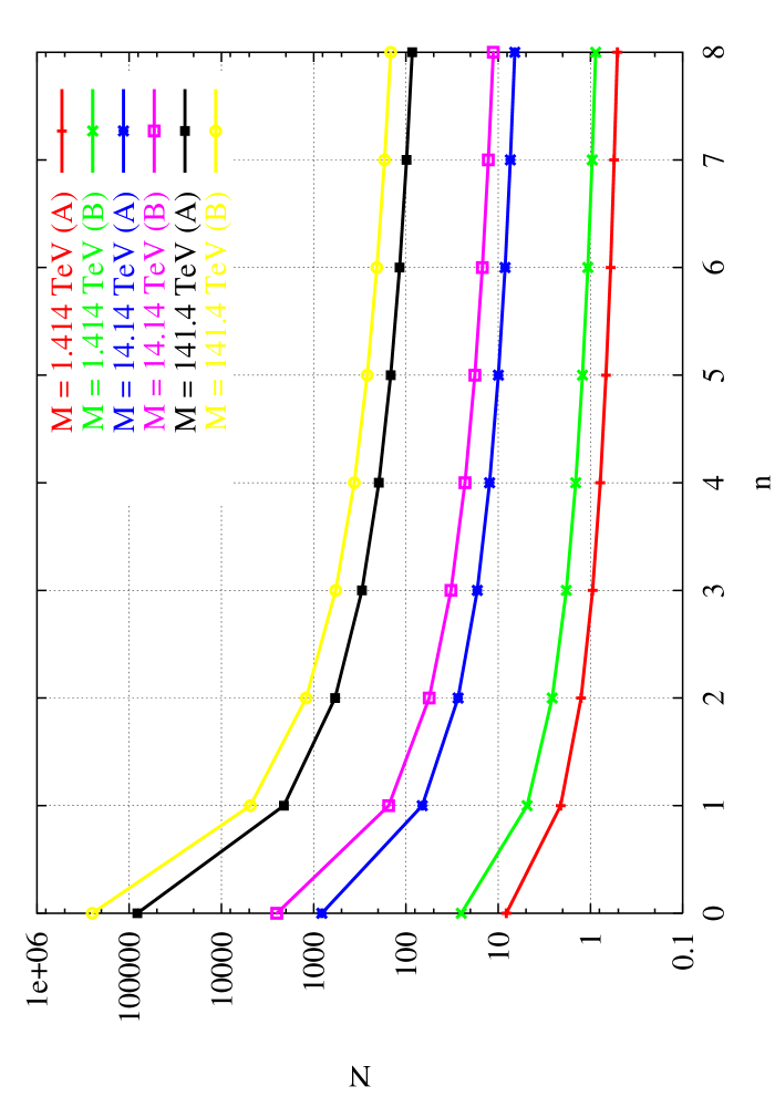
Since the number of elementary states becomes quite large as we raise the black hole mass compared to the (fixed) gravity scale, and given the (large) statistical fluctuations induced by the formation of the air shower, which reduce the dependence on the multiplicity formula used, we will adopt Eq. (7.26) in our simulations. Overall, in the massless approximation, the emission of the various species for a 3-brane is characterized by approximately into spin zero, into spin half and into spin one particles, with similar contributions also for the power emissivities. These numbers change as we vary the dimension of the brane (d) and so does the formula for the emissivities, since the number of brane degrees of freedom has to be recomputed, together with the integrals on the emission spectra [1].
The integration of the equation for the power spectrum, in the massless approximation, can be used to compute the total time of decay (assuming no mass evolution during the decay)
| (7.28) |
which implies that at an energy of approximately 1 TeV the decay time is of the order of seconds. Therefore strong interaction effects and gravity effects appear to be widely separated and hadronization of the partons takes place after their crossing of the horizon. The black hole is assumed to decay isotropically (s-wave) to a set of elementary states, selected with equal probability from all the possible states available in the Standard Model. We mention that in most of the analysis presented so far [60, 7, 1] the (semiclassical) energy loss due to bulk emission has not been thoroughly analyzed. We will therefore correct our numerical studies by keeping into account some estimates of the bulk emission.
7.4 Modeling of the Black Hole Decay
The amount of radiation emitted by the black hole in the ED is viewed, by an observer living on the brane, as missing energy compared to the energy available at the time when the black hole forms. From the point of view of cosmic ray physics missing energy channels imply reduced multiplicities in the final air shower and modified lateral distributions, these two features being among the main observables of the cosmic ray event. However, since the initial energy of the original cosmic ray is reconstructed by a measurement of the multiplicities, an event of reduced multiplicity will simply be recorded as an event of lower energy. It is then obvious that an additional and independent reconstruction of the energy of the primary cosmic ray is needed in order to correctly identify the energy of these events.
In our study we will compute all the observables of the induced air shower using both the lab frame (LF) and the black hole frame (BHF) to describe the impact and the formation of the intermediate black hole resonance. Also, in the simulations that we will perform, the observation level at which we measure the properties of the air showers will be selected to take properly into account the actual position of a hypothetical experimental detector. The target of the first impact of mass is assumed to be a nucleon (or a quark) at rest in the atmosphere and the center of mass energy, corrected by emission loss in the bulk, is made promptly available for an instantaneous black hole formation and decay. We will also assume that the energy of the incoming primary varies over all the highest part of the cosmic ray spectrum, from eV up to eV.
We denote by the speed of the black hole in the lab frame. In our notations, is the typical energy of each elementary state in the decay products (parton, lepton) in the BH frame and is its corresponding momentum.
We will assume that a black hole decays “democratically” into all the possible partonic states, proportionally to the number of Standard Model states which are available to it at a given energy.
The energy per partonic channel will be appropriately weighted and we will assume that each parton will decay into a final state hadron (carrying a fraction of the original momentum), with a probability distribution given by the corresponding fragmentation function , which is evolved from some low energy input scale up to the relevant scale characterizing the decay. This is given by the available energy per fundamental state, equally distributed among all the states.
The quantification of the injection spectrum involves a computation of the relevant probabilities for the formation of all the possible hadronic/leptonic states prior to the simulation of the air shower. Let’s briefly elaborate on this.
To move from the parton level to hadron level, we let , , and be the fragmentation functions of quarks , antiquarks , and of the gluon , respectively, into some hadron with momentum fraction at the scale . From the fragmentation functions we obtain, for each hadron , the mean multiplicity of the corresponding s-wave and the corresponding average energy and momentum. Specifically we obtain
| (7.29) |
for the probability of producing a hadron , and
| (7.30) |
for the average energy of the same hadron. We recall that is the minimal fraction of energy a hadron , of mass , can take at a scale , and can be defined as . In practical applications one can take the nominal value for every hadron, without affecting much the mean multiplicities and the related probabilities. This implies that
together with the condition , where the sum runs over all the types of hadrons allowed by the fragmentation. In all the equations above, the fragmentation takes place at the typical scale , scale at which the moments are computed numerically. For the identification of the probabilities it is convenient to organize the 123 fundamental states of the Standard Model into a set of flavour states , with running over all the flavours except for the top quark, where in we lump antiquark states and color states, plus some additional states. The weight of the set is , where the factors 2 and 3 refer to spin, quark-antiquark degeneracy and color. It is worth to recall that quark and antiquark states of the same flavour have equal fragmentation functions in all the hadrons, and this justifies the degeneracy of the set. The additional states are the gluon (g) with a weight , the photon , with a weight and the remaining states in which we lump all the states which have been unaccounted for, whose probabilities are computed by difference. These include the top and the antitop , the W’s and Z and the leptons . The fragmentation functions into hadrons, corresponding to these states, are computed by difference from the remaining ones , and , which are known at any scale from the literature. Beside the favour index , introduced above, we introduce a second index running over the states, the photon and the gluons .
The probability of generating a specific sequence of states in the course of the evaporation of the black hole is then given by a multinomial distribution of the form
| (7.31) |
which describes a typical multi-poissonian process with trials. Notice that, to ensure proper normalization, we need to require that
| (7.32) | |||||
The computation of the cumulative probabilities to produce any number of hadrons of type by the decay of the black hole are obtained from the multinomial distribution multiplied by the fragmentation probabilities of each elementary state into and summing over all the possible sequences
| (7.33) |
A possible way to compute when is large is to multiply the multinomial distribution by a suppression factor , with a very large number, and interpret this factor as a Boltzmann weight, as in standard Monte Carlo computations of the partition function for a statistical system. Simulations can be easily done by a Metropolis algorithm and the configurations of integers selected are those for which the normalization condition is satisfied. In our case, since we are interested only in the mean number of hadrons produced in the decay and in their thermal spectrum, the computation simplifies if we average over all the relevant configurations.
7.5 Fragmentation and the Photon Component
The evolution with of the fragmentation functions is conveniently formulated in terms of the linear combinations
| (7.34) | |||||
| (7.35) | |||||
| (7.36) |
as for these the gluon decouples from the non–singlet and the asymmetric combinations, leaving only the singlet and the gluon fragmentation functions coupled;
| (7.37) | |||||
| (7.38) | |||||
| (7.39) | |||||
| (7.40) | |||||
The kernels that appear in the equations above are defined by
| (7.41) | |||||
| (7.42) | |||||
| (7.43) |
with being the QCD coupling constant. In the perturbative expansion of the splitting functions,
| (7.44) |
The timelike kernels that we use are given by
| (7.45) | |||||
| (7.46) | |||||
| (7.47) | |||||
| (7.48) | |||||
| (7.49) | |||||
The formal solution of the equations is given by
| (7.50) |
where is the starting scale of the initial conditions, given by . At leading order in , we solve this equation using a special ansatz
| (7.51) |
and generating recurrence relations at the order for the coefficients in terms of the [25]. It is easy to see that this corresponds to the numerical implementation of the formal solution
| (7.52) |
with , where the exponential is a formal expression for an infinite iteration of convolution products. We show in Figures 7.2-7.4 results for some of the fragmentation functions into pions, kaons and protons computed for a typical parton scale of 200 GeV.


The photon contributions to the decay of the black hole is treated separately. The evolution equation for the fragmentation functions of photons and parton fragmentation into photon satisfy at leading order in (the QED fine structure constant) and (the QCD coupling), the evolution equations [86]
| (7.53) |
which can be integrated with the initial conditions , and
| (7.54) |
which can also be integrated with the result [65]
| (7.55) |
In Eq. (7.55) the second term is termed the hadronic boundary conditions, which come from an experimental fit, while the first term is the pointlike contributions, which can be obtained perturbatively. In [3] a leading order fit was given
| (7.56) |
at the starting scale GeV. The kernels in these cases are given by simple modifications of the ordinary QCD kernels, for instance [86].
For the fragmentation function of quarks to photons with virtuality , the perturbative result is given in [105]
| (7.57) |
where is the virtuality of the photon. The gluon to photon transitions are neglected, since vanishes in leading order.
We recall that each elementary state emitted is characterized by an average energy given by .
The leptonic component , , produced by the decay is left unaltered and provides an input for the air shower simulator as soon as these particles cross the horizon. The s are left to decay into their main channels, while the hadronization of the quarks and the gluons is treated with our code, that evolves the fragmentation functions to the energy scale . The top () quark is treated consistently with all its fundamental decays included; hadronization of the quark is treated with suitable fragmentation functions and also involves a suitable evolution. As we vary and we scan over the spectrum of the incoming cosmic rays the procedure is repeated and rendered automatic by combining in a single algorithm all the intermediate steps. Tables 1 and 2 contain the results of a renormalization group analysis of the fragmentation functions for all the partons (except the top quark), where we show both the initial conditions at the input scale, whose lowest value is GeV, and the results of the evolution, at a final scale of GeV, the initial set being taken from ref. [87].
| u | ||||||
|---|---|---|---|---|---|---|
| d | ||||||
| s | ||||||
| c | ||||||
| b | ||||||
| g | ||||||
| u | ||||||
|---|---|---|---|---|---|---|
| d | ||||||
| s | ||||||
| c | ||||||
| b | ||||||
| g | ||||||
This concludes the computation of the probabilities for each hadron/lepton present in the decay products of the mini black hole. It is reasonable to assume that these particles will be produced spherically, since higher angular momenta are suppressed by the corresponding centrifugal barrier. However, the analysis of the shower profile has to be performed in the lab frame. This requires the transformation of the initial configurations above to the laboratory frame, which is exactly what is discussed next.
7.6 Sphericity and Boost
The transformation from the black hole frame (BHF) to the laboratory frame (LF) is performed by a Lorentz boost with speed , the speed of the black hole in the LF. Assuming that the black hole is produced in the collision of a primary of energy in the LF and negligible mass compared to , with a parton of mass in the atmosphere, one obtains . A spherical distribution of a particular particle of mass among the decay products in the BHF is transformed to an elliptical one, whose detailed form is conveniently parametrized by
| (7.58) |
where is the speed of this particle in the BHF, the ratio of its BHF momentum and energy. Figure 7.5 depicts the relevant kinematics. A particle emitted in the direction in the BHF, is seen in the direction in the LF, with
| (7.59) |
For values of the shape of the 1-particle distribution in the LF is characterized by a maximum angle of emission
| (7.60) |
which for is equal to . Only for there is backward emission in the LF.


As a relevant example, let us consider the case of a hadron of mass GeV and energy GeV emitted by a black hole, formed by an initial primary of energy TeV, which hit a quark of mass MeV to form a black hole. The gives and the corresponding maximum angle in the LF is , giving an angular opening of the decay products of about 2 degrees.
As shown in Figure 7.5, for , which is relevant for our purposes, the mapping from to is not one to one. In a given direction in the LF, one receives particles emitted in two different directions in the BHF. They satisfy [24]
| (7.61) |
where
| (7.62) |
and with the momenta and energies of the two branches given by
| (7.63) |
and
| (7.64) |
respectively. In the above formulas , is the speed of the hadron in the LF (BHF), and . For massless final state particles, in particular, these relations become
| (7.65) |
and reduce to the familiar Doppler formula when .
The probability distribution of a hadron (h) as a function of the direction in the BHF, assumed spherically symmetric and normalized to the total probability of detecting this hadron among the decay products with elementary states, is
| (7.66) |
The corresponding one in the LF is
| (7.67) |
In the special case , the probability distribution simplifies to
| (7.68) |
peaked in the forward direction, symmetric around the maximum value, obtained for and equal to , while the momentum distribution is
| (7.69) |
As we have already mentioned, the structure of the partonic event (and, similarly, of the hadronic event after fragmentation) is characterized by the formation of an elliptical distribution of partons, strongly boosted toward the detector along the vertical direction. Each uniform (s-wave) distribution is strongly elongated along the arrival direction (due to the large speed of the black hole along this direction) and is characterized by two sub-components (), identified by a superscript. Their sum is the total probability distribution given in (7.61). The “+” momentum component is largely dominant and strongly peaked around the vertical direction with rather small opening angles and this behaviour can be analyzed numerically with its dependence. In the explicit identification of the two independent distributions in terms of the opening angle , as measured in the LF, we use the relations
| (7.70) |
where we have introduced a factor of 1/2 for a correct normalization of the new distribution in the variable. In Figures 7.7 and 7.7 we show the structure of these distributions in the LF. Both are characterized by a very small opening angle () with respect to the azimuthal direction of the incoming cosmic ray, being the dominant one. Two similar plots (Figures 7.9 and 7.9) illustrate the two components as functions of the same angle.


One can easily check that we can now integrate symmetrically on both distributions to obtain the correct normalization (to ) for a given hadron (or parton)
| (7.71) |
or, equivalently, using as a distribution variable
| (7.72) |
with
| (7.73) |
and obtained from (7.60).
7.7 Air Shower Simulations
The simulation of the events is performed at the last stage, using an air shower simulator. We have used CORSIKA [78] with appropriate initial conditions on the spectrum of the incoming particles in order to generate the full event measured at detector level. In most of the simulations we have assumed that the first impact takes place in the lower part of the atmosphere, not far from the level of the detector, at a varying altitude. The reason is that one of our interests is the investigation of the possibility that the Centauro events may be related to evaporating mini black holes, formed by the collision of weakly interacting particles (e.g. neutrinos) which penetrate the atmosphere. Of course, we have simulated events happening at higher altitudes as well. We have performed two separate sets of simulations, the first set being benchmark events with an “equivalent” proton replacing the neutrino-nucleon event, colliding at the same height, the second being the signal event, i.e. the black hole resonance. The difference between the first and the second set is attributed to the different components of the final state prior to the development of the air shower.
We compute the average number of particles produced in the process of BH evaporation using the formula
| (7.74) |
where is the energy in the center of mass frame in the neutrino-nucleon collision and is the fraction of that is bound into the black hole as a function of the number of extra-dimensions. Numerical values for in head-on collisions are taken from Ref. [50] and reported in Table 7.3.
| 0 | |
|---|---|
| 1 | |
| 2 | |
| 3 | |
| 4 |
The overall shower, defined as the superposition of the various sub-components, develops according to an obvious cylindrical symmetry around the vertical z-axis near the center. We assume in all the studies that the incoming primary undergoes a collision with a nucleon in the atoms of the atmosphere at zero zenith with respect to the plane of the detector.
The model of the atmosphere that we have adopted consists of , and with the volume fractions of , and [122]. The density variation of the atmosphere with altitude is modeled by 5 layers. The pressure as a function of the altitude is given by
| (7.75) |
in the lower four layers and by
| (7.76) |
in the fifth layer.
The , , parameters, that we report in Table 7.4, are those of the U.S. standard atmospheric model [78]. The boundary of the atmosphere in this model is defined at the height , where the pressure vanishes. In Figure 7.10 we show a plot of the pressure (, also called vertical depth) as a function of the height.
| Layer | Altitude [km] | |||
|---|---|---|---|---|
| 1 | ||||
| 2 | ||||
| 3 | 1 | |||
| 4 | ||||
| 5 |

This is defined via the integral
| (7.77) |
of the atmospheric density for zero zenith angle, while the corresponding slant depth is given by
| (7.78) |
for a zenith angle and is the radius of the earth.
To put into perspective our Monte Carlo study it is convenient to briefly summarize the basic features of the theory of cascades on an analytical ground. The theory consists of the system of transport equations [64, 49] for the numbers of particles of type with energy at height
| (7.79) |
where is their interaction length, is their lifetime and the Lorentz-factor corresponding to their given energy. In the simple case of an isothermal atmosphere , at a scale height
| (7.80) |
where is their decay length, defined by
| (7.81) |
Particles produced at higher energies are also accounted for by an additional term in the cascade
describing the change in the number of particles of type due to particles of type by interaction or decay, integrated over an allowed interval of energy. The functions are the energy-spectra of secondary particles of type in a collision of particle with an air-molecule, while are the corresponding decay-functions. The advantage of a transport equation compared to a Monte Carlo is, that it provides a rather simple analytical view of the development of the cascade across the atmosphere. Most common in the study of these equations is to use a factorized ansatz for the solution , which assumes a scaling in energy of the transition functions [64]. In our case an analytical treatment of the cascade corresponds to the boundary condition
| (7.83) |
with being the probability that the black hole decays into a specific state . As we have already discussed above, these decays are uncorrelated and Eq. (7.83) is replicated for all the elementary states after hadronization. The emission probabilities have been computed by us for a varying initial energy using renormalization group equations as described before, having corrected for energy loss in the bulk. The interactions in the injection spectrum of the original primaries at our ( g/cm2) has been neglected since this is not implemented in CORSIKA. The showers have been performed independently and the results of the simulations have been statistically superimposed at the end with multiplicities computed at detector level ( g/cm2). We have kept the gravity scale constant at 1 TeV and varied the mass of the black hole according to the available center of mass energy . As we have already discussed in the previous sections, as a benchmark process we have selected a proton-air impact at the same with the boundary condition
| (7.84) |
which occurs with probability 1 ().
We are interested both in the behaviour of the multiplicities and in the lateral distributions of the cascades developed at detector level. For this purpose we have defined the opening of the conical shower after integration over the azimuthal angle, as in [27], and given the symmetry of the event, we plot only the distance from the center as a relevant parameter of the conical shower.
A varying number of extra dimensions implies a different ratio for bulk-to-brane energy emission, a different average number of elementary decaying states and different energy distributions among these. We have varied the energy of the primary, thereby varying the mass of the black hole resonance, in the interval eV. The hadronization part of our code has been done by changing the obtained from a numerical solution of the fragmentation functions separately for each value of the energy shared.
-
•
Preliminary studies
We start with the numerical study of the partial and total multiplicities of the various sub-components and of their lateral distributions in the benchmark event. The results for photons and leptons are shown in Figures 6.11 to 7.14 as functions of the altitude of the impact and for two different observation points at 4,500 m and 5,000 m, approximately the altitudes of the detectors at Pamir and Chacaltaya, respectively. These preliminary plots, based on actual simulations of a proton-to-air nucleus impact at eV, show a steady growth of the multiplicities of the secondaries as we raise the point of first impact above the detector.

Figure 7.11: Benchmark event: Multiplicities of photons, , at an observation level of 4500 m as a function of the altitude of the first impact. 
Figure 7.12: As in Figure 7.11, but at an observation level of 5000 m. 
Figure 7.13: Average radial opening of the shower of photons, , at an observation level of 4500 m as a function of the altitude of proton’s first interaction. 
Figure 7.14: As in Fig. 7.13, but at an observation level of 5000m. The statistical errors in the simulations (80 uncorrelated events have been collected per point) are rather small, quite uniformly over all the altitudes of the impact, and indicate a satisfactory stability of the result. The positions of the detectors do not seem to have an appreciable impact on the characteristics of the secondaries. As for the lateral distributions we observe an increase in the opening of the showers with the event altitude, which is more enhanced for the muonic component and for the photons and less for the electrons and positrons. Also in this case the statistical fluctuations are rather small. On the basis of these results we have selected for the remaining simulations a first impact at 5,500 m and the observation (detector) level at 5,000 m. However, for comparison, we will also show later the results of a second set of simulations that have been performed with the first impact at 15,000 m.
-
•
Choice of scales and corrections
To compare standard and black holes events, we have selected a gravity scale of TeV and varied the black hole mass, here taken to be equal to the available center of mass energy during the collision. Therefore, a varying is directly related to a varying and we have corrected, as explained above, for the energy loss into gravitational emission. Unfortunately, this can be estimated only heuristically, with bounds largely dependent on the impact parameter of the primary collision. A reasonable estimate may be of the order of [85]. Corrections related to emission in the bulk have also been included, in the way discussed in previous sections.
-
•
Energy ratios: electromagnetic versus hadronic
Not all observables are statistically insensitive to the natural fluctuations of the air showers. In the study of black hole versus standard (benchmark) events, the study of the ratios and have been proposed as a way to distinguish between ordinary showers and other extra-ordinary ones. Centauro events, for instance, have been claimed to be characterized by a rather small ratio of electromagnetic over hadronic energy deposited in the detectors, contrary to normal showers, in which this ratio is believed to be . Instead, as one can easily recognize from the results presented in Figures 7.15 and 7.16, the multiplicity ratio takes values in two different regimes. In the “band” of values for the case of the lower first impact and for the higher impact. The larger values of the band in this latter case are justified by the fact that the shower is far more developed, given the altitude of the impact, and therefore is characterized by an even more dominant electromagnetic component. The energy ratio, on the other hand can take small values, in agreement with the values observed in Centauros. However, notice that both the black hole and standard simulations show a complex pattern for these ratios and in addition they are characterized by large fluctuations for varying energy and number of extra dimensions.

(a) 
(b) Figure 7.15: Ratio between (total multiplicity of photons and ) and (total multiplicity of everything else) as a function of . The first interaction is kept fixed at (517 ) (a), or at (124 ) (b), and the observation level is (553 ). We show in the same plot the benchmark (where the primary is a proton) and mini black holes with different numbers of extra-dimensions . 
(a) 
(b) Figure 7.16: As in Figure 7.15, but this time we show the ratio between (total energy of photons and ) and (total energy of everything else) as a function of . Furthermore, there does not seem to be a statistically significant difference in these observables between the benchmark event and the black hole mediated ones, at least for event heights greater than 500 m above the detector. We conclude that (a) either these observables may not be suitable, especially given the limited statistics of the existing and future experiments, to discriminate between black hole mediated events versus standard ones, or (b) that the differences in these ratios appear in events with initial impact in the range m from the detector.
-
•
Multiplicities
For the multiplicities themselves the situation is much cleaner. In Figures 7.17-7.22 we show the behaviour of the total as well as of some partial multiplicities in black hole mediated events and in standard events as a function of the energy and for a varying number of extra dimensions.

(a) 
(b) Figure 7.17: Plot of the total particle multiplicity as a function of . Case (a) is for an impact point of 5,500 m and case (b) for 15,000 m. 
(a) 
(b) Figure 7.18: Plot of the multiplicity of photons as a function of , (a) 5,500 m, (b) 15,000 m 
(a) 
(b) Figure 7.19: Plot of the multiplicity of as a function of , (a) 5,500 m, (b) 15,000 m 
(a) 
(b) Figure 7.20: Plot of the multiplicity of as a function of , (a) 5,500 m, (b) 15,000 m 
(a) 
(b) Figure 7.21: Plot of the multiplicity of as a function of , (a) 5,500 m, (b) 15,000 m. 
(a) 
(b) Figure 7.22: Plot of the multiplicity of protons as a function of , (a) 5,500 m, (b) 15,000 m. The curves are very well fitted in a log-log plot by a linear relation of the form
(7.85) with intercepts and slopes , that increase with the number of extra dimensions . We present in Figures (a) results of the simulations performed with a first impact taken at 5,500 m, while Figures (b) refer to a first collision at 15,000 m. In Figures of type (a) the slopes of the benchmark events are smaller than those of the black hole events and show a larger intercept. This feature is common to all the sub-components of the air showers. A simple explanation of this fact is that at lower value of the impact energy, the number of states available for the decay of the black hole is smaller than the number of partonic degrees of freedom available in a proton-proton collision. We recall, as we have already discussed in the previous sections, that our benchmark results define in this case an upper bound for the total multiplicities expected in a neutrino-proton collision. Therefore, in a more realistic comparison, we would discover that the black hole and the standard results should differ more noticeably. The large multiplicity of the states available for the decay of the black hole dominates over that of a standard hadronic interaction, and this justifies the larger multiplicities produced at detector level. As we increase the altitude of the impact, in plots of type (b) we find a similar trend but the differences in the total and partial multiplicities are much harder to discern for black holes and benchmark events. In fact, for collisions starting at higher altitudes the showers are all fully developed and the differences between the two underlying events are less pronounced.
Another feature of the black hole events is that the slopes and the intercepts of the various plots, for a given choice of altitude of the impact, are linearly correlated. To illustrate this point we refer to Figures 7.23-7.24 from which this behaviour is immediately evident. To generate each of these figures we have plotted the parameters of a corresponding plot - for the total or for the partial multiplicities - independently of the specific number of extra dimensions. The results shown in these figures clearly indicate that the relation between the intercept q and the slope appearing in Eq. (7.85) is linear and independent of
(7.86) with and typical of a given setup (photons, total multiplicities, etc.) but insensitive to the parameter . Therefore, black hole events are characterized by particle multiplicities on the ground of the form
(7.87) 
(a) 
(b) Figure 7.23: Parameter fit for the intercepts and the slopes of the curves in Fig. 7.17 for the total multiplicities. The numbers over each point in this plot indicate the value of the extra-dimensions. The parameters are fitted to a straight line independently of the numbers of extra dimensions. (a) is the fit for 5,500 m, (b) for 15,000 m. The benchmark is also shown in the plot, but has not been used in the fit. 
(a) 
(b) Figure 7.24: Paramater fit for the intercepts and the slopes for the curves in Fig. 7.18, now for the multiplicity of photons. (a) is the fit for 5,500 m, (b) for 15,000 m. -
•
Lateral distributions
In Figures 7.25-7.29 we illustrate the results of our study of the lateral distributions for the total inclusive shower and the various sub-components as a function of the incoming energy . The average opening of the shower as measured at detector level is plotted versus energy in a log-log scale. Notice a growing opening of the shower as we raise the energy of the black hole resonance, which is more remarked for a lower number of extra dimensions. In contrast, the benchmark simulation shows a small decrease (negative slope) with energy. The larger opening of the shower in black hole mediated events - compared to standard air showers - is due to the s-wave emission typical of a black hole decay, which is very different from an ordinary collision. Contrary to the case of multiplicities, here simulations of type (a) and (b) show a similar trend, with very distinct features between standard and black hole events. Notice that in this case the difference in the partonic content of the two different events (benchmark versus black hole mediated) is less relevant, since it is the geometrical fireball emission in the black hole case which is responsible for the generation of larger lateral distributions.

(a) 
(b) Figure 7.25: Plot of the average radius of the core of the shower of photons as a function of for a black hole with a varying number of extra dimensions. The benchmark result is also shown for comparison. (a) 5,500 m, (b) 15,000 m. 
(a) 
(b) Figure 7.26: Plot of the average size of the core of the shower of as a function of . (a) 5,500 m, (b) 15,000 m. 
(a) 
(b) Figure 7.27: Plot of the average size of the core of the shower of as a function of , (a) 5,500 m, (b) 15,000 m. 
(a) 
(b) Figure 7.28: As above for 
(a) 
(b) Figure 7.29: The proton core size as a function of , (a) 5,500 m, (b) 15,000 m. Also in this case we discover a linear relation between average radius of the conical openings and energy, relation that can be fitted to a simple power law
(7.88) In analogy to Figures 7.23 and 7.24, we show in Figure 7.30 that for a given setup there is a linear relation between slopes and intercepts of Eq. (7.88)
(7.89) with and typical for a given setup, but again independent of .


7.8 Discussion
A rather detailed analysis was presented of some of the main observables which characterize the air showers formed, when a high energy collision in the atmosphere leads to the formation of a mini black hole. We have decided to focus our attention on the particle multiplicities of these events, on the geometrical opening of the showers produced, and on the ratio of their electromagnetic to hadronic components, as functions of the entire ultra high energy spectrum of the incoming primary source. We have shown that in a double logarithmic scale the energy vs multiplicity as well as the energy vs shower-size plots are linear, characterized by slopes which depend on the number of extra dimensions. We have compared these predictions with standard (benchmark) simulations and corrected for the energy which escaped in the bulk, or emitted by the black holes at stages prior to the Schwarzschild phase. Black hole events are characterized by faster growing multiplicities for impacts taking place close to the detector; impacts at higher altitudes share a similar trend, but less pronounced. The multiplicities from the black hole are larger in the lower part of the energy range, while they become bigger for higher energies. We should also mention that, given the choice made for our benchmark simulations, here we have been considering the worst scenario: in a simulation with an impacting neutrino it should be possible to discern between the two underlying events, whether they are standard or black hole mediated. The lateral distributions appear to be the most striking signature of a black hole event. Due to the higher s involved, they are much larger than in the benchmark standard simulations.
Our analysis can be easily generalized to more complex geometrical situations, where a slanted entry of the original primary can be envisioned and, in particular, to the case of near horizontal air showers, which are relevant for the detection of neutrino induced showers. These are characterized by a larger cross section compared to the vertical ones and therefore are more likely to occur. The strategy presented in this analysis, which is limited to primaries entering vertically, does not change substantially in this more general case, except for the geometry which should give an asymmetric opening due to the directionality of the event. However, the main physical properties of the showers with an intermediate black hole should remain unchanged. These characteristics, in fact, are not sensitive to the geometry of the direction of the event but are due to the larger multiplicities of the decay of the black hole resonance that forms after the impact and to the s-wave structure of its instantaneous decay.
Acknowledgements
Above all I wish to thank my advisor Claudio Corianò and all the people with whom I collaborated during my doctoral course: Marco Guzzi, Alon Faraggi, Daniele Martello, John Smith, Theodore Tomaras, Enzo Barone and Phil Ratcliffe. Thanks are also due to my undergraduate thesis advisors, Mario Leo and Rosario Antonio Leo, with whom I completed a paper last year.
Special thanks are due to all the friends with whom I shared these three years: Andrea Bl., Andrea V., Antonio B., Giovanna and Letizia (who shared the office with me in different times) and Andrea G., Andrea M., Antonio V., Barbara, Ciccio, Claudio, Cristian, Domenico, Eleonora, Francesco, Gianfranco, Karen, Marco, Michele, Piero, Raffaele, Saori, Simona, Tonio and many others.
Last but not least, thanks to my family for the constant support.
References
- [1] E. Ahn, M. Ave, M. Cavaglià and A.V. Olinto, Phys.Rev.D 68 (2003) 043004
- [2] S.I. Alekhin, Phys.Rev.D 68 (2003) 014002
- [3] ALEPH Collaboration, Z.Phys.C 69 (1996) 365
-
[4]
G. Altarelli and G. Parisi, Nucl.Phys.B 126 (1977) 297;
V.N. Gribov and L.N. Lipatov, Sov.J.Nucl.Phys. 15 (1972) 438;
L.N. Lipatov, Sov.J.Nucl.Phys. 20 (1972) 95;
Y.L. Dokshitzer, Sov.Phys.JETP 46 (1977) 641 - [5] L. Anchordoqui, M.T. Dova, A. Mariazzi, T. McCauley, T. Paul, S. Reucroft and J. Swain, Annals Phys. 314 (2004) 145
- [6] L. Anchordoqui, M.T. Dova and S.J. Sciutto, hep-ph/9905248
-
[7]
L. Anchordoqui and H. Goldberg, Phys.Rev.D 67 (2003) 064010;
L. Anchordoqui and H. Goldberg, Phys.Rev.D 65 (2002) 047502 - [8] L. Anchordoqui, T. Paul, S. Reucroft and J. Swain, Int.J.Mod.Phys.A 18 (2003) 2229
- [9] M. Anselmino, V. Barone, A. Drago and N.N. Nikolaev, Phys.Lett.B 594 (2004) 97
-
[10]
N. Arkani-Hamed, S. Dimopoulos and G. Dvali, Phys.Lett.B 429
(1998) 263;
I. Antoniadis, N. Arkani-Hamed, S. Dimopoulos and G. Dvali, Phys.Lett.B 436 (1998) 257;
L. Randall and R. Sundrum, Phys.Rev.Lett. 83 (1999) 3370;
L. Randall and R. Sundrum, Phys.Rev.Lett. 83 (1999) 4690 - [11] Auger collaboration, Nucl.Phys.Proc.Suppl. 110 (2002) 487
- [12] B. E. Baaquie, C. Corianò and S. Marakani, cond-mat/0211489
- [13] J.N. Bahcall and E. Waxman Phys.Lett.B 556 (2003) 1
- [14] E. Barone, Phys.Lett.B 409 (1997) 499
- [15] V. Barone, A. Cafarella, C. Corianò, M. Guzzi and P. Ratcliffe, hep-ph/0512121
- [16] K. Benakli, J. Ellis, and D.V. Nanopoulos, Phys.Rev.D 59 (1999) 047301
-
[17]
V. Berezinsky, M. Kachelriess and A. Vilenkin, Phys.Rev.Lett 79
(1997) 4302;
V.A. Kuzmin and V.A. Rubakov, Phys.Atom.Nucl. 61 (1998) 1028 - [18] M. Birkel and S. Sarkar, Astropart.Phys. 9 (1998) 297
- [19] M.M. Block, B. Margolis and A.R. White, VII-th Blois Workshop on Elastic and Diffractive Scattering, ed. P. Chiappetta et al., Editions Frontieres (1996), p. 73
- [20] V.I. Borodulin, R.N. Rogalev and S.R. Slabospitsky, hep-ph/9507456
- [21] C. Bourrely, E. Leader, O.V. Teryaev, hep-ph/9803238
- [22] C. Bourrely, J. Soffer and O.V. Teryaev, Phys.Lett.B 420 (1998) 375
- [23] D. Boyanovsky, H.J. De Vega, D.S. Lee, S.Y. Wang, H.L. Yu, Phys.Rev.D 65 (2002) 045014
- [24] E. Byckling and K. Kajantie, Particle Kinematics, Wiley (1972)
- [25] A. Cafarella and C. Corianò, Comput.Phys.Commun. 160 (2004) 213
- [26] A. Cafarella and C. Corianò, Int.J.Mod.Phys.A 20, 21 (2005) 4863
- [27] A. Cafarella, C. Corianò and A.E. Faraggi, Int.J.Mod.Phys.A 19 (2004) 3729
- [28] A. Cafarella, C. Corianò and M. Guzzi, hep-ph/0209149, Proceedings of the Intl. Workshop on Nonlinear Physics, ed. B. Prinari et. al., World Scientific 2003.
- [29] A. Cafarella, C. Corianò and M. Guzzi, J.High Energy Phys. 11 (2003) 059
- [30] A. Cafarella, C. Corianò and M. Guzzi, hep-ph/0512358
- [31] A. Cafarella, C. Corianò, M. Guzzi and J. Smith, hep-ph/0510179
- [32] A. Cafarella, C. Corianò, T.N. Tomaras, J.High Energy Phys. 06 (2005) 065
- [33] M. Cavaglià, Phys.Lett B 569 (2003) 7
-
[34]
M. Cavaglià and S. Das, Class.Quant.Grav. 21 (2004)
4511;
R. Casadio and B. Harms, Int.Jour.Mod.Phys.A 17 (2002) 4635 -
[35]
S. Chang, C. Corianò and A.E. Faraggi, Phys.Lett.B 397 (1997)
76;
S. Chang, C. Corianò and A.E. Faraggi, Nucl.Phys.B 477 (1996) 65 - [36] K.G. Chetyrkin, B.A. Kniehl and M. Steinhauser, Phys.Rev.D. 79 (1997) 2184
-
[37]
D. Clancy, R. Guedens and A.R. Liddle, Phys.Rev.D 68 (2002)
023507;
D. Clancy, R. Guedens and A.R. Liddle, Phys.Rev.D 66 (2002) 083509 - [38] J.C. Collins and J. Qiu, Phys.Rev.D 39 (1989) 1398
- [39] C. Corianò, Nucl.Phys.B 627 (2002) 66
- [40] C. Corianò, Nucl.Phys.B 614 (2001) 2333
- [41] C. Corianò, hep-ph/0102164
-
[42]
C. Corianò and A.E. Faraggi, Phys.Rev.D 65 (2002) 075001;
C. Corianò and A.E. Faraggi, AIP Conf. Proc. 602 (2001) 145;
S. Sarkar and R. Toldra, Nucl.Phys.B 621 (2002) 495;
C. Barbot and M. Drees, Phys.Lett.B 533 (2002) 107;
C. Barbot and M. Drees, Astropart.Phys. 20 (2003) 5;
R. Aloisio, V. Berezinsky, M. Kachelriess, Phys.Rev.D 69 (2004) 094023 - [43] C. Corianò, A.E. Faraggi and M. Plümacher, Nucl.Phys.B 614 (2001) 233
- [44] C. Corianò and H.N. Li, J. High Energy Phys. 07 (1998) 008
- [45] C. Corianò and C. Savkli, Comput.Phys.Commun. 118 (1999) 236
- [46] G. Curci, W. Furmanski and R. Petronzio, Nucl.Phys.B 175 (1980) 27
- [47] J.H. Da Luz Vieira and J.K. Storrow, Z.Phys.C 51 (1991) 241
- [48] S. Dimopoulos and G. Landsberg, Phys.Rev.Lett. 87 (2001) 161602
- [49] H.J. Drescher and G.R. Farrar, Phys.Rev.D 67 (2003) 116001
- [50] D. M. Eardley and S. B. Giddings, Phys.Rev.D 66 (2002) 044011
- [51] A.V. Efremov, K. Goeke, P. Schweitzer, hep-ph/0412420
-
[52]
A.V. Efremov and A.V. Radyushkin, Phys.Lett.B 94 (1980)
245;
G.P. Lepage and S.J. Brodsky, Phys.Rev.D 22 (1980) 2157 - [53] E. Eichten, I. Hinchliffe, K.D. Lane and C. Quigg, Rev.Mod.Phys. 56 (1984) 579
-
[54]
J. Ellis, J.L. Lopez and D.V. Nanopoulos, Phys.Lett.B 247
(1990) 257;
J. Ellis, G. Gelmini, J.L. Lopez, D.V. Nanopoulos and S. Sarkar, Nucl.Phys.B 373 (1992) 399 -
[55]
J. Ellis, S. Kelley, and D.V. Nanopoulos, Phys.Lett.B 260 (1991)
131;
U. Amaldi, W. de Boer, and H. Füstenau, Phys.Lett.B 260 (1991) 447;
P. Langacker and M. Luo, Phys.Rev.D 44 (1991) 817;
A.E. Faraggi and B. Grinstein, Nucl.Phys.B 422 (1994) 3 - [56] R. Emparan, G. Horowitz and R.C. Myers, Phys.Rev.Lett. 85 (2000) 499
- [57] EUSO collaboration, Nucl.Instrum.Meth.A 502 (2003) 155
- [58] A.E. Faraggi, Phys.Lett.B 398 (1997) 88
- [59] A.E. Faraggi, Phys.Rev.D 46 (1992) 3204
-
[60]
J.L. Feng and A.D. Shapere, Phys.Rev.Lett. 88 (2002) 021303;
L.A. Anchordoqui, H. Goldberg, J.L. Feng and A. Shapere, Phys.Rev.D 68 (2003) 104025 -
[61]
E. Ferreiro, E. Iancu, K. Itakura and L. McLerran, Nucl.Phys.A
710 (2002) 373;
A. Kovner and U.A. Wiedemann, Phys.Rev.D 66 (2002) 051502 - [62] R.S. Fletcher, T.K. Glasser, P. Lipari and T. Stanev, Phys.Rev.D 50 (1994) 5710
- [63] W. Furmanski and R. Petronzio, Nucl.Phys.B 195 (1982) 237
- [64] T.K. Gaisser, Cosmic Rays and Particle Physics, Cambridge University Press (1990)
- [65] A. Gehrmann-De Ridder, T. Gehrmann and E.W.N. Glover, Phys.Lett.B 414 (1997) 354
- [66] T. Gehrmann and E. Remiddi, Comput.Phys.Commun. 141 (2001) 296
- [67] S.B. Giddings, hep-ph/0110127
-
[68]
A partial list on black hole formation at TeV energies includes:
S. Giddings and S. Thomas, Phys.Rev.D 65 (2002) 056010;
J. Feng and A. Shapere, Phys.Rev.Lett. 88 (2002) 021303;
G. Landsberg, Phys.Rev.Lett. 88 (2002) 181801;
S. Dutta, M. Reno and I. Sarcevic, Phys.Rev.D 66 (2002) 033002;
K. Cheung, Phys.Rev.D 66 (2002) 036007;
A. Chamblin and G. Nayak, Phys.Rev.D 66 (2002) 091901;
A. Ringwald and H. Tu, Phys.Lett.B 525 (2002) 135;
M. Kowalski, A. Ringwald and H. Tu, Phys.Lett.B 529 (2002) 1;
M. Bleicher, S. Hofmann, S. Hossenfelder and H. Stocker, Phys.Lett.B 548 (2002) 73;
L. Anchordoqui and H. Goldberg, Phys.Rev.D 65 (2002) 047502;
L. Anchordoqui, J. Feng, H. Goldberg and A. Shapere, Phys.Rev.D 65 (2002) 124027;
Y. Uehara, Prog.Theor.Phys. 107 (2002) 621;
J. Alvarez-Muniz, J. Feng, F. Halzen, T. Han and D. Hooper, Phys.Rev.D 65 (2002) 124015;
K. Cheung, Phys.Rev.Lett. 88 (2002) 221602;
P. Kanti and J. March-Russell, Phys.Rev.D 67 (2003) 104019;
I. Mocioiu, Y. Nara and I. Sarcevic, Phys.Lett.B 557 (2003) 87 -
[69]
E. Gladysz-Dziadus and Z. Wlodarczyk, J.Phys.G 28 (2002)
1937;
E. Gladysz-Dziadus and Z. Wlodarczyk, Nucl.Part.Phys. 23 (1997) 2057 - [70] M. Glück, E. Reya, M. Stratmann and W. Vogelsang, Phys.Rev.D 63 (2001) 094005
- [71] M. Glück, E. Reya and A.Vogt, Eur.Phys.J.C 5 (1998) 461
- [72] K.J. Golec-Biernat and A. D. Martin, Phys.Rev.D 59 (1999) 014029
- [73] L.E.Gordon, M.Goshtasbpour and G.P.Ramsey, Phys.Rev.D 58 (1998) 094017
- [74] L.E. Gordon and G.P. Ramsey, Phys.Rev.D 58 (1998) 094017
- [75] L.E. Gordon and G. P. Ramsey, Phys.Rev.D 59 (1999) 074018
-
[76]
K. Greisen, Phys.Rev.Lett. 16 (1966) 748;
G.T. Zatsepin and V.A. Kuzmin, Pisma Zh.Eksp.Theor.Fiz. 4 (1966) 114 -
[77]
N. Hayashida et al., Phys.Rev.Lett. 73 (1994) 3491;
D.J. Bird et al., Astrophys.J. 424 (1994) 491;
T. Abbu-Zayyad et al., astro-ph/0208243 - [78] D. Heck, J. Knapp, J.N. Capdevielle, G. Schatz and T. Thouw, FZKA 6019 (1998)
- [79] D.M. Hillas, Proc. of the XVI Int. Cosmic Ray Conf., Tokyo, Vol.8 p.7
-
[80]
M. Hirai, S. Kumano and M. Miyama, Comput.Phys.Commun. 108
(1998) 38;
R. Kobayashi, M. Konuma and S. Kumano, Comput.Phys.Commun. 86 (1995) 264 - [81] R.L. Jaffe and X. Ji, Phys.Rev.Lett. 67 (1991) 552
- [82] X. Ji, Phys.Rev.D 55 (1997) 7114
- [83] N.N. Kalmykov, S.S. Ostapchenko, A.I. Pavlov, Nucl.Phys.Proc.Suppl. B 52 (1997) 17
- [84] P. Kanti, Int.J.Mod.Phys.A19 (2004) 4899
-
[85]
P. Kanti and J. March-Russell, Phys.Rev.D 67 (2003) 104019;
P. Kanti and J. March-Russell, Phys.Rev.D 66 (2002) 024023 - [86] M. Klasen, Rev.Mod.Phys. 74 (2002) 1221
-
[87]
B.A. Kniehl, G. Kramer and B. Potter, Nucl.Phys.B 582
(2000) 514;
B.A. Kniehl, G. Kramer and B. Potter, Nucl.Phys.B 597 (2001) 337 - [88] K. Kutak and J. Kwieciǹski, Eur.Phys.J.C 29 (2003) 521
- [89] C.M. Harris, P. Richardson and B.R. Webber, J.High Energy Phys. 08 (2003) 033
- [90] S.W. Hawking, Comm.Math.Phys. 43 (1975) 199
- [91] C.D. Hoyle, U. Schmidt, B.R. Heckel, E.G. Adelberger, J.H. Gundlach, D.J. Kapner and H.E. Swanson, Phys.Rev.Lett. 86 (2001) 1418
- [92] H.L. Lai et al., Phys.Rev.D 55 (1997) 1280
- [93] J.H. MacGibbon and B.R. Webber, Phys.Rev.D 41 (1990) 3052
- [94] A.D. Martin, R.G. Roberts, W.J. Stirling and R.S. Thorne, Eur.Phys.J.C 23 (2002) 73
- [95] A.D. Martin, R.G. Roberts, W.J. Stirling and R.S. Thorne, Phys.Lett.B 531 (2002) 216
- [96] O. Martin, A. Schäfer, M. Stratmann and W. Vogelsang, Phys.Rev.D 57 (1998) 3084
- [97] O. Martin, A. Schafer, M. Stratmann and W. Volgesang Phys.Rev.D 60 (1999) 117502
- [98] R. Mertig and W.L. van Neerven, Z.Phys.C 70 (1996) 637
- [99] A. Mironov, A. Morozov and T.N. Tomaras, hep-ph/0311318
- [100] S. Moch, J.A.M. Vermaseren and A. Vogt, Nucl.Phys.B 688 (2004) 101
- [101] R.C. Myers and M.J. Perry, Annals Phys. 172 (1986) 304
- [102] D.N. Page, Phys.Rev.D 13 (1976) 198
- [103] D.N. Page, Phys.Rev.D 14 (1976) 3260
- [104] W.H. Press, S.A. Teukolsky, W.T. Vetterling and B.P. Flannery, Numerical recipes in C, Cambridge University Press (1992)
-
[105]
J. Qiu and X. Zhang, Phys.Rev.D 64 (2001) 074007;
E. Braaten and J. Lee, Phys.Rev.D 65 (2002) 034005 - [106] A.V. Radyushkin, Phys.Rev.D 56 (1997) 5524
- [107] V. Ravindran, J. Smith and W.L. van Neerven, Nucl.Phys.B 665 (2003) 325
- [108] E. Remiddi and J.A.M. Vermaseren, Int.J.Mod.Phys.A 15, 5 (2000) 725
- [109] G. Rossi, Phys.Rev.D 29 (1984) 852
- [110] N. Sanchez, Phys.Rev.D 18 (1978) 1030
- [111] K.S. Thorne in Magic without Magic, ed. J.R. Klauder, San Francisco (1972)
-
[112]
D. Torres and L. Anchordoqui, astro-ph/0402371;
M. Drees, Pramana 62 (2004) 207;
G. Sigl, Annals Phys. 303 (2003) 117;
S. Sarkar, hep-ph/0202013;
V.A. Kuzmin and I.I. Tkachev, Phys.Rept. 320 (1999) 199 - [113] T. van Ritbergen, J.A.M. Vermaseren and S.A. Larin, Phys.Lett.B 400 (1997) 379
- [114] W. Vogelsang, Nucl.Phys.B 475 (1996) 47
- [115] W. Vogelsang, Phys.Rev.D 57 (1998) 1886
- [116] A. Vogt, hep-ph/0408244
- [117] A. Vogt, S. Moch and J.A.M. Vermaseren, Nucl.Phys.B 691 (2004) 129
- [118] W. Vogelsang, Nucl.Phys.B 475 (1996) 47
-
[119]
M.B. Voloshin, Phys.Lett.B 518 (2001) 137;
M.B. Voloshin, Phys.Lett.B 524 (2002) 376 -
[120]
T. Weiler, Astrop.Phys. 11 (1999) 303;
D. Fargion, B. Mele and A. Salis, Astrophys.J. 517 (1999) 725 -
[121]
X.G. Wen and E. Witten, Nucl.Phys.B 261 (1985) 651;
G.G. Athanasiu, J.J. Atick, M. Dine and W. Fischler, Phys.Lett.B 214 (1988) 55;
A. Schellekens, Phys.Lett.B 237 (1990) 363 - [122] R.C. West (editor), Handbook of Chemistry and Physics, The Chemical Rubber Co., Cleveland (1986)
- [123] A.R. White, hep-ph/9408259; hep-ph/9804207; hep-ph/0002303
- [124] A.R. White, hep-ph/0405190
- [125] An extensive and updated list of references on specific simulation studies of cascades can be found at http://www.auger.cnrs.fr