Testing the Stability of the Solar Neutrino LMA Solution with a Bayesian Analysis

Abstract

We analyze with the Bayesian method the solar and KamLAND neutrino data in terms of neutrino oscillations. We show that Bayesian credible regions with a flat prior in the $\tan^{2}\theta_{12}$–$\Delta{m}^{2}_{21}$ plane strongly support the LMA solution, in agreement with the usual chi-square analysis. Other reasonable priors are considered in order to test the stability of the LMA solution. We show that priors which favor small or large values of the mixing angle lead to minor changes of the allowed LMA region, affecting mainly its large-$\tan^{2}\theta_{12}$ part.

1 Introduction

A fraction of the electron neutrinos produced by thermonuclear reactions in the core of the Sun disappear during their travel to the Earth. This deficit is the famous “Solar Neutrino Problem”, discovered almost forty year ago. There have been many attempts to solve this puzzle during the years since its discovery. Some of them were based on modifications of the solar model in order to have a lower neutrino production, although there was a conflict with the energy spectrum provided by the four first-generation experiments Homestake [1], Kamiokande [2], GALLEX/GNO [3] and SAGE [4]. Recent experiments (Super-Kamiokande [5] and SNO [6, 7, 8, 9]) have improved dramatically the precision of solar neutrino data. The Sudbury Neutrino Observatory (SNO) experiment [6, 7, 8, 9], in which the fluxes of solar $\nu_{e}$, $\nu_{e}+\nu_{\mu}+\nu_{\tau}$ and $\nu_{e}+0.15(\nu_{\mu}+\nu_{\tau})$ on the Earth have been measured through charged-current (CC), neutral-current (NC) and elastic scattering (ES) interactions, has shown that the solar neutrino deficit is due to $\nu_{e}\rightarrow\nu_{\mu,\tau}$ transitions. The fit of all solar neutrino data favor the so-called Large Mixing Angle (LMA) solution, in which the MSW effect [10] is operative inside the Sun. The LMA solution has been confirmed by the reactor experiment KamLAND [11], which observed $\bar{\nu}_{e}\rightarrow\bar{\nu}_{x}$ oscillations of reactor antineutrinos.

Working in the framework of three-neutrino mixing with a small $\theta_{13}$ (see Ref. [12]), we analyzed the solar neutrino data with the effective mixing

$$\hbox{}\nu_{e}=\cos\theta_{12}\,\nu_{1}+\sin\theta_{12}\,\nu_{2}\,,$$

$$\hbox{}\nu_{a}=-\sin\theta_{12}\,\nu_{1}+\cos\theta_{12}\,\nu_{2}\,,$$ (1)

where $\theta_{12}$ is the mixing angle and $\nu_{1}$, $\nu_{2}$ are the massive neutrinos with masses $m_{1}$, $m_{2}$. The flavor neutrino $\nu_{a}$ is a linear combination of $\nu_{\mu}$ and $\nu_{\tau}$, which are indistinguishable in solar neutrino experiments and in the KamLAND experiment. In fact, it is easy to show that $\nu_{a}\simeq\cos\theta_{23}\,\nu_{\mu}-\sin\theta_{23}\,\nu_{\tau}$ (see Ref. [13]), with $\theta_{23}\simeq\pi/4$ from the Super-Kamiokande atmospheric neutrino data [14].

In the framework of neutrino oscillations, a standard least-squares analysis method is usually adopted to analyze the data in the context of Frequentist Statistics [15, 16]. These analyses have shown that the solar neutrino problem is solved by the LMA solution. However, there is a different statistical approach, the Bayesian Probability Theory. The Bayesian analysis of solar neutrino data has several advantages over a Frequentist one (see the discussions in Refs. [17, 18, 19]). Bayesian analyses of early solar neutrino data have been presented in Refs. [17, 20, 21, 22].

In this paper, we analyze the updated solar neutrino data and the last KamLAND data. The solar and KamLAND neutrino experiments are briefly described in section 2. Section 3 gives a short description of our implementation of the standard least-squares method. In section 4 we present our results for the Bayesian allowed regions corresponding to a flat prior in the plane of the oscillation parameters $\tan^{2}\theta_{12}$ and $\Delta{m}^{2}_{21}\equiv m_{2}^{2}-m_{1}^{2}$. In section 5 we investigate the stability of the Bayesian allowed regions for other reasonable choices of the prior. Conclusions are presented in section 6.

2 Solar neutrino experiments

The first experiment to observe solar neutrinos, was designed and started by R. Davis and his collaborators in the late 1960s. This is the famous radiochemical chlorine experiment located in the Homestake Gold mine in South Dakota [1]. It is made of 615 ton of $\rm C_{2}Cl_{4}$. The weak process used for the detection is

$$\nu_{e}+{}^{37}\text{Cl} \rightarrow {}^{37}\text{Ar}+e^{-}\ ,$$ (2)

which has an energy threshold of 0.814 MeV. Thus, the event rate measured in the Homestake experiment is due mainly to ${}^{8}\text{B}$ solar neutrinos, with small contributions from ${}^{7}\text{Be}$ and CNO neutrinos. Other radiochemical experiments are the gallium experiments GALLEX/GNO [3], located in the Laboratori Nazionali del Gran Sasso in Italy, and SAGE [4], located in an underground laboratory at Baksan. The reaction for the detection is

$$\nu_{e}+{}^{71}\text{Ga} \rightarrow {}^{71}\text{Ge}+e^{-}\ ,$$ (3)

which has an energy threshold of 0.233 MeV. Due to such a low energy threshold, the gallium experiments can detect the most abundant neutrinos from the initial $pp$ reaction in the Sun. The calculated flux in this part of the neutrino spectrum is much less sensitive to the input parameters of the SSM, and thus is more reliable, than that of the ${}^{8}\text{B}$ neutrinos.

Kamiokande [2] and Super-Kamiokande [5] are water Cherenkov detectors located in the Kamioka mine in Japan. In these experiments solar $\nu_{e}$’s are detected through the elastic scattering process

$$\nu_{e}+e^{-} \rightarrow \nu_{e}+e^{-}\ .$$ (4)

We use the high-statistics data of the Super-Kamiokande experiment, which is a 50 kton detector sensitive to ${}^{8}\text{B}$ solar neutrinos with an energy threshold of about 5 MeV.

The SNO experiment [6, 7, 8, 9] is located in Sudbury, Ontario, Canada. It is a heavy-water Cherenkov detector which can make simultaneous measurements of the ${}^{8}\text{B}$ solar $\nu_{e}$ flux and the $\nu_{\mu,\tau}$ flux produced by neutrino oscillations through the charged-current and neutral-current interactions on deuterons and the elastic scattering on electrons

$$\begin{array}[]{l l l l}\nu_{e}+d&\rightarrow&p~{}\!+p~{}+e^{-}&\qquad\text{(CC)},\\ \nu_{x}+d&\rightarrow&p+n+\nu_{x}&\qquad\text{(NC)},\\ \nu_{x}+e^{-}\!\!\!\!&\rightarrow&\nu_{x}+e^{-}&\qquad\text{(ES).}\end{array}$$

The first phase of the SNO experiment was carried out from Nov. 2, 1999 to Jan. 15, 2001 [8] using pure $\rm D_{2}O$. The data collected during this phase allowed the SNO collaboration to publish in 2002 [7] a model-independent evidence of solar $\nu_{e}\to\nu_{\mu,\tau}$ transitions. In the second phase, from July 26, 2001 to Aug. 28, 2003 [9], 2 ton of NaCl were added to the $\rm D_{2}O$ target to enhance the detection efficiency of the NC channel. The SNO salt-phase data confirmed the results of the $\rm D_{2}O$ phase, with more precision.

Different from the solar neutrino experiments, KamLAND [11] is an experiment which detects the antineutrinos produced by the decay of heavy nuclei in commercial Japanese and Korean nuclear reactors. It is a 1000 ton liquid scintillator detector located in the Kamioka mine in Japan. KamLAND detects neutrinos though the inverse beta decay process

$$\bar{\nu}_{e}+p \rightarrow \ e^{+}+n\ ,$$ (5)

which has a 1.8 MeV energy threshold. KamLAND is the first experiment which observd a disappearance of reactor $\bar{\nu}_{e}$’s. The results of the KamLAND experiment provided a definitive proof in favor of the LMA solution of the solar neutrino problem [23, 24, 25]. In our analysis we use the 766 ton-years data [11].

3 Standard least-squares method

Following the tradition [15, 16], we first analyzed the data with a standard least-squares analysis (often called “$\chi^{2}$ analysis”). In our analysis, the least-squares function for each type of solar neutrino experiment is

$$X^{2}=\sum_{ij}\,(R_{\,i}^{\,exp}-R_{\,i}^{\,th})\,\sigma^{-2}_{\,ij}\,(R_{\,j}^{\,exp}-R_{\,j}^{\,th})\,,$$ (6)

where $R_{\,i}^{\,exp}$ and $R_{\,i}^{\,th}$ are, respectively, the experimental values and theoretical predictions of the observables. The theoretically calculated rates $R_{\,i}^{\,th}$ depend on the oscillation parameters $\Delta{m}^{2}_{21}$ and $\tan^{2}\theta_{12}$. In Eq. (6), $\sigma^{\,-2}$ is the inverse of the covariance error matrix built by adding in quadrature the statistical and systematic errors, considering mutual correlations. We have used the data of the Homestake, GALLEX/GNO, SAGE, Super-Kamiokande and SNO solar neutrino experiments. For the global analysis of solar neutrino data, we define the solar neutrino least-squares function as

$$X^{2}_{\mathrm{S}}=X^{2}_{\mathrm{Cl,Ga}}+X^{2}_{\mathrm{SK}}+X^{2}_{\mathrm{SNO}}\ ,$$ (7)

where we have separated the least-squares function of the radiochemical experiments, in which only the total rate is measured, and those of the Super-Kamiokande and SNO experiments, which measured also the energy spectra in the ES and CC reactions. The initial ${}^{8}\text{B}$ solar neutrino flux is considered as a free parameter to be determined by the fit, mainly through the SNO NC data. For the other solar neutrino fluxes, we assume the BP04 Standard Solar Model [26] and treat the uncertainties as described in Refs. [27, 28, 29, 17].

In the KamLAND experiment, the survival probability of the reactor electron antineutrinos can be written as

$$P({\overline{\nu}}_{e}\rightarrow{\overline{\nu}}_{e}) = 1-\sin^{2}2\theta_{12}\sin^{2}\left(\frac{1.27\Delta m^{2}L}{E_{\nu}}\right),$$ (8)

where $L$ is the reactor-detector distance in meters, $\Delta m^{2}$ is expressed in eV² and $E_{\nu}$ in MeV. The results of the KamLAND experiment are divided into 13 energy bins above the threshold. In the analysis of KamLAND data, we use the least-squares function [30]

$$X^{2}_{\mathrm{K}}=2\sum_{i}\left[(\eta N_{i}^{\,th}-N_{i}^{\,exp})+N_{i}^{\,exp}\ln\left(\frac{N_{i}^{\,exp}}{\eta N_{i}^{\,th}}\right)\right]+\frac{(\eta-1)^{2}}{\sigma_{\,sys}^{2}}\ ,$$ (9)

where $N_{i}^{\,exp}$ and $N_{i}^{\,th}$ are, respectively, the measured and calculated event numbers in each energy bin. The calculated event number $N_{i}^{\,th}$ depends on the oscillation parameters $\Delta{m}^{2}_{21}$ and $\tan^{2}\theta_{12}$. In Eq. (9), $\sigma_{\,sys}$ is the systematic uncertainty and $\eta$ is a free parameter to be determined by the minimization of the least-squares function.

In our global analysis of the solar and KamLAND neutrino data, the least-squares function is

$$X^{2}=X^{2}_{\mathrm{S}}+X^{2}_{\mathrm{K}}\ .$$ (10)

4 Bayesian analysis

In the Bayesian approach it is assumed that there is some prior knowledge of the values of the parameters to be determined by the data analysis. This prior knowledge must be quantified by a function which is called “prior probability distribution function” (see Refs. [17, 20, 21, 22]). The Bayes’ Theorem allows the calculation of the “posterior probability distribution function”, which quantifies the knowledge of the values of the parameters provided by the data viewed in the light of the prior knowledge.

In the case of the effective two-neutrino mixing in Eq. (1), the parameters to be determined with the statistical analysis of the solar and KamLAND neutrino data are $\tan^{2}\!\theta_{12}$ and $\Delta{m}^{2}_{21}$.

The Bayes’ Theorem says that the posterior probability distribution function of $\tan^{2}\!\theta_{12}$ and $\Delta{m}^{2}_{21}$ is given by

$$p(\tan^{2}\!\theta_{12},\Delta{m}^{2}_{21}|\mathrm{D},\mathcal{I})=\frac{p(\mathrm{D}|\tan^{2}\!\theta_{12},\Delta{m}^{2}_{21},\mathcal{I})\,p(\tan^{2}\!\theta_{12},\Delta{m}^{2}_{21}|\mathcal{I})}{p(\mathrm{D}|\mathcal{I})}\,,$$ (11)

where $p(\mathrm{D}|\tan^{2}\!\theta_{12},\Delta{m}^{2}_{21},\mathcal{I})$ is the likelihood function and $p(\tan^{2}\!\theta_{12},\Delta{m}^{2}_{21}|\mathcal{I})$ is the prior probability function. $\mathrm{D}$ represents the data and $\mathcal{I}$ represents all the prior general knowledge and assumptions on solar and neutrino physics (in the Bayesian Probability Theory all probabilities are conditional). The function $p(\mathrm{D}|\mathcal{I})$ is the global likelihood, which acts as a normalization constant through the constraint $\int\mathrm{d}\!\tan^{2}\!\theta_{12}\,\mathrm{d}\Delta{m}^{2}_{21}\,p(\tan^{2}\!\theta_{12},\Delta{m}^{2}_{21}|\mathrm{D},\mathcal{I})=1$, leading to

$$p(\mathrm{D}|\mathcal{I})=\int\mathrm{d}\!\tan^{2}\!\theta_{12}\,\mathrm{d}\Delta{m}^{2}_{21}\,p(\mathrm{D}|\tan^{2}\!\theta_{12},\Delta{m}^{2}_{21},\mathcal{I})\,p(\tan^{2}\!\theta_{12},\Delta{m}^{2}_{21}|\mathcal{I})\,.$$ (12)

Assuming that the statistical and systematic errors have normal distributions, the likelihood function is given by

$$p(\mathrm{D}|\tan^{2}\!\theta_{12},\Delta{m}^{2}_{21},\mathcal{I})=\frac{e^{-X^{2}_{\mathrm{S}}/2}}{(2\pi)^{N_{\mathrm{S}}/2}\sqrt{|V_{\mathrm{S}}|}}\,\frac{e^{-X^{2}_{\mathrm{K}}/2}}{(2\pi)^{N_{\mathrm{K}}/2}\sqrt{|V_{\mathrm{K}}|}}\,.$$ (13)

Here $N_{\mathrm{S}}=41$ is the number of solar data points and $N_{\mathrm{K}}=13$ is the number of KamLAND data points. $X^{2}_{\mathrm{S}}$ is the solar least-squares function in Eq. (6) and $V_{\mathrm{S}}$ is the corresponding covariance matrix. $X^{2}_{\mathrm{K}}$ is the KamLAND least-squares function in Eq. (9) and $V_{\mathrm{K}}$ is the corresponding covariance matrix.

The prior distribution of the parameters, $p(\tan^{2}\!\theta_{12},\Delta{m}^{2}_{21}|\mathcal{I})$, is a subjective ingredient which quantifies the knowledge on the values of the parameters which is independent from the data to be analyzed. In physics, it is generally considered desirable to assume a prior distribution which carries as little information as possible on the values of the parameters, in order to obtain an unbiased result. In this spirit, we consider a flat prior distribution in the $\tan^{2}\!\theta_{12}$–$\Delta{m}^{2}_{21}$ plane,

$$p(\tan^{2}\!\theta_{12},\Delta{m}^{2}_{21}|\mathcal{I})=\mathrm{const}\,.$$ (14)

In this case, Eq. (11) becomes

$$p(\tan^{2}\!\theta_{12},\Delta{m}^{2}_{21}|\mathrm{D},\mathcal{I})=\frac{p(\mathrm{D}|\tan^{2}\!\theta_{12},\Delta{m}^{2}_{21},\mathcal{I})\ }{\displaystyle\int\mathrm{d}\!\tan^{2}\!\theta_{12}\,\mathrm{d}\Delta{m}^{2}_{21}\,p(\mathrm{D}|\tan^{2}\!\theta_{12},\Delta{m}^{2}_{21},\mathcal{I})\ }\,.$$ (15)

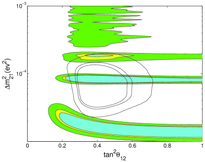
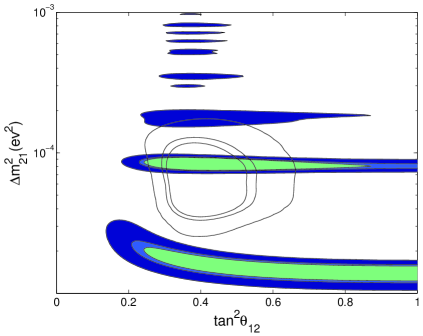
Using this expression, we obtained, in the $\tan^{2}\!\theta_{12}$–$\Delta{m}^{2}_{21}$ plane, the credible regions with 90%, 95% and 99.73% posterior probability shown in Fig. 1.

Figure 1: The 90%, 95%, 99.73% Bayesian credible regions in the $\tan^{2}\!\theta_{12}$–$\Delta{m}^{2}_{21}$ plane. Left: the regions allowed by the recent KamLAND 766 ton-years data (shadowed regions), together with the LMA region (empty contours) obtained from the analysis the solar neutrino data. Right: the region allowed by a combined analysis of solar and KamLAND neutrino data.

In our Bayesian analysis, a credible region is calculated by choosing the smallest region over which the integral of the posterior probability distribution function is the given probability level. For example, a 90% Bayesian credible region is the smallest region for which the posterior probability of the parameters is 90%.

Let us emphasize that the statistical meanings of Bayesian and Frequentist regions are different (see Refs. [31, 32, 33, 34, 35, 36, 37, 38, 17]). Nevertheless, it is interesting to compare the allowed regions obtained with the Bayesian and least-squares methods, especially in view of the fact that many scientists (and most human beings) do not know the meaning of Frequentist allowed regions and tend to give them a probability content, as if they were Bayesian credible regions. Fig. 2 shows a comparison of the Bayesian credible regions with 90%, 95% and 99.73% probability with the Frequentist allowed regions at 90%, 95% and 99.73% confidence level obtained with a least-squares analysis. One can see that the Bayesian credible regions are similar but a little larger than the corresponding allowed regions obtained with the least-squares analysis.

Differences between Bayesian credible regions and the corresponding Frequentist allowed regions can be due to a poor statistical quality of the data or to a wrong theoretical model which leads to a bad fit of the data. The close similarity of the Bayesian credible regions and the corresponding Frequentist allowed regions that we have obtained is a signal of the very good statistical quality of the data and a confirmation of the LMA solution of the solar neutrino problem. Note, however, that the similarity of the Bayesian and Frequentist results depends on the assumption of a flat prior in the Bayesian analysis. In section 5, we will change the prior probability distribution function in order to further test the stability of the LMA solution.

Figure 2: Comparisons of the Bayesian and least-squares methods. Going from left to right, the three figures correspond to 90%, 99% and 99.73% probability (Bayesian) or confidence level (least-squares).

It is also useful to calculate the marginal posterior probability distributions of $\tan^{2}\!\theta_{12}$ and $\Delta{m}^{2}_{21}$, which are given by

$$p(\tan^{2}\!\theta_{12}|\mathrm{D},\mathcal{I})=\int\mathrm{d}\Delta{m}^{2}_{21}\,p(\tan^{2}\!\theta_{12},\Delta{m}^{2}_{21}|\mathrm{D},\mathcal{I})\,,$$ (16)

$$p(\Delta{m}^{2}_{21}|\mathrm{D},\mathcal{I})=\int\mathrm{d}\!\tan^{2}\!\theta_{12}\,p(\tan^{2}\!\theta_{12},\Delta{m}^{2}_{21}|\mathrm{D},\mathcal{I})\,.$$ (17)

These distributions give information on each of the two parameters independently from the value of the other.

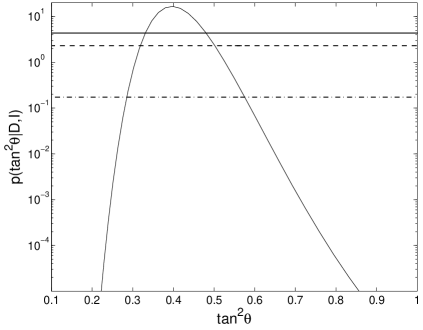
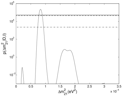
The marginal posterior probability distributions corresponding to the credible regions in Fig. 1 are shown in Fig. 3.

The marginal posterior probability distribution for $\tan^{2}\!\theta_{12}$, which is mainly determined by solar data, has only one peak with an approximate skewed-Gaussian shape. The resulting value of $\tan^{2}\!\theta_{12}$ is

$$\tan^{2}\!\theta_{12}=0.40{}^{+0.04}_{-0.04}\quad\text{(68\% probability range)}\,.$$ (18)

The allowed intervals with 90%, 95% and 99.73% probability, each of which is given by the intersections of the distribution function with the corresponding horizontal line in the left panel of Fig. 3, are

$$\tan^{2}\!\theta_{12}=[0.33\,,\,0.48]\,(90\%)\,,\quad[0.32\,,\,0.50]\,(95\%)\,,\quad[0.29\,,\,0.57]\,(99.73\%)\,.$$ (19)

The marginal posterior probability distribution for $\Delta{m}^{2}_{21}$ has one main peak and two small peaks on the sides. These two minor peaks correspond to the regions in the left panel of Fig. 1 which are allowed by the KamLAND data and have a partial overlap with the solar allowed region. However, from the right panel in Fig. 3, one can see that they are strongly disfavored with respect to the main peak, which gives

$$\Delta{m}^{2}_{21}=8.32{}^{+0.29}_{-0.30}\times 10^{-5}\,\text{eV}^{2}\quad\text{(68\% probability range)}\,.$$ (20)

The allowed intervals with 90%, 95% and 99.73% probability are

$$\Delta{m}^{2}_{21}=[7.76\,,\,8.89]\,(90\%)\,,\quad[7.73\,,\,8.91]\,(95\%)\,,\quad[7.37\,,\,9.32]\,(99.73\%)\quad\times 10^{-5}\text{eV}^{2}\,.$$ (21)

Figure 3: The marginal Bayesian distributions: left figure is a separated posterior probability distribution for $\tan^{2}\!\theta_{12}$; right figure is the separated posterior probability distributions for $\Delta{m}^{2}_{21}$. Three horizontal lines in each figure show three integrated probabilities: 90%, 95% and 99.73%(from up to down respectively).

Let us emphasize that the remarkable precision of the determination of $\tan^{2}\!\theta_{12}$ and $\Delta{m}^{2}_{21}$ in Eqs. (18)–(21) represents an impressive success of the solar and KamLAND neutrino experiments.

5 Stability of the LMA region

The Bayes’ Theorem in Eq. (11) requires a prior probability distribution function. The flat prior that we have adopted in the previous section is often considered as the best non-informative choice. In this section, we explore the implications for the Bayesian credible regions of different choices for the prior distribution, which may quantify some prior belief or knowledge.

From theoretical considerations, it is know that flavor transitions of solar neutrinos can occur over several orders of magnitude of $\tan^{2}\!\theta_{12}$ and $\Delta{m}^{2}_{21}$, through vacuum oscillations for $\Delta{m}^{2}_{21}\lesssim 10^{-8}\,\text{eV}^{2}$ and large mixing angles or resonant MSW transitions for $10^{-8}\,\text{eV}^{2}\lesssim\Delta{m}^{2}_{21}\lesssim 10^{-3}\,\text{eV}^{2}$ and $10^{-4}\lesssim\tan^{2}\!\theta_{12}\lesssim 10$. Hence, one may think that a flat prior distribution in the $\log(\tan^{2}\!\theta_{12})$–$\log(\Delta{m}^{2}_{21})$ plane,

$$p(\log(\tan^{2}\!\theta_{12}),\log(\Delta{m}^{2}_{21})|\mathcal{I})=\mathrm{const}\,,$$ (22)

is more appropriate than the flat prior distribution in the $\tan^{2}\!\theta_{12}$–$\Delta{m}^{2}_{21}$ plane in Eq. (14). In fact, this prior was adopted in Refs. [17, 21, 22]. In the $\tan^{2}\!\theta_{12}$–$\Delta{m}^{2}_{21}$ plane, it roughly corresponds to the prior

$$p(\tan^{2}\!\theta_{12},\Delta{m}^{2}_{21}|\mathcal{I})\propto\frac{1}{\tan^{2}\!\theta_{12}\,\Delta{m}^{2}_{21}}\,.$$ (23)

Slight differences between Eq. 22 and Eq. 23 is that in the $\tan^{2}\!\theta_{12}$–$\Delta{m}^{2}_{21}$ plane the credible region by Eq. 22 is no more iso contours and the probability at the center is shifted from the biggest value, and vise versa.

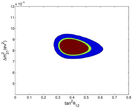
Fig. 4 shows the credible regions with 90%, 95% and 99.73% posterior probability obtained with the prior in Eq. (22). One can see that they are rather similar to the ones in Fig. 1, which have been obtained with the prior in Eq. (14), except for a slight preference of small values of the parameters due to the prior. However, a comparison of the right panels in Figs. 1 and 4 leads to the conclusion that the data are so good that the priors in Eqs. (14) and (23) produce almost the same result for the credible regions. Hence, in practice the choice between the priors in Eqs. (14) and (23) is irrelevant.

Figure 4: The 90%, 95%, 99.73% Bayesian credible regions in the $\log(\tan^{2}\!\theta_{12})$–$\log(\Delta{m}^{2}_{21})$ plane obtained with the prior in Eq. (22). Left: the regions allowed by the KamLAND 766 ton-years data (shadowed regions), together with the LMA region (empty contours) obtained from the analysis the solar neutrino data. Right: the region allowed by a combined analysis of solar and KamLAND neutrino data.

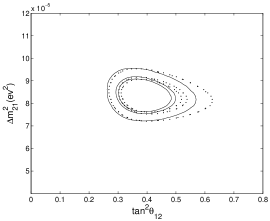
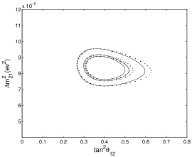
We consider now a prior which is a flat distribution with respect to $\Delta{m}^{2}_{21}$ and a normal distribution for the parameter $\tan^{2}\!\theta_{12}$:

$$p(\tan^{2}\!\theta_{12},\Delta{m}^{2}_{21}|\mathcal{I})=\frac{1}{\sqrt{2\pi}\sigma}\,e^{-(\tan^{2}\theta_{12}-\mu)^{2}/2\sigma^{2}}\,.$$ (24)

This case corresponds to a prior belief in $\tan^{2}\!\theta_{12}\simeq\mu$, with an uncertainty $\sigma$. The Bayes’ Theorem in Eq. (11) gives the posterior probability distribution

$$p(\tan^{2}\!\theta_{12},\Delta{m}^{2}_{21}|\mathrm{D},\mathcal{I})=\frac{\displaystyle p(\mathrm{D}|\tan^{2}\!\theta_{12},\Delta{m}^{2}_{21},\mathcal{I})\,e^{-(\tan^{2}\theta_{12}-\mu)^{2}/2\sigma^{2}}}{\displaystyle\int\mathrm{d}\!\tan^{2}\!\theta_{12}\,\mathrm{d}\Delta{m}^{2}_{21}\,p(\mathrm{D}|\tan^{2}\!\theta_{12},\Delta{m}^{2}_{21},\mathcal{I})\,e^{-(\tan^{2}\theta_{12}-\mu)^{2}/2\sigma^{2}}}\,.$$ (25)

Figure 5: The 90%, 95%, and 99.73% credible regions corresponding to the posterior probability distribution function in Eq. (25), with $\mu=0$. The left, middle and right figures have been obtained, respectively, with $\sigma=0.2$, $0.3$, and $0.5$. The dotted lines correspond to a flat prior distribution (same as the right figure in Fig. 1).

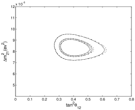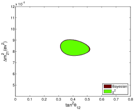
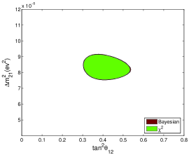
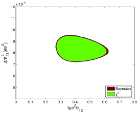
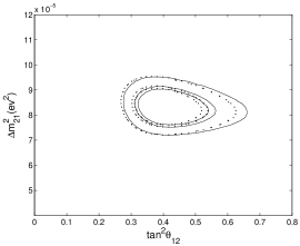
Fig. 5 shows the 90%, 95%, and 99.73% credible regions for $\mu=0$ and $\sigma=0.2,0.3,0.5$. The value $\mu=0$ corresponds to a prior belief that the mixing angle should be small. One can see from the three panels in Fig. 5 that a small value of $\sigma$ has the effect to exclude the large-$\tan^{2}\theta_{12}$ part of the credible regions obtained with a flat prior in section 4. On the other hand, the low-$\tan^{2}\theta_{12}$ part of the credible regions is not affected by the change of prior. This is due to the KamLAND data, which exclude small values of $\tan^{2}\theta_{12}$, as shown in the left panel of Fig. 1.

Figure 6: The 90%, 95%, and 99.73% credible regions corresponding to the posterior probability distribution function in Eq. (25), with $\mu=1$. The left, middle and right figures have been obtained, respectively, with $\sigma=0.2$, $0.3$, and $0.5$. The dotted lines correspond to a flat prior distribution (same as the right figure in Fig. 1).

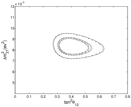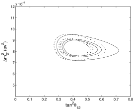
Figs. 6 shows the 90%, 95%, and 99.73% credible regions for $\mu=1$ and $\sigma=0.2,0.3,0.5$. The value $\mu=1$ corresponds to a prior belief in favor of a large mixing angle, close to maximal. The leftmost panel in Fig. 6 shows that, with respect to the case of a flat prior considered in section 4, a small value of $\sigma$ leads to an enlargement of the credible regions towards large values of $\tan^{2}\theta_{12}$, which are allowed by the KamLAND data, as shown in the left panel of Fig. 1. The low-$\tan^{2}\theta_{12}$ part of the credible regions is affected only mildly by the change of prior.

In conclusion, in this section we have shown that the LMA solution is stable when reasonable priors are chosen in place of the flat one considered in section 4, with a possible shrink or enlargement of the large-$\tan^{2}\theta_{12}$ part of the credible regions depending on a prior belief in favor of a small or large mixing angle.

6 Conclusions

In this paper, we presented the results of a Bayesian analysis of the solar and KamLAND neutrino data. We showed that the Bayesian analysis with a flat prior distribution in the $\tan^{2}\!\theta_{12}$–$\Delta{m}^{2}_{21}$ plane leads to an allowed LMA region for $\nu_{e}\to\nu_{\mu,\tau}$ transitions which practically coincides with the one obtained with a standard least-squares ($\chi^{2}$) analysis. We investigated the stability of the LMA allowed region for other reasonable choices of the prior. We have shown that the LMA solution is stable against reasonable variations of the prior, with a possible shrink or enlargement of the large-$\tan^{2}\theta_{12}$ part of the allowed LMA region if one has a prior belief, respectively, in favor of a small or large mixing angle.

7 Acknowledgments

The authors from USTC would like to thank M.J. Luo and Y.F. Li for useful discussions. This work is supported in part by the National Natural Science Foundation of China under grant number 90203002.

References

- [1] B. T. Cleveland et al., Astrophys. J. 496, 505 (1998); K. Lande, Talk given at the Neutrino ’96 Int. Conference, June 13 - 19, 1996, Helsinki, Finland; see also: R. Davis, Prog. Part. Nucl. Phys. 32, 13 (1994); B. T. Cleveland et al., Nucl. Phys. B (Proc. Suppl.) 38, 47 (1995).
- [2] K.S. Hirata, et al., Phys. Rev. D 44, 2241 (1991); K.S. Hirata, et al., Phys. Rev. Lett. 66, 9 (1991); Y. Fukuda et al., Phys. Rev. Lett. 77, 1683 (1996).
- [3] M. Altmann et al., Phys. Lett. B 616, 174 (2005), hep-ex/0504037]; P. Anselmann et al., Phys. Lett. B 357, 237 (1995) (see also: ibid. B 327, 377 (1994)).
- [4] J. N. Abdurashitov et al., J. Exp. Theor. Phys. 95, 181 (2002), astro-ph/0204245; V. Gavrin et al., Talk given at the Neutrino ’96 Int. Conference, June 13 - 19, 1996, Helsinki, Finland; J. N. Abdurashitov et al., Phys. Lett. B 328, 234 (1994).
- [5] J. Hosaka et al., hep-ex/0508053; M. B. Smy et al., Phys. Rev. D 69, 011104 (2004), hep-ex/0309011; S. Fukuda et al., Phys. Lett. B 539, 179 (2002), hep-ex/0205075.
- [6] Q. R. Ahmad et al., Phys. Rev. Lett. 87, 071301 (2001), nucl-ex/0106015; Phys. Rev. Lett. 89, 011302 (2002), nucl-ex/0204009.
- [7] Q. R. Ahmad et al., Phys. Rev. Lett. 89, 011301 (2002), nucl-ex/0204008.
- [8] S. N. Ahmed et al., Phys. Rev. Lett. 92, 181301 (2004), nucl-ex/0309004.
- [9] B. Aharmim et al. [SNO Collaboration], Phys. Rev. C 72, 055502 (2005), nucl-ex/0502021.
- [10] S.P. Mikheyev and A.Yu. Smirnov, Yad. Fiz., 42, 1441 (1985); L. Wolfenstein, Phys. Rev. D17, 2369 (1978).
- [11] A. Suzuki, talk at the XVIII International Conference on Neutrino Physics and Astrophysics, Takayama, Japan, (1998); K. Eguchi et al. [KamLAND Collaboration], Phys. Rev. Lett. 90, 021802 (2003); T. Araki et al. [KamLAND Collaboration], Phys. Rev. Lett. 94, 081801 (2005).
- [12] S. M. Bilenky, C. Giunti and W. Grimus, Prog. Part. Nucl. Phys. 43, 1 (1999), hep-ph/9812360.
- [13] C. Giunti, “Neutrino Physics”, Lectures at Salerno University, Italy, 24-28 April 2006, http://www.nu.to.infn.it/pap/2006/giunti-2006-salerno.pdf”.
- [14] J. Hosaka et al., hep-ex/0604011.
- [15] Q.Y. Liu, B.L. Chen, J. Zhou, M.J. Luo, S.C. Jing, Theor. Phys.(Beijing, China) 44, 505 (2005).
- [16] Q.Y. Liu and S.T. Petcov, Phys. Rev. D 56, 7392 (1997); Q.Y. Liu, proceedings of 4th International Solar Neutrino Conference, Heidelberg, Germany, (1997) hep-ph/9708308, K.S. Babu, Q.Y. Liu and A.Yu. Smirnov, Phys. Rev. D 57, 5825 (1998), hep-ph/9707457.
- [17] M. V. Garzelli and C. Giunti, JHEP 0112, 017 (2001), hep-ph/0108191.
- [18] F. James, in Advanced Statistical Techniques In Particle Physics, edited by M.R. Whalley and L. Lyons. Durham, UK, Inst. For Particle Physics Phenomenology, 2002, http://www.ippp.dur.ac.uk/Workshops/02/statistics/.
- [19] C. Giunti, in Advanced Statistical Techniques In Particle Physics, edited by M.R. Whalley and L. Lyons. Durham, UK, Inst. For Particle Physics Phenomenology, 2002, http://www.ippp.dur.ac.uk/Workshops/02/statistics/.
- [20] C. M. Bhat, P. C. Bhat, M. Paterno and H. B. Prosper, Phys. Rev. Lett. 81, 5056 (1998), astro-ph/9804252; H. B. Prosper, hep-ph/0006356, Yellow Report CERN 2000-005, pp. 29–47. Workshop on Confidence Limits, CERN, 17-18 January 2000.
- [21] P. Creminelli, G. Signorelli and A. Strumia, JHEP 0105, 052 (2001), hep-ph/0102234.
- [22] M. V. Garzelli and C. Giunti, Phys. Rev. D 65, 093005 (2002), hep-ph/0111254.
- [23] P.C.de Holanda and A.Yu.Smirnov, Phys. Rev. D 66, 113005 (2002), hep-ph/0205241.
- [24] P.C. de Holanda and A. Yu. Smirnov, J. Cosmol. Astropart. Phys. 02, 001 (2003).
- [25] J. N. Bahcall, M. C. Gonzalez-Garcia and C. Pea-Garay, High Energy Phys. 02, 009 (2003).
- [26] J. N. Bahcall and M. H. Pinsonneault, Phys. Rev. Lett. 92 (2004) 121301, astro-ph/0402114.
- [27] G. L. Fogli and E. Lisi, Astropart. Phys. 3, 185 (1995).
- [28] G. L. Fogli, E. Lisi, D. Montanino and A. Palazzo, Phys. Rev. D 62, 013002 (2000), hep-ph/9912231.
- [29] M. V. Garzelli and C. Giunti, Phys. Lett. B 488, 339 (2000), hep-ph/0006026.
- [30] K. Hagiwara et al. [Particle Data Group Collaboration], Phys. Rev. D 66, 010001 (2002).
- [31] H. Jeffreys, Theory of Probability, Oxford University Press, New York, USA, 1961. First published in 1939.
- [32] W.T. Eadie, D. Drijard, F.E. James, M. Roos and B. Sadoulet, Statistical Methods in Experimental Physics, North Holland, Amsterdam, 1971.
- [33] A. Stuart, J.K. Ord and S. Arnold, Kendall’s Advanced Theory of Statistics, Vol. 2A, Classical Inference & the Linear Model, Sixth Edition, Halsted Press, 1999.
- [34] T. J. Loredo, in Maximum-Entropy and Bayesian Methods, Dartmouth, 1989, pp. 81–142, http://astrosun.tn.cornell.edu/staff/loredo/bayes/tjl.html.
- [35] T. J. Loredo, in Statistical Challenges in Modern Astronomy, Springer-Verlag, New York, 1992, pp. 275–297, http://astrosun.tn.cornell.edu/staff/loredo/bayes/tjl.html.
- [36] E. T. Jaynes, Probability Theory: The Logic of Science, Cambridge University Press, 2003.
- [37] G. D’Agostini, Bayesian Reasoning in Data Analysis, A Critical Introduction, World Scientific, 2003.
- [38] M. V. Garzelli and C. Giunti, Astropart. Phys. 17, 205 (2002), hep-ph/0007155.