Probing anomalous W​t​bπ‘Šπ‘‘π‘\boldsymbol{Wtb} couplings in top pair decays

J. A. Aguilar–Saavedraa, J. Carvalhob, N. Castrob, A. Onofreb,c, F. Velosob

a Departamento de F sica Te rica y del Cosmos and CAFPE,
Universidad de Granada, E-18071 Granada, Spain

b LIP - Departamento de F sica,
Universidade de Coimbra, 3004-516 Coimbra, Portugal

c UCP, Rua Dr. Mendes Pinheiro 24, 3080 Figueira da Foz, Portugal

Abstract

We investigate several quantities, defined in the decays of top quark pairs, which can be used to explore non-standard W​t​bπ‘Šπ‘‘π‘Wtb interactions. Two new angular asymmetries are introduced in the leptonic decay of top (anti)quarks. Both are very sensitive to anomalous W​t​bπ‘Šπ‘‘π‘Wtb couplings, and their measurement allows for a precise determination of the Wπ‘ŠW helicity fractions. We also examine other angular and energy asymmetries, the Wπ‘ŠW helicity fractions and their ratios, as well as spin correlation asymmetries, analysing their dependence on anomalous W​t​bπ‘Šπ‘‘π‘Wtb couplings and identifing the quantities which are most sensitive to them. It is explicitly shown that spin correlation asymmetries are less sensitive to new interactions in the decay of the top quark; therefore, when combined with the measurement of other observables, they can be used to determine the t​t¯𝑑¯𝑑t\bar{t} spin correlation even in the presence of anomalous W​t​bπ‘Šπ‘‘π‘Wtb couplings. We finally discuss some asymmetries which can be used to test CP violation in t​t¯𝑑¯𝑑t\bar{t} production and complex phases in the effective W​t​bπ‘Šπ‘‘π‘Wtb vertex.

1 Introduction

Precision studies have been in the past a powerful tool to explore new physics at scales not kinematically accessible. With the operation of the Large Hadron Collider (LHC), top physics will enter into the era of precise measurements [1]. Due to its large mass, close to the electroweak scale, the top quark is believed to offer a unique window to physics beyond the Standard Model (SM). New interactions at higher energies may manifest themselves in the form of effective couplings of the SM fermions, especially for the top quark, much heavier than the rest. In this work we concentrate ourselves on the W​t​bπ‘Šπ‘‘π‘Wtb vertex. Within the SM this coupling is purely left-handed, and its size is given by the Cabibbo-Kobayashi-Maskawa matrix element Vt​bsubscript𝑉𝑑𝑏V_{tb}, which can be measured in single top production [2, 3, 4]. In new physics models, departures from the SM expectation Vt​b≃1similar-to-or-equalssubscript𝑉𝑑𝑏1V_{tb}\simeq 1 are possible [5, 6], as well as new radiative contributions to the W​t​bπ‘Šπ‘‘π‘Wtb vertex [7, 8]. These corrections can be parameterised with the effective operator formalism. The most general W​t​bπ‘Šπ‘‘π‘Wtb vertex containing terms up to dimension five can be written as

β„’β„’\displaystyle\mathcal{L} =\displaystyle= βˆ’g2​b¯​γμ​(VL​PL+VR​PR)​t​WΞΌβˆ’π‘”2¯𝑏superscriptπ›Ύπœ‡subscript𝑉𝐿subscript𝑃𝐿subscript𝑉𝑅subscript𝑃𝑅𝑑superscriptsubscriptπ‘Šπœ‡\displaystyle-\frac{g}{\sqrt{2}}\bar{b}\,\gamma^{\mu}\left(V_{L}P_{L}+V_{R}P_{R}\right)t\;W_{\mu}^{-} (1)
βˆ’g2​b¯​i​σμ​ν​qΞ½MW​(gL​PL+gR​PR)​t​WΞΌβˆ’+h.c.,formulae-sequence𝑔2¯𝑏𝑖superscriptπœŽπœ‡πœˆsubscriptπ‘žπœˆsubscriptπ‘€π‘Šsubscript𝑔𝐿subscript𝑃𝐿subscript𝑔𝑅subscript𝑃𝑅𝑑superscriptsubscriptπ‘Šπœ‡hc\displaystyle-\frac{g}{\sqrt{2}}\bar{b}\,\frac{i\sigma^{\mu\nu}q_{\nu}}{M_{W}}\left(g_{L}P_{L}+g_{R}P_{R}\right)t\;W_{\mu}^{-}+\mathrm{h.c.}\,,

with q=ptβˆ’pbπ‘žsubscript𝑝𝑑subscript𝑝𝑏q=p_{t}-p_{b} (we follow the conventions of Ref.Β [9] with slight simplifications in the notation). If CP is conserved in the decay, the couplings can be taken to be real.111A general W​t​bπ‘Šπ‘‘π‘Wtb vertex also contains terms proportional to (pt+pb)ΞΌsuperscriptsubscript𝑝𝑑subscriptπ‘π‘πœ‡(p_{t}+p_{b})^{\mu}, qΞΌsuperscriptπ‘žπœ‡q^{\mu} and σμ​ν​(pt+pb)Ξ½superscriptπœŽπœ‡πœˆsubscriptsubscript𝑝𝑑subscriptπ‘π‘πœˆ\sigma^{\mu\nu}(p_{t}+p_{b})_{\nu}. Since b𝑏b quarks are on shell, the Wπ‘ŠW bosons decay to light particles (whose masses can be neglected) and the top quarks can be approximately assumed on-shell, these extra operators can be rewritten in terms of the ones in Eq.Β (1) using Gordon identities. Within the SM, VL≑Vt​b≃1subscript𝑉𝐿subscript𝑉𝑑𝑏similar-to-or-equals1V_{L}\equiv V_{tb}\simeq 1 and VRsubscript𝑉𝑅V_{R}, gLsubscript𝑔𝐿g_{L}, gRsubscript𝑔𝑅g_{R} vanish at the tree level, while nonzero values are generated at one loop level [10]. Additional contributions to VRsubscript𝑉𝑅V_{R}, gLsubscript𝑔𝐿g_{L}, gRsubscript𝑔𝑅g_{R} are possible in SM extensions, without spoiling the agreement with low-energy measurements. The size of a VRsubscript𝑉𝑅V_{R} term is constrained by the measured rate of Br​(bβ†’s​γ)=(3.3Β±0.4)Γ—10βˆ’4Br→𝑏𝑠𝛾plus-or-minus3.30.4superscript104\mathrm{Br}(b\to s\gamma)=(3.3\pm 0.4)\times 10^{-4} [11]. A right-handed coupling |VR|≳0.04greater-than-or-equivalent-tosubscript𝑉𝑅0.04|V_{R}|\gtrsim 0.04 would in principle give a too large contribution to this decay [12] which, however, might be (partially) cancelled with other new physics contributions. Hence, the bound |VR|≀0.04subscript𝑉𝑅0.04|V_{R}|\leq 0.04 is model dependent and does not substitute a direct measurement of this coupling. Similar arguments applied to the σμ​νsuperscriptπœŽπœ‡πœˆ\sigma^{\mu\nu} terms do not set relevant constraints on gRsubscript𝑔𝑅g_{R}, because its contribution is suppressed by the ratio qΞ½/MWsubscriptπ‘žπœˆsubscriptπ‘€π‘Šq_{\nu}/M_{W} for small qΞ½subscriptπ‘žπœˆq_{\nu}.

Top production and decay processes at LHC allow us to probe the W​t​bπ‘Šπ‘‘π‘Wtb vertex [2, 4, 9, 13, 14]. Top pair production takes place through QCD interactions without involving a W​t​bπ‘Šπ‘‘π‘Wtb coupling. Additionally, it is likely that the top quark almost exclusively decays in the channel tβ†’W+​b→𝑑superscriptπ‘Šπ‘t\to W^{+}b. Therefore, its cross section for production and decay g​g,q​qΒ―β†’t​tΒ―β†’W+​b​Wβˆ’β€‹bΒ―β†’π‘”π‘”π‘žΒ―π‘žπ‘‘Β―π‘‘β†’superscriptπ‘Šπ‘superscriptπ‘ŠΒ―π‘gg,q\bar{q}\to t\bar{t}\to W^{+}bW^{-}\bar{b} is insensitive to the size and structure of the W​t​bπ‘Šπ‘‘π‘Wtb vertex. However, the angular distributions of (anti)top decay products give information about its structure, and can then be used to trace non-standard couplings. Angular distributions relating top and antitop decay products probe not only the W​t​bπ‘Šπ‘‘π‘Wtb interactions but also the spin correlations among the two quarks produced, and thus may be influenced by new production mechanisms as well. On the other hand, single top production is sensitive to both the size and structure of the W​t​bπ‘Šπ‘‘π‘Wtb vertex, involved in the production and the decay of the top quark [4, 13, 14].

In this paper we explore the sensitivity of several quantities, like angular and energy asymmetries, helicity fractions and ratios, to new non-standard W​t​bπ‘Šπ‘‘π‘Wtb interactions. Although these observables are theoretically related, the experimental determination is more precise for some of them than for others. In particular, the experimental precision is dominated by systematics already for a luminosity of 10 fb-1, and a good choice of observables can improve significantly the limits on anomalous W​t​bπ‘Šπ‘‘π‘Wtb interactions. Our analysis here is kept at a purely theoretical level, identifying the quantities which are a priori more sensitive to anomalous couplings, and estimating the precision in their experimental measurement from a detailed simulation, which has been presented elsewhere [15, 16].

2 𝑾𝑾\boldsymbol{W} helicity fractions and ratios

The polarisation of the Wπ‘ŠW bosons emitted in the top decay is sensitive to non-standard couplings [17]. The Wπ‘ŠW bosons can be produced with positive (right-handed), negative (left-handed) or zero helicity, with corresponding partial widths Ξ“RsubscriptΓ𝑅\Gamma_{R}, Ξ“LsubscriptΓ𝐿\Gamma_{L}, Ξ“0subscriptΞ“0\Gamma_{0}, being Γ≑Γ​(tβ†’W+​b)=Ξ“R+Ξ“L+Ξ“0ΓΓ→𝑑superscriptπ‘Šπ‘subscriptΓ𝑅subscriptΓ𝐿subscriptΞ“0\Gamma\equiv\Gamma(t\to W^{+}b)=\Gamma_{R}+\Gamma_{L}+\Gamma_{0}. The Ξ“RsubscriptΓ𝑅\Gamma_{R} component vanishes in the mb=0subscriptπ‘šπ‘0m_{b}=0 limit because the b𝑏b quarks produced in top decays have left-handed chirality, and for vanishing mbsubscriptπ‘šπ‘m_{b} the helicity and the chirality states coincide. The three partial widths can be calculated for a general W​t​bπ‘Šπ‘‘π‘Wtb vertex as parameterised in Eq.Β (1), yielding

Ξ“0subscriptΞ“0\displaystyle\Gamma_{0} =\displaystyle= g2​|qβ†’|32​π{mt2MW2[|VL|2+|VR|2](1βˆ’xW2βˆ’2xb2βˆ’xW2xb2+xb4)βˆ’4xbReVLVRβˆ—\displaystyle\frac{g^{2}|\vec{q}\,|}{32\pi}\left\{\frac{m_{t}^{2}}{M_{W}^{2}}\left[|V_{L}|^{2}+|V_{R}|^{2}\right]\left(1-x_{W}^{2}-2x_{b}^{2}-x_{W}^{2}x_{b}^{2}+x_{b}^{4}\right)-4x_{b}\,\text{Re}\,V_{L}V_{R}^{*}\right.
+[|gL|2+|gR|2]​(1βˆ’xW2+xb2)βˆ’4​xb​Re​gL​gRβˆ—delimited-[]superscriptsubscript𝑔𝐿2superscriptsubscript𝑔𝑅21superscriptsubscriptπ‘₯π‘Š2superscriptsubscriptπ‘₯𝑏24subscriptπ‘₯𝑏Resubscript𝑔𝐿superscriptsubscript𝑔𝑅\displaystyle+\left[|g_{L}|^{2}+|g_{R}|^{2}\right]\left(1-x_{W}^{2}+x_{b}^{2}\right)-4x_{b}\,\text{Re}\,g_{L}g_{R}^{*}
βˆ’2​mtMW​Re​[VL​gRβˆ—+VR​gLβˆ—]​(1βˆ’xW2βˆ’xb2)2subscriptπ‘šπ‘‘subscriptπ‘€π‘ŠRedelimited-[]subscript𝑉𝐿superscriptsubscript𝑔𝑅subscript𝑉𝑅superscriptsubscript𝑔𝐿1superscriptsubscriptπ‘₯π‘Š2superscriptsubscriptπ‘₯𝑏2\displaystyle-2\frac{m_{t}}{M_{W}}\text{Re}\,\left[V_{L}g_{R}^{*}+V_{R}g_{L}^{*}\right]\left(1-x_{W}^{2}-x_{b}^{2}\right)
+2mtMWxbRe[VLgLβˆ—+VRgRβˆ—](1+xW2βˆ’xb2)},\displaystyle\left.+2\frac{m_{t}}{M_{W}}x_{b}\,\text{Re}\,\left[V_{L}g_{L}^{*}+V_{R}g_{R}^{*}\right]\left(1+x_{W}^{2}-x_{b}^{2}\right)\right\}\,,
Ξ“R,LsubscriptΓ𝑅𝐿\displaystyle\Gamma_{R,L} =\displaystyle= g2​|qβ†’|32​π{[|VL|2+|VR|2](1βˆ’xW2+xb2)βˆ’4xbReVLVRβˆ—\displaystyle\frac{g^{2}|\vec{q}\,|}{32\pi}\left\{\left[|V_{L}|^{2}+|V_{R}|^{2}\right]\left(1-x_{W}^{2}+x_{b}^{2}\right)-4x_{b}\,\text{Re}\,V_{L}V_{R}^{*}\right. (2)
+mt2MW2​[|gL|2+|gR|2]​(1βˆ’xW2βˆ’2​xb2βˆ’xW2​xb2+xb4)βˆ’4​xb​Re​gL​gRβˆ—superscriptsubscriptπ‘šπ‘‘2superscriptsubscriptπ‘€π‘Š2delimited-[]superscriptsubscript𝑔𝐿2superscriptsubscript𝑔𝑅21superscriptsubscriptπ‘₯π‘Š22superscriptsubscriptπ‘₯𝑏2superscriptsubscriptπ‘₯π‘Š2superscriptsubscriptπ‘₯𝑏2superscriptsubscriptπ‘₯𝑏44subscriptπ‘₯𝑏Resubscript𝑔𝐿superscriptsubscript𝑔𝑅\displaystyle+\frac{m_{t}^{2}}{M_{W}^{2}}\left[|g_{L}|^{2}+|g_{R}|^{2}\right]\left(1-x_{W}^{2}-2x_{b}^{2}-x_{W}^{2}x_{b}^{2}+x_{b}^{4}\right)-4x_{b}\,\text{Re}\,g_{L}g_{R}^{*}
βˆ’2​mtMW​Re​[VL​gRβˆ—+VR​gLβˆ—]​(1βˆ’xW2βˆ’xb2)2subscriptπ‘šπ‘‘subscriptπ‘€π‘ŠRedelimited-[]subscript𝑉𝐿superscriptsubscript𝑔𝑅subscript𝑉𝑅superscriptsubscript𝑔𝐿1superscriptsubscriptπ‘₯π‘Š2superscriptsubscriptπ‘₯𝑏2\displaystyle-2\frac{m_{t}}{M_{W}}\text{Re}\,\left[V_{L}g_{R}^{*}+V_{R}g_{L}^{*}\right]\left(1-x_{W}^{2}-x_{b}^{2}\right)
+2mtMWxbRe[VLgLβˆ—+VRgRβˆ—](1+xW2βˆ’xb2)}\displaystyle\left.+2\frac{m_{t}}{M_{W}}x_{b}\,\text{Re}\,\left[V_{L}g_{L}^{*}+V_{R}g_{R}^{*}\right]\left(1+x_{W}^{2}-x_{b}^{2}\right)\right\}
Β±g264​πmt3MW2{βˆ’xW2[|VL|2βˆ’|VR|2]+[|gL|2βˆ’|gR|2](1βˆ’xb2)\displaystyle\pm\frac{g^{2}}{64\pi}\frac{m_{t}^{3}}{M_{W}^{2}}\left\{-x_{W}^{2}\left[|V_{L}|^{2}-|V_{R}|^{2}\right]+\left[|g_{L}|^{2}-|g_{R}|^{2}\right]\left(1-x_{b}^{2}\right)\right.
+2xWRe[VLgRβˆ—βˆ’VRgLβˆ—]+2xWxbRe[VLgLβˆ—βˆ’VRgRβˆ—]}\displaystyle\left.+2x_{W}\,\text{Re}\,\left[V_{L}g_{R}^{*}-V_{R}g_{L}^{*}\right]+2x_{W}x_{b}\,\text{Re}\,\left[V_{L}g_{L}^{*}-V_{R}g_{R}^{*}\right]\right\}
Γ—(1βˆ’2​xW2βˆ’2​xb2+xW4βˆ’2​xW2​xb2+xb4),absent12superscriptsubscriptπ‘₯π‘Š22superscriptsubscriptπ‘₯𝑏2superscriptsubscriptπ‘₯π‘Š42superscriptsubscriptπ‘₯π‘Š2superscriptsubscriptπ‘₯𝑏2superscriptsubscriptπ‘₯𝑏4\displaystyle\times\left(1-2x_{W}^{2}-2x_{b}^{2}+x_{W}^{4}-2x_{W}^{2}x_{b}^{2}+x_{b}^{4}\right)\,,

being xW=MW/mtsubscriptπ‘₯π‘Šsubscriptπ‘€π‘Šsubscriptπ‘šπ‘‘x_{W}=M_{W}/m_{t}, xb=mb/mtsubscriptπ‘₯𝑏subscriptπ‘šπ‘subscriptπ‘šπ‘‘x_{b}=m_{b}/m_{t} and

|qβ†’|=12​mt​(mt4+MW4+mb4βˆ’2​mt2​MW2βˆ’2​mt2​mb2βˆ’2​MW2​mb2)1/2β†’π‘ž12subscriptπ‘šπ‘‘superscriptsuperscriptsubscriptπ‘šπ‘‘4superscriptsubscriptπ‘€π‘Š4superscriptsubscriptπ‘šπ‘42superscriptsubscriptπ‘šπ‘‘2superscriptsubscriptπ‘€π‘Š22superscriptsubscriptπ‘šπ‘‘2superscriptsubscriptπ‘šπ‘22superscriptsubscriptπ‘€π‘Š2superscriptsubscriptπ‘šπ‘212|\vec{q}\,|=\frac{1}{2m_{t}}(m_{t}^{4}+M_{W}^{4}+m_{b}^{4}-2m_{t}^{2}M_{W}^{2}-2m_{t}^{2}m_{b}^{2}-2M_{W}^{2}m_{b}^{2})^{1/2} (3)

the modulus of the Wπ‘ŠW boson three-momentum in the top quark rest frame. The total top width is

ΓΓ\displaystyle\Gamma =\displaystyle= g2​|qβ†’|32​πmt2MW2{[|VL|2+|VR|2](1+xW2βˆ’2xb2βˆ’2xW4+xW2xb2+xb4)\displaystyle\frac{g^{2}|\vec{q}\,|}{32\pi}\frac{m_{t}^{2}}{M_{W}^{2}}\left\{\left[|V_{L}|^{2}+|V_{R}|^{2}\right]\left(1+x_{W}^{2}-2x_{b}^{2}-2x_{W}^{4}+x_{W}^{2}x_{b}^{2}+x_{b}^{4}\right)\right. (4)
βˆ’12​xW2​xb​Re​VL​VRβˆ—+2​[|gL|2+|gR|2]​(1βˆ’xW22βˆ’2​xb2βˆ’xW42βˆ’xW2​xb22+xb4)12superscriptsubscriptπ‘₯π‘Š2subscriptπ‘₯𝑏Resubscript𝑉𝐿superscriptsubscript𝑉𝑅2delimited-[]superscriptsubscript𝑔𝐿2superscriptsubscript𝑔𝑅21superscriptsubscriptπ‘₯π‘Š222superscriptsubscriptπ‘₯𝑏2superscriptsubscriptπ‘₯π‘Š42superscriptsubscriptπ‘₯π‘Š2superscriptsubscriptπ‘₯𝑏22superscriptsubscriptπ‘₯𝑏4\displaystyle-12x_{W}^{2}x_{b}\,\text{Re}\,V_{L}V_{R}^{*}+2\left[|g_{L}|^{2}+|g_{R}|^{2}\right]\left(1-\frac{x_{W}^{2}}{2}-2x_{b}^{2}-\frac{x_{W}^{4}}{2}-\frac{x_{W}^{2}x_{b}^{2}}{2}+x_{b}^{4}\right)
βˆ’12​xW2​xb​Re​gL​gRβˆ—βˆ’6​xW​Re​[VL​gRβˆ—+VR​gLβˆ—]​(1βˆ’xW2βˆ’xb2)12superscriptsubscriptπ‘₯π‘Š2subscriptπ‘₯𝑏Resubscript𝑔𝐿superscriptsubscript𝑔𝑅6subscriptπ‘₯π‘ŠRedelimited-[]subscript𝑉𝐿superscriptsubscript𝑔𝑅subscript𝑉𝑅superscriptsubscript𝑔𝐿1superscriptsubscriptπ‘₯π‘Š2superscriptsubscriptπ‘₯𝑏2\displaystyle-12x_{W}^{2}x_{b}\,\text{Re}\,g_{L}g_{R}^{*}-6x_{W}\text{Re}\,\left[V_{L}g_{R}^{*}+V_{R}g_{L}^{*}\right]\left(1-x_{W}^{2}-x_{b}^{2}\right)
+6xWxbRe[VLgLβˆ—+VRgRβˆ—](1+xW2βˆ’xb2)}.\displaystyle\left.+6x_{W}x_{b}\,\text{Re}\,\left[V_{L}g_{L}^{*}+V_{R}g_{R}^{*}\right]\left(1+x_{W}^{2}-x_{b}^{2}\right)\right\}\,.

The different polarisation states of the Wπ‘ŠW boson are reflected in the angular distribution of its decay products. Let us denote by ΞΈβ„“βˆ—superscriptsubscriptπœƒβ„“\theta_{\ell}^{*} the angle between the charged lepton three-momentum in the Wπ‘ŠW rest frame and the Wπ‘ŠW momentum in the t𝑑t rest frame. The normalised differential decay rate for unpolarised top quarks can be written as

1Γ​d​Γd​cosβ‘ΞΈβ„“βˆ—=38​(1+cosβ‘ΞΈβ„“βˆ—)2​FR+38​(1βˆ’cosβ‘ΞΈβ„“βˆ—)2​FL+34​sin2β‘ΞΈβ„“βˆ—β€‹F0,1Γ𝑑Γ𝑑superscriptsubscriptπœƒβ„“38superscript1superscriptsubscriptπœƒβ„“2subscript𝐹𝑅38superscript1superscriptsubscriptπœƒβ„“2subscript𝐹𝐿34superscript2superscriptsubscriptπœƒβ„“subscript𝐹0\frac{1}{\Gamma}\frac{d\Gamma}{d\cos\theta_{\ell}^{*}}=\frac{3}{8}(1+\cos\theta_{\ell}^{*})^{2}\,F_{R}+\frac{3}{8}(1-\cos\theta_{\ell}^{*})^{2}\,F_{L}+\frac{3}{4}\sin^{2}\theta_{\ell}^{*}\,F_{0}\,, (5)

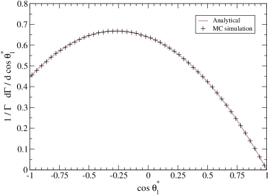
with Fi≑Γi/Ξ“subscript𝐹𝑖subscriptΓ𝑖ΓF_{i}\equiv\Gamma_{i}/\Gamma the helicity fractions. The three terms correspond to the three helicity states, and the interference terms vanish [18]. At the tree level, F0=0.703subscript𝐹00.703F_{0}=0.703, FL=0.297subscript𝐹𝐿0.297F_{L}=0.297, FR=3.6Γ—10βˆ’4subscript𝐹𝑅3.6superscript104F_{R}=3.6\times 10^{-4}, for mt=175subscriptπ‘šπ‘‘175m_{t}=175 GeV, MW=80.39subscriptπ‘€π‘Š80.39M_{W}=80.39 GeV, mb=4.8subscriptπ‘šπ‘4.8m_{b}=4.8 GeV. The resulting distribution is shown in Fig.Β 1, calculated from the analytical expressions in Eqs.Β (2)–(5) and also with a Monte Carlo simulation. The latter is performed using our own t​t¯𝑑¯𝑑t\bar{t} generator, which uses the full resonant matrix element for g​g,q​qΒ―β†’t​tΒ―β†’W+​b​Wβˆ’β€‹bΒ―β†’f1​fΒ―1′​b​fΒ―2​f2′​bΒ―β†’π‘”π‘”π‘žΒ―π‘žπ‘‘Β―π‘‘β†’superscriptπ‘Šπ‘superscriptπ‘ŠΒ―π‘β†’subscript𝑓1superscriptsubscript¯𝑓1′𝑏subscript¯𝑓2superscriptsubscript𝑓2′¯𝑏gg,q\bar{q}\to t\bar{t}\to W^{+}bW^{-}\bar{b}\to f_{1}\bar{f}_{1}^{\prime}b\bar{f}_{2}f_{2}^{\prime}\bar{b}, and hence takes into account the top and Wπ‘ŠW widths, as well as their polarisations. Anomalous couplings in the decay may also included in the event generation. We observe that finite width corrections have a negligible influence in the distribution, and hence Eqs.Β (2)–(5) can be used to make precise predictions for the distributions.
Refer to caption
Figure 1: Differential distribution in Eq.Β (5) within the SM, calculated analytically and with a Monte Carlo simulation.

The good agreement between the analytical calculation (with the top quark and Wπ‘ŠW boson on their mass shell) and the numerical one can be explained substituting mtβ†’mt​(1+ΞΎt​Γt/mt)β†’subscriptπ‘šπ‘‘subscriptπ‘šπ‘‘1subscriptπœ‰π‘‘subscriptΓ𝑑subscriptπ‘šπ‘‘m_{t}\to m_{t}(1+\xi_{t}\,\Gamma_{t}/m_{t}), MWβ†’MW​(1+ΞΎW​ΓW/MW)β†’subscriptπ‘€π‘Šsubscriptπ‘€π‘Š1subscriptπœ‰π‘ŠsubscriptΞ“π‘Šsubscriptπ‘€π‘ŠM_{W}\to M_{W}(1+\xi_{W}\,\Gamma_{W}/M_{W}), with ΞΎtsubscriptπœ‰π‘‘\xi_{t}, ΞΎWsubscriptπœ‰π‘Š\xi_{W} of order unity, in the expressions of the helicity fractions (here we introduce subscripts to distinguish the top quark and Wπ‘ŠW boson widths). We obtain

F0subscript𝐹0\displaystyle F_{0} =0.703[1+0.597(ΞΎtΞ“tmt)βˆ’0.595(ΞΎWΞ“WMW)βˆ’0.545(ΞΎtΞ“tmt)2\displaystyle=0.703\left[1+0.597\left(\xi_{t}\frac{\Gamma_{t}}{m_{t}}\right)-0.595\left(\xi_{W}\frac{\Gamma_{W}}{M_{W}}\right)-0.545\left(\xi_{t}\frac{\Gamma_{t}}{m_{t}}\right)^{2}\right.
+0.055(ΞΎWΞ“WMW)2+0.487(ΞΎtΞ“tmt)(ΞΎWΞ“WMW)+…],\displaystyle\left.+0.055\left(\xi_{W}\frac{\Gamma_{W}}{M_{W}}\right)^{2}+0.487\left(\xi_{t}\frac{\Gamma_{t}}{m_{t}}\right)\left(\xi_{W}\frac{\Gamma_{W}}{M_{W}}\right)+\dots\right]\,,
FRsubscript𝐹𝑅\displaystyle F_{R} =3.6Γ—10βˆ’4[1βˆ’4.48(ΞΎtΞ“tmt)+2.48(ΞΎWΞ“WMW)+13.22(ΞΎtΞ“tmt)2\displaystyle=3.6\times 10^{-4}\left[1-4.48\left(\xi_{t}\frac{\Gamma_{t}}{m_{t}}\right)+2.48\left(\xi_{W}\frac{\Gamma_{W}}{M_{W}}\right)+13.22\left(\xi_{t}\frac{\Gamma_{t}}{m_{t}}\right)^{2}\right.
+2.77(ΞΎWΞ“WMW)2βˆ’12.98(ΞΎtΞ“tmt)(ΞΎWΞ“WMW)+…],\displaystyle\left.+2.77\left(\xi_{W}\frac{\Gamma_{W}}{M_{W}}\right)^{2}-12.98\left(\xi_{t}\frac{\Gamma_{t}}{m_{t}}\right)\left(\xi_{W}\frac{\Gamma_{W}}{M_{W}}\right)+\dots\right]\,,
FLsubscript𝐹𝐿\displaystyle F_{L} =0.297[1βˆ’1.407(ΞΎtΞ“tmt)+1.405(ΞΎWΞ“WMW)+1.274(ΞΎtΞ“tmt)2\displaystyle=0.297\left[1-1.407\left(\xi_{t}\frac{\Gamma_{t}}{m_{t}}\right)+1.405\left(\xi_{W}\frac{\Gamma_{W}}{M_{W}}\right)+1.274\left(\xi_{t}\frac{\Gamma_{t}}{m_{t}}\right)^{2}\right.
βˆ’0.134(ΞΎWΞ“WMW)2βˆ’1.137(ΞΎtΞ“tmt)(ΞΎWΞ“WMW)+…].\displaystyle\left.-0.134\left(\xi_{W}\frac{\Gamma_{W}}{M_{W}}\right)^{2}-1.137\left(\xi_{t}\frac{\Gamma_{t}}{m_{t}}\right)\left(\xi_{W}\frac{\Gamma_{W}}{M_{W}}\right)+\dots\right]\,. (6)

Linear terms have no effect when integrated with symmetric Breit-Wigner distributions, and the quadratic terms are very small.

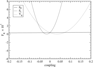
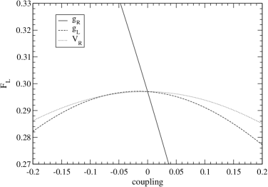
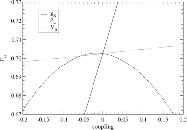
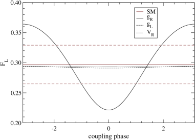
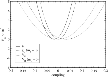
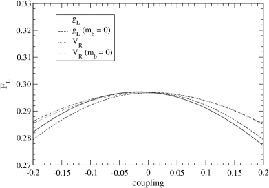
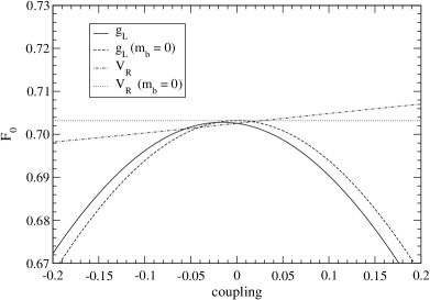
In the presence of anomalous couplings, the helicity fractions Fisubscript𝐹𝑖F_{i} are modified with respect to their SM values quoted above. Their variation is plotted in Fig.Β 2, considering that only one coupling is different from zero at a time and restricting ourselves to the CP-conserving case of real VRsubscript𝑉𝑅V_{R}, gRsubscript𝑔𝑅g_{R} and gLsubscript𝑔𝐿g_{L}. We observe that FLsubscript𝐹𝐿F_{L} and F0subscript𝐹0F_{0} are much more sensitive to gRsubscript𝑔𝑅g_{R} than to gLsubscript𝑔𝐿g_{L} and VRsubscript𝑉𝑅V_{R}. This is due to the interference term VL​gRβˆ—subscript𝑉𝐿superscriptsubscript𝑔𝑅V_{L}g_{R}^{*} , which is not suppressed by the bottom quark mass as for the gLsubscript𝑔𝐿g_{L} and VRsubscript𝑉𝑅V_{R} couplings. This linear term dominates over the quadratic one and makes the helicity fractions (and related quantities) very sensitive to gRsubscript𝑔𝑅g_{R}. We also remark that the phases of anomalous couplings influence the helicity fractions through the interference terms which depend on the real part of VRsubscript𝑉𝑅V_{R}, gLsubscript𝑔𝐿g_{L} and gRsubscript𝑔𝑅g_{R} (we have taken VLsubscript𝑉𝐿V_{L} real, and normalised to unity). Thus, the effect of complex phases is specially relevant for gRsubscript𝑔𝑅g_{R}, where the interference term dominates. In any case, the maximum and minimum deviations on the helicity fractions are found for real, positive and negative (not necessarily in this order) values of VRsubscript𝑉𝑅V_{R}, gRsubscript𝑔𝑅g_{R} and gLsubscript𝑔𝐿g_{L}. The possibility of complex couplings is examined with more detail in sectionΒ 6.

Refer to caption Refer to caption
Refer to caption
Figure 2: Dependence of the helicity fractions Fi=Ξ“i/Ξ“subscript𝐹𝑖subscriptΓ𝑖ΓF_{i}=\Gamma_{i}/\Gamma on the anomalous couplings in Eq.Β (1), in the CP-conserving case.

The helicity fractions can be experimentally extracted from a fit to the cosβ‘ΞΈβ„“βˆ—superscriptsubscriptπœƒβ„“\cos\theta_{\ell}^{*} distribution using Eq.Β (5). In order to estimate the limits on anomalous couplings that can be set from their measurement, we assume that the central values obtained correspond to the SM prediction, and take their errors from Refs.Β [19, 15, 16], giving F0≃0.703Β±0.016similar-to-or-equalssubscript𝐹0plus-or-minus0.7030.016F_{0}\simeq 0.703\pm 0.016, FR≃3.6Γ—10βˆ’4Β±0.0045similar-to-or-equalssubscript𝐹𝑅plus-or-minus3.6superscript1040.0045F_{R}\simeq 3.6\times 10^{-4}\pm 0.0045, FL≃0.297Β±0.016similar-to-or-equalssubscript𝐹𝐿plus-or-minus0.2970.016F_{L}\simeq 0.297\pm 0.016. For these values, it is found that F0subscript𝐹0F_{0} and FLsubscript𝐹𝐿F_{L} have a similar sensitivity to gRsubscript𝑔𝑅g_{R}, while the dependence of FRsubscript𝐹𝑅F_{R} on this coupling is smaller. On the other hand, the measurement of FRsubscript𝐹𝑅F_{R} sets the strongest constraint on VRsubscript𝑉𝑅V_{R} and gLsubscript𝑔𝐿g_{L}. The resulting bounds are summarised in the first column of TableΒ 1. These and the rest of limits throughout this paper have been obtained with a Monte Carlo method, as described in appendix B.

Fisubscript𝐹𝑖F_{i} ρisubscriptπœŒπ‘–\rho_{i}
VRsubscript𝑉𝑅V_{R} [βˆ’0.062,0.13]0.0620.13[-0.062,0.13] [βˆ’0.029,0.099]0.0290.099[-0.029,0.099]
gLsubscript𝑔𝐿g_{L} [βˆ’0.060,0.028]0.0600.028[-0.060,0.028] [βˆ’0.046,0.013]0.0460.013[-0.046,0.013]
gRsubscript𝑔𝑅g_{R} [βˆ’0.023,0.021]0.0230.021[-0.023,0.021] [βˆ’0.025,0.026]0.0250.026[-0.025,0.026]
Table 1: 1​σ1𝜎1\sigma bounds of anomalous couplings obtained from the measurement of helicity fractions Fisubscript𝐹𝑖F_{i} and ratios ρisubscriptπœŒπ‘–\rho_{i}.

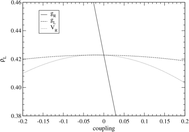
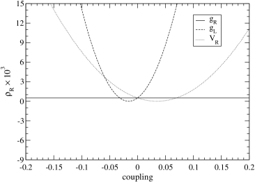
The sensitivity achieved for non-standard couplings may be greater if we consider instead the helicity ratios ρR,L≑ΓR,L/Ξ“0=FR,L/F0subscriptπœŒπ‘…πΏsubscriptΓ𝑅𝐿subscriptΞ“0subscript𝐹𝑅𝐿subscript𝐹0\rho_{R,L}\equiv\Gamma_{R,L}/\Gamma_{0}=F_{R,L}/F_{0}, shown in Fig.Β 3.222We note that, for a better comparison among them and with other observables, the scale of the y𝑦y axis in each plot is chosen so that the range approximately corresponds to two standard deviations (with the expected LHC precision) around the theoretical SM value. These ratios can be directly measured with a fit to the cosβ‘ΞΈβ„“βˆ—superscriptsubscriptπœƒβ„“\cos\theta_{\ell}^{*} distribution as well. From the expected precision in their determination in Ref.Β [15, 16], and assuming that the central values correspond to the SM prediction, we have ρR≃0.0005Β±0.0026similar-to-or-equalssubscriptπœŒπ‘…plus-or-minus0.00050.0026\rho_{R}\simeq 0.0005\pm 0.0026, ρL≃0.423Β±0.036similar-to-or-equalssubscript𝜌𝐿plus-or-minus0.4230.036\rho_{L}\simeq 0.423\pm 0.036. From these values, the limits given in the second column of TableΒ 1 can be obtained, with an important improvement for VRsubscript𝑉𝑅V_{R} and gLsubscript𝑔𝐿g_{L}. As it has been remarked in the introduction, the reason for the improvement is that systematic errors, which dominate the precision of the measurements (see Refs.Β [15, 16] for details), are much smaller for helicity ratios than for helicity fractions.
Refer to caption Refer to caption
Figure 3: Dependence of the helicity ratios ρR,L=Ξ“R,L/Ξ“0subscriptπœŒπ‘…πΏsubscriptΓ𝑅𝐿subscriptΞ“0\rho_{R,L}=\Gamma_{R,L}/\Gamma_{0} on the anomalous couplings in Eq.Β (1), in the CP-conserving case.

To conclude this section, we would like to stress the importance of keeping the bottom quark mass in the calculations. Within the SM the mbsubscriptπ‘šπ‘m_{b} correction to the helicity fractions is small, of order xb2=7.5Γ—10βˆ’4superscriptsubscriptπ‘₯𝑏27.5superscript104x_{b}^{2}=7.5\times 10^{-4}, as it can be seen in Eqs.Β (2). However, as it can also be observed, the interference terms involving gLsubscript𝑔𝐿g_{L} or VRsubscript𝑉𝑅V_{R} couplings with VLsubscript𝑉𝐿V_{L} are proportional to xb=0.027subscriptπ‘₯𝑏0.027x_{b}=0.027, and are of similar magnitude as the quadratic terms. The effect of including mbsubscriptπ‘šπ‘m_{b} in the computations is illustrated with more detail in appendix A. Nevertheless, we note here that if mbsubscriptπ‘šπ‘m_{b} is neglected the resulting confidence intervals on VRsubscript𝑉𝑅V_{R}, gLsubscript𝑔𝐿g_{L} are symmetric. The asymmetry between positive and negative couplings seen in TableΒ 1 reflects the importance of the mbsubscriptπ‘šπ‘m_{b} correction. It should also be noted that the mbsubscriptπ‘šπ‘m_{b} dependence of the limits leads to a small systematic uncertainty, due to the uncertainty in mbsubscriptπ‘šπ‘m_{b}. This is examined in detail in appendix A.

3 Angular asymmetries

A simple and efficient method to extract information about the W​t​bπ‘Šπ‘‘π‘Wtb vertex is through angular asymmetries involving the angle ΞΈβ„“βˆ—superscriptsubscriptπœƒβ„“\theta_{\ell}^{*} between the charged lepton momentum (in the Wπ‘ŠW boson rest frame) and the W+superscriptπ‘ŠW^{+} boson momentum (in the top quark rest frame). Alternatively, one may consider the angle θℓ​bsubscriptπœƒβ„“π‘\theta_{\ell b} between the charged lepton and b𝑏b quark momenta in the Wπ‘ŠW rest frame. Both approaches are equivalent since these two angles are related by ΞΈβ„“βˆ—+θℓ​b=Ο€superscriptsubscriptπœƒβ„“subscriptπœƒβ„“π‘πœ‹\theta_{\ell}^{*}+\theta_{\ell b}=\pi. (The determination of θℓ​bsubscriptπœƒβ„“π‘\theta_{\ell b}, however, is simpler, because both momenta are measured in the same reference frame without any ambiguity in the boosts.) For any fixed z𝑧z in the interval [βˆ’1,1]11[-1,1], one can define an asymmetry

Az=N​(cosβ‘ΞΈβ„“βˆ—>z)βˆ’N​(cosβ‘ΞΈβ„“βˆ—<z)N​(cosβ‘ΞΈβ„“βˆ—>z)+N​(cosβ‘ΞΈβ„“βˆ—<z).subscript𝐴𝑧𝑁superscriptsubscriptπœƒβ„“π‘§π‘superscriptsubscriptπœƒβ„“π‘§π‘superscriptsubscriptπœƒβ„“π‘§π‘superscriptsubscriptπœƒβ„“π‘§A_{z}=\frac{N(\cos\theta_{\ell}^{*}>z)-N(\cos\theta_{\ell}^{*}<z)}{N(\cos\theta_{\ell}^{*}>z)+N(\cos\theta_{\ell}^{*}<z)}\,. (7)

The most obvious choice is z=0𝑧0z=0, giving the forward-backward (FB) asymmetry AFBsubscript𝐴FBA_{\mathrm{FB}} [20, 9].333Notice the difference in sign with respect to the definitions in Refs.Β [20, 9], where θℓ​bsubscriptπœƒβ„“π‘\theta_{\ell b} is used. It is analogous to the FB asymmetries at LEP, which together with the ratios Rbsubscript𝑅𝑏R_{b}, Rcsubscript𝑅𝑐R_{c} allow us to extract the couplings of the c𝑐c and b𝑏b quarks to the Z𝑍Z boson. The FB asymmetry is related to the Wπ‘ŠW helicity fractions by

AFB=34​[FRβˆ’FL].subscript𝐴FB34delimited-[]subscript𝐹𝑅subscript𝐹𝐿A_{\mathrm{FB}}=\frac{3}{4}[F_{R}-F_{L}]\,. (8)

The measurement of this asymmetry alone is not enough to fully reconstruct the cosβ‘ΞΈβ„“βˆ—superscriptsubscriptπœƒβ„“\cos\theta_{\ell}^{*} distribution. One can then think about other asymmetries for different values of z𝑧z. The determination of Fisubscript𝐹𝑖F_{i} is easier if we construct asymmetries involving only FRsubscript𝐹𝑅F_{R} and F0subscript𝐹0F_{0}, or FLsubscript𝐹𝐿F_{L} and F0subscript𝐹0F_{0}. This is achieved choosing z=βˆ“(22/3βˆ’1)𝑧minus-or-plussuperscript2231z=\mp(2^{2/3}-1). Defining for convenience Ξ²=21/3βˆ’1𝛽superscript2131\beta=2^{1/3}-1, we have

z=βˆ’(22/3βˆ’1)𝑧superscript2231\displaystyle z=-(2^{2/3}-1) β†’β†’\displaystyle\rightarrow At=A+=3​β​[F0+(1+Ξ²)​FR],subscript𝐴𝑑subscript𝐴3𝛽delimited-[]subscript𝐹01𝛽subscript𝐹𝑅\displaystyle A_{t}=A_{+}=3\beta[F_{0}+(1+\beta)F_{R}]\,,
z=(22/3βˆ’1)𝑧superscript2231\displaystyle z=(2^{2/3}-1) β†’β†’\displaystyle\rightarrow At=Aβˆ’=βˆ’3​β​[F0+(1+Ξ²)​FL].subscript𝐴𝑑subscript𝐴3𝛽delimited-[]subscript𝐹01𝛽subscript𝐹𝐿\displaystyle A_{t}=A_{-}=-3\beta[F_{0}+(1+\beta)F_{L}]\,. (9)

From both asymmetries and using FR+FL+F0=1subscript𝐹𝑅subscript𝐹𝐿subscript𝐹01F_{R}+F_{L}+F_{0}=1, we obtain

FRsubscript𝐹𝑅\displaystyle F_{R} =\displaystyle= 11βˆ’Ξ²+Aβˆ’βˆ’Ξ²β€‹A+3​β​(1βˆ’Ξ²2),11𝛽subscript𝐴𝛽subscript𝐴3𝛽1superscript𝛽2\displaystyle\frac{1}{1-\beta}+\frac{A_{-}-\beta A_{+}}{3\beta(1-\beta^{2})}\,,
FLsubscript𝐹𝐿\displaystyle F_{L} =\displaystyle= 11βˆ’Ξ²βˆ’A+βˆ’Ξ²β€‹Aβˆ’3​β​(1βˆ’Ξ²2),11𝛽subscript𝐴𝛽subscript𝐴3𝛽1superscript𝛽2\displaystyle\frac{1}{1-\beta}-\frac{A_{+}-\beta A_{-}}{3\beta(1-\beta^{2})}\,,
F0subscript𝐹0\displaystyle F_{0} =\displaystyle= βˆ’1+Ξ²1βˆ’Ξ²+A+βˆ’Aβˆ’3​β​(1βˆ’Ξ²).1𝛽1𝛽subscript𝐴subscript𝐴3𝛽1𝛽\displaystyle-\frac{1+\beta}{1-\beta}+\frac{A_{+}-A_{-}}{3\beta(1-\beta)}\,. (10)
Refer to caption Refer to caption
Refer to caption
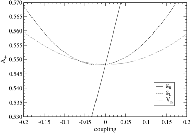
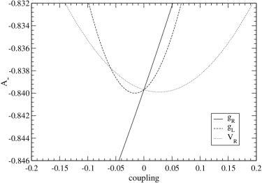
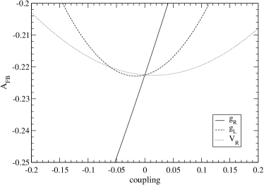
Figure 4: Dependence of the asymmetries A+subscript𝐴A_{+}, Aβˆ’subscript𝐴A_{-} and AFBsubscript𝐴FBA_{\mathrm{FB}} on the couplings gLsubscript𝑔𝐿g_{L}, gLsubscript𝑔𝐿g_{L} and VRsubscript𝑉𝑅V_{R}, for the CP-conserving case.

The three asymmetries AFBsubscript𝐴FBA_{\mathrm{FB}}, A+subscript𝐴A_{+}, Aβˆ’subscript𝐴A_{-} are quite sensitive to anomalous W​t​bπ‘Šπ‘‘π‘Wtb interactions. Their SM values are AFB=βˆ’0.2225subscript𝐴FB0.2225A_{\mathrm{FB}}=-0.2225, A+=0.5482subscript𝐴0.5482A_{+}=0.5482, Aβˆ’=βˆ’0.8397subscript𝐴0.8397A_{-}=-0.8397, and their dependence on the non-standard couplings is shown in Fig.Β 4. Taking the expected precision in their measurement from Refs.Β [15, 16] and assuming as central values the SM predictions, we obtain AFBβ‰ƒβˆ’0.223Β±0.013similar-to-or-equalssubscript𝐴FBplus-or-minus0.2230.013A_{\mathrm{FB}}\simeq-0.223\pm 0.013, A+≃0.548Β±0.010similar-to-or-equalssubscript𝐴plus-or-minus0.5480.010A_{+}\simeq 0.548\pm 0.010, Aβˆ’β‰ƒβˆ’0.8397Β±0.0033similar-to-or-equalssubscript𝐴plus-or-minus0.83970.0033A_{-}\simeq-0.8397\pm 0.0033. Using e.g. the latter two, the helicity fractions can be determined as

FRsubscript𝐹𝑅\displaystyle F_{R} =\displaystyle= 0.0017Β±0.0071,plus-or-minus0.00170.0071\displaystyle 0.0017\pm 0.0071\,,
FLsubscript𝐹𝐿\displaystyle F_{L} =\displaystyle= 0.2981±0.0167,plus-or-minus0.29810.0167\displaystyle 0.2981\pm 0.0167\,,
F0subscript𝐹0\displaystyle F_{0} =\displaystyle= 0.7002±0.0184.plus-or-minus0.70020.0184\displaystyle 0.7002\pm 0.0184\,. (11)

The errors quoted take into account the correlation between the two measurements, which is determined writing the asymmetries in terms of the numbers of events in three bins: [βˆ’1,βˆ’(22/3βˆ’1)]1superscript2231[-1,-(2^{2/3}-1)], [βˆ’(22/3βˆ’1),(22/3βˆ’1)]superscript2231superscript2231[-(2^{2/3}-1),(2^{2/3}-1)] and [(22/3βˆ’1),1]superscript22311[(2^{2/3}-1),1]. We omit these details for brevity. The values extracted in this way are less precise than if obtained from a direct fit, but the method employed is much simpler too. The eventual limits which would be extracted from asymmetry measurements are collected in TableΒ 2. A+subscript𝐴A_{+} exhibits the strongest dependence on gRsubscript𝑔𝑅g_{R} and, if measured as precisely as it is expected, it would set the best limits on this coupling. On the other hand, Aβˆ’subscript𝐴A_{-} is the most sensitive to VRsubscript𝑉𝑅V_{R} and gLsubscript𝑔𝐿g_{L} and sets the strongest bounds on them. The limits obtained from asymmetry measurements are competitive with those obtained from a direct fit to the cosβ‘ΞΈβ„“βˆ—superscriptsubscriptπœƒβ„“\cos\theta_{\ell}^{*} distribution.

A+subscript𝐴A_{+} Aβˆ’subscript𝐴A_{-} AFBsubscript𝐴FBA_{\mathrm{FB}}
VRsubscript𝑉𝑅V_{R} [βˆ’0.15,0.15]0.150.15[-0.15,0.15] [βˆ’0.056,0.11]0.0560.11[-0.056,0.11] [βˆ’0.12,0.15]0.120.15[-0.12,0.15]
gLsubscript𝑔𝐿g_{L} [βˆ’0.12,0.082]0.120.082[-0.12,0.082] [βˆ’0.057,0.026]0.0570.026[-0.057,0.026] [βˆ’0.092,0.062]0.0920.062[-0.092,0.062]
gRsubscript𝑔𝑅g_{R} [βˆ’0.019,0.018]0.0190.018[-0.019,0.018] [βˆ’0.024,0.022]0.0240.022[-0.024,0.022] [βˆ’0.027,0.025]0.0270.025[-0.027,0.025]
Table 2: 1​σ1𝜎1\sigma bounds on anomalous couplings obtained from the measurement of angular asymmetries.

4 Energy distributions

The charged lepton energy in the Wπ‘ŠW rest frame is fixed by the kinematics of the two-body decay Wβ†’β„“β€‹Ξ½β†’π‘Šβ„“πœˆW\to\ell\nu. Its energy in the top quark rest frame, denoted from now on by Eβ„“subscript𝐸ℓE_{\ell}, is related to the former by a Lorentz boost, and it is given by

Eβ„“=12​(EW+|qβ†’|​cosβ‘ΞΈβ„“βˆ—),subscript𝐸ℓ12subscriptπΈπ‘Šβ†’π‘žsuperscriptsubscriptπœƒβ„“E_{\ell}=\frac{1}{2}(E_{W}+|\vec{q}\,|\cos\theta_{\ell}^{*})\,, (12)

with |qβ†’|β†’π‘ž|\vec{q}\,|, given in Eq.Β (3), the Wπ‘ŠW boson momentum in the top rest frame and EWsubscriptπΈπ‘ŠE_{W} its energy. Therefore, the angular distribution of the charged lepton in Wπ‘ŠW rest frame determines its energy in the top rest frame. The maximum and minimum energies are Emax=(EW+|qβ†’|)/2subscript𝐸maxsubscriptπΈπ‘Šβ†’π‘ž2E_{\text{max}}=(E_{W}+|\vec{q}\,|)/2, Emin=(EWβˆ’|qβ†’|)/2subscript𝐸minsubscriptπΈπ‘Šβ†’π‘ž2E_{\text{min}}=(E_{W}-|\vec{q}\,|)/2. The energy distribution is obtained from Eqs.Β (5) and (12),

1Γ​d​Γd​Eβ„“1Γ𝑑Γ𝑑subscript𝐸ℓ\displaystyle\frac{1}{\Gamma}\frac{d\Gamma}{dE_{\ell}} =\displaystyle= 1(Emaxβˆ’Emin)3[3(Eβ„“βˆ’Emin)2FR+3(Emaxβˆ’Eβ„“)2FL\displaystyle\frac{1}{(E_{\text{max}}-E_{\text{min}})^{3}}\left[3(E_{\ell}-E_{\text{min}})^{2}\,F_{R}+3(E_{\text{max}}-E_{\ell})^{2}\,F_{L}\right. (13)
+6(Emaxβˆ’Eβ„“)(Eβ„“βˆ’Emin)F0].\displaystyle\left.+6(E_{\text{max}}-E_{\ell})(E_{\ell}-E_{\text{min}})\,F_{0}\right]\,.

The description of the top decay in terms of cosβ‘ΞΈβ„“βˆ—superscriptsubscriptπœƒβ„“\cos\theta_{\ell}^{*} or Eβ„“subscript𝐸ℓE_{\ell} seems then equivalent, up to a change of variables. Any asymmetry built using cosβ‘ΞΈβ„“βˆ—superscriptsubscriptπœƒβ„“\cos\theta_{\ell}^{*}, defined around a fixed value z𝑧z, can be translated into an equivalent asymmetry involving Eβ„“subscript𝐸ℓE_{\ell}, defined around a fixed energy Ez=(EW+|qβ†’|​z)/2subscript𝐸𝑧subscriptπΈπ‘Šβ†’π‘žπ‘§2E_{z}=(E_{W}+|\vec{q}\,|\,z)/2, namely

Az=N​(Eβ„“>Ez)βˆ’N​(Eβ„“<Ez)N​(Eβ„“>Ez)+N​(Eβ„“<Ez).subscript𝐴𝑧𝑁subscript𝐸ℓsubscript𝐸𝑧𝑁subscript𝐸ℓsubscript𝐸𝑧𝑁subscript𝐸ℓsubscript𝐸𝑧𝑁subscript𝐸ℓsubscript𝐸𝑧A_{z}=\frac{N(E_{\ell}>E_{z})-N(E_{\ell}<E_{z})}{N(E_{\ell}>E_{z})+N(E_{\ell}<E_{z})}\,. (14)

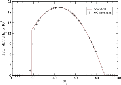
However, in contrast to what was demonstrated in sectionΒ 2 for the angular distributions, finite width corrections have a non-negligible influence on Eβ„“subscript𝐸ℓE_{\ell}. This can be seen in Fig.Β 5, where we plot the energy distribution calculated analytically for t𝑑t and Wπ‘ŠW on shell and from a Monte Carlo calculation including finite width effects. The values of the asymmetries A+subscript𝐴A_{+}, Aβˆ’subscript𝐴A_{-} and AFBsubscript𝐴FBA_{\mathrm{FB}}, calculated analytically and numerically (the latter for the cosβ‘ΞΈβ„“βˆ—superscriptsubscriptπœƒβ„“\cos\theta_{\ell}^{*} and Eβ„“subscript𝐸ℓE_{\ell} distributions) are shown in TableΒ 3. One can notice the larger influence of finite width corrections for energy asymmetries.
Refer to caption
Figure 5: Differential distribution in Eq.Β (13) within the SM, calculated analytically and with a Monte Carlo simulation.
Analytical Angular Energy
A+subscript𝐴A_{+} 0.5482 0.5492 0.5529
Aβˆ’subscript𝐴A_{-} -0.8397 -0.8393 -0.8339
AFBsubscript𝐴FBA_{\mathrm{FB}} -0.2225 -0.2212 -0.2166
Table 3: Values of the asymmetries A+subscript𝐴A_{+}, Aβˆ’subscript𝐴A_{-}, AFBsubscript𝐴FBA_{\mathrm{FB}} obtained from the analytical expression (first column) and from the Monte Carlo simulation, the latter from the measurement of the distributions of cosβ‘ΞΈβ„“βˆ—superscriptsubscriptπœƒβ„“\cos\theta_{\ell}^{*} (second column) and Elsubscript𝐸𝑙E_{l} (third column).

The expected precision in energy asymmetries is worse than for the angular ones (given in the previous section) as it might be expected: AFBβ‰ƒβˆ’0.223Β±0.024similar-to-or-equalssubscript𝐴FBplus-or-minus0.2230.024A_{\mathrm{FB}}\simeq-0.223\pm 0.024, A+≃0.548Β±0.013similar-to-or-equalssubscript𝐴plus-or-minus0.5480.013A_{+}\simeq 0.548\pm 0.013, Aβˆ’β‰ƒβˆ’0.840Β±0.016similar-to-or-equalssubscript𝐴plus-or-minus0.8400.016A_{-}\simeq-0.840\pm 0.016. Therefore, in principle their study does not seem to bring any improvement from the experimental side.

5 Spin asymmetries

Additional angular asymmetries can be built involving the top spin. Top quarks are produced unpolarised at the tree level in QCD interactions, and with a very small O​(10βˆ’2)𝑂superscript102O(10^{-2}) transverse polarisation at one loop. However, the t𝑑t and t¯¯𝑑\bar{t} spins are strongly correlated, what allows the construction of angular asymmetries at the percent level. The top (anti)quark spins are not directly observable, but influence the angular distribution of their decay products. For the decay tβ†’W+​bβ†’β„“+​ν​b,q​q¯′​bformulae-sequence→𝑑superscriptπ‘Šπ‘β†’superscriptβ„“πœˆπ‘π‘žsuperscriptΒ―π‘žβ€²π‘t\to W^{+}b\to\ell^{+}\nu b,q\bar{q}^{\prime}b, the angular distributions of X=β„“+,Ξ½,q,qΒ―β€²,W+,b𝑋superscriptβ„“πœˆπ‘žsuperscriptΒ―π‘žβ€²superscriptπ‘Šπ‘X=\ell^{+},\nu,q,\bar{q}^{\prime},W^{+},b (which are called β€œspin analysers”) in the top quark rest frame are given by

1Γ​d​Γd​cos⁑θX=12​(1+Ξ±X​cos⁑θX)1Γ𝑑Γ𝑑subscriptπœƒπ‘‹121subscript𝛼𝑋subscriptπœƒπ‘‹\frac{1}{\Gamma}\frac{d\Gamma}{d\cos\theta_{X}}=\frac{1}{2}(1+\alpha_{X}\cos\theta_{X}) (15)

with ΞΈXsubscriptπœƒπ‘‹\theta_{X} the angle between the three-momentum of X𝑋X (in the t𝑑t rest frame) and the top spin direction. The constants Ξ±Xsubscript𝛼𝑋\alpha_{X} are called β€œspin analysing power” of X𝑋X and can range between βˆ’11-1 and 111. In the SM, Ξ±β„“+=Ξ±qΒ―β€²=1subscript𝛼superscriptβ„“subscript𝛼superscriptΒ―π‘žβ€²1\alpha_{\ell^{+}}=\alpha_{\bar{q}^{\prime}}=1, Ξ±Ξ½=Ξ±q=βˆ’0.32subscriptπ›Όπœˆsubscriptπ›Όπ‘ž0.32\alpha_{\nu}=\alpha_{q}=-0.32, Ξ±W+=βˆ’Ξ±b=0.41subscript𝛼superscriptπ‘Šsubscript𝛼𝑏0.41\alpha_{W^{+}}=-\alpha_{b}=0.41 at the tree level [21] (qπ‘žq and qβ€²superscriptπ‘žβ€²q^{\prime} are the up- and down-type quarks, respectively, resulting from the Wπ‘ŠW decay). For the decay of a top antiquark the distributions are the same, with Ξ±XΒ―=βˆ’Ξ±Xsubscript𝛼¯𝑋subscript𝛼𝑋\alpha_{\bar{X}}=-\alpha_{X} as long as CP is conserved in the decay. One-loop corrections modify these values to Ξ±β„“+=0.998subscript𝛼superscriptβ„“0.998\alpha_{\ell^{+}}=0.998, Ξ±qΒ―β€²=0.93subscript𝛼superscriptΒ―π‘žβ€²0.93\alpha_{\bar{q}^{\prime}}=0.93, Ξ±Ξ½=βˆ’0.33subscriptπ›Όπœˆ0.33\alpha_{\nu}=-0.33, Ξ±q=βˆ’0.31subscriptπ›Όπ‘ž0.31\alpha_{q}=-0.31, Ξ±W+=βˆ’Ξ±b=0.39subscript𝛼superscriptπ‘Šsubscript𝛼𝑏0.39\alpha_{W^{+}}=-\alpha_{b}=0.39 [22, 23]. We point out that in the presence of non-vanishing VRsubscript𝑉𝑅V_{R}, gLsubscript𝑔𝐿g_{L} or gRsubscript𝑔𝑅g_{R} couplings the numerical values of the constants Ξ±Xsubscript𝛼𝑋\alpha_{X} are modified, but the functional form of Eq.Β (15) is maintained. We have explicitly calculated them for a general CP-conserving W​t​bπ‘Šπ‘‘π‘Wtb vertex as written in Eq.Β (1) within the narrow width approximation. They can be written as Ξ±X=aX/a0subscript𝛼𝑋subscriptπ‘Žπ‘‹subscriptπ‘Ž0\alpha_{X}=a_{X}/a_{0}, with

a0subscriptπ‘Ž0\displaystyle a_{0} =[VL2+VR2]​(1+xW2βˆ’2​xb2βˆ’2​xW4+xW2​xb2+xb4)βˆ’12​xW2​xb​VL​VRabsentdelimited-[]superscriptsubscript𝑉𝐿2superscriptsubscript𝑉𝑅21superscriptsubscriptπ‘₯π‘Š22superscriptsubscriptπ‘₯𝑏22superscriptsubscriptπ‘₯π‘Š4superscriptsubscriptπ‘₯π‘Š2superscriptsubscriptπ‘₯𝑏2superscriptsubscriptπ‘₯𝑏412superscriptsubscriptπ‘₯π‘Š2subscriptπ‘₯𝑏subscript𝑉𝐿subscript𝑉𝑅\displaystyle=\left[V_{L}^{2}+V_{R}^{2}\right]\left(1+x_{W}^{2}-2x_{b}^{2}-2x_{W}^{4}+x_{W}^{2}x_{b}^{2}+x_{b}^{4}\right)-12x_{W}^{2}x_{b}\,V_{L}V_{R}
+2​[gL2+gR2]​(1βˆ’xW22βˆ’2​xb2βˆ’xW42βˆ’xW2​xb22+xb4)2delimited-[]superscriptsubscript𝑔𝐿2superscriptsubscript𝑔𝑅21superscriptsubscriptπ‘₯π‘Š222superscriptsubscriptπ‘₯𝑏2superscriptsubscriptπ‘₯π‘Š42superscriptsubscriptπ‘₯π‘Š2superscriptsubscriptπ‘₯𝑏22superscriptsubscriptπ‘₯𝑏4\displaystyle+2\left[g_{L}^{2}+g_{R}^{2}\right]\left(1-\frac{x_{W}^{2}}{2}-2x_{b}^{2}-\frac{x_{W}^{4}}{2}-\frac{x_{W}^{2}x_{b}^{2}}{2}+x_{b}^{4}\right)
βˆ’12​xW2​xb​gL​gRβˆ’6​xW​[VL​gR+VR​gL]​(1βˆ’xW2βˆ’xb2)12superscriptsubscriptπ‘₯π‘Š2subscriptπ‘₯𝑏subscript𝑔𝐿subscript𝑔𝑅6subscriptπ‘₯π‘Šdelimited-[]subscript𝑉𝐿subscript𝑔𝑅subscript𝑉𝑅subscript𝑔𝐿1superscriptsubscriptπ‘₯π‘Š2superscriptsubscriptπ‘₯𝑏2\displaystyle-12x_{W}^{2}x_{b}\,g_{L}g_{R}-6x_{W}\left[V_{L}g_{R}+V_{R}g_{L}\right]\left(1-x_{W}^{2}-x_{b}^{2}\right)
+6​xW​xb​[VL​gL+VR​gR]​(1+xW2βˆ’xb2),6subscriptπ‘₯π‘Šsubscriptπ‘₯𝑏delimited-[]subscript𝑉𝐿subscript𝑔𝐿subscript𝑉𝑅subscript𝑔𝑅1superscriptsubscriptπ‘₯π‘Š2superscriptsubscriptπ‘₯𝑏2\displaystyle+6x_{W}x_{b}\,\left[V_{L}g_{L}+V_{R}g_{R}\right]\left(1+x_{W}^{2}-x_{b}^{2}\right)\,,
aβ„“+,qΒ―β€²subscriptπ‘Žsuperscriptβ„“superscriptΒ―π‘žβ€²\displaystyle a_{\ell^{+},\bar{q}^{\prime}} =[VL2βˆ’VR2]​(1+xW2βˆ’2​xb2βˆ’2​xW4+xW2​xb2+xb4)βˆ’12​xW2​xb​VL​VRabsentdelimited-[]superscriptsubscript𝑉𝐿2superscriptsubscript𝑉𝑅21superscriptsubscriptπ‘₯π‘Š22superscriptsubscriptπ‘₯𝑏22superscriptsubscriptπ‘₯π‘Š4superscriptsubscriptπ‘₯π‘Š2superscriptsubscriptπ‘₯𝑏2superscriptsubscriptπ‘₯𝑏412superscriptsubscriptπ‘₯π‘Š2subscriptπ‘₯𝑏subscript𝑉𝐿subscript𝑉𝑅\displaystyle=\left[V_{L}^{2}-V_{R}^{2}\right]\left(1+x_{W}^{2}-2x_{b}^{2}-2x_{W}^{4}+x_{W}^{2}x_{b}^{2}+x_{b}^{4}\right)-12x_{W}^{2}x_{b}\,V_{L}V_{R}
+2​[gL2βˆ’gR2]​(1βˆ’xW22βˆ’2​xb2βˆ’xW42βˆ’xW2​xb22+xb4)2delimited-[]superscriptsubscript𝑔𝐿2superscriptsubscript𝑔𝑅21superscriptsubscriptπ‘₯π‘Š222superscriptsubscriptπ‘₯𝑏2superscriptsubscriptπ‘₯π‘Š42superscriptsubscriptπ‘₯π‘Š2superscriptsubscriptπ‘₯𝑏22superscriptsubscriptπ‘₯𝑏4\displaystyle+2\left[g_{L}^{2}-g_{R}^{2}\right]\left(1-\frac{x_{W}^{2}}{2}-2x_{b}^{2}-\frac{x_{W}^{4}}{2}-\frac{x_{W}^{2}x_{b}^{2}}{2}+x_{b}^{4}\right)
βˆ’12​xW2​xb​gL​gRβˆ’6​xW​[VL​gR+VR​gL]​(1βˆ’xW2βˆ’xb2)12superscriptsubscriptπ‘₯π‘Š2subscriptπ‘₯𝑏subscript𝑔𝐿subscript𝑔𝑅6subscriptπ‘₯π‘Šdelimited-[]subscript𝑉𝐿subscript𝑔𝑅subscript𝑉𝑅subscript𝑔𝐿1superscriptsubscriptπ‘₯π‘Š2superscriptsubscriptπ‘₯𝑏2\displaystyle-12x_{W}^{2}x_{b}\,g_{L}g_{R}-6x_{W}\left[V_{L}g_{R}+V_{R}g_{L}\right]\left(1-x_{W}^{2}-x_{b}^{2}\right)
+6​xW​xb​[VL​gLβˆ’VR​gR]​(1+xW2βˆ’xb2)+12​xW2​(VR2βˆ’gR2)6subscriptπ‘₯π‘Šsubscriptπ‘₯𝑏delimited-[]subscript𝑉𝐿subscript𝑔𝐿subscript𝑉𝑅subscript𝑔𝑅1superscriptsubscriptπ‘₯π‘Š2superscriptsubscriptπ‘₯𝑏212superscriptsubscriptπ‘₯π‘Š2superscriptsubscript𝑉𝑅2superscriptsubscript𝑔𝑅2\displaystyle+6x_{W}x_{b}\,\left[V_{L}g_{L}-V_{R}g_{R}\right]\left(1+x_{W}^{2}-x_{b}^{2}\right)+12x_{W}^{2}(V_{R}^{2}-g_{R}^{2})
+mt|qβ†’|​log⁑EW+|qβ†’|EWβˆ’|qβ†’|​[βˆ’6​xW4​VR2+6​xW2​gR2​(1βˆ’xb2)+12​xW3​xb​VR​gR],subscriptπ‘šπ‘‘β†’π‘žsubscriptπΈπ‘Šβ†’π‘žsubscriptπΈπ‘Šβ†’π‘ždelimited-[]6superscriptsubscriptπ‘₯π‘Š4superscriptsubscript𝑉𝑅26superscriptsubscriptπ‘₯π‘Š2superscriptsubscript𝑔𝑅21superscriptsubscriptπ‘₯𝑏212superscriptsubscriptπ‘₯π‘Š3subscriptπ‘₯𝑏subscript𝑉𝑅subscript𝑔𝑅\displaystyle+\frac{m_{t}}{|\vec{q}|}\log\frac{E_{W}+|\vec{q}|}{E_{W}-|\vec{q}|}\left[-6x_{W}^{4}V_{R}^{2}+6x_{W}^{2}g_{R}^{2}(1-x_{b}^{2})+12x_{W}^{3}x_{b}V_{R}g_{R}\right]\,,
aΞ½,qsubscriptπ‘Žπœˆπ‘ž\displaystyle a_{\nu,q} =[VL2βˆ’VR2]​(1+xW2βˆ’2​xb2βˆ’2​xW4+xW2​xb2+xb4)+12​xW2​xb​VL​VRabsentdelimited-[]superscriptsubscript𝑉𝐿2superscriptsubscript𝑉𝑅21superscriptsubscriptπ‘₯π‘Š22superscriptsubscriptπ‘₯𝑏22superscriptsubscriptπ‘₯π‘Š4superscriptsubscriptπ‘₯π‘Š2superscriptsubscriptπ‘₯𝑏2superscriptsubscriptπ‘₯𝑏412superscriptsubscriptπ‘₯π‘Š2subscriptπ‘₯𝑏subscript𝑉𝐿subscript𝑉𝑅\displaystyle=\left[V_{L}^{2}-V_{R}^{2}\right]\left(1+x_{W}^{2}-2x_{b}^{2}-2x_{W}^{4}+x_{W}^{2}x_{b}^{2}+x_{b}^{4}\right)+12x_{W}^{2}x_{b}\,V_{L}V_{R}
+2​[gL2βˆ’gR2]​(1βˆ’xW22βˆ’2​xb2βˆ’xW42βˆ’xW2​xb22+xb4)2delimited-[]superscriptsubscript𝑔𝐿2superscriptsubscript𝑔𝑅21superscriptsubscriptπ‘₯π‘Š222superscriptsubscriptπ‘₯𝑏2superscriptsubscriptπ‘₯π‘Š42superscriptsubscriptπ‘₯π‘Š2superscriptsubscriptπ‘₯𝑏22superscriptsubscriptπ‘₯𝑏4\displaystyle+2\left[g_{L}^{2}-g_{R}^{2}\right]\left(1-\frac{x_{W}^{2}}{2}-2x_{b}^{2}-\frac{x_{W}^{4}}{2}-\frac{x_{W}^{2}x_{b}^{2}}{2}+x_{b}^{4}\right)
+12​xW2​xb​gL​gR+6​xW​[VL​gR+VR​gL]​(1βˆ’xW2βˆ’xb2)12superscriptsubscriptπ‘₯π‘Š2subscriptπ‘₯𝑏subscript𝑔𝐿subscript𝑔𝑅6subscriptπ‘₯π‘Šdelimited-[]subscript𝑉𝐿subscript𝑔𝑅subscript𝑉𝑅subscript𝑔𝐿1superscriptsubscriptπ‘₯π‘Š2superscriptsubscriptπ‘₯𝑏2\displaystyle+12x_{W}^{2}x_{b}\,g_{L}g_{R}+6x_{W}\left[V_{L}g_{R}+V_{R}g_{L}\right]\left(1-x_{W}^{2}-x_{b}^{2}\right)
+6​xW​xb​[VL​gLβˆ’VR​gR]​(1+xW2βˆ’xb2)βˆ’12​xW2​(VL2βˆ’gL2)6subscriptπ‘₯π‘Šsubscriptπ‘₯𝑏delimited-[]subscript𝑉𝐿subscript𝑔𝐿subscript𝑉𝑅subscript𝑔𝑅1superscriptsubscriptπ‘₯π‘Š2superscriptsubscriptπ‘₯𝑏212superscriptsubscriptπ‘₯π‘Š2superscriptsubscript𝑉𝐿2superscriptsubscript𝑔𝐿2\displaystyle+6x_{W}x_{b}\,\left[V_{L}g_{L}-V_{R}g_{R}\right]\left(1+x_{W}^{2}-x_{b}^{2}\right)-12x_{W}^{2}(V_{L}^{2}-g_{L}^{2})
+mt|qβ†’|​log⁑EW+|qβ†’|EWβˆ’|qβ†’|​[6​xW4​VL2βˆ’6​xW2​gL2​(1βˆ’xb2)βˆ’12​xW3​xb​VL​gL],subscriptπ‘šπ‘‘β†’π‘žsubscriptπΈπ‘Šβ†’π‘žsubscriptπΈπ‘Šβ†’π‘ždelimited-[]6superscriptsubscriptπ‘₯π‘Š4superscriptsubscript𝑉𝐿26superscriptsubscriptπ‘₯π‘Š2superscriptsubscript𝑔𝐿21superscriptsubscriptπ‘₯𝑏212superscriptsubscriptπ‘₯π‘Š3subscriptπ‘₯𝑏subscript𝑉𝐿subscript𝑔𝐿\displaystyle+\frac{m_{t}}{|\vec{q}|}\log\frac{E_{W}+|\vec{q}|}{E_{W}-|\vec{q}|}\left[6x_{W}^{4}V_{L}^{2}-6x_{W}^{2}g_{L}^{2}(1-x_{b}^{2})-12x_{W}^{3}x_{b}V_{L}g_{L}\right]\,,
absubscriptπ‘Žπ‘\displaystyle a_{b} =βˆ’2|qβ†’|mt{[VL2βˆ’VR2](1βˆ’2xW2βˆ’xb2)+2[gL2βˆ’gR2](1βˆ’xW22+xb2)\displaystyle=-2\frac{|\vec{q}|}{m_{t}}\left\{\left[V_{L}^{2}-V_{R}^{2}\right]\left(1-2x_{W}^{2}-x_{b}^{2}\right)+2\left[g_{L}^{2}-g_{R}^{2}\right]\left(1-\frac{x_{W}^{2}}{2}+x_{b}^{2}\right)\right.
+2xW[VLgRβˆ’VRgL]+6xWxb[VLgLβˆ’VRgR]},\displaystyle\left.+2x_{W}\left[V_{L}g_{R}-V_{R}g_{L}\right]+6x_{W}x_{b}\left[V_{L}g_{L}-V_{R}g_{R}\right]\right\}\,, (16)

and aW=βˆ’absubscriptπ‘Žπ‘Šsubscriptπ‘Žπ‘a_{W}=-a_{b}. We have checked that our expressions are compatible with the first-order expansions in Refs.Β [24, 25]. Working in the helicity basis and neglecting small spin interference effects, so that the cross section factorises into production times decay factors, the double angular distribution of the decay products X𝑋X (from t𝑑t) and XΒ―β€²superscript¯𝑋′\bar{X}^{\prime} (from t¯¯𝑑\bar{t}) can be written as [26]

1σ​d​σd​cos⁑θX​d​cos⁑θXΒ―β€²=14​(1+C​αX​αX¯′​cos⁑θX​cos⁑θXΒ―β€²).1πœŽπ‘‘πœŽπ‘‘subscriptπœƒπ‘‹π‘‘subscriptπœƒsuperscript¯𝑋′141𝐢subscript𝛼𝑋subscript𝛼superscript¯𝑋′subscriptπœƒπ‘‹subscriptπœƒsuperscript¯𝑋′\frac{1}{\sigma}\frac{d\sigma}{d\cos\theta_{X}\,d\cos\theta_{\bar{X}^{\prime}}}=\frac{1}{4}(1+C\,\alpha_{X}\alpha_{\bar{X}^{\prime}}\cos\theta_{X}\cos\theta_{\bar{X}^{\prime}})\,. (17)

The angles ΞΈXsubscriptπœƒπ‘‹\theta_{X}, ΞΈXΒ―β€²subscriptπœƒsuperscript¯𝑋′\theta_{\bar{X}^{\prime}} are measured using as spin axis the parent top (anti)quark momentum in the t​t¯𝑑¯𝑑t\bar{t} CM system. The factor

C≑σ​(tR​tΒ―R)+σ​(tL​tΒ―L)βˆ’Οƒβ€‹(tR​tΒ―L)βˆ’Οƒβ€‹(tL​tΒ―R)σ​(tR​tΒ―R)+σ​(tL​tΒ―L)+σ​(tR​tΒ―L)+σ​(tL​tΒ―R)𝐢𝜎subscript𝑑𝑅subscriptΒ―π‘‘π‘…πœŽsubscript𝑑𝐿subscriptΒ―π‘‘πΏπœŽsubscript𝑑𝑅subscriptΒ―π‘‘πΏπœŽsubscript𝑑𝐿subscriptΒ―π‘‘π‘…πœŽsubscript𝑑𝑅subscriptΒ―π‘‘π‘…πœŽsubscript𝑑𝐿subscriptΒ―π‘‘πΏπœŽsubscript𝑑𝑅subscriptΒ―π‘‘πΏπœŽsubscript𝑑𝐿subscript¯𝑑𝑅C\equiv\frac{\sigma(t_{R}\bar{t}_{R})+\sigma(t_{L}\bar{t}_{L})-\sigma(t_{R}\bar{t}_{L})-\sigma(t_{L}\bar{t}_{R})}{\sigma(t_{R}\bar{t}_{R})+\sigma(t_{L}\bar{t}_{L})+\sigma(t_{R}\bar{t}_{L})+\sigma(t_{L}\bar{t}_{R})} (18)

is the relative number of like helicity minus opposite helicity t​t¯𝑑¯𝑑t\bar{t} pairs, and measures the spin correlation between the top quark and antiquark.444Other conventions in the literature (e.g. Refs.Β [27, 23]) denote by βˆ’C𝐢-C what in our case is the product C​αX​αX¯′𝐢subscript𝛼𝑋subscript𝛼superscript¯𝑋′C\,\alpha_{X}\alpha_{\bar{X}^{\prime}}. We prefer to keep the notation in Refs.Β [26, 1] and separate the contributions from the production (C𝐢C) and the decay (Ξ±Xsubscript𝛼𝑋\alpha_{X}, Ξ±XΒ―β€²subscript𝛼superscript¯𝑋′\alpha_{\bar{X}^{\prime}}) since the former is sensitive to new physics in the t​t¯𝑑¯𝑑t\bar{t} production process while the latter are sensitive to non-standard W​t​bπ‘Šπ‘‘π‘Wtb interactions. This decomposition is not possible if non-factorisable radiative corrections to the production and decay process are included. Anyway, these corrections are expected to be small. We note that due to P invariance of the QCD interactions, σ​(tR​tΒ―L)=σ​(tL​tΒ―R)𝜎subscript𝑑𝑅subscriptΒ―π‘‘πΏπœŽsubscript𝑑𝐿subscript¯𝑑𝑅\sigma(t_{R}\bar{t}_{L})=\sigma(t_{L}\bar{t}_{R}), and by CP conservation σ​(tR​tΒ―R)=σ​(tL​tΒ―L)𝜎subscript𝑑𝑅subscriptΒ―π‘‘π‘…πœŽsubscript𝑑𝐿subscript¯𝑑𝐿\sigma(t_{R}\bar{t}_{R})=\sigma(t_{L}\bar{t}_{L}). This is the reason why terms linear in cos⁑θXsubscriptπœƒπ‘‹\cos\theta_{X}, cos⁑θXΒ―β€²subscriptπœƒsuperscript¯𝑋′\cos\theta_{\bar{X}^{\prime}} are absent in Eq.Β (17). In other words, terms linear in the cosines are present only if the top quarks are produced with a net polarisation in the helicity basis, what does not happen in pure QCD production. The actual value of C𝐢C depends to some extent on the parton distribution functions (PDFs) used and the Q2superscript𝑄2Q^{2} scale at which they are evaluated. Using the CTEQ5L PDFs [28] and Q2=s^superscript𝑄2^𝑠Q^{2}=\hat{s} the partonic CM energy, we find C=0.310𝐢0.310C=0.310. At the one loop level, C=0.326Β±0.012𝐢plus-or-minus0.3260.012C=0.326\pm 0.012 [23].

Using the spin analysers X𝑋X, XΒ―β€²superscript¯𝑋′\bar{X}^{\prime} for the respective decays of t𝑑t, t¯¯𝑑\bar{t}, one can define the asymmetries

AX​X¯′≑N​(cos⁑θX​cos⁑θXΒ―β€²>0)βˆ’N​(cos⁑θX​cos⁑θXΒ―β€²<0)N​(cos⁑θX​cos⁑θXΒ―β€²>0)+N​(cos⁑θX​cos⁑θXΒ―β€²<0),subscript𝐴𝑋superscript¯𝑋′𝑁subscriptπœƒπ‘‹subscriptπœƒsuperscript¯𝑋′0𝑁subscriptπœƒπ‘‹subscriptπœƒsuperscript¯𝑋′0𝑁subscriptπœƒπ‘‹subscriptπœƒsuperscript¯𝑋′0𝑁subscriptπœƒπ‘‹subscriptπœƒsuperscript¯𝑋′0A_{X\bar{X}^{\prime}}\equiv\frac{N(\cos\theta_{X}\cos\theta_{\bar{X}^{\prime}}>0)-N(\cos\theta_{X}\cos\theta_{\bar{X}^{\prime}}<0)}{N(\cos\theta_{X}\cos\theta_{\bar{X}^{\prime}}>0)+N(\cos\theta_{X}\cos\theta_{\bar{X}^{\prime}}<0)}\,, (19)

whose theoretical value derived from Eq.Β (17) is

AX​XΒ―β€²=14​C​αX​αXΒ―β€².subscript𝐴𝑋superscript¯𝑋′14𝐢subscript𝛼𝑋subscript𝛼superscript¯𝑋′A_{X\bar{X}^{\prime}}=\frac{1}{4}C\alpha_{X}\alpha_{\bar{X}^{\prime}}\,. (20)

If CP is conserved in the decay, for charge conjugate decay channels we have Ξ±X′​αXΒ―=Ξ±X​αXΒ―β€²subscript𝛼superscript𝑋′subscript𝛼¯𝑋subscript𝛼𝑋subscript𝛼superscript¯𝑋′\alpha_{X^{\prime}}\alpha_{\bar{X}}=\alpha_{X}\alpha_{\bar{X}^{\prime}}, so the asymmetries AX′​XΒ―=AX​XΒ―β€²subscript𝐴superscript𝑋′¯𝑋subscript𝐴𝑋superscript¯𝑋′A_{X^{\prime}\bar{X}}=A_{X\bar{X}^{\prime}} are equivalent. Therefore, we can sum both channels and drop the superscripts indicating the charge, denoting the asymmetries by Aℓ​ℓ′subscript𝐴ℓsuperscriptβ„“β€²A_{\ell\ell^{\prime}}, Aν​ℓ′subscript𝐴𝜈superscriptβ„“β€²A_{\nu\ell^{\prime}}, etc. (CP-violating effects will be discussed in the next section). In semileptonic top decays we can select as spin analyser the charged lepton, which has the largest spin analysing power, or the neutrino, as proposed in Ref.Β [29]. In hadronic decays the jets corresponding to up- and down-type quarks are very difficult to distinguish, and one possibility is to use the least energetic jet in the top rest frame, which corresponds to the down-type quark 61% of the time, and has a spin analysing power Ξ±j=0.49subscript𝛼𝑗0.49\alpha_{j}=0.49 at the tree level. An equivalent possibility is to choose the d𝑑d jet by its angular distribution in the Wβˆ’superscriptπ‘ŠW^{-} rest frame [27]. In both hadronic and leptonic decays the b𝑏b (b¯¯𝑏\bar{b}) quarks can be used as well.

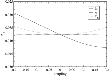
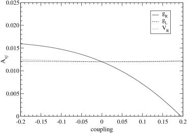
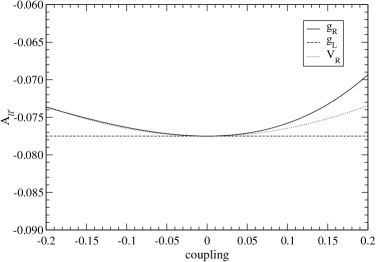
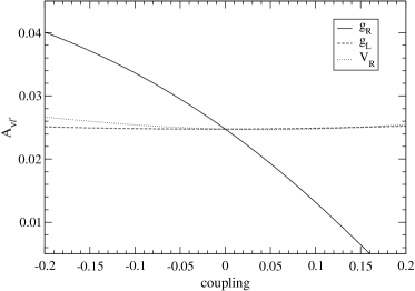
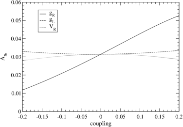
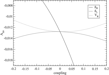
In the lepton ++ jets decay mode of the t​t¯𝑑¯𝑑t\bar{t} pair, t​t¯→ℓ​ν​b​j​j​bΒ―β†’π‘‘Β―π‘‘β„“πœˆπ‘π‘—π‘—Β―π‘t\bar{t}\to\ell\nu bjj\bar{b} we choose the two asymmetries Aℓ​jsubscript𝐴ℓ𝑗A_{\ell j}, Aν​jsubscriptπ΄πœˆπ‘—A_{\nu j}, for which we obtain the SM tree-level values Aℓ​j=βˆ’0.0376subscript𝐴ℓ𝑗0.0376A_{\ell j}=-0.0376, Aν​j=0.0120subscriptπ΄πœˆπ‘—0.0120A_{\nu j}=0.0120. With the precision expected for their measurement at LHC [16], the measurements Aℓ​jβ‰ƒβˆ’0.0376Β±0.0058similar-to-or-equalssubscript𝐴ℓ𝑗plus-or-minus0.03760.0058A_{\ell j}\simeq-0.0376\pm 0.0058, Aν​j≃0.0120Β±0.0056similar-to-or-equalssubscriptπ΄πœˆπ‘—plus-or-minus0.01200.0056A_{\nu j}\simeq 0.0120\pm 0.0056 are feasible. The dependence of these asymmetries on anomalous W​t​bπ‘Šπ‘‘π‘Wtb couplings is depicted in Fig.Β 6 (we remind the reader that the y𝑦y axis scales are chosen so that the range approximately corresponds to two standard deviations around the theoretical SM value). These plots are obtained using Eqs.Β (16),(20). We have checked, using high-statistics Monte Carlo simulations, that finite width effects are rather small, so that Eqs.Β (16),(20) can be used to make accurate predictions for spin correlation asymmetries. In the dilepton channel t​t¯→ℓ​ν​b​ℓ′​ν​bΒ―β†’π‘‘Β―π‘‘β„“πœˆπ‘superscriptβ„“β€²πœˆΒ―π‘t\bar{t}\to\ell\nu b\ell^{\prime}\nu\bar{b} we select the asymmetries Aℓ​ℓ′subscript𝐴ℓsuperscriptβ„“β€²A_{\ell\ell^{\prime}}, Aν​ℓ′subscript𝐴𝜈superscriptβ„“β€²A_{\nu\ell^{\prime}}, whose SM values are Aℓ​ℓ′=βˆ’0.0775subscript𝐴ℓsuperscriptβ„“β€²0.0775A_{\ell\ell^{\prime}}=-0.0775, Aν​ℓ′=0.0247subscript𝐴𝜈superscriptβ„“β€²0.0247A_{\nu\ell^{\prime}}=0.0247. The uncertainty in their measurement can be estimated from Refs.Β [19, 16], yielding Aβ„“β€‹β„“β€²β‰ƒβˆ’0.0775Β±0.0060similar-to-or-equalssubscript𝐴ℓsuperscriptβ„“β€²plus-or-minus0.07750.0060A_{\ell\ell^{\prime}}\simeq-0.0775\pm 0.0060, Aν​ℓ′≃0.0247Β±0.0087similar-to-or-equalssubscript𝐴𝜈superscriptβ„“β€²plus-or-minus0.02470.0087A_{\nu\ell^{\prime}}\simeq 0.0247\pm 0.0087. Their variation when anomalous couplings are present is shown in Fig.Β 6. We also plot (in this case with arbitrary y𝑦y axis scales) the asymmetries Al​bsubscript𝐴𝑙𝑏A_{lb}, Ab​bsubscript𝐴𝑏𝑏A_{bb}, which can be measured either in the semileptonic or dilepton channel. Their SM values are Al​b=0.0314subscript𝐴𝑙𝑏0.0314A_{lb}=0.0314, Ab​b=βˆ’0.0128subscript𝐴𝑏𝑏0.0128A_{bb}=-0.0128, but the experimental sensitivity has been not estimated as yet. We expect that it may be of the order of 10% for Al​bsubscript𝐴𝑙𝑏A_{lb}, and worse for Ab​bsubscript𝐴𝑏𝑏A_{bb}.

Refer to caption Refer to caption
Figure 6: Dependence of several spin correlation asymmetries on the couplings gRsubscript𝑔𝑅g_{R}, gLsubscript𝑔𝐿g_{L} and VRsubscript𝑉𝑅V_{R}, for the CP-conserving case.

The comparison of these plots with the ones in previous sections makes apparent that, given the experimental accuracies achievable in each case, spin correlation asymmetries are much less sensitive to non-standard W​t​bπ‘Šπ‘‘π‘Wtb couplings. This implies that, if no deviations are found in the measurement of the helicity ratios ρR,LsubscriptπœŒπ‘…πΏ\rho_{R,L} and angular asymmetries AΒ±subscript𝐴plus-or-minusA_{\pm}, spin-dependent asymmetries can be used to test t​t¯𝑑¯𝑑t\bar{t} spin correlations in the production, without contamination from possible new interactions in the decay. In particular, this is the case of Aℓ​ℓ′subscript𝐴ℓsuperscriptβ„“β€²A_{\ell\ell^{\prime}} and Aℓ​jsubscript𝐴ℓ𝑗A_{\ell j}, whose relative accuracy is better, 7.7% and 15%, respectively. The determination of the correlation factor C𝐢C in Eq.Β (18) from these asymmetries would eventually give

Aℓ​ℓ′subscript𝐴ℓsuperscriptβ„“β€²\displaystyle A_{\ell\ell^{\prime}} β†’β†’\displaystyle\rightarrow C=0.310Β±0.024(exp)(Ξ΄VR)βˆ’0.0043+0.(Ξ΄gL)βˆ’3Γ—10βˆ’6+1Γ—10βˆ’5(Ξ΄gR)βˆ’0.0004+7Γ—10βˆ’6,\displaystyle C=0.310\pm 0.024~{}\text{(exp)}~{}^{+0.}_{-0.0043}~{}(\delta V_{R})~{}^{+1\times 10^{-5}}_{-3\times 10^{-6}}~{}(\delta g_{L})~{}^{+7\times 10^{-6}}_{-0.0004}~{}(\delta g_{R})\,,
Aℓ​jsubscript𝐴ℓ𝑗\displaystyle A_{\ell j} β†’β†’\displaystyle\rightarrow C=0.310Β±0.045(exp)(Ξ΄VR)βˆ’0.0068+0.(Ξ΄gL)βˆ’0.0008+0.0001(Ξ΄gR)βˆ’0.0009+0.0004.\displaystyle C=0.310\pm 0.045~{}\text{(exp)}~{}^{+0.}_{-0.0068}~{}(\delta V_{R})~{}^{+0.0001}_{-0.0008}~{}(\delta g_{L})~{}^{+0.0004}_{-0.0009}~{}(\delta g_{R})\,. (21)

The first error quoted corresponds to the experimental (systematic and statistic) uncertainty. The other ones are theoretical uncertainties obtained varying the anomalous couplings (one at a time). The confidence level (CL) corresponding to the intervals quoted is 68.3%. The numerical comparison of the different terms in Eqs.Β (21) also shows that Aℓ​jsubscript𝐴ℓ𝑗A_{\ell j} and Aℓ​ℓ′subscript𝐴ℓsuperscriptβ„“β€²A_{\ell\ell^{\prime}} are much less sensitive to non-standard top couplings than A+subscript𝐴A_{+}, Aβˆ’subscript𝐴A_{-} and ρR,LsubscriptπœŒπ‘…πΏ\rho_{R,L}. It must also be noted that, since all asymmetries depend on the production mechanism through the common factor C𝐢C, their ratios do not (to leading order), and hence they are clean probes for anomalous couplings. The precision in the measurement of asymmetry ratios is still to be determined, but at any rate it is expected to be worse than for spin-independent observables discussed in the previous sections.

It is also interesting to study the relative distribution of one spin analyser from the t𝑑t quark and other from the t¯¯𝑑\bar{t}. Let Ο†X​XΒ―β€²subscriptπœ‘π‘‹superscript¯𝑋′\varphi_{X\bar{X}^{\prime}} be the angle between the three-momentum of X𝑋X (in the t𝑑t rest frame) and of XΒ―β€²superscript¯𝑋′\bar{X}^{\prime} (in the t¯¯𝑑\bar{t} rest frame). The angular distribution can be written as [23]

1σ​d​σd​cos⁑φX​XΒ―β€²=12​(1+D​αX​αX¯′​cos⁑φX​XΒ―β€²),1πœŽπ‘‘πœŽπ‘‘subscriptπœ‘π‘‹superscript¯𝑋′121𝐷subscript𝛼𝑋subscript𝛼superscript¯𝑋′subscriptπœ‘π‘‹superscript¯𝑋′\frac{1}{\sigma}\frac{d\sigma}{d\cos\varphi_{X\bar{X}^{\prime}}}=\frac{1}{2}(1+D\,\alpha_{X}\alpha_{\bar{X}^{\prime}}\cos\varphi_{X\bar{X}^{\prime}})\,, (22)

with D𝐷D a constant defined by this equality. In our simulations we obtain the tree-level value D=βˆ’0.217𝐷0.217D=-0.217, while at one loop D=βˆ’0.238𝐷0.238D=-0.238 [23], with a theoretical uncertainty of ∼4similar-toabsent4\sim 4%. Corresponding to these distributions, we can build the asymmetries

A~X​X¯′≑N​(cos⁑φX​XΒ―β€²>0)βˆ’N​(cos⁑φX​XΒ―β€²<0)N​(cos⁑φX​XΒ―β€²>0)+N​(cos⁑φX​XΒ―β€²<0)=12​D​αX​αXΒ―β€².subscript~𝐴𝑋superscript¯𝑋′𝑁subscriptπœ‘π‘‹superscript¯𝑋′0𝑁subscriptπœ‘π‘‹superscript¯𝑋′0𝑁subscriptπœ‘π‘‹superscript¯𝑋′0𝑁subscriptπœ‘π‘‹superscript¯𝑋′012𝐷subscript𝛼𝑋subscript𝛼superscript¯𝑋′\tilde{A}_{X\bar{X}^{\prime}}\equiv\frac{N(\cos\varphi_{X\bar{X}^{\prime}}>0)-N(\cos\varphi_{X\bar{X}^{\prime}}<0)}{N(\cos\varphi_{X\bar{X}^{\prime}}>0)+N(\cos\varphi_{X\bar{X}^{\prime}}<0)}=\frac{1}{2}D\alpha_{X}\alpha_{\bar{X}^{\prime}}\,. (23)

For charge conjugate decay channels the distributions can be summed, since Ξ±X′​αXΒ―=Ξ±X​αXΒ―β€²subscript𝛼superscript𝑋′subscript𝛼¯𝑋subscript𝛼𝑋subscript𝛼superscript¯𝑋′\alpha_{X^{\prime}}\alpha_{\bar{X}}=\alpha_{X}\alpha_{\bar{X}^{\prime}} provided CP is conserved in the decay. The dependence of these asymmetries A~X​XΒ―β€²subscript~𝐴𝑋superscript¯𝑋′\tilde{A}_{X\bar{X}^{\prime}} on anomalous couplings is (within the production Γ—\times decay factorisation approximation) exactly the same as for the asymmetries AX​XΒ―β€²subscript𝐴𝑋superscript¯𝑋′A_{X\bar{X}^{\prime}} defined above, and plots are not presented for brevity. Simulations are available for A~ℓ​jsubscript~𝐴ℓ𝑗\tilde{A}_{\ell j} and A~ℓ​ℓ′subscript~𝐴ℓsuperscriptβ„“β€²\tilde{A}_{\ell\ell^{\prime}}, whose theoretical SM values are A~ℓ​j=0.0527subscript~𝐴ℓ𝑗0.0527\tilde{A}_{\ell j}=0.0527, A~ℓ​ℓ′=0.1085subscript~𝐴ℓsuperscriptβ„“β€²0.1085\tilde{A}_{\ell\ell^{\prime}}=0.1085. The experimental precision expected [16, 19] is A~ℓ​j≃0.0554Β±0.0061similar-to-or-equalssubscript~𝐴ℓ𝑗plus-or-minus0.05540.0061\tilde{A}_{\ell j}\simeq 0.0554\pm 0.0061, A~ℓ​ℓ′≃0.1088Β±0.0056similar-to-or-equalssubscript~𝐴ℓsuperscriptβ„“β€²plus-or-minus0.10880.0056\tilde{A}_{\ell\ell^{\prime}}\simeq 0.1088\pm 0.0056. This is a better precision than for Aℓ​jsubscript𝐴ℓ𝑗A_{\ell j} and Aℓ​jsubscript𝐴ℓ𝑗A_{\ell j}, respectively, but still not competitive in the determination of the W​t​bπ‘Šπ‘‘π‘Wtb vertex structure.555A special situation occurs if there is a fine-tuned cancellation between two nonzero VRsubscript𝑉𝑅V_{R} and gLsubscript𝑔𝐿g_{L} couplings leading to small effects in Wπ‘ŠW helicity fractions and related quantities. These cancellations are possible, and in such particular case the measurement of spin asymmetries like Aℓ​ℓ′subscript𝐴ℓsuperscriptβ„“β€²A_{\ell\ell^{\prime}} and A~ℓ​ℓ′subscript~𝐴ℓsuperscriptβ„“β€²\tilde{A}_{\ell\ell^{\prime}} (which are insensitive to gLsubscript𝑔𝐿g_{L} but sensitive to VRsubscript𝑉𝑅V_{R}) or single top production may be used to obtain additional information about anomalous W​t​bπ‘Šπ‘‘π‘Wtb couplings. Instead, we can use them to test top spin correlations. From these asymmetries one can extract the value of D𝐷D, obtaining

A~ℓ​ℓ′subscript~𝐴ℓsuperscriptβ„“β€²\displaystyle\tilde{A}_{\ell\ell^{\prime}} β†’β†’\displaystyle\rightarrow D=βˆ’0.217Β±0.011(exp)(Ξ΄VR)βˆ’0.+0.0031(Ξ΄gL)βˆ’8Γ—10βˆ’6+2Γ—10βˆ’6(Ξ΄gR)βˆ’0.+0.0003,\displaystyle D=-0.217\pm 0.011~{}\text{(exp)}~{}^{+0.0031}_{-0.}~{}(\delta V_{R})~{}^{+2\times 10^{-6}}_{-8\times 10^{-6}}~{}(\delta g_{L})~{}^{+0.0003}_{-0.}~{}(\delta g_{R})\,,
A~ℓ​jsubscript~𝐴ℓ𝑗\displaystyle\tilde{A}_{\ell j} β†’β†’\displaystyle\rightarrow D=βˆ’0.217Β±0.024(exp)(Ξ΄VR)βˆ’0.+0.0047(Ξ΄gL)βˆ’9Γ—10βˆ’6+0.0006(Ξ΄gR)βˆ’6Γ—10βˆ’5+0.0004.\displaystyle D=-0.217\pm 0.024~{}\text{(exp)}~{}^{+0.0047}_{-0.}~{}(\delta V_{R})~{}^{+0.0006}_{-9\times 10^{-6}}~{}(\delta g_{L})~{}^{+0.0004}_{-6\times 10^{-5}}~{}(\delta g_{R})\,.

The errors quoted correspond to the experimental (systematic + statistical) uncertainty and the variation when one of the anomalous couplings is allowed to be nonzero. As in the previous case, the measurement of a ratio of two asymmetries A~X​XΒ―β€²subscript~𝐴𝑋superscript¯𝑋′\tilde{A}_{X\bar{X}^{\prime}} provides a clean probe for anomalous couplings, but with a precision expected to be worse than for spin-independent observables.

6 Effect of complex phases in helicity fractions and spin asymmetries

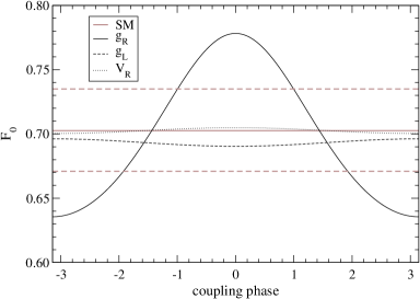
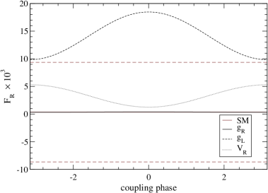
In the previous sections we have assumed that any non-standard W​t​bπ‘Šπ‘‘π‘Wtb couplings are real, either positive or negative. We have also pointed out that, if a non-zero coupling gRsubscript𝑔𝑅g_{R} exists, its phase has an important influence on Wπ‘ŠW helicity fractions and angular distributions determined by them. Complex phases in VRsubscript𝑉𝑅V_{R}, gLsubscript𝑔𝐿g_{L} and gRsubscript𝑔𝑅g_{R} influence the helicity fractions Fisubscript𝐹𝑖F_{i} through interference terms, which involve the real parts of these couplings (assuming VLsubscript𝑉𝐿V_{L} real). (Interference terms are the most important ones for small values of VRsubscript𝑉𝑅V_{R}, gLsubscript𝑔𝐿g_{L} and gRsubscript𝑔𝑅g_{R}, and for the latter coupling they are unsuppressed.) The maximum and minimum effects of anomalous couplings on Fisubscript𝐹𝑖F_{i} are obtained when they are real, negative or positive (not necessarily in this order). We show in Fig.Β 7 the values of the helicity fractions for fixed moduli and arbitrary phases of the new couplings, VR=0.1​ei​ϕVRsubscript𝑉𝑅0.1superscript𝑒𝑖subscriptitalic-Ο•subscript𝑉𝑅V_{R}=0.1\,e^{i\phi_{V_{R}}}, gL=0.1​ei​ϕgLsubscript𝑔𝐿0.1superscript𝑒𝑖subscriptitalic-Ο•subscript𝑔𝐿g_{L}=0.1\,e^{i\phi_{g_{L}}}, gR=0.1​ei​ϕgRsubscript𝑔𝑅0.1superscript𝑒𝑖subscriptitalic-Ο•subscript𝑔𝑅g_{R}=0.1\,e^{i\phi_{g_{R}}} (one different from zero at a time), to illustrate the effect of the phases. The plot scales have been enlarged to cover all the range of variation of Fisubscript𝐹𝑖F_{i}, and the 2​σ2𝜎2\sigma expected limits have been marked with a gray dashed line.
Refer to caption Refer to caption
Refer to caption
Figure 7: Dependence of the helicity fractions Fisubscript𝐹𝑖F_{i} on the phases of the anomalous couplings (see the text for details).

For gLsubscript𝑔𝐿g_{L} and VRsubscript𝑉𝑅V_{R} the deviations from the SM value are relatively stable under variations of the phases, because the linear terms (which depend on the phase) and quadratic ones (which do not) are comparable in magnitude. Thus, the presence of a complex phase does not significantly affect the observability of the coupling. On the other hand, for gRsubscript𝑔𝑅g_{R} the effect of the phase is dominant, and we notice that for phases Ο•gR=Β±Ο€/2subscriptitalic-Ο•subscript𝑔𝑅plus-or-minusπœ‹2\phi_{g_{R}}=\pm\pi/2 the helicity fractions are very close to their SM values, so that a purely imaginary coupling gR∼O​(0.1)similar-tosubscript𝑔𝑅𝑂0.1g_{R}\sim O(0.1) could remain unnoticed in an analysis of angular distributions. We also note that the plots are symmetric with respect to the y𝑦y axis, because Fisubscript𝐹𝑖F_{i} depend on Re​VRResubscript𝑉𝑅\text{Re}\,V_{R}, Re​gLResubscript𝑔𝐿\text{Re}\,g_{L}, Re​gRResubscript𝑔𝑅\text{Re}\,g_{R} and the moduli. This also implies that complex couplings have the same effect on the helicity fractions in t𝑑t and t¯¯𝑑\bar{t} decays. Therefore, the comparison in t𝑑t and t¯¯𝑑\bar{t} decays of the angular distributions studied does not give any extra information regarding the complex phases, and further observables are needed in order to investigate this possibility. We have also analysed the phase dependence of the most interesting spin asymmetries, Aℓ​jsubscript𝐴ℓ𝑗A_{\ell j}, A~ℓ​jsubscript~𝐴ℓ𝑗\tilde{A}_{\ell j}, Aℓ​ℓ′subscript𝐴ℓsuperscriptβ„“β€²A_{\ell\ell^{\prime}} and A~ℓ​ℓ′subscript~𝐴ℓsuperscriptβ„“β€²\tilde{A}_{\ell\ell^{\prime}} (in semileptonic decays we consider W+β†’β„“+​ν→superscriptπ‘Šsuperscriptβ„“πœˆW^{+}\to\ell^{+}\nu, Wβˆ’β†’q¯​qβ€²β†’superscriptπ‘ŠΒ―π‘žsuperscriptπ‘žβ€²W^{-}\to\bar{q}q^{\prime}). The effect of the phases is barely detectable, even with a greater experimental precision, and in any case the phase and modulus of an eventual anomalous coupling measured could not be disentangled.

7 CP-violating asymmetries

In this section we examine whether the existence of complex phases in the anomalous couplings can be detected using CP-violating asymmetries. The possibility of a relatively large imaginary coupling gRsubscript𝑔𝑅g_{R} is particularly intriguing, since angular distributions are very sensitive to this coupling provided its phase is not close to Β±Ο€/2plus-or-minusπœ‹2\pm\pi/2. For the other couplings, gLsubscript𝑔𝐿g_{L} and VRsubscript𝑉𝑅V_{R}, the situation is not so dramatic, because the observability mainly depends on their moduli.

The spin asymmetry [30]

AC​PR​L=σ​(tR​tΒ―R)βˆ’Οƒβ€‹(tL​tΒ―L)σ​(tR​tΒ―R)+σ​(tL​tΒ―L),superscriptsubscriptπ΄πΆπ‘ƒπ‘…πΏπœŽsubscript𝑑𝑅subscriptΒ―π‘‘π‘…πœŽsubscript𝑑𝐿subscriptΒ―π‘‘πΏπœŽsubscript𝑑𝑅subscriptΒ―π‘‘π‘…πœŽsubscript𝑑𝐿subscript¯𝑑𝐿A_{CP}^{RL}=\frac{\sigma(t_{R}\bar{t}_{R})-\sigma(t_{L}\bar{t}_{L})}{\sigma(t_{R}\bar{t}_{R})+\sigma(t_{L}\bar{t}_{L})}\,, (25)

is CP-violating, and vanishes at the tree level in QCD interactions. The top and antitop spins can be inferred using their decay products as spin analysers, in the same way as in section 5. We thus write

AC​PR​L=N​(cos⁑θX>0,cos⁑θXΒ―β€²>0)βˆ’N​(cos⁑θX<0,cos⁑θXΒ―β€²<0)N​(cos⁑θX>0,cos⁑θXΒ―β€²>0)+N​(cos⁑θX<0,cos⁑θXΒ―β€²<0).superscriptsubscript𝐴𝐢𝑃𝑅𝐿𝑁formulae-sequencesubscriptπœƒπ‘‹0subscriptπœƒsuperscript¯𝑋′0𝑁formulae-sequencesubscriptπœƒπ‘‹0subscriptπœƒsuperscript¯𝑋′0𝑁formulae-sequencesubscriptπœƒπ‘‹0subscriptπœƒsuperscript¯𝑋′0𝑁formulae-sequencesubscriptπœƒπ‘‹0subscriptπœƒsuperscript¯𝑋′0A_{CP}^{RL}=\frac{N(\cos\theta_{X}>0,\cos\theta_{\bar{X}^{\prime}}>0)-N(\cos\theta_{X}<0,\cos\theta_{\bar{X}^{\prime}}<0)}{N(\cos\theta_{X}>0,\cos\theta_{\bar{X}^{\prime}}>0)+N(\cos\theta_{X}<0,\cos\theta_{\bar{X}^{\prime}}<0)}\,. (26)

Even with AC​PL​Rsuperscriptsubscript𝐴𝐢𝑃𝐿𝑅A_{CP}^{LR} vanishing in the production process, complex phases in the decay could in principle lead to an observable asymmetry. We have considered the dilepton channel, in which larger asymmetries are expected because of the higher spin analysing power of the charged leptons. (Other possibility to measure this asymmetry in the dilepton channel would be to consider the charged lepton energies [31].) We have found that, for anomalous couplings of order O​(0.1)𝑂0.1O(0.1) and arbitrary phases, this asymmetry remains below the permille level, and with values consistent with zero within Monte Carlo uncertainty. Observation of such asymmetry would then unambiguously indicate CP-violating effects in t​t¯𝑑¯𝑑t\bar{t} production, which are possible, for instance, in two Higgs doublet models [30, 32, 33].

We also investigate triple-product asymmetries defined in the dilepton channel,

AC​PTi=N​(Ti>0)βˆ’N​(Ti<0)N​(Ti>0)+N​(Ti<0),superscriptsubscript𝐴𝐢𝑃subscript𝑇𝑖𝑁subscript𝑇𝑖0𝑁subscript𝑇𝑖0𝑁subscript𝑇𝑖0𝑁subscript𝑇𝑖0A_{CP}^{T_{i}}=\frac{N(T_{i}>0)-N(T_{i}<0)}{N(T_{i}>0)+N(T_{i}<0)}\,, (27)

where the triple products Tisubscript𝑇𝑖T_{i} are [32, 34]

T1subscript𝑇1\displaystyle T_{1} =\displaystyle= e^β‹…(pβ†’β„“+βˆ’pβ†’β„“βˆ’)​(pβ†’β„“+Γ—pβ†’β„“βˆ’)β‹…e^,β‹…β‹…^𝑒subscript→𝑝superscriptβ„“subscript→𝑝superscriptβ„“subscript→𝑝superscriptβ„“subscript→𝑝superscriptβ„“^𝑒\displaystyle\hat{e}\cdot(\vec{p}_{\ell^{+}}-\vec{p}_{\ell^{-}})\;(\vec{p}_{\ell^{+}}\times\vec{p}_{\ell^{-}})\cdot\hat{e}\,,
T2subscript𝑇2\displaystyle T_{2} =\displaystyle= (pβ†’bβˆ’pβ†’bΒ―)β‹…(pβ†’β„“+Γ—pβ†’β„“βˆ’),β‹…subscript→𝑝𝑏subscript→𝑝¯𝑏subscript→𝑝superscriptβ„“subscript→𝑝superscriptβ„“\displaystyle(\vec{p}_{b}-\vec{p}_{\bar{b}})\cdot(\vec{p}_{\ell^{+}}\times\vec{p}_{\ell^{-}})\,,
T3subscript𝑇3\displaystyle T_{3} =\displaystyle= (pβ†’tβˆ’pβ†’tΒ―)β‹…(pβ†’β„“+Γ—pβ†’β„“βˆ’).β‹…subscript→𝑝𝑑subscript→𝑝¯𝑑subscript→𝑝superscriptβ„“subscript→𝑝superscriptβ„“\displaystyle(\vec{p}_{t}-\vec{p}_{\bar{t}})\cdot(\vec{p}_{\ell^{+}}\times\vec{p}_{\ell^{-}})\,. (28)

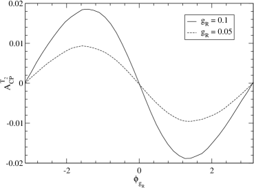
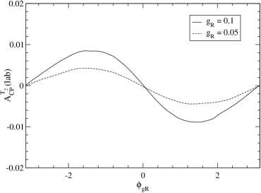
The unit vector e^^𝑒\hat{e} is taken in the beam direction and the particle momenta follow obvious notation. Final state particle momenta can be measured in the laboratory frame or, if the kinematics of the event is completely reconstructed, in other reference system. For asymmetries built using T1subscript𝑇1T_{1} and T3subscript𝑇3T_{3} we have found values O​(10βˆ’4)𝑂superscript104O(10^{-4}), and compatible with zero, taking anomalous couplings of order O​(0.1)𝑂0.1O(0.1) with arbitrary phases. On the other hand, we have found that AC​PT2superscriptsubscript𝐴𝐢𝑃subscript𝑇2A_{CP}^{T_{2}} is sensitive to a gRsubscript𝑔𝑅g_{R} coupling of this magnitude. The asymmetry is larger if the charged lepton and b𝑏b quark momenta are measured in the respective rest frames of the decaying top quarks. However, its observability will depend on systematic errors associated to the reconstruction, which have not been estimated as yet, and may be better when defined in the laboratory frame. The asymmetry AC​PT2superscriptsubscript𝐴𝐢𝑃subscript𝑇2A_{CP}^{T_{2}} in both reference systems as plotted in Fig.Β 8, for couplings gR=0.05subscript𝑔𝑅0.05g_{R}=0.05, gR=0.1subscript𝑔𝑅0.1g_{R}=0.1 with arbitrary phases.

Refer to caption Refer to caption
Figure 8: Dependence of the CP asymmetry AC​PT2superscriptsubscript𝐴𝐢𝑃subscript𝑇2A_{CP}^{T_{2}}, defined in top quark rest frame (left) and laboratory system (right), on the phase of gRsubscript𝑔𝑅g_{R}.

Other asymmetries discussed in the literature are based on the differences

Ξ”1subscriptΞ”1\displaystyle\Delta_{1} =\displaystyle= Eβ„“+βˆ’Eβ„“βˆ’,subscript𝐸superscriptβ„“subscript𝐸superscriptβ„“\displaystyle E_{\ell^{+}}-E_{\ell^{-}}\,,
Ξ”2subscriptΞ”2\displaystyle\Delta_{2} =\displaystyle= pβ†’tΒ―β‹…pβ†’β„“+βˆ’pβ†’tβ‹…pβ†’β„“βˆ’,β‹…subscript→𝑝¯𝑑subscript→𝑝superscriptβ„“β‹…subscript→𝑝𝑑subscript→𝑝superscriptβ„“\displaystyle\vec{p}_{\bar{t}}\cdot\vec{p}_{\ell^{+}}-\vec{p}_{t}\cdot\vec{p}_{\ell^{-}}\,,
Ξ”3subscriptΞ”3\displaystyle\Delta_{3} =\displaystyle= cos⁑θℓ+βˆ’cosβ‘ΞΈβ„“βˆ’.subscriptπœƒsuperscriptβ„“subscriptπœƒsuperscriptβ„“\displaystyle\cos\theta_{\ell^{+}}-\cos\theta_{\ell^{-}}\,. (29)

These quantities do not involve the product (pβ†’β„“+Γ—pβ†’β„“βˆ’)subscript→𝑝superscriptβ„“subscript→𝑝superscriptβ„“(\vec{p}_{\ell^{+}}\times\vec{p}_{\ell^{-}}), and then they can be measured in the semileptonic channel too [34]. The asymmetries are built as in Eq.Β (27), and take values below the permille level for anomalous couplings of the size considered in this section. For completeness, we have also considered the P-violating asymmetry

APR​L=σ​(tR​tΒ―L)βˆ’Οƒβ€‹(tL​tΒ―R)σ​(tR​tΒ―L)+σ​(tL​tΒ―R),superscriptsubscriptπ΄π‘ƒπ‘…πΏπœŽsubscript𝑑𝑅subscriptΒ―π‘‘πΏπœŽsubscript𝑑𝐿subscriptΒ―π‘‘π‘…πœŽsubscript𝑑𝑅subscriptΒ―π‘‘πΏπœŽsubscript𝑑𝐿subscript¯𝑑𝑅A_{P}^{RL}=\frac{\sigma(t_{R}\bar{t}_{L})-\sigma(t_{L}\bar{t}_{R})}{\sigma(t_{R}\bar{t}_{L})+\sigma(t_{L}\bar{t}_{R})}\,, (30)

which is measured using the charged leptons as spin analysers,

APR​L=N​(cos⁑θX>0,cos⁑θXΒ―β€²<0)βˆ’N​(cos⁑θX<0,cos⁑θXΒ―β€²>0)N​(cos⁑θX>0,cos⁑θXΒ―β€²<0)+N​(cos⁑θX<0,cos⁑θXΒ―β€²>0).superscriptsubscript𝐴𝑃𝑅𝐿𝑁formulae-sequencesubscriptπœƒπ‘‹0subscriptπœƒsuperscript¯𝑋′0𝑁formulae-sequencesubscriptπœƒπ‘‹0subscriptπœƒsuperscript¯𝑋′0𝑁formulae-sequencesubscriptπœƒπ‘‹0subscriptπœƒsuperscript¯𝑋′0𝑁formulae-sequencesubscriptπœƒπ‘‹0subscriptπœƒsuperscript¯𝑋′0A_{P}^{RL}=\frac{N(\cos\theta_{X}>0,\cos\theta_{\bar{X}^{\prime}}<0)-N(\cos\theta_{X}<0,\cos\theta_{\bar{X}^{\prime}}>0)}{N(\cos\theta_{X}>0,\cos\theta_{\bar{X}^{\prime}}<0)+N(\cos\theta_{X}<0,\cos\theta_{\bar{X}^{\prime}}>0)}\,. (31)

We have found APR​L∼1.5Γ—10βˆ’3similar-tosuperscriptsubscript𝐴𝑃𝑅𝐿1.5superscript103A_{P}^{RL}\sim 1.5\times 10^{-3}, and insensitive to anomalous couplings O​(0.1)𝑂0.1O(0.1). This asymmetry can be sizeable in SM extensions [35].

We finally emphasise that, even in the cases where they are insensitive to complex anomalous W​t​bπ‘Šπ‘‘π‘Wtb couplings, the CP-violating asymmetries studied here are still very useful to disentangle CP violation in the production and the decay. If these asymmetries are found to be non-vanishing, they clearly signal CP violation in t​t¯𝑑¯𝑑t\bar{t} production. On the other hand, the imaginary part of gRsubscript𝑔𝑅g_{R} can be probed using AC​PT2superscriptsubscript𝐴𝐢𝑃subscript𝑇2A_{CP}^{T_{2}}.

8 Summary

New physics, if it exists close to the electroweak scale, may manifest itself through non-standard top interactions. In this paper we have discussed top pair decays at LHC as a probe of the W​t​bπ‘Šπ‘‘π‘Wtb vertex. We have examined angular and energy distributions, as well as asymmetries, involving or not the top quark polarisation. Among the observables discussed, the best sensitivity to anomalous W​t​bπ‘Šπ‘‘π‘Wtb couplings is given by the Wπ‘ŠW helicity fractions Fi=Ξ“i/Ξ“subscript𝐹𝑖subscriptΓ𝑖ΓF_{i}=\Gamma_{i}/\Gamma, i=L,R,0𝑖𝐿𝑅0i=L,R,0, and related observables. We have obtained analytical expressions for Fisubscript𝐹𝑖F_{i}, for a general CP-violating W​t​bπ‘Šπ‘‘π‘Wtb vertex with the top quark and Wπ‘ŠW boson on their mass shell, and keeping a non-zero bottom quark mass. We have shown, comparing with exact numerical results, the high accuracy of this approximation when studying angular distributions. We have also pointed out the importance of keeping the bottom mass in the calculations, in contrast with previous studies in the literature.

Wπ‘ŠW helicity fractions can be extracted from a fit to the charged lepton angular distribution in Wπ‘ŠW rest frame. The same analysis can be used to determine the helicity ratios ρR,L=Ξ“R,L/Ξ“0subscriptπœŒπ‘…πΏsubscriptΓ𝑅𝐿subscriptΞ“0\rho_{R,L}=\Gamma_{R,L}/\Gamma_{0}, which are actually more sensitive to VRsubscript𝑉𝑅V_{R} and gLsubscript𝑔𝐿g_{L}-type anomalous couplings, given the experimental uncertainties (dominated by systematics already for a luminosity of 10 fb-1) associated to each observable. A simpler method to probe the W​t​bπ‘Šπ‘‘π‘Wtb vertex, without the need of a fit to the charged lepton distribution, is through angular asymmetries. We have introduced two new asymmetries A+subscript𝐴A_{+} and Aβˆ’subscript𝐴A_{-}, in addition to the ℓ​Wβ„“π‘Š\ell W (or ℓ​bℓ𝑏\ell b) forward-backward asymmetry AFBsubscript𝐴FBA_{\mathrm{FB}} previously studied [9]. These new asymmetries allow us to: (i) obtain more precise bounds on anomalous couplings than AFBsubscript𝐴FBA_{\mathrm{FB}}, comparable with those obtained from ρR,LsubscriptπœŒπ‘…πΏ\rho_{R,L} and Fisubscript𝐹𝑖F_{i}, and even better for a gRsubscript𝑔𝑅g_{R} coupling; (ii) determine the helicity fractions with a fair accuracy without fitting the charged lepton distribution. The Wπ‘ŠW helicity fractions determine the charged lepton energy distribution in top rest frame as well. Energy asymmetries can be built, but they are less suited for the study of anomalous couplings because the approximation of considering the top quark and Wπ‘ŠW boson on shell is worse, and experimental uncertainties on energy asymmetries are larger. The best limits found, using single measurements, are

βˆ’0.029≀VR≀0.099(ρR),formulae-sequence0.029subscript𝑉𝑅0.099subscriptπœŒπ‘…\displaystyle-0.029\leq V_{R}\leq 0.099\quad(\rho_{R})\,,
βˆ’0.046≀gL≀0.013(ρR),formulae-sequence0.046subscript𝑔𝐿0.013subscriptπœŒπ‘…\displaystyle-0.046\leq g_{L}\leq 0.013\quad(\rho_{R})\,,
βˆ’0.019≀gR≀0.018(A+).formulae-sequence0.019subscript𝑔𝑅0.018subscript𝐴\displaystyle-0.019\leq g_{R}\leq 0.018\quad(A_{+})\,. (32)

Limits can be improved by combining the measurements of AΒ±subscript𝐴plus-or-minusA_{\pm} and ρR,LsubscriptπœŒπ‘…πΏ\rho_{R,L}. The theoretical predictions for these and other observables have been implemented in a computer program TopFit, which allows to extract combined limits on anomalous couplings from a given set of observables, following the statistical approach outlined in appendix B. Detailed results including the correlation of the various observables (computed from Monte Carlo simulations) are beyond the scope of this paper, and have been presented elsewhere [15].

Spin correlations and spin-dependent asymmetries probe not only the W​t​bπ‘Šπ‘‘π‘Wtb interactions but also the dynamics of t​t¯𝑑¯𝑑t\bar{t} production. Their study is very interesting from a theoretical point of view, because they are sensitive to e.g. the exchange of a scalar particle in s𝑠s channel [36] or anomalous g​t​t𝑔𝑑𝑑gtt couplings [37]. It is then crucial to disentangle new physics in the production from possible anomalous W​t​bπ‘Šπ‘‘π‘Wtb couplings. This could be done, for instance, considering ratios of spin correlation asymmetries or, even better, using the strict bounds on anomalous couplings obtained from top decay angular distributions.

The dependence of spin correlation asymmetries on W​t​bπ‘Šπ‘‘π‘Wtb anomalous couplings occurs through the β€œspin analysing power” constants of top quark decay products. We have calculated these constants for a general CP-conserving W​t​bπ‘Šπ‘‘π‘Wtb vertex, in the narrow width approximation. It has been shown that the sensitivity of spin correlation asymmetries to top anomalous couplings is much weaker than for helicity fractions and related observables. Then, we have set explicit limits on the variation of two factors C𝐢C, D𝐷D (which measure the t​t¯𝑑¯𝑑t\bar{t} spin correlation) due to possible anomalous couplings not detected in other processes, i.e. within the ranges in Eqs.Β (32). The possible variation in C𝐢C, D𝐷D is much smaller than the experimental precision expected for their measurement,

C𝐢\displaystyle C =0.310Β±0.024(exp)(Ξ΄VR)βˆ’0.0043+0.(Ξ΄gL)βˆ’3Γ—10βˆ’6+1Γ—10βˆ’5(Ξ΄gR)βˆ’0.0004+7Γ—10βˆ’6,\displaystyle=0.310\pm 0.024~{}\text{(exp)}~{}^{+0.}_{-0.0043}~{}(\delta V_{R})~{}^{+1\times 10^{-5}}_{-3\times 10^{-6}}~{}(\delta g_{L})~{}^{+7\times 10^{-6}}_{-0.0004}~{}(\delta g_{R})\,,
D𝐷\displaystyle D =βˆ’0.217Β±0.011(exp)(Ξ΄VR)βˆ’0.+0.0047(Ξ΄gL)βˆ’9Γ—10βˆ’6+0.0006(Ξ΄gR)βˆ’6Γ—10βˆ’5+0.0004.\displaystyle=-0.217\pm 0.011~{}\text{(exp)}~{}^{+0.0047}_{-0.}~{}(\delta V_{R})~{}^{+0.0006}_{-9\times 10^{-6}}~{}(\delta g_{L})~{}^{+0.0004}_{-6\times 10^{-5}}~{}(\delta g_{R})\,. (33)

Hence, any deviation observed experimentally should correspond to new physics in the production. On the other hand, in ratios of two spin asymmetries AX​XΒ―β€²subscript𝐴𝑋superscript¯𝑋′A_{X\bar{X}^{\prime}} (A~X​XΒ―β€²subscript~𝐴𝑋superscript¯𝑋′\tilde{A}_{X\bar{X}^{\prime}}) the common factors C𝐢C (D𝐷D) cancel, and thus the ratios can cleanly probe non-standard top couplings. These observables have also been implemented in the computer program TopFit, and estimates for their expected precision will be presented elsewhere.

Finally, we have addressed the possibility of complex anomalous W​t​bπ‘Šπ‘‘π‘Wtb couplings gLsubscript𝑔𝐿g_{L}, gRsubscript𝑔𝑅g_{R}, VRsubscript𝑉𝑅V_{R}. Complex phases in these terms influence helicity fractions and related quantities via the interference with the dominant SM coupling VLsubscript𝑉𝐿V_{L} (which we have normalised to unity). For VRsubscript𝑉𝑅V_{R} and gLsubscript𝑔𝐿g_{L}, quadratic and interference terms have the same magnitude, and the effect of phases is not very relevant. For gRsubscript𝑔𝑅g_{R}, however, the interference term dominates, and the dependence on the phase is very strong. One finds that a gRsubscript𝑔𝑅g_{R} coupling with a phase close to Β±Ο€/2plus-or-minusπœ‹2\pm\pi/2 has little effect on angular distributions, and even with a relatively large modulus it could remain unnoticed in such analyses. The same has been found for spin correlation asymmetries. However, we have shown that a CP asymmetry based on the triple product (pβ†’bβˆ’pβ†’bΒ―)β‹…(pβ†’β„“+Γ—pβ†’β„“βˆ’)β‹…subscript→𝑝𝑏subscript→𝑝¯𝑏subscript→𝑝superscriptβ„“subscript→𝑝superscriptβ„“(\vec{p}_{b}-\vec{p}_{\bar{b}})\cdot(\vec{p}_{\ell^{+}}\times\vec{p}_{\ell^{-}}) is sensitive to a complex gRsubscript𝑔𝑅g_{R}, taking values up to Β±2plus-or-minus2\pm 2% for gR=βˆ“0.1​isubscript𝑔𝑅minus-or-plus0.1𝑖g_{R}=\mp 0.1i. If this asymmetry can be measured at LHC with a precision below the percent level, it could help to measure or bound gRsubscript𝑔𝑅g_{R}. The remaining CP asymmetries analysed are very small, and insensitive to anomalous couplings of this size. Therefore, they can be used to isolate CP violating effects in t​t¯𝑑¯𝑑t\bar{t} production [32, 33]. On the other hand, single top production at LHC can probe the W​t​bπ‘Šπ‘‘π‘Wtb interaction, and B𝐡B or super-B𝐡B factories, with precise measurements of CP asymmetries e.g. in bβ†’s​γ→𝑏𝑠𝛾b\to s\gamma, might also give indirect evidence for (real or complex) anomalous W​t​bπ‘Šπ‘‘π‘Wtb couplings, helping to determine the structure of this vertex.

Acknowledgements

The work of J.A.A.-S. has been supported by a MEC Ramon y Cajal contract and project FPA2003–09298–C02–01, and by Junta de AndalucΓ­a through project FQM-101. The work of J.C., N.C. (grant SFRH/BD/13936/2003), A.O. and F.V. (grant SFRH/BD/ 18762/2004) has been supported by Funda Γ£o para a CiΓͺncia e a Tecnologia.

Appendix A Effect of π’Žπ’ƒsubscriptπ’Žπ’ƒ\boldsymbol{m_{b}} in the helicity fractions

As it can be observed in Eqs.Β (2), interference terms involving VRsubscript𝑉𝑅V_{R} (or gLsubscript𝑔𝐿g_{L}) and the dominant SM coupling VLsubscript𝑉𝐿V_{L} are proportional to xb=mb/mtsubscriptπ‘₯𝑏subscriptπ‘šπ‘subscriptπ‘šπ‘‘x_{b}=m_{b}/m_{t}. These terms are of equal size as the quadratic terms for small VRsubscript𝑉𝑅V_{R}, gLsubscript𝑔𝐿g_{L}, and cannot be neglected in the analysis. To illustrate their importance, we plot in Fig.Β 9 the dependence of the three helicity fractions on the anomalous couplings, for mb=4.8subscriptπ‘šπ‘4.8m_{b}=4.8 GeV and neglecting mbsubscriptπ‘šπ‘m_{b}. The differences are apparent for FRsubscript𝐹𝑅F_{R}, and for F0subscript𝐹0F_{0} we have the extreme situation that the only dependence of this quantity on VRsubscript𝑉𝑅V_{R} is through the xbsubscriptπ‘₯𝑏x_{b} term.

Refer to caption Refer to caption
Refer to caption
Figure 9: Dependence of the helicity fractions Fisubscript𝐹𝑖F_{i} on VRsubscript𝑉𝑅V_{R} and gLsubscript𝑔𝐿g_{L}, for mb=4.8subscriptπ‘šπ‘4.8m_{b}=4.8 GeV and neglecting the b𝑏b quark mass.

The mbsubscriptπ‘šπ‘m_{b} dependence of the limits generates a small uncertainty due to the uncertainty in mbsubscriptπ‘šπ‘m_{b}, for which we use the b𝑏b quark pole mass. This b𝑏b mass definition has an ambiguity of the order of Ξ›QCD≃220similar-to-or-equalssubscriptΞ›QCD220\Lambda_{\mathrm{QCD}}\simeq 220 MeV (for other definitions the uncertainty is smaller). The variation of the limits in Eq.Β (32) when mbsubscriptπ‘šπ‘m_{b} is taken as 4.8 GeV Β±Ξ›QCDplus-or-minussubscriptΞ›QCD\pm\Lambda_{\mathrm{QCD}} is presented in TableΒ 4 (we display additional digits in order to better illustrate the variation). The effect is larger for VRsubscript𝑉𝑅V_{R} and gLsubscript𝑔𝐿g_{L}, as it is expected from the discussion in section 2. Nevertheless, the uncertainty only amounts to a few percent.

Lower limit Upper limit
Coupling mbβˆ’Ξ›QCDsubscriptπ‘šπ‘subscriptΞ›QCDm_{b}-\Lambda_{\mathrm{QCD}} mbsubscriptπ‘šπ‘m_{b} mb+Ξ›QCDsubscriptπ‘šπ‘subscriptΞ›QCDm_{b}+\Lambda_{\mathrm{QCD}} mbβˆ’Ξ›QCDsubscriptπ‘šπ‘subscriptΞ›QCDm_{b}-\Lambda_{\mathrm{QCD}} mbsubscriptπ‘šπ‘m_{b} mb+Ξ›QCDsubscriptπ‘šπ‘subscriptΞ›QCDm_{b}+\Lambda_{\mathrm{QCD}}
VRsubscript𝑉𝑅V_{R} -0.0303 -0.0293 -0.0281 0.0977 0.0994 0.1077
gLsubscript𝑔𝐿g_{L} -0.0444 -0.0456 -0.0461 0.0140 0.0135 0.0127
gRsubscript𝑔𝑅g_{R} -0.0192 -0.0194 -0.0192 0.0181 0.0180 0.0178
Table 4: Influence of mbsubscriptπ‘šπ‘m_{b} in the limits in Eqs.Β (32): variation when the b𝑏b quark mass is taken at its central value mb=4.8subscriptπ‘šπ‘4.8m_{b}=4.8 GeV, or adding and subtracting a small uncertainty Ξ›QCD=220subscriptΞ›QCD220\Lambda_{\mathrm{QCD}}=220 MeV.

Appendix B Extraction of limits from observables

The derivation of limits on the anomalous couplings from the measurement of the experimental observables discussed has to be done with special care, due to the non-linear dependence of the latter on the former. In this appendix we explain the method we have used to obtain our limits.

Let us denote by O𝑂O a generic observable, e.g. an angular asymmetry, and xπ‘₯x an unknown parameter (in our case an anomalous coupling) upon which this observable depends, and for which we want to obtain a confidence interval. O𝑂O is experimentally measured and is assumed to obey a Gaussian distribution (with mean and standard deviation given by its measurement). However, if the dependence O​(x)𝑂π‘₯O(x) is non-linear in the region of interest, the probability density function (p.d.f.) derived for the parameter xπ‘₯x will no longer be a Gaussian and a Monte Carlo method must be used to determine a confidence interval on xπ‘₯x.

We determine the p.d.f. of xπ‘₯x numerically, using the acceptance-rejection method: we iteratively (i) generate a random value (with uniform probability) xisubscriptπ‘₯𝑖x_{i} within a suitable interval; (ii) evaluate the probability of O​(xi)𝑂subscriptπ‘₯𝑖O(x_{i}), given by the p.d.f. of O𝑂O; (iii) generate an independent random number risubscriptπ‘Ÿπ‘–r_{i} (with uniform probability); and (iv) accept the value xisubscriptπ‘₯𝑖x_{i} if the probability of O​(xi)𝑂subscriptπ‘₯𝑖O(x_{i}) is larger than risubscriptπ‘Ÿπ‘–r_{i}. The resulting set of values {xi}subscriptπ‘₯𝑖\{x_{i}\} is distributed according to the p.d.f. of xπ‘₯x given by the measurement of O𝑂O. The determination of a central interval with a given confidence level (CL) γ𝛾\gamma is done numerically, requiring: (a) that it contains a fraction γ𝛾\gamma of the total number of values {xi}subscriptπ‘₯𝑖\{x_{i}\}; (b) that is central, i.e. fractions (1βˆ’Ξ³)/21𝛾2(1-\gamma)/2 of the values generated are on each side of the interval.

We have applied this method to obtain the limits on TablesΒ 1 and 2, keeping only one of the couplings non-vanishing at a time. We point out that:

  1. 1.

    The dependence on gRsubscript𝑔𝑅g_{R} of the observables Fisubscript𝐹𝑖F_{i}, ρR,LsubscriptπœŒπ‘…πΏ\rho_{R,L}, AΒ±subscript𝐴plus-or-minusA_{\pm} and AFBsubscript𝐴FBA_{\mathrm{FB}} is approximately linear, as it can be observed in Figs.Β 2–4. Therefore, the limits on this coupling can be approximately obtained directly from these plots using the method in Refs.Β [19, 16]: for a given observable O𝑂O, intersecting the plot of O​(gR)𝑂subscript𝑔𝑅O(g_{R}) with the two horizontal lines O=Oexp±Δ​O𝑂plus-or-minussubscript𝑂expΔ𝑂O=O_{\text{exp}}\pm\Delta O, which correspond to the 1​σ1𝜎1\sigma variation of O𝑂O, gives the 1​σ1𝜎1\sigma interval (with a 68.3% CL) on gRsubscript𝑔𝑅g_{R}.

  2. 2.

    The dependence on gLsubscript𝑔𝐿g_{L} and VLsubscript𝑉𝐿V_{L} is highly non-linear (the region of interest is at the extreme of a quadratic function), and appreciable differences are found between the Monte Carlo and the intersection methods. For example, the β€œ1​σ1𝜎1\sigma” limit on VRsubscript𝑉𝑅V_{R} obtained with the intersection method from the (hypothetical) measurement ρR≃0.0005Β±0.0026similar-to-or-equalssubscriptπœŒπ‘…plus-or-minus0.00050.0026\rho_{R}\simeq 0.0005\pm 0.0026 is βˆ’0.051≀VR≀0.120.051subscript𝑉𝑅0.12-0.051\leq V_{R}\leq 0.12. However, this interval has a confidence level of 85.6%, and the true 68.3% central interval obtained from the same measurement with the Monte Carlo method outlined above is βˆ’0.029≀VR≀0.0990.029subscript𝑉𝑅0.099-0.029\leq V_{R}\leq 0.099. Although overcoverage is not as bad as undercoverage, it is quite desirable that confidence intervals have exactly the CL they are supposed to have.

A similar procedure is applied to estimate the theoretical uncertainties in Eqs.Β (21) and (LABEL:ec:Dresul) due to possible anomalous couplings.

References

  • [1] M. Beneke et al., hep-ph/0003033.
  • [2] T. Stelzer, Z. Sullivan and S. Willenbrock, Phys. Rev. D 58 (1998) 094021 [hep-ph/9807340].
  • [3] A.S. Belyaev, E. E. Boos and L. V. Dudko, Phys. Rev. D 59 (1999) 075001 [hep-ph/9806332]; T. Tait and C.P. Yuan, Phys. Rev. D 63 (2001) 014018 [hep-ph/0007298].
  • [4] E. Boos, M. Dubinin, A. Pukhov, M. Sachwitz and H.J. Schreiber, Eur. Phys. J. C 21 (2001) 81 [hep-ph/0104279].
  • [5] J. A. Aguilar-Saavedra, Phys. Rev. D 67 (2003) 035003 [Erratum-ibid. D 69 (2004) 099901] [hep-ph/0210112].
  • [6] F. del Aguila and J. Santiago, JHEP 0203 (2002) 010 [hep-ph/0111047].
  • [7] J. j. Cao, R. J. Oakes, F. Wang and J. M. Yang, Phys. Rev. D 68 (2003) 054019 [hep-ph/0306278].
  • [8] X. l. Wang, Q. l. Zhang and Q. p. Qiao, Phys. Rev. D 71 (2005) 014035 [hep-ph/0501145].
  • [9] F. del Aguila and J. A. Aguilar-Saavedra, Phys. Rev. D 67 (2003) 014009 [hep-ph/0208171].
  • [10] H. S. Do, S. Groote, J. G. Korner and M. C. Mauser, Phys. Rev. D 67 (2003) 091501 [hep-ph/0209185].
  • [11] S. Eidelman et al. [Particle Data Group], Phys. Lett. B 592 (2004) 1.
  • [12] F. Larios, M. A. Perez and C.P. Yuan, Phys. Lett. B 457 (1999) 334 [hep-ph/9903394]; G. Burdman, M. C. Gonzalez-Garcia and S. F. Novaes, Phys. Rev. D 61 (2000) 114016 [hep-ph/9906329]; K. Whisnant, J. M. Yang, B. L. Young and X. Zhang, Phys. Rev. D 56 (1997) 467 [hep-ph/9702305].
  • [13] D. Espriu and J. Manzano, Phys. Rev. D 66 (2002) 114009 [hep-ph/0209030].
  • [14] C. R. Chen, F. Larios and C. P. Yuan, Phys. Lett. B 631 (2005) 126 [AIP Conf. Proc. 792 (2005) 591] [hep-ph/0503040].
  • [15] J. A. Aguilar-Saavedra, J. Carvalho, N. Castro, A. Onofre and F. Veloso, ATLAS note ATL-PHYS-PUB-2006-031, http://cdsweb.cern.ch/record/975938
  • [16] J. A. Aguilar-Saavedra, J. Carvalho, N. Castro, A. Onofre and F. Veloso, ATLAS note ATL-PHYS-PUB-2006-018, http://cdsweb.cern.ch/record/952732
  • [17] G. L. Kane, G. A. Ladinsky and C. P. Yuan, Phys. Rev. D 45 (1992) 124.
  • [18] R. H. Dalitz and G. R. Goldstein, Phys. Rev. D 45 (1992) 1531.
  • [19] F. Hubaut, E. Monnier, P. Pralavorio, K. Smolek and V. Simak, Eur. Phys. J. C 44S2 (2005) 13 [hep-ex/0508061].
  • [20] B. Lampe, Nucl. Phys. B 454 (1995) 506.
  • [21] M.Β Jezabek, Nucl. Phys. Proc. Suppl. 37B (1994) 197 [hep-ph/9406411].
  • [22] A. Czarnecki, M. Jezabek and J. H. Kuhn, Nucl. Phys. B 351 (1991) 70; A. Brandenburg, Z. G. Si and P. Uwer, Phys. Lett. B 539 (2002) 235 [hep-ph/0205023].
  • [23] W. Bernreuther, A. Brandenburg, Z. G. Si and P. Uwer, Nucl. Phys. B 690 (2004) 81 [hep-ph/0403035].
  • [24] B. Grzadkowski and Z. Hioki, Phys. Lett. B 476 (2000) 87 [hep-ph/9911505].
  • [25] B. Grzadkowski and Z. Hioki, Phys. Lett. B 557 (2003) 55 [hep-ph/0208079].
  • [26] T. Stelzer and S. Willenbrock, Phys. Lett. B 374 (1996) 169 [hep-ph/9512292].
  • [27] G. Mahlon and S. J. Parke, Phys. Rev. D 53 (1996) 4886 [hep-ph/9512264].
  • [28] H. L. Lai et al. [CTEQ Collaboration], Eur. Phys. J. C 12 (2000) 375 [hep-ph/9903282].
  • [29] M. Jezabek and J. H. Kuhn, Phys. Lett. B 329 (1994) 317 [hep-ph/9403366].
  • [30] C. R. Schmidt and M. E. Peskin, Phys. Rev. Lett. 69 (1992) 410.
  • [31] B. Grzadkowski and Z. Hioki, Nucl. Phys. B 484 (1997) 17 [hep-ph/9604301].
  • [32] W. Bernreuther and A. Brandenburg, Phys. Lett. B 314 (1993) 104.
  • [33] W. Khater and P. Osland, Nucl. Phys. B 661 (2003) 209 [hep-ph/0302004]; A. W. E. Kaffas, W. Khater, O. M. Ogreid and P. Osland, hep-ph/0605142.
  • [34] W. Bernreuther and A. Brandenburg, Phys. Rev. D 49 (1994) 4481 [hep-ph/9312210].
  • [35] C. Kao and D. Wackeroth, Phys. Rev. D 61 (2000) 055009 [hep-ph/9902202].
  • [36] W. Bernreuther, M. Flesch and P. Haberl, Phys. Rev. D 58 (1998) 114031 [hep-ph/9709284].
  • [37] K. m. Cheung, Phys. Rev. D 55 (1997) 4430 [hep-ph/9610368].