Unusual Features of
Drell-Yan Diffraction

Abstract

The cross section of the diffractive Drell-Yan (DY) process, $pp\to\bar{l}lXp$, where the system $\bar{l}lX$ is separated by a large rapidity gap from the recoil proton, is calculated in the light-cone dipole approach. This process reveals unusual features, quite different from what is known for diffractive DIS and nonabelian radiation: (i) the diffractive radiation of a heavy dilepton by a quark vanishes in the forward direction; (ii) the diffractive production of a dilepton is controlled by the large hadronic radius; (iii) in contrast with DIS where diffraction is predominantly soft, the diffractive DY reaction is semihard-semisoft; (iv) as a result of the saturated shape of the dipole cross section, the fraction of diffractive DY events steeply falls with energy, but rises as function of the hard scale. These features are common for other abelian bremsstrahlung processes (higgsstrahlung, Z-strahlung, etc.). Measurements of diffractive DY processes at modern colliders would be a sensitive probe for the shape of the dipole cross section at large separations.

1 Diffractive radiation: heuristic approach

Diffraction excitation of hadrons is possible due to the presence of quantum fluctuations in the projectile particles. In classical physics only elastic diffraction is possible. It was first realized by Feinberg and Pomeranchuk [1] and Good and Walker [2] that the compositeness of hadrons leads to production of new states. Although different Fock components of the hadron experience only elastic scattering, which is a shadow of inelastic collisions, the wave packet composition may be altered producing a new hadronic state. Indeed, this may happen if the Fock states interact differently, otherwise the wave packet retains the same composition, i.e. the final and initial states are identical.

The dipole description of diffraction in QCD was presented in [3, 4]. Since dipoles of different transverse size $r_{T}$ interact with different cross sections $\sigma(r_{T})$, this gives rise to single inelastic diffraction with a cross section given by the dispersion of the $r_{T}$-distribution [3],

$$\left.\frac{d\sigma_{sd}}{dp_{T}^{2}}\right|_{p_{T}=0}=\frac{\langle\sigma^{2}(r_{T})\rangle-\langle\sigma(r_{T})\rangle^{2}}{16\,\pi}\ .$$ (1)

Here $p_{T}$ is the transverse momentum of the recoil proton; $\langle\sigma(r_{T})\rangle$ is the dipole-proton cross section averaged over dipole separation.

The dipole description of diffractive radiation of photons and gluons was developed in Ref. [5]. Diffractive radiation of a photon by a quark, in which the photon can be either real, or heavy decaying into a dilepton, turns out to vanish in the forward direction. Indeed, let us consider two Fock components of a quark, just a bare quark, $|q\rangle$, and a quark accompanied by a Weizsäcker-Williams photon, $|q\gamma^{*}\rangle$. In both components only the quark can interact, therefore the two terms in (1) cancel each other. Notice that the partial diffractive amplitude at a given impact parameter does not vanish, since the recoil quark in the $|q\gamma^{*}\rangle$ state gets a shift in impact parameters compared to the $|q\rangle$ state, and the two Fock components interact differently. Only after integration over impact parameter, corresponding to the forward amplitude, the diffractive radiation vanishes.

A direct calculation of Feynman graphs [5] confirms this expectation. Notice that even nondiffractive photon radiation in inelastic collisions is impossible without momentum transfer. Indeed, the Born graphs Fig. 1a and 1b cancel if $p_{T}=0$.

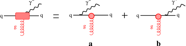
Figure 1: Born approximation for radiation of a photon by a quark in inelastic collision

Intuitively it is clear that if the electric charge gets no kick and is not accelerated, then no radiation happens.

This result is retained in the nonabelian case, namely a quark does not radiate gluons if the t-channel gluon provides no momentum transfer [6]. This is not a trivial result, since in this case a color current flows between the beam and target.

In the case of diffraction forward electromagnetic radiation vanishes as well, but this is less obvious. Indeed, even if the two-gluon exchange provides no momentum transfer, each of gluons can carry a transverse momentum. The relevant Born graphs for diffractive photon radiation are shown in Fig. 2.

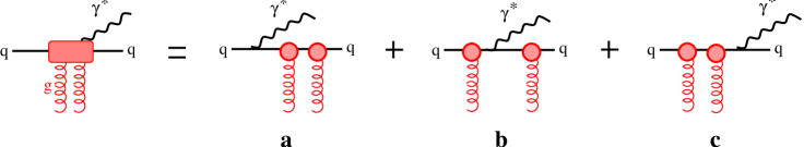
Figure 2: Born graphs for diffractive electromagnetic radiation by a quark.

Graph (b) does not contribute to radiation, provided that the radiation time considerably exceeds the duration time of interaction. Only graphs (a) and (c) can contribute, but they cause no radiation for forward scattering for the same reason as in the inelastic collision, Fig. 1.

This can be interpreted as a consequence of Landau-Pomeranchuk principle [7]: radiation depends on the whole strength of the kick, rather than on its structure, if the time scale of the kick is shorter than the radiation time. In other words, if two opposite kicks are separated by a short time interval, the radiation spectra from each of the two kicks interfere destructively and compensate each other [8, 9], i.e. no radiation occurs.

Notice that disappearance of abelian diffractive radiation in the forward direction goes along with the result of [10] that the diffractive cross section is proportional to the mean momentum transfer squared. That was, however, an oversimplified treatment of the Pomeron as a point-like vector meson.

Although a quark cannot radiate a dilepton in forward direction, a hadron can. That is possible due to transverse motion of the valence quarks in the hadron, i.e. abelian radiation even at a hard scale is sensitive to the hadron size, which is a dramatic break down of QCD factorization [11] (which has never been proven for this process). Failure of factorization for diffractive Drell-Yan reaction has been already known. It was found in [12, 13] that factorization fails due to the presence in the Pomeron of spectator partons. Below we demonstrate that factorization in Drell-Yan diffraction is even more broken due to presence of spectator partons in the colliding hadrons.

Notice that diffractive nonabelian (gluon) radiation is different, it does not vanish in the forward direction [5]. This is a direct manifestation of the nonabelian dynamics. In addition to the three graphs for electromagnetic radiation shown in Fig. 2, in the case of gluon radiation there is a fourth term corresponding to one of the t-channel gluons coupled to the radiated one. This term gives rise to a nonzero forward diffraction. This is confirmed by data, since a nonzero forward cross section of diffractive gluon radiation, called triple-Pomeron term in Regge approach, is well established experimentally [14]. Nevertheless, the cross section of diffractive gluon radiation turns out to be amazingly small. Indeed the Pomeron-proton total cross section extracted from data for large mass diffraction turns out to be only $2\,\mbox{mb}$, an order of magnitude smaller than for pion-proton. This effect is discussed and explained in Ref. [5].

2 Calculation of Feynman graphs

Although a quark cannot diffractively radiate photons in forward direction, a hadron can. Let us consider a $pp$ collision,

$$p_{b}+p_{t}\to\gamma^{*}+X+p_{t}\ ,$$ (2)

assuming that the initial beam nucleon and the final state consist of three valence quarks, $p_{b}={3q}_{i}$; $X={3q}_{f}$. The amplitude of the Drell-Yan (DY) reaction Eq. (2) has three terms,

$$A_{if}=A_{if}^{(1)}+A_{if}^{(2)}+A_{if}^{(3)}\ ,$$ (3)

where subscripts $i$ and $f$ correspond to initial and final states of the Drell-Yan diffractive reaction, Eq. (2).

Each term in (3) corresponds to radiation of the $\gamma^{*}$ by one of the valence quarks, and it includes contributions from tree graphs shown for $A_{if}^{(1)}$ in Fig. 3.

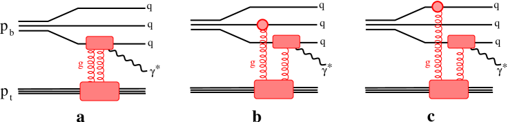
Figure 3: Born graphs for diffractive electromagnetic radiation by a proton

The first graph (a) leads to no radiation at $p_{T}=0$ as was explained above. The rest, graphs (b) and (c), can be calculated according to,

$$A_{if}^{(1)}(x_{\gamma},\vec{k})\Bigr{|}_{p_{T}=0}=\frac{i}{8\pi}\int d^{2}r_{1}d^{2}r_{2}d^{2}r_{3}d^{2}rdx_{q_{1}}dx_{q_{2}}dx_{q_{3}}$$ (4)

$$\times \Psi_{i}(\vec{r}_{1},\vec{r}_{2},\vec{r}_{3};x_{q_{1}},x_{q_{2}},x_{q_{3}})\Psi^{*}_{f}(\vec{r}_{1}+\alpha\vec{r},\vec{r}_{2},\vec{r}_{3};x_{q_{1}}-x_{\gamma},x_{q_{2}},x_{q_{3}})$$

$$\times \Sigma^{(1)}(\vec{r}_{1},\vec{r}_{2},\vec{r}_{3},\vec{r},\alpha)\,\Phi_{1}(\vec{r},\alpha)\,e^{-i\vec{k}\cdot\vec{r}}\ .$$

Here $\Psi_{i,f}$ are the light-cone wave functions of the $3q$ systems in the initial and final state respectively; $\vec{r}_{1},\ \vec{r}_{2}$ and $\vec{r}_{3}$ are the impact parameters of the quarks; $x_{q_{1}},x_{q_{2}},x_{q_{3}}$ are the fractions of the proton light-cone momentum carried by the quarks; $\vec{k}$ and $x_{\gamma}$ are the photon transverse and fractional longitudinal momenta; $\vec{r}$ is the transverse separation between the photon and the radiating quark; $\alpha=x_{\gamma}/x_{q_{1}}$; and $\Phi_{i}(\vec{r},\alpha)$ is the distribution amplitude for photon radiation by quark $q_{i}$ in the mixed representation, transverse coordinate and longitudinal momentum. The factor $\Sigma^{(1)}$ has the form,

$$\Sigma^{(1)}(\vec{r}_{1},\vec{r}_{2},\vec{r}_{3},\vec{r},\alpha)=\sigma(\vec{r}_{1}-\vec{r}_{2})-\sigma(\vec{r}_{1}-\vec{r}_{2}-\alpha\vec{r})+\sigma(\vec{r}_{1}-\vec{r}_{3})-\sigma(\vec{r}_{1}-\vec{r}_{3}-\alpha\vec{r})\ ,$$ (5)

where $\sigma(r_{T})$ is the universal dipole cross section [3].

The structure of this amplitude is easy to understand. According to the discussion in the previous section, the amplitude of diffractive radiation should be proportional to the difference between elastic amplitudes of the two Fock components, with and without the photon. In both cases only the 3-quark dipoles interact, but they have different sizes in the $|3q\rangle$ and $|3q\gamma^{*}\rangle$ components, therefore interact differently. Indeed, when a quark fluctuates into quark-photon with transverse separation $\vec{r}$, the final quark gets a transverse shift $\Delta\vec{r}=\alpha\vec{r}$, where $\alpha$ is the fraction of the quark momentum taken away by the photon. This shift is explicitly presented in (5).

For the model of symmetric proton wave function we use, the interference terms in the cross section cancel, since they are proportional to $Z_{1}Z_{2}+Z_{1}Z_{3}+Z_{2}Z_{3}=0$ (no cancellation occurs for neutrons), where $Z_{i}$ is the electric charge of the $i$th quark. Thus, summing over different final states $f$ one gets for the forward diffractive cross section,

$$\left.\frac{d\sigma_{sd}^{DY}}{dp_{T}^{2}}\right|_{p_{T}=0} = \frac{1}{64\pi}\sum\limits_{f}\int d^{2}k\,\frac{dx_{\gamma}}{x_{\gamma}}\sum\limits_{n=1}^{3}\left|A^{(n)}_{if}\right|^{2}$$ (6)

$$= \frac{1}{64\pi}\sum\limits_{f}\int d^{2}k\,\frac{dx_{\gamma}}{x_{\gamma}}\,\left|A^{(1)}_{if}\right|^{2}\left(1+\frac{Z_{2}^{2}}{Z_{1}^{2}}+\frac{Z_{3}^{2}}{Z_{1}^{2}}\right)\ .$$

Employing completeness,

$$\sum\limits_{f}\Psi_{f}(\vec{r}_{1},\vec{r}_{2},\vec{r}_{3};x_{q_{1}},x_{q_{2}},x_{q_{3}})\Psi^{*}_{f}(\vec{r}_{1}^{\,\prime},\vec{r}_{2}^{\,\prime},\vec{r}_{3}^{\,\prime};x_{q_{1}}^{\prime},x_{q_{2}}^{\prime},x_{q_{3}}^{\prime})$$ (7)

$$= \prod\limits_{j=1}^{3}\delta(\vec{r}_{j}-\vec{r}_{j}^{\,\prime})\delta(x_{q_{j}}-x_{q_{j}}^{\prime})\,$$

we arrive at

$$\left.\frac{d\sigma_{sd}^{DY}}{dp_{T}^{2}}\right|_{p_{T}=0} = \frac{\sum Z_{q}^{2}}{64\pi}\int d^{2}r_{1}d^{2}r_{2}d^{2}r_{3}d^{2}r\,dx_{q_{1}}dx_{q_{2}}dx_{q_{3}}\,\frac{dx_{\gamma}}{x_{\gamma}}\,\left|\tilde{\Phi}(\vec{r},\alpha)\right|^{2}$$ (8)

$$\times \left|\Psi_{i}(\vec{r}_{1},\vec{r}_{2},\vec{r}_{3};x_{q_{1}},x_{q_{2}},x_{q_{3}})\right|^{2}\left|\Sigma^{(1)}(\vec{r}_{1},\vec{r}_{2},\vec{r}_{3},\vec{r},\alpha)\right|^{2}\ .$$

Here $\tilde{\Phi}(\vec{r},\alpha)=\Phi_{i}(\vec{r},\alpha)/Z_{i}$ is the amplitude of photon radiation by a quark with charge one.

To progress further we assume the Gaussian shape for the quark distribution in the proton,

$$\left|\Psi_{i}(\vec{r}_{1},\vec{r}_{2},\vec{r}_{3};x_{q_{1}},x_{q_{2}},x_{q_{3}})\right|^{2} = \frac{3a^{2}}{\pi^{2}}\,\exp[-a(r_{1}^{2}+r_{2}^{2}+r_{3}^{2})]\rho(x_{q_{1}},x_{q_{2}},x_{q_{3}})$$ (9)

$$\times \delta(\vec{r}_{1}+\vec{r}_{2}+\vec{r}_{3})\,\delta(1-x_{q_{1}}-x_{q_{2}}-x_{q_{3}})\ ,$$

where $a=\langle r_{ch}^{2}\rangle^{-1}$ is the inverse proton mean charge radius squared. The three-body distribution function $\rho(x_{q_{1}},x_{q_{2}},x_{q_{3}})$ should reproduce the valence quark distribution in the proton,

$$\int dx_{q_{2}}dx_{q_{3}}\,\rho(x_{q_{1}},x_{q_{2}},x_{q_{3}})=\rho_{q_{1}}(x_{q_{1}})\ .$$ (10)

Summing different quark and antiquark species one arrives at the proton structure function [15],

$$\sum\limits_{q}Z_{q}^{2}\,\left[\rho_{q}(x)+\rho_{\bar{q}}(x)\right]={1\over x}\,F_{2}(x)\ .$$ (11)

At this point we generalize our three-body quark wave function (9) to a multi-body one including antiquarks. However, we keep the same simple coordinate part of the wave function.

In what follows we rely on the popular saturated form of the dipole cross section,

$$\sigma(r)=\sigma_{0}\left(1-e^{-r^{2}/R_{0}^{2}}\right)\,$$ (12)

where the parameters fitted to DIS data at small $x$ can be found in [16].

The distribution functions have the form,

$$\tilde{\Phi}^{L}(\vec{r},\alpha)=\frac{\sqrt{\alpha_{em}}}{\pi}\,M(1-\alpha)\,\chi^{\dagger}_{f}\,\chi_{i}\,K_{0}(\tau r)\ ;$$ (13)

$$\tilde{\Phi}^{T}(\vec{r},\alpha) = \frac{\sqrt{\alpha_{em}}}{2\pi}\,\chi^{\dagger}_{f}\,\left\{i\alpha^{2}m_{q}[\vec{\sigma}\times\vec{e}]\cdot\vec{n}-i(2-\alpha)\,\vec{e}\cdot\vec{\nabla}\right.$$ (14)

$$- \left.\alpha[\vec{\sigma}\times\vec{e}]\cdot\vec{\nabla}\right\}\chi_{i}\,K_{0}(\tau r)\ ,$$

for radiation of longitudinally and transversely polarized photons respectively. Here $K_{0}(\tau r)$ is the modified Bessel function;

$$\tau^{2}=M^{2}(1-\alpha)+m_{q}^{2}\,\alpha^{2}\ ;$$ (15)

$\chi_{i,f}$ are the spinors assigned to the quark before and after the radiation respectively; $\vec{\sigma}$ is the Pauli matrix; $\vec{n}$ is a unit vector directed along the initial collision momentum; $m_{q}$ is the quark mass.

Now we are in a position to perform integration over coordinates in (8). Using the integral representation for the modified Bessel function,

$$K_{0}(\tau r) = {1\over 2}\int\limits_{0}^{\infty}\frac{dt}{t}\,\exp\left(-\frac{\tau^{2}r^{2}}{4t}\right)\ ;$$

$$K_{0}^{2}(\tau r) = {1\over 4}\int\limits_{0}^{\infty}\frac{dt}{t}\int\limits_{0}^{\infty}\frac{du}{u}\,\exp\left[-\left(\frac{\tau^{2}r^{2}}{4t}+1\right)(t+u)\right]\ ,$$ (16)

we arrive at the longitudinal cross section of diffractive DY reaction,

$$\left.\frac{d\sigma_{sd}^{DY(L)}}{dM^{2}\,dx_{1}\,dp_{T}^{2}}\right|_{p_{T}=0} = \frac{\sigma_{0}^{2}}{x_{1}}\,\frac{2\alpha^{2}_{em}}{3(8\pi)^{3}}\int\limits_{x_{1}}^{1}d\alpha\,\frac{(1-\alpha)^{2}}{\alpha}\,F_{2}(x_{1}/\alpha)\int\limits_{0}^{\infty}du\,e^{-u}$$ (17)

$$\times \frac{1}{\tau^{2}}\,\left[\frac{1+2w_{1}-4w_{2}}{1+4z}+\frac{1+2w_{3}-4w_{4}}{(1+3z)(1+z)}\right].$$

The cross section of radiation of transversely polarized dileptons summed over polarizations reads

$$\left.\frac{d\sigma_{sd}^{DY(T)}}{dM^{2}\,dx_{1}\,dp_{T}^{2}}\right|_{p_{T}=0}=\frac{\sigma_{0}^{2}}{M^{2}\,x_{1}}\,\frac{\alpha^{2}_{em}}{3(8\pi)^{3}}\int\limits_{x_{1}}^{1}\frac{d\alpha}{\alpha}\,F_{2}(x_{1}/\alpha)\int\limits_{0}^{\infty}du\,e^{-u}$$ (18)

$$\times \left\{\alpha^{4}\frac{m_{q}^{2}}{\tau^{2}}\,\left[\frac{1+2w_{1}-4w_{2}}{1+4z}+\frac{1+2w_{3}-4w_{4}}{(1+3z)(1+z)}\right]\right.$$

$$+ \left.\frac{1-\alpha+\alpha^{2}}{u}\left[\frac{2+o_{1}-2o_{2}}{1+4z}+\frac{2+o_{3}-2o_{4}}{(1+3z)(1+z)}\right]\right\}$$

Here $x_{1}\equiv x_{\gamma}$ and $x_{2}$ are the standard DY variables,

$$x_{1}=\frac{2qP_{1}}{s}\ ;\hskip 56.9055ptx_{2}=\frac{2qP_{2}}{s}\ ,$$ (19)

where $q$ and $P_{1,2}$ are the 4-momenta of the radiated dilepton, and projectile/target protons respectively. Other notations in (18) are,
$\displaystyle z$ $\displaystyle=$ $\displaystyle\frac{\langle r_{ch}^{2}\rangle}{R_{0}^{2}}\ ;$ $\displaystyle w_{i}$ $\displaystyle=$ $\displaystyle\frac{1-v_{i}^{2}}{4v_{i}}\,\ln\left(\frac{1+v_{i}}{1-v_{i}}\right)\ ;$ $\displaystyle\lambda_{1}^{2}$ $\displaystyle=$ $\displaystyle\frac{8}{R_{0}^{2}(1+4z)}\ ;$ $\displaystyle\lambda_{3}^{2}$ $\displaystyle=$ $\displaystyle\frac{8}{R_{0}^{2}(1+3z)}\ ;$       $\displaystyle o_{i}$ $\displaystyle=$ $\displaystyle(1-v_{i}^{2})(2w_{i}+1)\ ;$ $\displaystyle v_{i}$ $\displaystyle=$ $\displaystyle\sqrt{\frac{u\,\lambda_{i}^{2}/\tau^{2}}{4+u\,\lambda_{i}^{2}/\tau^{2}}}\ ;$ $\displaystyle\lambda_{2}^{2}$ $\displaystyle=$ $\displaystyle\frac{4(1+2z)}{R_{0}^{2}(1+4z)}\ ;$ (20) $\displaystyle\lambda_{4}^{2}$ $\displaystyle=$ $\displaystyle\frac{4(1+2z)}{R_{0}^{2}(1+3z)(1+z)}\ ;$
and $i=1,2,3,4$.

Since the forward cross section is known, the total diffractive cross section can be estimated as,

$$\frac{d\sigma^{DY}_{sd}}{dx_{1}}=\frac{1}{B^{DY}_{sd}(s)}\,\left.\frac{d\sigma^{DY}_{sd}}{dx_{1}\,dp_{T}^{2}}\right|_{p_{T}=0}\ ,$$ (21)

where $B^{DY}_{sd}(s)$ is the slope of the $t$-dependence of the cross section, which is similar to the corresponding slope measured in diffractive DIS.

3 Unitarity corrections

While the radiated leptons do not interact with the target, the accompanying quarks do, and they can easily initiate an inelastic interaction followed by multiparticle production filling up the rapidity gap. Therefore, the survival probability of the gap causes a suppression for the diffractive cross section. This is easy to take into account in the impact parameter representation. The amplitude Eq. (3) acquires a factor,

$$A_{if}(b)\Rightarrow A_{if}(b)\,\left[1-{\rm Im}f^{pp}_{el}(b)\right]\ ,$$ (22)

where $f^{pp}_{el}(b)$ is the partial elastic amplitude. After squaring this amplitude and integration over impact parameter we arrive at the cross section which is different from one in Eq. (21) by a suppression factor $K$, $d\sigma^{DY}_{sd}/dx_{1}\Rightarrow K\,d\sigma^{DY}_{sd}/dx_{1}$, where [17]

$$K=\left\{1-{1\over{\pi}}\,\frac{\sigma^{pp}_{tot}(s)}{B^{DY}_{sd}(s)+2B^{pp}_{el}(s)}+\frac{1}{(4\pi)^{2}}\,\frac{\left[\sigma^{pp}_{tot}(s)\right]^{2}}{B^{pp}_{el}(s)\left[B^{DY}_{sd}(s)+B^{pp}_{el}(s)\right]}\right\}\ .$$ (23)

Here the elastic slope depends on energy as $B^{pp}_{el}(s)=B^{0}_{el}+2\,\alpha^{\prime}_{{\bf I\!P}}\,\ln(s/s_{0})$ with $B^{0}_{el}=7.5\,\mbox{GeV}^{-2}$, $s_{0}=1\,\mbox{GeV}^{2}$. The slope of single-diffractive DY cross section can be estimated as, $B^{DY}_{sd}(s)\approx\langle r_{ch}^{2}\rangle/3+2\,\alpha^{\prime}_{{\bf I\!P}}\,\ln(s/s_{0})$, where the proton mean charge radius squared $\langle r_{ch}^{2}\rangle=0.8\,\mbox{fm}^{2}$.

Notice that this eikonal expression for the gap survival probability is a conservative estimate. Inclusion of corrections related to intermediate diffractive excitations of the beam particle (so called Gribov corrections [18]) make the medium more transparent, i.e. increase the survival probability of the rapidity gap [17].

Our estimate Eq. (23) can be compared with the results of more elaborate models [19, 20, 21, 22] incorporating a part of the Gribov corrections. The predicted suppression factors have similar orders of magnitude. Notice that one can easily replace the suppression factor (23) by a preferable one.

4 Diffractive vs Inclusive

We should compare the diffractive DY cross section with the inclusive one, which also can be calculated within the dipole approach [23, 24, 15],

$$\frac{d\sigma_{inc}^{DY(L,T)}}{dx_{1}\,dM^{2}}=\frac{1}{M^{2}\,x_{1}}\,\frac{\alpha_{em}^{2}}{3\pi}\int\limits_{x_{1}}^{1}\frac{d\alpha}{\alpha}\,F_{2}(x_{1}/\alpha)\int d^{2}r\,\left|\tilde{\Phi}^{L,T}(\vec{r},\alpha)\right|^{2}\,\sigma\left(\alpha r,x_{2}\right)$$ (24)

This simple formula reproduces with high precision the cross section measured by E772 [25] and E866 [26] experiments at Fermilab, and agrees quite well with the results obtained from much more complicated NLO parton model calculations [27].

Applying Eqs. (12)-(16) to Eq. (24) we get,

$$\frac{d\sigma_{inc}^{DY(L)}}{dx_{1}\,dM^{2}}=\frac{\sigma_{0}}{x_{1}}\,\frac{\alpha^{2}_{em}}{24\pi^{2}}\int\limits_{x_{1}}^{1}d\alpha\,\frac{(1-\alpha)^{2}}{\alpha}\,F_{2}(x_{1}/\alpha)\int\limits_{0}^{\infty}du\,e^{-u}\,\frac{1-2w}{\tau^{2}}\ ;$$ (25)

$$\frac{d\sigma_{inc}^{DY(T)}}{dx_{1}\,dM^{2}} = \frac{\sigma_{0}}{x_{1}\,M^{2}}\,\frac{\alpha^{2}_{em}}{48\pi^{2}}\int\limits_{x_{1}}^{1}\frac{d\alpha}{\alpha}\,F_{2}(x_{1}/\alpha)\int\limits_{0}^{\infty}du\,e^{-u}\,$$ (26)

$$\times \left[\frac{\alpha^{4}\,m_{q}^{2}}{\tau^{2}}\,(1-2w)+\frac{1-\alpha+\alpha^{2}}{u}\,(2-o)\right]\ .$$

The notations here are similar to (20),
$\displaystyle o$ $\displaystyle=$ $\displaystyle(1-v^{2})(2w+1)\ ;$ $\displaystyle v$ $\displaystyle=$ $\displaystyle\sqrt{\frac{u\,\lambda^{2}/\tau^{2}}{4+u\,\lambda^{2}/\tau^{2}}}\ ;$ $\displaystyle w$ $\displaystyle=$ $\displaystyle\frac{1-v^{2}}{4v}\,\ln\left(\frac{1+v}{1-v}\right)\ ;$ $\displaystyle\lambda^{2}$ $\displaystyle=$ $\displaystyle\frac{4}{R_{0}^{2}}\ ;$ (27)

We perform our calculations with the proton structure function parametrized as,

$$F_{2}(x,Q^{2})=A(x)\left[\frac{\ln(Q^{2}/\Lambda^{2})}{\ln(Q_{0}^{2}/\Lambda^{2})}\right]^{B(x)}\left[1+\frac{C(x)}{Q^{2}}\right]\ ,$$ (28)

with $Q_{0}^{2}=20\,\mbox{GeV}^{2}$ and $\Lambda=0.25\,\mbox{GeV}$. This parametrization was fitted to available data for $F_{2}(x,Q^{2})$ from different experiments. The form and fitted parameters for the functions $A(x),\ B(x)$ and $C(x)$ can be found in the Appendix of [28].

For the parameters of the dipole cross section, Eq. (12), we use the results of the fit of Ref. [16] to HERA data: $\sigma_{0}=23.03\,\mbox{fm}$; $R_{0}(x_{2})=0.4\,\mbox{fm}\times(x_{2}/x_{0})^{0.144}$, where $x_{0}=3.04\times 10^{-4}$.

We calculated the ratio of the diffractive to inclusive cross sections. The results are plotted in Fig. 4 as function of the dilepton effective mass squared at fixed $x_{1}=0.5,\ 0.9$ and energies $\sqrt{s}=40\,\mbox{GeV},\ 500\,\mbox{GeV}$ and $14\,\mbox{TeV}$.

Figure 4: Ratio of diffractive to inclusive DY cross sections as function of $M^{2}$ at fixed $x_{1}=0.5$ (solid curves) and $x_{1}=0.9$ (dashed) and energies (from top to bottom) $\sqrt{s}=40\,\mbox{GeV},\ 500\,\mbox{GeV}$ and $14\,\mbox{TeV}$.

In these calculations we summed the contributions of longitudinal and transverse parts both in the diffractive and inclusive cross sections.

The results depicted in Fig. 4 demonstrate unusual effects. The diffractive-to-inclusive cross section ratio is steeply falling with energy. This is counterintuitive, since diffraction, which is proportional to the dipole cross section squared, should rise with energy steeper than the total inclusive cross section. At the same time, the ratio rises with the hard scale, $M^{2}$. This also looks strange, since diffraction is usually associated with soft interactions [29].

To understand these remarkable features of DY diffraction we should return back to the original diffractive amplitude, Eq. (4)-(5). As we emphasized, the diffractive amplitude is given by the difference between the cross sections of the relevant Fock states with and without the dilepton. This is explicitly incorporated into Eq. (5). Assuming $r\sim 1/M\ll R_{0}(x_{2})$ we can expand this cross section difference as,

$$\sigma(\vec{R})-\sigma(\vec{R}-\alpha\vec{r})=\frac{2\alpha\,\sigma_{0}}{R_{0}^{2}(x_{2})}\,e^{-R^{2}/R_{0}^{2}(x_{2})}\,\left(\vec{r}\cdot\vec{R}\right)+O(r^{2})\ .$$ (29)

This is an interesting result: the amplitude is linear in $r$, i.e. the diffractive cross section is quadratic function of $r$. This is different from diffraction in DIS where the cross section is $\propto r^{4}$. The latter is predominantly a soft process, since the end-point $\bar{q}q$ fluctuations, $\alpha\to 0,\ 1$, have no scale dependence, only their weight is $\propto 1/Q^{2}$. Therefore these soft fluctuations dominate the diffractive DIS cross section [29, 30]. However, since diffractive DY cross section is $\propto r^{2}$, soft and hard interactions contribute on the same footing, and their interplay does not depend on the scale, similar to inclusive DY or DIS.

Moreover, expression (30) leads in Eq. (8) to the same integral over $r$ and $\alpha$ as in the inclusive cross section Eq. (24). Therefore, all energy and scale dependence of the diffractive-to-inclusive cross section ratio comes via the $x_{2}$-dependent factor,

$$\frac{\sigma^{DY}_{sd}}{\sigma^{DY}_{inc}}\ \propto\ \frac{1}{R_{0}^{2}(x_{2})}\,e^{-2R^{2}/R_{0}^{2}(x_{2})}\ .$$ (30)

Since for light hadrons $R_{0}^{2}(x_{2})<2R^{2}$, this expression rises with $R_{0}$, i.e. with $x_{2}=M^{2}/x_{1}s$. This explains why the ratio depicted in Fig. 4 falls down with energy, but rises with $M^{2}$. Note that the falling energy dependence is partially due to the absorptive corrections (23).

We found that both the diffractive and inclusive DY cross sections are dominated by radiation of transversely polarized DY pairs. This is demonstrated in Fig. 5 where we plotted the ratios of the longitudinal to transverse cross sections for inclusive diffractive DY reaction as function of $M^{2}$ at different energies.

Figure 5: Ratio of longitudinal to transverse parts of diffractive DY cross sections as function of $M^{2}$ at fixed $x_{1}=0.5$. The predictions are made for energies, $\sqrt{s}=40\,\mbox{GeV}$ (dotted), $\sqrt{s}=500\,\mbox{GeV}$ (dashed), and $\sqrt{s}=14\,\mbox{TeV}$ (solid).

These ratios turn out to be very similar to that for inclusive DY processes.

We see that the diffractive ratios are close to the inclusive ones. They do not exhibit any strong dependence on energy, but fall down at harder scales, similar to DIS [31]. This fall is related to the suppression of the end-point, $\alpha\to 1$, of longitudinally polarized DY fluctuations in equation(13).

5 Summary

Contrary to the simple intuition based on QCD factorization, diffractive DY processes have properties quite different from what is known about DIS and nonabelian radiation.

• A quark cannot radiate noninteracting particles (photons, dileptons, gauge bosons, Higgs, etc.) diffractively in the forward direction, i.e. without gaining any momentum transfer. This is a manifestation of the general principle: if a charge is accelerated and then immediately decelerated, these two sources of radiation interfere destructively and cancel each other [8, 9]. This can also be interpreted in terms of the Landau-Pomeranchuk principle: radiation at times longer than the time interval of the interaction depends only on the strength of the whole kick, but does not resolve its structure (a single or multiple kicks).

  The nonabelian case, QCD, is different: a quark can radiate gluons diffractively in the forward direction. This happens due to possibility of interaction between the radiated gluon and the target.

• Nevertheless, a hadron can radiate abelian fields diffractively and in the forward direction. This process involves the spectator quarks as is illustrated in Fig. 3, and for this reason the cross section depends on the hadronic size and rises with it. This is an apparent and strong breakdown of factorization.

  The situation in the nonabelian case is different. The main contribution to the cross section comes from diffractive gluon radiation by a single quark. Interaction with the spectator quarks has little impact and vanishes at large separations.

• The ratio of the cross section of diffractive radiation of abelian fields to the inclusive one is steeply falling with energy as depicted in Fig. 4. This occurs even without unitarity corrections which make the fall even steeper, and is a result of the saturated shape of the dipole cross section. If this cross section was rising like $\sigma(r)\propto r^{2}$, the ratio would be energy independent (up to unitarity corrections). This property is strikingly opposite to what would follow from factorization [11].

  This again is different in the nonabelian case, since here without unitarity corrections the diffractive cross section rises faster than the inclusive one. This happens because the diffraction cross section is a quadratic function of the dipole cross section, while the inclusive is linear .

  This is also different from DIS where the diffraction to inclusive ratio rises with energy.

• Unexpectedly, the fraction of diffractive events to the total inclusive cross section of abelian radiation rises with the dilepton effective mass $M$ (see Fig. 4). This effect has the same origin as the energy dependence, the dipole cross section which levels off at large separations. On the contrary, the fraction of diffraction in the total DIS cross section is slowly, logarithmically, falling with the hard scale. Same would be true for Drell-Yan diffraction if factorization were correct.

  The rise of diffraction with the hard scale looks counterintuitive, since diffraction is usually associated with soft interactions. However, that is not true for diffractive DY processes.

• Hard and soft interactions contribute to DY diffraction on the same footing, and their ratio is scale independent like in inclusive DY process. This is a result of the specific property of DY diffraction: its cross section is a linear, rather than quadratic function of the dipole cross section.

  On the contrary, diffractive DIS is predominantly a soft process, because its cross section is proportional to $\sigma^{2}(r)$

• The main features of our results for Drell-Yan reaction are valid for other diffractive abelian processes, like production of direct photons, Higgsstrahlung, radiation of $Z$ and $W$ bosons. One should not rely on QCD factorization for these reactions.

• Measurement of diffractive DY processes in a wide energy range from fixed target experiments up to the modern colliders, RHIC, Tevatron and LHC, would provide a precious direct probe for the behavior of the dipole cross section at large distances, above the saturated radius, $r>R_{0}$.

Acknowledgments: We are grateful to Hans-Jürgen Pirner for useful discussions. A.V.T. thanks the Physics Department of the University Federico Santa Maria for the hospitality. This work is supported in part by Fondecyt (Chile) grants, numbers 1030355, 1050519, 1050589 and 7050175, and by DFG (Germany) grant PI182/3-1.

References

- [1] E. Feinberg and I.Ya. Pomeranchuk, Nuovo. Cimento. Suppl. 3 (1956) 652.
- [2] M.L. Good and W.D. Walker, Phys. Rev. 120, 1857 (1960).
- [3] B.Z. Kopeliovich, L.I. Lapidus and A.B. Zamolodchikov, Sov. Phys. JETP Lett. 33 (1981) 595; Pisma v Zh. Exper. Teor. Fiz. 33, 612 (1981).
- [4] G. Bertsch, S.J. Brodsky, A.S. Goldhaber and J.F. Gunion, Phys. Rev. Lett. 47, 297 (1981).
- [5] B.Z. Kopeliovich, A. Schäfer and A.V. Tarasov, Phys. Rev. D62, 054022 (2000).
- [6] J.F. Gunion and G. Bertsch, Phys. Rev. D25, 746 (1982).
- [7] L.D. Landau, I.Ya. Pomeranchuk, ZhETF, 505 (1953); Doklady AN SSSR 92, 535, 735 (1953).
- [8] B.Z. Kopeliovich and A.B. Zamolodchikov, Multiple color-exchange scattering of high-energy hadrons in nuclei: Proc. of the VI Balaton Conf. on Nucl. Phys., p. 73, Balatonfüred, Hungary, 1983.
- [9] F. Niedermayer, Phys. Rev. D34, 3494 (1986).
- [10] S.M. Berman, D.J. Levy and T.L. Neff, Phys. Rev. Lett. 23, 1363 (1969).
- [11] A. Donnachie and P.V. Landshoff, Nucl. Phys. B303, 634 (1988).
- [12] J.C. Collins, L. Frankfurt, M. Strikman, Phys.Lett. B307, 161 (1993).
- [13] J.C. Collins, Phys.Rev. D57, 3051 (1998).
- [14] Yu.M. Kazarinov, B.Z. Kopeliovich, L.I. Lapidus and I.K. Potashnikova, JETP 70 (1976) 1152.
- [15] B.Z. Kopeliovich, J. Raufeisen and A.V. Tarasov, Phys. Lett. B503, 91 (2001).
- [16] K. Golec-Biernat and M. Wüsthoff, Phys. Rev. D 59 (1999) 014017.
- [17] B.Z. Kopeliovich, I.K. Potashnikova, Ivan Schmidt, Phys. Rev. C73, 034901 (2006).
- [18] V.N. Gribov, Sov. Phys. JETP 56, 892 (1968).
- [19] E. Gotsman, E.M. Levin, and U. Maor, Z. Phys. C57, 677 (1993); Phys. Rev. D49, 4321 (1994); Phys. Lett. B353, 526 (1995); Phys. Lett. B347, 424 (1995).
- [20] E. Gotsman et al., arXiv: hep-ph/0511060.
- [21] V.A. Khoze, A.D. Martin, and M.G. Ryskin, Eur. Phys. J. C14, 525 (2000);
- [22] A.B. Kaidalov, V.A. Khoze, A.D. Martin, and M.G. Ryskin, Eur. Phys. J. C33, 261 (2004).
- [23] B. Z. Kopeliovich, proc. of the workshop Hirschegg ’95: Dynamical Properties of Hadrons in Nuclear Matter, Hirschegg January 16-21, 1995, ed. by H. Feldmeyer and W. Nörenberg, Darmstadt, 1995, p. 102 (hep-ph/9609385).
- [24] B.Z. Kopeliovich, A. Schaefer and A.V. Tarasov, Phys. Rev. C59 (1999) 1609
- [25] E772 Collaboration, P.L. McGaughey et al., Phys.Rev. D50, 3038 (1994); [Erratum-ibid, D60, 119903 (1994).
- [26] E866 Collaboration, J.C. Webb et al., hep-ex/0302019, to appear in Phys. Rev. Lett.
- [27] J. Raufeisen, J.C. Peng and G.C. Nayak, Phys. Rev. D 66, 034024 (2002).
- [28] SMC Collaboration, B. Adeva et al., Phys. Rev. D58, 112001 (1998).
- [29] B.Z. Kopeliovich and B. Povh, Z. Phys. A356, 467 (1997).
- [30] B.Z. Kopeliovich, I.K. Potashnikova and I. Schmidt, Diffraction in QCD, lecture given, at ILAHEP, Porto Alegre, 2005 (hep-ph/0604097).
- [31] B.Z. Kopeliovich, J. Raufeisen and A.V. Tarasov, Phys. Rev. C62, 035204 (2000).