Dynamical breakdown of Abelian gauge chiral symmetry by strong Yukawa interactions

Abstract

We consider a model with anomaly-free Abelian gauge axial-vector symmetry, which is intended to mimic the standard electroweak gauge chiral $SU(2)_{L}\times U(1)_{Y}$ theory. Within this model we demonstrate: (1) Strong Yukawa interactions between massless fermion fields and a massive scalar field carrying the axial charge generate dynamically the fermion and boson proper self-energies, which are ultraviolet-finite and chirally noninvariant. (2) Solutions of the underlying Schwinger-Dyson equations found numerically exhibit a huge amplification of the fermion mass ratios as a response to mild changes of the ratios of the Yukawa couplings. (3) The ‘would-be’ Nambu-Goldstone boson is a composite of both the fermion and scalar fields, and it gives rise to the mass of the axial-vector gauge boson. (4) Spontaneous breakdown of the gauge symmetry further manifests by mass splitting of the complex scalar and by new symmetry-breaking vertices, generated at one loop. In particular, we work out in detail the cubic vertex of the Abelian gauge boson.

I Introduction

Use of the general principle of spontaneous breakdown of continuous symmetry for the $SU(2)_{L}\times U(1)_{Y}$ invariant field theory description of electroweak phenomena is a necessity. Hard symmetry-breaking mass terms of both gauge and fermion fields ruin, either directly or by virtue of the loops, decent high-energy behavior of certain scattering amplitudes.

In this respect the standard ‘Higgs’ realization of spontaneous breakdown of the electroweak symmetry deserves admiration. At the expense of introducing a sector with a condensing scalar doublet it defines the operational (renormalizable, weakly coupled) description of virtually all electroweak phenomena so far explored.

Because of theoretical drawbacks of the Higgs mechanism there are alternatives and/or generalizations thereof Eidelman et al. (2004) (and references therein). In the near future the Large Hadron Collider at CERN will harshly test all of them. The aim of this paper is to add to the already existing list yet another realization of spontaneous breakdown of chiral and gauge symmetry. For clarity we illustrate it on physically and technically transparent Abelian prototype. Comparison with the standard Abelian Higgs mechanism can easily be made at any stage by heart.

The basic idea Brauner and Hošek (2005) is simple but subtle: As in the standard Higgs realization we employ the complex scalar field but with an ordinary mass term of a complex scalar. Hence, in accordance with common wisdom there will be no spontaneous symmetry breakdown in the scalar sector itself. Subtle is the nonperturbative self-consistence: The chiral symmetry breaking fermion proper self-energy is both caused and causes the symmetry-breaking scalar proper self-energy, both solely due to a strong Yukawa interaction.

The subsequent question of whether a massless gauge field introduced by gauging the $U(1)$ axial symmetry describes a massless or a massive spin-1 particle is dynamical and it was in general answered by Schwinger Schwinger (1962): If, within a given dynamics, the gauge field polarization tensor develops a massless pole, its residue approximates the gauge boson mass squared Jackiw and Johnson (1973). Both in the Abelian Higgs model and in the model presented below the massless pole in the gauge field polarization tensor is due to the ‘would-be’ Nambu-Goldstone (NG) boson of the underlying global symmetry. While in the Higgs mechanism the NG boson is pre-prepared in the elementary scalar field, in our case it is a composite object of both the fermion and the scalar fields.

Finally, it is easy to realize that due to the dynamical generation of the symmetry-breaking pieces in fermion and scalar field propagators there are new effective symmetry-breaking vertices between the mass eigenstates of the fields.

The paper is organised as follows: After introducing the model by its Lagrangian we discuss the possibility of the dynamical spontaneous breaking of the chiral symmetry and introduce the appropriate formalism. Then we explore the consequences of the global symmetry: the existence of the ‘would-be’ NG boson and its interaction vertices with other particles. In this part we only repeat the main results of our preceding paper Brauner and Hošek (2005) so we do not go into a detail. After this we present some consequences of the local symmetry: the mass of the gauge boson, induced by the bilinear coupling with the ‘would-be’ NG boson, and the existence of the effective trilinear coupling of the gauge bosons. In the end we present our numerical results, especially the possibility of an arbitrarily high ratio of fermion masses with Yukawa coupling constants being of the same order of magnitude, together with the description of our numerical procedure.

II The Model

In the full generality the model is defined by the Lagrangian

$$\mathcal{L} = \bar{\psi}_{1}\mathrm{i}\not{\mathrm{D}}\psi_{1}+\bar{\psi}_{2}\mathrm{i}\not{\mathrm{D}}\psi_{2}+(\mathrm{D}_{\mu}\phi)^{\dagger}(\mathrm{D}^{\mu}\phi)$$

$${}-M^{2}\phi^{\dagger}\phi-\frac{1}{2}\lambda(\phi^{\dagger}\phi)^{2}-\frac{1}{4}F_{\mu\nu}F^{\mu\nu}$$

$${}+\mathcal{L}_{\rm{Yukawa}}\,,$$

where the Yukawa interaction Lagrangian reads

$$\begin{split}\mathcal{L}_{\rm{Yukawa}}&\>=\>\hphantom{+\,}y_{1}(\bar{\psi}_{1L}\psi_{1R}\phi+\bar{\psi}_{1R}\psi_{1L}\phi^{\dagger})\\ &\hphantom{\>=\>}\,+\,y_{2}(\bar{\psi}_{2R}\psi_{2L}\phi+\bar{\psi}_{2L}\psi_{2R}\phi^{\dagger})\,.\end{split}$$ (2)

The Lagrangian possesses various symmetries. First, it is invariant under the global $U(1)_{V_{1}}\times U(1)_{V_{2}}\times U(1)_{A}$ symmetry. The two global vector $U(1)$ symmetries are generated by the fermion number operators of the fermions 1 and 2 and represent separate conservation of the number of both fermion species. The two naive independent axial $U(1)$ transformations of the fermions 1 and 2 are related to each other by the Yukawa couplings to the scalar field $\phi$. Second, the Lagrangian is invariant under the local (gauge) $U(1)_{A}$ transformations, acting on the fields as

$$\psi_{j} \rightarrow \mathrm{e}^{\mathrm{i}\theta(x)Q_{j}\gamma_{5}}\psi_{j}\,,$$

$$\phi \rightarrow \mathrm{e}^{-2\mathrm{i}\theta(x)}\phi\,,$$ (3)

$$A_{\mu} \rightarrow A_{\mu}+\frac{1}{g}\partial_{\mu}\theta(x)\,,$$

where the axial charges $Q_{1}$, $Q_{2}$ are defined as

$$\begin{split}Q_{1}&\>=\>+1\,,\\ Q_{2}&\>=\>-1\,.\end{split}$$ (4)

Considering two fermion species with opposite axial charges provides the simplest solution to an important theoretical constraint imposed on the model, which is the absence of the axial anomaly. The Yukawa coupling constants $y_{1}$, $y_{2}$ are arbitrary real numbers. For the sake of simplicity we do not consider a more general Yukawa Lagrangian, allowing them to be complex.

III Global Symmetry

III.1 Self-energies & masses

In the first step we switch off the gauge interaction $(g=0)$ and demonstrate the spontaneous breakdown of the global $U(1)_{A}$ symmetry by finding symmetry-breaking proper self-energies in the fermion and scalar field propagators. We follow the general self-consistent nonperturbative method suggested by Nambu (and Jona-Lasinio) Nambu (1960); Nambu and Jona-Lasinio (1961).

First of all, it is convenient to introduce the Nambu-like doublet field for the scalar

$$\Phi=\left(\begin{array}[]{c}\phi\\ \phi^{\dagger}\end{array}\right)$$ (5)

and its matrix propagator

$$\begin{split}\mathrm{i}D(x-y)&=\langle 0|T\{\Phi(x)\Phi^{\dagger}(y)\}|0\rangle\\ &=\left(\begin{array}[]{cc}\langle\phi\phi^{\dagger}\rangle&\langle\phi\phi\rangle\\ \langle\phi^{\dagger}\phi^{\dagger}\rangle&\langle\phi^{\dagger}\phi\rangle\end{array}\right)\,.\end{split}$$ (6)

The point is that this formalism allows us to treat the symmetry-preserving (the diagonal entries) as well as the symmetry-breaking (the off-diagonal entries) scalar propagators on the same footing. Similarly in the fermion sector, it is convenient to deal with the propagator

$$\mathrm{i}S(x-y)=\langle 0|T\{\psi(x)\bar{\psi}(y)\}|0\rangle\,,$$ (7)

as it also contains both the symmetry-preserving (e.g. $\langle\psi_{L}\bar{\psi}_{L}\rangle$) and the symmetry-breaking (e.g. $\langle\psi_{L}\bar{\psi}_{R}\rangle$) fermion propagators.

However, although it would be possible, and even desirable, to deal with the propagators in the full generality, we will adopt for the present purposes the specific Ansatz:

$$\begin{split}S_{j}^{-1}(p)&\>=\>\not{p}-\Sigma_{j}(p^{2})\,,\\ D^{-1}(p)&\>=\>\left(\begin{array}[]{cc}p^{2}-M^{2}&-\Pi(p^{2})\\ -\Pi^{*}(p^{2})&p^{2}-M^{2}\end{array}\right)\,.\end{split}$$ (8)

Here the functions $\Sigma_{j}(p^{2})$ and $\Pi(p^{2})$ (in the following text often denoted simply as $\Sigma_{j,p}$ and $\Pi_{p}$) are the one particle irreducible (1PI) parts of the corresponding symmetry-breaking propagators, i.e. the proper self-energies. By this Ansatz we focus only on the symmetry-breaking parts of the propagators and totally neglect any possible effects of wave-function renormalization. For the purposes of the present paper this approximation is sufficient, since we wish only to demonstrate spontaneous symmetry breaking and not to make at this stage any phenomenological predictions. In a more realistic version of the model aspiring to describe the Nature and make reasonable physical predictions it would be, however, a must to include systematically all radiative corrections.

Our general strategy in demonstrating the spontaneous breakdown of the $U(1)_{A}$ symmetry will be to search for the symmetry breaking parts of the propagators, i.e. the self-energies $\Sigma_{j}$ and $\Pi$. The key observation is, however, that at any finite order of perturbative expansion the $U(1)_{A}$ symmetry remains preserved and the self-energies vanish. The spontaneous symmetry breaking is a nonperturbative effect. To treat it one has to employ some nonperturbative technique. We have chosen to make use of the Schwinger-Dyson equations, which represent a formal summation of all orders of perturbative expansion and as such they provide the desired nonperturbative treatment.

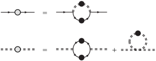
Figure 1: The diagrammatical representation of Schwinger-Dyson equations (9). The first line holds for both $\psi_{1}$ and $\psi_{2}$. The grey blobs stand for the proper self-energies, while the solid black blobs denote the full propagators. The double dashed line is for the Nambu $\Phi$ doublet.

The system of Schwinger-Dyson equations forms an infinite tower of equations for all Green’s functions of the theory. For practical calculation one usually has to truncate it at some level. We truncated it at the level of three-point Green’s functions, which we approximate by the bare ones. The resulting system of Schwinger-Dyson equations in terms of the unknown functions $\Sigma_{j}$ and $\Pi$ is

$$\begin{split}\Sigma_{1,p}&=\mathrm{i}y_{1}^{2}\int\frac{\mathrm{d}^{4}k}{(2\pi)^{4}}\frac{\Sigma_{1,k}}{k^{2}-\Sigma_{1,k}^{2}}\frac{\Pi_{k-p}}{\left[(k-p)^{2}-M^{2}\right]^{2}-|\Pi_{k-p}|^{2}}\,,\\ \Sigma_{2,p}&=\mathrm{i}y_{2}^{2}\int\frac{\mathrm{d}^{4}k}{(2\pi)^{4}}\frac{\Sigma_{2,k}}{k^{2}-\Sigma_{2,k}^{2}}\frac{\Pi^{*}_{k-p}}{\left[(k-p)^{2}-M^{2}\right]^{2}-|\Pi_{k-p}|^{2}}\,,\\ \Pi_{p}&=-\sum_{j=1,2}2\mathrm{i}y_{j}^{2}\int\frac{\mathrm{d}^{4}k}{(2\pi)^{4}}\frac{\Sigma_{j,k}}{k^{2}-\Sigma_{j,k}^{2}}\frac{\Sigma_{j,k-p}}{(k-p)^{2}-\Sigma_{j,k-p}^{2}}+\mathrm{i}\lambda\int\frac{\mathrm{d}^{4}k}{(2\pi)^{4}}\frac{\Pi_{k}}{(k^{2}-M^{2})^{2}-|\Pi_{k}|^{2}}\,.\end{split}$$ (9)

See also the diagrammatical representation of these Schwinger-Dyson equations – Fig. 1. If nonzero solutions $\Sigma_{j}$ and $\Pi$ exist, then they should necessarily be ultraviolet(UV)-finite since the corresponding counter terms are prohibited by symmetry.

Fermion masses $m_{j}$ are determined in terms of $\Sigma_{j}$ by solving

$$m_{j}^{2}=\Sigma^{2}_{j}(p^{2}=m^{2}_{j})\,.$$ (10)

By dimensional arguments the solutions must have the form

$$m_{j}=Mf_{j}(y_{1},y_{2})\,,$$ (11)

to be compared with $m_{j}=(-2M^{2}/\lambda)^{1/2}y_{j}$ in the case of a condensing $\phi$. This is the crucial point: while in the standard Higgs mechanism the functions $f_{j}$ are simple linear functions, in the present model we expect some more complicated functions, which should also be nonanalytic, because we deal with nonperturbative effects, that can not be obtained at any finite order of perturbative expansion in coupling constants $y_{j}$. Moreover there is a possibility that a small change in $y_{j}$ (say, about one order of magnitude) might produce much larger change in order of magnitude of fermion masses.

Like in the fermionic sector, the scalar spectrum can be obtained as a pole of the propagator:

$$M_{1,2}^{2}=M^{2}\pm|\Pi(p^{2}=M^{2}_{1,2})|\,.$$ (12)

This is easily interpreted: As a result of spontaneous symmetry breaking there appear two real scalar fields with different masses $M_{1,2}$, instead of one complex field with mass $M$.

Our numerical analysis confirms the existence of the nonzero solutions $\Sigma_{j}$ and $\Pi$. At present we are, however, able to say nothing about their uniqueness. Upon performing the Wick rotation we have found numerically the real solutions $\Sigma_{j}$ and $\Pi$ with the following properties: First, they vanish very fast at large $p^{2}$ (faster then any power of $p^{2}$). Second, the solutions are found so far only for large values of the Yukawa coupling constants $y_{j}$ (or, more precisely, for $y_{1}$ and $y_{2}$ not being simultaneously small). Third, fermion mass ratio $m^{2}_{1}/m^{2}_{2}$ exhibits tremendous amplification upon decent changes of $y_{1}/y_{2}$. For example, for $y_{1}/y_{2}=77.4/88$ we get $m^{2}_{1}/m^{2}_{2}=10^{-2}$. Obviously this is alluring. If justified and understood analytically, this property of the solutions of the model should not be called fine tuning. Finding the explicit form of the functions $f_{j}(y_{1},y_{2})$ in Eq. (11) is our ultimate dream.

More details on the numerics and adopted approximations can be found in the Sec. V.

III.2 Nambu-Goldstone boson

With the gauge interaction still switched off we reveal in the second step the Nambu-Goldstone (NG) excitation and compute its effective couplings with fermion and boson fields. The analysis is standard:

The conservation of the axial-vector current

$$j^{\mu}_{A}(x)=\bar{\psi}_{1}\gamma^{\mu}\gamma_{5}\psi_{1}-\bar{\psi}_{2}\gamma^{\mu}\gamma_{5}\psi_{2}+2\mathrm{i}\left[(\partial^{\mu}\phi)^{\dagger}\phi-\phi^{\dagger}\partial^{\mu}\phi\right]$$ (13)

implies the axial-vector Ward identities for the proper vertex functions:

$$\begin{split}q_{\mu}\Gamma^{\mu}_{\psi_{j}}(p+q,p)&\>=\>Q_{j}\left[S_{j}^{-1}(p+q)\gamma_{5}+\gamma_{5}S_{j}^{-1}(p)\right]\,,\\ q_{\mu}\Gamma^{\mu}_{\phi}(p+q,p)&\>=\>-2D^{-1}(p+q)\Xi+2\Xi D^{-1}(p)\,,\end{split}$$ (14)

where the proper vertex functions $\Gamma^{\mu}_{\psi_{j}}$, $\Gamma^{\mu}_{\phi}$ correspond to the Green’s functions

$$\begin{split}G_{\psi_{j}}^{\mu}(x,y,z)&\>=\>\langle 0|T\{j_{A}^{\mu}(x)\psi_{j}(y)\bar{\psi}_{j}(z)\}|0\rangle\,,\\ G_{\phi}^{\mu}(x,y,z)&\>=\>\langle 0|T\{j_{A}^{\mu}(x)\Phi(y)\Phi^{\dagger}(z)\}|0\rangle\end{split}$$ (15)

with the full propagators of the external legs cut off. The matrix $\Xi$,

$$\Xi=\left(\begin{array}[]{cr}1&0\\ 0&-1\end{array}\right),$$ (16)

operates in the $\phi-\phi^{\dagger}$ space and is quite analogous to $\gamma_{5}$ in the fermion sector.

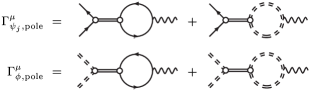
Figure 2: The diagrammatical representation of pole parts of proper vertices $\Gamma^{\mu}_{\psi_{j}}$ and $\Gamma^{\mu}_{\phi}$ (17). The pole itself is interpreted as a propagator of intermediate massless scalar particle – the Nambu-Goldstone boson, depicted by solid double line. The small empty circles are vertices $P_{\psi_{j}}$, $P_{\phi}$ (III.2). The external vector boson lines are indicated for the case the $U(1)_{A}$ symmetry was gauged.

For $\Sigma_{j}$ and $\Pi$ different from zero these identities imply that the proper vertices themselves develop poles for $q^{2}\rightarrow 0$:

$$\begin{split}\Gamma^{\mu}_{\psi_{j},\mathrm{pole}}(p+q,p)&\>=\>\frac{q^{\mu}}{q^{2}}Q_{j}\left[S_{j}^{-1}(p+q)\gamma_{5}+\gamma_{5}S_{j}^{-1}(p)\right]\,,\\ \Gamma^{\mu}_{\phi,\mathrm{pole}}(p+q,p)&\>=\>\frac{q^{\mu}}{q^{2}}\left[-2D^{-1}(p+q)\Xi+2\Xi D^{-1}(p)\right]\,.\end{split}$$ (17)

In fact the poles are nothing but the manifestation of the presence of the NG boson, see Fig. 2. These identities also allow to explicitly compute the interaction vertices of the NG boson with the fermions and scalars; for the details see Ref. Brauner and Hošek (2005), the result is [within the Ansatz (8)]

$$\!\!\!\!\!\!\!\!\hphantom{{}_{\phi}}P_{\psi_{j}}(p+q,p)=-\frac{Q_{j}}{N}\left[\Sigma_{j}(p+q)+\Sigma_{j}(p)\right]\gamma_{5}\,,$$

$$\!\!\!\!\!\!\!\!\hphantom{{}_{\psi_{j}}}P_{\phi}(p+q,p)=$$ (21)

$$-\frac{2}{N}\left(\begin{array}[]{cc}0&\Pi(p+q)+\Pi(p)\\ -\Pi^{*}(p+q)-\Pi^{*}(p)&0\end{array}\right)\,.$$

The normalization factor $N$ can be expressed as

$$N=\sqrt{J_{\psi_{1}}(0)+J_{\psi_{2}}(0)+J_{\phi}(0)}\,,$$ (22)

where the functions $J_{\psi_{j}}$ and $J_{\phi}$ are defined by

$$\begin{split}-\mathrm{i}q^{\mu}J_{\psi_{j}}(q^{2})&=8\int\frac{\mathrm{d}^{4}k}{(2\pi)^{4}}\frac{(k-q)^{\mu}\Sigma_{j,k}}{k^{2}-\Sigma^{2}_{j,k}}\frac{\Sigma_{j,k}+\Sigma_{j,k-q}}{(k-q)^{2}-\Sigma^{2}_{j,k-q}}\,,\\ -\mathrm{i}q^{\mu}J_{\phi}(q^{2})&=8\int\frac{\mathrm{d}^{4}k}{(2\pi)^{4}}\frac{(2k-q)^{\mu}(k^{2}-M^{2})}{(k^{2}-M^{2})^{2}-|\Pi_{k}|^{2}}\frac{\mathop{\rm Re}\nolimits\left[\Pi^{*}_{k-q}\bigl{(}\Pi_{k}+\Pi_{k-q}\bigr{)}\right]}{\bigl{[}(k-q)^{2}-M^{2}\bigr{]}^{2}-|\Pi_{k-q}|^{2}}\,.\end{split}$$ (23)

IV Local Symmetry

IV.1 Gauge boson mass

In this step we switch on the gauge interaction perturbatively and compute the axial-vector gauge boson mass squared as a residue at the massless pole of the gauge field polarization tensor $\Pi^{\mu\nu}(q)$. As in other strongly coupled models in which the NG boson is a composite Eidelman et al. (2004); Freundlich and Lurie (1970); Jackiw and Johnson (1973); Cornwall and Norton (1973); Gribov (1994); Tanabashi et al. (1989) we are only able to compute the longitudinal part of $\Pi^{\mu\nu}$ due to the bilinear coupling of NG boson with gauge boson – see Fig. 3.

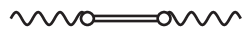
Figure 3: The effective bilinear coupling of NG boson with gauge boson, giving rise to the longitudinal polarisation of the latter and hence generating its mass. The bilinear coupling is induced by the couplings of NG boson with fermionic and scalar fields $P_{\psi_{j}}$ and $P_{\phi}$, compare with Fig. 2.

Insisting on transversality of $\Pi^{\mu\nu}$ due to the axial-vector current conservation, we conclude that the gauge boson mass squared is softly generated in terms of $\Sigma_{j}$ and $\Pi$ as

$$M_{A}^{2}=g^{2}[I_{\psi_{1}}(0)+I_{\psi_{2}}(0)+I_{\phi}(0)]\,,$$ (24)

where

$$\begin{split}\mathrm{i}q^{\nu}I_{\psi_{j}}(q^{2})&=4\int\frac{\mathrm{d}^{4}k}{(2\pi)^{4}}\frac{\left[(k+q)^{\nu}\Sigma_{j,k}-k^{\nu}\Sigma_{j,k+q}\right]\left[\Sigma_{j,k+q}+\Sigma_{ji,k}\right]}{\Big{[}(k+q)^{2}-\Sigma_{j,k+q}^{2}\Big{]}\Big{[}k^{2}-\Sigma_{j,k}^{2}\Big{]}}\,,\\ \mathrm{i}q^{\nu}I_{\phi}(q^{2})&=-2\int\frac{\mathrm{d}^{4}k}{(2\pi)^{4}}\frac{(2k+q)^{\nu}\Big{\{}[\Pi_{k+q}+\Pi_{k}]\left[[(k+q)^{2}-M^{2}]\Pi^{*}_{k}-(k^{2}-M^{2})\Pi^{*}_{k+q}\right]+\mathrm{c.c.}\Big{\}}}{\Big{[}[(k+q)^{2}-M^{2}]^{2}-|\Pi_{k+q}|^{2}\Big{]}\Big{[}(k^{2}-M^{2})^{2}-|\Pi_{k}|^{2}\Big{]}}\,.\end{split}$$ (25)

For $q^{2}=0$ we have explicitly

$$\begin{split}I_{\psi_{j}}(0)&=-8\mathrm{i}\int\frac{\mathrm{d}^{4}k}{(2\pi)^{4}}\frac{\Sigma_{j,k}\left[\Sigma_{j,k}-2k^{2}\frac{\mathrm{d}}{\mathrm{d}k^{2}}\Sigma_{j,k}\right]}{\Big{[}k^{2}-\Sigma_{j,k}^{2}\Big{]}^{2}}\,,\\ I_{\phi}(0)&=16\mathrm{i}\int\frac{\mathrm{d}^{4}k}{(2\pi)^{4}}\frac{k^{2}|\Pi_{k}|\left[|\Pi_{k}|-(k^{2}-M^{2})\frac{\mathrm{d}}{\mathrm{d}k^{2}}|\Pi_{k}|\right]}{\Big{[}(k^{2}-M^{2})^{2}-|\Pi_{k}|^{2}\Big{]}^{2}}\,.\end{split}$$ (26)

In the weakly coupled Higgs model with the elementary ‘would-be’ NG boson the spontaneous gauge boson mass generation is more transparent: The polarization tensor $\Pi^{\mu\nu}(q)$ can easily be computed completely Englert and Brout (1964) and decent behavior of scattering amplitudes with longitudinally polarized massive gauge bosons can be illustrated explicitly.

On the other hand, in strongly coupled models the lack of the bound-state spectrum apart from the NG sector guaranteed by the existence theorem of Goldstone implies: First, the $g^{\mu\nu}$ part of the polarization tensor can hardly be computed. Second, decent behavior of scattering amplitudes with longitudinally polarized massive gauge bosons cannot be determined from first principles.

IV.2 $A^{3}$ vertex

The spontaneous breakdown of the Abelian gauge chiral symmetry found in the low-momentum behavior of propagators should by construction manifest in noninvariant loop-generated vertices. Being ultraviolet-finite they represent the genuine quantum-field theory predictions of the suggested nonperturbative approach. In the Abelian prototype presented here it suffices to provide one illustrative (still gedanken) example:

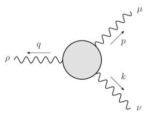
Figure 4: The full $A^{3}$ vertex, denoted in the main text as $\mathrm{i}T^{\mu\nu\rho}(p,k)$. Energy-momentum conservation is assumed: $p+k+q=0$.

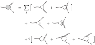
Figure 5: Diagrammatical representation of the expression (IV.2). Each diagram has the same assignment of momenta $p$, $k$, $q$ and Lorentz indices $\mu$, $\nu$, $\rho$ as the full vertex in Fig. 4. The symmetry factors are indicated explicitly.

The gauge interaction of $A^{\mu}$ with the massive fermions gives rise to the effective $A^{3}$ vertex depicted in Fig. 4. Up to $g^{3}$ the result (calculated as a proper vertex) can be written as the following sum (compare with Fig. 5)

$$\mathrm{i}T^{\mu\nu\rho}(p,k)=$$

$$\sum_{j}\Big{[}\mathrm{i}T^{\mu\nu\rho}_{\psi_{j}}(p,k)+\mathrm{i}T^{\nu\mu\rho}_{\psi_{j}}(k,p)\Big{]}$$

$${}+\mathrm{i}T^{\mu\nu\rho}_{\Phi}(p,k)+\mathrm{i}T^{\nu\mu\rho}_{\Phi}(k,p)$$

$${}+2\Big{[}\mathrm{i}T^{\mu\nu\rho}_{4}(p,k)+\mathrm{i}T^{\mu\rho\nu}_{4}(p,-p-k)+\mathrm{i}T^{\nu\rho\mu}_{4}(k,-p-k)\Big{]}\,,$$

where (with the $\mathrm{i}0^{+}$’s suppressed)

$$\begin{split}\mathrm{i}T^{\mu\nu\rho}_{\psi_{j}}(p,k)&\>=\>g^{3}Q_{j}^{3}\int\frac{\mathrm{d}^{4}\ell}{(2\pi)^{4}}\frac{1}{\left[\ell^{2}-\Sigma_{j,\ell}^{2}\right]\left[(\ell+p)^{2}-\Sigma_{j,\ell+p}^{2}\right]\left[(\ell-k)^{2}-\Sigma_{j,\ell-k}^{2}\right]}\times\\ &\hphantom{\>=\>}\Big{\{}\mathop{\rm Tr}\nolimits[\gamma^{\mu}\not{\ell}\gamma^{\nu}(\not{\ell}-\not{k})\gamma^{\rho}(\not{\ell}+\not{p})\gamma_{5}]+\\ &\hphantom{\>=\>\{}-\,4\mathrm{i}\epsilon^{\mu\nu\rho}_{\hphantom{\mu\nu\rho}\sigma}\left[\ell^{\sigma}\Sigma_{j,\ell+p}\Sigma_{j,\ell-k}+(\ell+p)^{\sigma}\Sigma_{j,\ell}\Sigma_{j,\ell-k}+(\ell-k)^{\sigma}\Sigma_{j,\ell}\Sigma_{j,\ell+p}\right]\Big{\}}\,,\\ \mathrm{i}T^{\mu\nu\rho}_{\Phi}(p,k)&\>=\>g^{3}\!\!\int\!\frac{\mathrm{d}^{4}\ell}{(2\pi)^{4}}\frac{(2\ell+p)^{\mu}(2\ell-k)^{\nu}(2\ell+p-k)^{\rho}}{[(\ell^{2}-M^{2})^{2}-|\Pi_{\ell}|^{2}]\big{[}\left((\ell+p)^{2}-M^{2}\right)^{2}-|\Pi_{\ell+p}|^{2}\big{]}\big{[}\left((\ell-k)^{2}-M^{2}\right)^{2}-|\Pi_{\ell-k}|^{2}\big{]}}\times\\ &\hphantom{\>=\>}\Big{\{}(\ell^{2}-M^{2})^{2}\left[\Pi_{\ell+p}^{*}\Pi_{\ell-k}-\mathrm{c.c.}\right]+\\ &\hphantom{\>=\>\{}+\!\left[(\ell+p)^{2}-M^{2}\right]^{2}\left[\Pi_{\ell-k}^{*}\Pi_{\ell}-\mathrm{c.c.}\right]+\left[(\ell-k)^{2}-M^{2}\right]^{2}\left[\Pi_{\ell}^{*}\Pi_{\ell+p}-\mathrm{c.c.}\right]\Big{\}}\,,\\ \mathrm{i}T^{\mu\nu\rho}_{4}(p,k)&\>=\>4g^{3}\int\frac{\mathrm{d}^{4}\ell}{(2\pi)^{4}}\frac{g^{\mu\nu}(2\ell+p-k)^{\rho}\left[\Pi_{\ell+p}^{*}\Pi_{\ell-k}-\mathrm{c.c.}\right]}{\big{[}\left((\ell+p)^{2}-M^{2}\right)^{2}-|\Pi_{\ell+p}|^{2}\big{]}\big{[}\left((\ell-k)^{2}-M^{2}\right)^{2}-|\Pi_{\ell-k}|^{2}\big{]}}\,.\end{split}$$ (28)

Being a combination of three axial vectors, the amplitude should change its sign under the operation of parity. Indeed it does: in the fermionic contributions it is due to the presence of the Levi-Civita tensor, while in the scalar contributions it is due to the following behavior of the scalar self-energy under parity:

$$\Pi\stackrel{{\scriptstyle\mathcal{P}}}{{\rightarrow}}\Pi^{*}\,.$$ (29)

For illustration, let us now evaluate the amplitude $\mathrm{i}T^{\mu\nu\rho}(p,k)$ under certain approximations. First, we set the self-energies to be some constants. Note that the integrals remain perfectly UV finite. In fact, the scalar integrals vanish, while the quadratic divergences in the fermion integrals cancel each other since

$$\sum_{j}Q_{j}^{3}=0$$ (30)

(this, together with the requirement $\sum_{j}Q_{j}=0$, is precisely the condition for the axial anomaly to vanish). The linear divergences cancel because of the symmetric integration. Note that within this approximation the result is exactly the same as in the Higgs mechanism since we totally omit the nontrivial structure of the propagators, represented by nonconstant self-energies, and approximate them by the pole contribution. Second, for the sake of simplicity, we put all external momenta on their mass-shell:

$$p^{2}=k^{2}=q^{2}=M_{A}^{2}\,.$$ (31)

The energy-momentum conservation enables us to easily compute the dot products of external momenta:

$$p\cdot k=p\cdot q=k\cdot q=-\frac{1}{2}M_{A}^{2}\,.$$ (32)

Constant fermion self-energies turn out to be the masses: $\Sigma_{j}(p^{2})=\mathrm{const.}=m_{j}$. The resulting amplitude reads

$$\mathrm{i}T^{\mu\nu\rho}(p,k)=G\left[p^{\mu}\epsilon^{\nu\rho}_{\hphantom{\nu\rho}\alpha\beta}-k^{\nu}\epsilon^{\mu\rho}_{\hphantom{\mu\rho}\alpha\beta}-(p+k)^{\rho}\epsilon^{\mu\nu}_{\hphantom{\mu\nu}\alpha\beta}\right]p^{\alpha}k^{\beta}\,,$$ (33)

or equivalently

$$\mathrm{i}T^{\mu\nu\rho}(p,k)=G\left[(q^{\mu}k^{\alpha}-k^{\mu}q^{\alpha})p^{\beta}\epsilon^{\nu\rho}_{\hphantom{\nu\rho}\alpha\beta}+(p^{\nu}q^{\alpha}-q^{\nu}p^{\alpha})k^{\beta}\epsilon^{\rho\mu}_{\hphantom{\rho\mu}\alpha\beta}+(k^{\rho}p^{\alpha}-p^{\rho}k^{\alpha})q^{\beta}\epsilon^{\mu\nu}_{\hphantom{\mu\nu}\alpha\beta}\right]\,.$$ (34)

The latter form is perhaps more convenient because the invariance under exchange

$$(p,\mu)\leftrightarrow(k,\nu)\leftrightarrow(q,\rho)$$ (35)

is more apparent. The amplitude (34) can be generated via the following effective Lagrangian:

$$\mathcal{L}_{\rm{eff}}=G\,\epsilon_{\alpha\beta\gamma\delta}(\partial_{\sigma}A^{\alpha})(\partial^{\beta}A^{\sigma})(\partial^{\gamma}A^{\delta})\,.$$ (36)

Note that in the result (34) there are no terms proportional to $\epsilon^{\mu\nu\rho}_{\hphantom{\mu\nu\rho}\sigma}$, although they are present in the original $\mathrm{i}T^{\mu\nu\rho}_{\psi_{j}}$ [see (28)]. This is a simple consequence of the restriction $p^{2}=k^{2}=q^{2}$, for in this case there is no way how to write down any nontrivial linear combination of terms $\epsilon^{\mu\nu\rho}_{\hphantom{\mu\nu\rho}\sigma}p^{\sigma}$, $\epsilon^{\mu\nu\rho}_{\hphantom{\mu\nu\rho}\sigma}k^{\sigma}$ and $\epsilon^{\mu\nu\rho}_{\hphantom{\mu\nu\rho}\sigma}q^{\sigma}$ which would be invariant under the exchange (35). For general momenta $p^{2}\neq k^{2}\neq q^{2}$ these terms would be present.

The effective coupling constant $G$ can be expressed as

$$G=g^{3}\sum_{j}Q_{j}^{3}f(m_{j}^{2},M_{A}^{2})\,.$$ (37)

The function $f$ is defined by the integral

$$f(m^{2},M^{2})=\frac{2}{\pi^{2}M^{2}}\int_{0}^{1}\mathrm{d}z\frac{z(1-z)}{\sqrt{z(3z-4)+\frac{4m^{2}}{M^{2}}}}\arctan\frac{z}{\sqrt{z(3z-4)+\frac{4m^{2}}{M^{2}}}}$$ (38)

(here $m^{2}$ should be replaced by $m^{2}-\mathrm{i}0^{+}$ whenever the correct branch choice of a multivalued analytic function is in question), which can be calculated analytically in some special cases:

$$\begin{split}f(m^{2},0)&\>=\>\frac{1}{24\pi^{2}m^{2}}\,,\\ f(0,M^{2})&\>=\>\frac{-1}{6\pi^{2}M^{2}}\,.\end{split}$$ (39)

More information about the shape of $f$ can be extracted numerically – see Fig. 6.

Figure 6: The $M^{2}$-dependence of the function $f(m^{2},M^{2})$. Both quantities are normalized by $m^{2}$ to be dimensionless; note that $m^{2}f(m^{2},M^{2})$ is only function of $M^{2}/m^{2}$. The cusps appear at $M^{2}=3m^{2}$ and $M^{2}=4m^{2}$. The former one also indicates the beginning of the imaginary part.

V Numerics

In this section the results of the numerical solution of Schwinger-Dyson equations (9) are presented. Moreover, as we consider the results quite interesting and important, the description of the numerical procedure together with discussion of its stability is presented.

V.1 Numerical results

The system of equations (9) is quite difficult to be solved even numerically, so certain approximations have to be done. First, we switch to the Euclidean metric via the Wick rotation. By this we get rid of some poles in the fermionic and scalar propagators. The absence of poles makes numerical integration much easier. Moreover, one can consider the self-energies to be real, without loss of generality. Note, however, that not all poles are removed, namely the pole in the scalar propagator remains: It takes place if $\Pi(p^{2})=p^{2}+M^{2}$ for some $p^{2}$.

Second, we set $\lambda=0$. In fact, in the present model the $\lambda$-term is not of high importance for the mass generation. In the Higgs case the scalar self-interaction is of utmost importance: It fixes the numerical value of the condensate and stabilizes the scalar field energy. In our case both reasons for considering $\lambda\neq 0$ are clearly absent. However, in full treatment including the perturbative effects of renormalization yet to be done the term $\frac{1}{2}\lambda(\phi^{\dagger}\phi)^{2}$ will become indispensable as a counter term.

As a net result, we solve the following set of equations for the unknown functions $\Sigma_{1}(p^{2})$, $\Sigma_{2}(p^{2})$ and $\Pi(p^{2})$:

$$\begin{split}\Sigma_{1,p}&\>=\>y_{1}^{2}\int\frac{\mathrm{d}^{4}k}{(2\pi)^{4}}\frac{\Sigma_{1,k}}{k^{2}+\Sigma_{1,k}^{2}}\frac{\Pi_{k-p}}{\left[(k-p)^{2}+M^{2}\right]^{2}-\Pi_{k-p}^{2}}\,,\\ \Sigma_{2,p}&\>=\>y_{2}^{2}\int\frac{\mathrm{d}^{4}k}{(2\pi)^{4}}\frac{\Sigma_{2,k}}{k^{2}+\Sigma_{2,k}^{2}}\frac{\Pi_{k-p}}{\left[(k-p)^{2}+M^{2}\right]^{2}-\Pi_{k-p}^{2}}\,,\\ \Pi_{p}&\>=\>\sum_{j=1,2}2y_{j}^{2}\int\frac{\mathrm{d}^{4}k}{(2\pi)^{4}}\frac{\Sigma_{j,k}}{k^{2}+\Sigma_{j,k}^{2}}\frac{\Sigma_{j,k-p}}{(k-p)^{2}+\Sigma_{j,k-p}^{2}}\,,\end{split}$$ (40)

where $p^{2}=p_{0}^{2}+p_{1}^{2}+p_{2}^{2}+p_{3}^{2}\geq 0$.

The solutions can be classified with respect to the pairs of coupling constants $(y_{1},y_{2})$. The mass parameter $M$ is not relevant, since as the only parameter with dimension of mass in the theory it serves just as a scale parameter for the self-energies and momenta. The typical shape of the resulting self-energies is depicted in Fig. 7. They are saturated at low momenta and fall down rapidly at high momenta. Using logarithmic scale on $y$-axis in Fig. 7 it would be apparent that the self-energies fall down actually faster then any power of $p^{2}$.

Figure 7: Typical shape of the solutions $\Sigma_{1}(p^{2})$, $\Sigma_{2}(p^{2})$ and $\Pi(p^{2})$ to the system of equations (40), computed here for Yukawa coupling constants $y_{1}=83$ and $y_{2}=88$. Note the saturation of the self-energies at low momenta and fast decrease at high momenta.

We have found interesting qualitative differences between the solutions of Eq. (40) for different values $(y_{1},y_{2})$. The main results are summarised in Fig. 8. There is an area in the $(y_{1},y_{2})$ plane, located around the axis $y_{1}=y_{2}$ and denoted as $(\mathbb{II})$, where both $\Sigma_{1}$ and $\Sigma_{2}$ are nonzero, and areas where only one of them, $\Sigma_{1}$ or $\Sigma_{2}$, is nonzero [areas $(\mathbb{I})$ and $(\mathbb{III})$]. There is also an area $(\mathbb{IV})$ where the pole in the scalar propagator, mentioned earlier, matters. The self-energies (which are expected to be imaginary here) were not computed in this area, we do not know anything about their behavior here.

Figure 8: The $(y_{1},y_{2})$ plane with indicated areas of different behavior of the system of equations (40). According to the resulting fermion self-energies there are three main areas: first where $\Sigma_{1}=0$ and $\Sigma_{2}\neq 0$, second where $\Sigma_{1}\neq 0$ and $\Sigma_{2}\neq 0$ and third where $\Sigma_{1}\neq 0$ and $\Sigma_{2}=0$, denoted as $(\mathbb{I})$, $(\mathbb{II})$ and $(\mathbb{III})$, respectively. There is also another important area, denoted as $(\mathbb{IV})$, where the pole in the scalar propagator takes place (and hence the imaginary parts of the self-energies are expected to appear). However we do not know anything about behavior of the self-energies in this area because of difficulties when numerically integrating the pole. The dashed line, going from $y_{1}=72$ and $y_{2}=88$ to $y_{1}=104$ and $y_{2}=88$, shows where the dependence of the spectrum on the Yukawa coupling constants was probed – see Fig. 9 and Fig. 10.

Our aim was to find the dependence of the spectrum – the masses of the fermions, scalar bosons and the vector boson – on the Yukawa coupling constants $y_{1}$ and $y_{2}$ [or, more precisely, on absolute values $|y_{1}|$ and $|y_{2}|$, due to the shape of the Schwinger-Dyson equations (40)]. For the calculation of masses we have used Eqs. (10), (12), (24), in the case of vector boson Wick rotated to the Euclidean metric. We have probed the $y_{1,2}$-dependence along the cut depicted in Fig. 8, since it connects all the three main areas $(\mathbb{I})$, $(\mathbb{II})$ and $(\mathbb{III})$ and therefore the resulting $y_{1,2}$-dependence of the spectrum can be regarded as quite typical. The results are depicted in Fig. 9 and Fig. 10. Note how the critical lines between the areas are evident in the $y_{1,2}$-dependence of the spectrum. The most significant result – the behavior of the fermionic spectrum – can be seen in Fig. 10. As $y_{1}$ approaches the critical line between $(\mathbb{II})$ and $(\mathbb{I})$ [or $(\mathbb{III})$, respectively] in the direction from $(\mathbb{II})$ to $(\mathbb{I})$ [$(\mathbb{III})$], the ratio $m^{2}_{2}/m^{2}_{1}$ becomes arbitrarily high (low)!

Figure 9: The $y_{1}$-dependence of the scalar masses $M^{2}_{1,2}$ with fixed $y_{2}=88$.

Figure 10: The $y_{1}$-dependence of the fermion and vector boson masses $m^{2}_{1,2}$ and $M^{2}_{A}$ with fixed $y_{2}=88$.

V.2 Numerical procedure

Let us now say more about the numerical procedure itself. More formally, we have to solve the following set of equations:

$$\begin{split}\Sigma_{1}&\>=\>F_{1}[\Sigma_{1},\Pi]\,,\\ \Sigma_{2}&\>=\>F_{2}[\Sigma_{2},\Pi]\,,\\ \Pi&\>=\>G[\Sigma_{1},\Sigma_{2}]\,,\end{split}$$ (41)

where $F_{j}$, $G$ are some functionals. To solve this system, we have adopted the method of iterations. After choosing some initial Ansatz for $\Sigma$’s:

$$\Sigma_{1}^{(0)},\Sigma_{2}^{(0)}$$ (42)

and calculating also the ‘zeroth’ iteration of the $\Pi$:

$$\Pi^{(0)}=G[\Sigma_{1}^{(0)},\Sigma_{2}^{(0)}]\,,$$ (43)

the iterating process is established: ($n\geq 1$)

$$\begin{split}\Sigma_{1}^{(n)}&\>=\>F_{1}[\Sigma_{1}^{(n-1)},\Pi^{(n-1)}]\,,\\ \Sigma_{2}^{(n)}&\>=\>F_{2}[\Sigma_{2}^{(n-1)},\Pi^{(n-1)}]\,,\\ \Pi^{(n)}&\>=\>G[\Sigma_{1}^{(n-1)},\Sigma_{2}^{(n-1)}]\,.\end{split}$$ (44)

If this procedure converges, we have the solution. In order to control the convergence we used the quantity

$$I^{(n)}=\frac{\int X^{(n)}}{\int X^{(n-1)}}\,,$$ (45)

where $X$ stands for any of $\Sigma_{j}$, $\Pi$. If $I^{(n)}\to 1$, we considered $X^{(n)}$ to be the solution. This simple criterion is sufficient in our case because the functions $X^{(n)}$ turn out to be well behaved: there are no intersections between distinct iterations, or, loosely speaking, their shapes are similar, the only changes are in their ‘size’ (at least in the nonasymptotic region).

Usual behavior of such a nonlinear system in the case of only one equation for one unknown function (for instance an equation for $\Sigma$ with $\Pi$ set to be a constant) is such that for any initial Ansatz the iteration procedure converges to some solution. The solution may be trivial (i.e. $I^{(n)}<1$, $I^{(n)}\nrightarrow 1$) or nontrivial (i.e. $I^{(n)}\to 1$), depending whether $y<y_{\mathrm{crit}}$ or $y>y_{\mathrm{crit}}$, respectively, for some critical value $y_{\mathrm{crit}}$.

In our case of more coupled equations the situation is, however, different. Having some fixed Ansatz, there are three possibilities: (1) The iteration procedure converges to the trivial solution [which exists always for all $(y_{1},y_{2})$]. (2) It blows up (i.e. $I^{(n)}>1$, $I^{(n)}\nrightarrow 1$). (3) It converges to a nontrivial solution (if it exists), depending on the $(y_{1},y_{2})$ (see Fig. 8).

This behavior clearly depends on the Ansatz. To be specific, our class of Ansätze consisted of functions

$$\Sigma_{1}^{(0)}(p^{2})=\Sigma_{2}^{(0)}(p^{2})=x\frac{M^{5}}{(p^{2}+M^{2})^{2}}$$ (46)

with $x$ being a free parameter. For $x$ too small or too large the iteration procedure goes to the trivial solution or blows up, respectively. Properly adjusting the value of $x$ between these two extremes one can manage that the iteration procedure converges to the nontrivial solution.

V.3 Numerical stability

A special care was taken to check whether the numerical procedure is stable in the sense that its results (especially the strong $y_{1,2}$-dependence of the fermion masses) remain unchanged upon the changes of the numerical algorithm. We tested four main variations of the algorithm:

Class of Ansätze

Besides (46) we considered also other Ansatz classes, all functions decreasing as some power of $p^{2}$ or exponentially, respectively. For some of them (some very rapidly decreasing exponentials) it was not possible to adjust the variable $x$ [see (46)] to converge to any but the trivial solution. For the other Ansatz classes, however, the results were nontrivial and they all coincided.

Step size

There is, of course, a step size dependence of the numerical integration results, the important question is, however, how this dependence behaves for arbitrarily small step sizes. If there is no sensible (i.e. finite) limit of the integral as the step sizes are going to zero (the continuum limit), the results of the numerical integration have no meaning. We checked that this limit does exist and that all described phenomena, especially the strong $y_{1,2}$-dependence of the fermion masses, are present in it.

Integration method

Having expressed the integral equations (40) in the hyperspherical coordinates, we can do two angular integrations analytically. The two remaining integrations (one over momentum and one angular) must be performed numerically. For this purpose we employed consecutively the trapezoidal rule and the Simpson’s rule, for the angular integration also the Gauss-Chebyshev quadrature formula (using Chebyshev polynomials of the second kind). The final results for all integration methods agreed, the differences were only in the step size dependence, i.e. in the speed of convergence to the continuum limit.

Momentum cut-off

Since the momentum integral is over the infinite interval, for the purposes of the numerical integration a momentum cut-off must be introduced. However it turns out that one does not need to check the cut-off dependence of the results. That is because the resulting self-energies are so rapidly decreasing that the contribution from the high momenta is negligible.

Moreover, in order to check the consistency of our numerical method by a comparison with an independent result, we calculated the equation for $\Sigma_{j}$ [see (40)] with $\Pi$ set to be a constant [up to our knowledge, there are no independent calculations of the full set of the coupled equations (40) we could compare with] and compared our result with the results of Sauli et al. (2006) [Eq. (2.11) and Fig. 3 therein]. They coincided.

VI Concluding remarks and outlook

Within the effective quantum field theory for electroweak interactions at forthcoming energy scale we find the use of scalar fields still welcome: Their Yukawa couplings with massless elementary fermion fields break explicitly the huge chiral symmetries of three electroweakly identical fermion families exactly to the sanctified $SU(2)_{L}\times U(1)_{Y}$. Alternatives without scalars struggle with guaranteeing unobservability of physical consequences of these unwanted symmetries.

Linear dependences of the wildly wide, sparse and irregular fermion mass spectrum upon the Yukawa coupling constants of the Standard model are, however, a drawback. It is feasible that the fermion masses can be generated by the Yukawa interactions dynamically without ever referring to the scalar field condensation Imry (1970); Tanabashi et al. (1989). In such a case the dependences of the fermion masses upon the Yukawa coupling constants would be nonanalytic. In an Abelian prototype we have provided a bona fide indication that this is possible. Most importantly, we have convincingly demonstrated that a small change in the ratio of the Yukawa couplings may lead to an orders-of-magnitude change in the ratio of the generated fermion masses. We hope that this mechanism could provide a natural explanation of the hierarchy of fermion masses in the Standard model.

The price we pay is that the Yukawa interactions having the expected properties must be strong. But we are accustomed to live with QCD strongly interacting at large distances even though we still don’t know how to solve it (incidentally, apart from the NG sector). We are tempted to interpret our findings as manifestations of nontrivial fixed points Wilson (1971) in our model.

The bonus we get is an interesting relation of fermion and gauge boson mass generation mechanisms. Indeed, in contrast with the Higgs mechanism in our case for the Yukawa couplings set to zero both fermion and gauge boson masses vanish.

We are confident that with some technical modifications the generalization of the Abelian mechanism presented above to $SU(2)_{L}\times U(1)_{Y}$ can be done Brauner and Hošek (2004). Whether it can be converted into a phenomenologically viable alternative of the Standard model remains, however, to be seen.