S. Abdullina, D. Acostab, P. Bartalinib, R. Cavanaughb, A. Drozdetskiyeb, G. Karapostolic, G. Mitselmakherb, Yu. Pakhotinb, B. Scurlockb, M. Spiropulud eCorresponding author, e-mail: Alexey.Drozdetskiy@cern.ch aFermi National Laboratory, Chicago, IL, USA bUniversity of Florida, Gainesville, FL, USA cCERN and University of Athens, Greece dCERN

This paper presents GARCON program, illustrating its functionality on a simple HEP analysis example. The program automatically performs rectangular cuts optimization and verification for stability in a multi-dimensional phase space. The program has been successfully used by a number of very different analyses presented in the CMS Physics Technical Design Report. The current version GARCON 2.0 incorporates the feedback the authors have received. User’s Manual is included as a part of the note.

1 Introduction

Genetic algorithm (GA) definitions along with some review information are given in Ref. [1]. In short, GA is a set of algorithms inspired by concepts of natural selection with evolving individuals, which allowed to be created randomly, to mutate, inherit their qualities, etc. useful in optimization problems with a large number of discrete solutions.

Typically, a High Energy Physics (HEP) analysis has quite a few selection criteria (cuts) to optimize for example a significance of the “signal” excess over “background” events: transverse energy/momenta cuts, missing transverse energy, angular correlations, isolation and impact parameters, etc. In such cases simple scan over multi-dimensional cuts space (especially when done on top of a scan over theoretical predictions parameters space, e.g. for SUSY) leads to CPU time demand varying from days to many years… One of the alternative methods, which solves the issue is to employ a Genetic Algorithm, see e.g. [2, 3, 4].

We wrote a code, GARCON [5], which automatically performs cut optimization and verification for stability effectively trying $\sim 10^{50}$ cut set parameters/values permutations for millions of input events in hours time scale. Examples of analyses with GARCON can be found presented in the CMS Physics TDR, v.2 [6] and in recent papers [7, 8, 9].

In comparison with other automated optimization methods GARCON output is transparent to user: it just says what rectangular cut values are optimal and recommended in an analysis. An interpretation of these cut values is absolutely the same as when one selects a set of rectangular cut values for each variable in a “classical” way “by eye”, except in the case of GARCON those cut values would be optimal to deliver the best value of the function used for optimization.

In this paper we describe the basics of the GA, illustrating GARCON functionality on a simple example of a “toy” MC generator-level analysis. A significant part of the paper consists of User’s Manual describing how to use the program (Sec. 5).

GARCON version 2.0 [5] among many other features allows user:

• to select an optimization function among known significance estimators, as well as to define user’s own criteria, which may be as simple as signal to background ratio, or more complicated, including different systematic uncertainties separately on signal and background processes, different weights per event, etc.;

• to define a precision of the optimization;

• to restrict the optimization using different kind of requirements, such us minimum number of signal/background events to survive after final cuts, variables/processes to be used for a particular optimization run, number of optimizations inside one run to ensure that optimization converges/finds not just a local maximum(s), but a global one as well (in case of a complicated phase space);

• to automatically verify stability of results.

This paper has the following structure:

• Section 2 describes details of a “toy”-study example,

• Section 3 shows a simple example of a “classical”, eye-balling approach analysis for cuts optimization,

• Section 4 gives details on a GARCON, GA approach to cuts optimization and contains a comparison of these two approaches,

• the following section is a detailed how-to user’s manual.

The chosen “toy-study” is on purpose a simple Monte Carlo (MC) analysis to illustrate GARCON functionality in a clear and transparent way. Much more sophisticated use-cases of the program can be found elsewhere [7, 8, 9].

2 LM6 with PYTHIA: a Toy Study

We are working in the framework of mSUGRA model [10] which is derived from more general MSSM  [11] model using constrains inspired by the super-gravity unification. In case of mSUGRA, the number of independent MSSM parameters is reduced to just five. For our illustration we selected a point in mSUGRA parameter space with the following values of mSUGRA parameters:

• the universal gaugino mass $m_{1/2}=400$ GeV,

• the scalar mass $m_{0}=85$ GeV,

• the trilinear soft supersymmetry-breaking parameter $A_{0}=0$,

• the ratio of Higgs vacuum expectation values, $\tan\beta=10$,

• sign of Higgsino mixing parameter, $sign(\mu)>0$.

Characteristic qualities of SUSY events, following from a consideration of signal Feynman diagrams are: large MET (mainly due to massive stable SUSY particles, LSP) and large jet E_Ts (due to heavy SUSY particles cascade decays).

Background processes considered in this study are QCD, W/Z+jets, double weak-boson production and $t\bar{t}$.

The main generation tool is PYTHIA 6.227 [12]. In addition, ISASUGRA, part of ISAJET 7.69 [13] is linked to PYTHIA to provide mSUGRA masses, couplings and branchings for the signal simulation.

All simulations and analysis is done for an integrated luminosity of $10fb^{-1}$.

2.1 Parameters of generation

PYTHIA parameters for all generated processes are those for underlying events. These parameters are specially tuned for LHC and used by both ATLAS and CMS collaborations, defining underlying event physics can be found elsewhere [14]. The simulation of the processes with large cross-sections is performed in certain intervals of $\hat{\rm p}_{\rm T}$. The list of simulated processes and their main characteristics are listed in Table 1.

Table 1: Data samples and their parameters

	PYTHIA Process id	Process	$\hat{\rm p}_{\rm T}$ (GeV/c)	Cross section∗ (pb)	Ngenerated	Nexpected / Ngenerated
1	39	mSUGRA	no limits	4	106	4$\cdot$10-2
2	16,31	W + jet	20-50	3.1$\cdot$104	9$\cdot$106	35.4
3	-”-	-”-	50-100	7.9$\cdot$103	9$\cdot$106	8.8
4	-”-	-”-	100-200	1.5$\cdot$103	7.02$\cdot$106	2.1
5	-”-	-”-	200-400	1.4$\cdot$102	1.44$\cdot$106	0.98
6	-”-	-”-	$>$ 400	8.3	8.5$\cdot$104	0.98
7	15,30	Z + jet	20-50	1.2$\cdot$104	3$\cdot$106	38.2
8	-”-	-”-	50-100	3.0$\cdot$103	3$\cdot$106	9.9
9	-”-	-”-	100-200	6.0$\cdot$102	3$\cdot$106	2.0
10	-”-	-”-	$>$ 200	6.4$\cdot$101	3$\cdot$106	0.21
11	81,82	$t\bar{t}$	no limits	840	8.0$\cdot$106	0.95
12	22,23,25	ZZ,WZ,WW	-”-	1.4	1.0$\cdot$106	1.4$\cdot$10-2
13		QCD	200-400	6.1$\cdot$104	5$\cdot$107	12.3
14		-”-	400-800	2.1$\cdot$103	5$\cdot$106	4.2
15		-”-	$>$ 800	4.8$\cdot$101	1.5$\cdot$105	0.32

^∗ For $t\bar{t}$, the NLO cross-section is assumed [15], for all other processes PYTHIA (LO) cross sections are taken.

2.2 Variables and preselection

Several variables characterizing the event were stored in the ASCII files:

• number of muons ($N_{\mu}$),

• the highest muon p_T ($p^{1}_{\rm T}$),

• isolation parameter for the highest p_T muon ($ISOL^{1}_{\mu}$),

• number of jets with p_T $>$ 40 GeV ($N_{j}$),

• E_T of the highest jet E_T ($E^{1}_{\rm T}$),

• E_T of the third highest jet ($E^{3}_{\rm T}$),

• missing transverse energy (E${}_{\rm T}^{miss}$),

• azimuthal angle between the highest-p_T muon and E${}_{\rm T}^{miss}$ (if any) ($\Delta\phi(\mu^{1},E_{\rm T}^{miss})$),

• azimuthal angle between the highest-E_T jet and E${}_{\rm T}^{miss}$ ($\Delta\phi(jet^{1},E_{\rm T}^{miss})$),

• circularity - Circ = 2 $\cdot$ min($\lambda_{1},\lambda_{2}$) / ($\lambda_{1}+\lambda_{2}$), where $\lambda_{1},\lambda_{2}$ are eigenvalues of a simple matrix C^α,β = $\Sigma{\rm E}_{i}^{\alpha}{\rm E}_{i}^{\beta}$, where $\Sigma$ means sum over energies of all objects (leptons, jets, missing energy) and $\alpha,\beta$ = 1,2 correspond to x and y components. In case of back-to-back di-jets Circ is close to 0, while in case of multi-jet topology Circ tend to be closer to 1.

Jets are reconstructed using a cone algorithm with merging-splitting of overlapping clusters. In order to reduce the number of events in the data files, a minimal E${}_{\rm T}^{miss}$ cut of 50 GeV is applied at generator level, which is known to be non-biasing, as typical off-line cuts on E${}_{\rm T}^{miss}$ are significantly higher [16]. Another preselections include the requirement to have at least two jets above 40 GeV in every event and a cut on the leading jet E_T in the event to be above 200 GeV. The latter results from the fact that it doesn’t look possible to simulate an appropriate number of QCD events with $\hat{\rm p}_{\rm T}$ $<$ 200 GeV/c

2.3 Significance estimator

The S_c12 significance estimator [17] was used for optimization: $S_{c12}=2\cdot(\sqrt{B+S}-\sqrt{B})$, where B - is a number of all the background events after cuts, and S - is a number of signal events after cuts. Results are presented also in terms of $S_{cL}=\sqrt{2\cdot(S+B)\cdot log(1.0+S/B)-2\cdot S}$ which follows true Poisson probability for small number of events better than $S_{c12}$, is shown in Ref. [8].

2.4 Splitting statistics in two parts

We divided statistics in two parts: to perform cuts optimization on one of them and then to verify stability of results on the other. It’s especially important for the analyses with limited statistics: in such cases one risks to optimize cuts around a statistical fluke of a signal over backgrounds significance. “Blind experiment” verification approach allows to exclude such unstable cases.

3 Classical Search

3.1 Distributions and eye-balling search for cuts

Figures 2 – 6 show some of the simulated data distributions which are used in the current analysis. Solid lines denote the SUSY signal, while dashed lines - the sum of the SM background distributions.

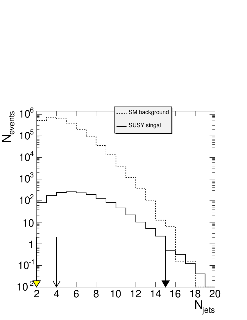
Figure 1: Number of jets with E_T $>$ 40 GeV. Solid lines denote the SUSY signal, while dashed lines - the sum of the SM background distributions. Empty arrow is for classical analysis cut choice, filled colored arrows (black and gray/yellow) are GARCON optimized cuts (values for verification step).

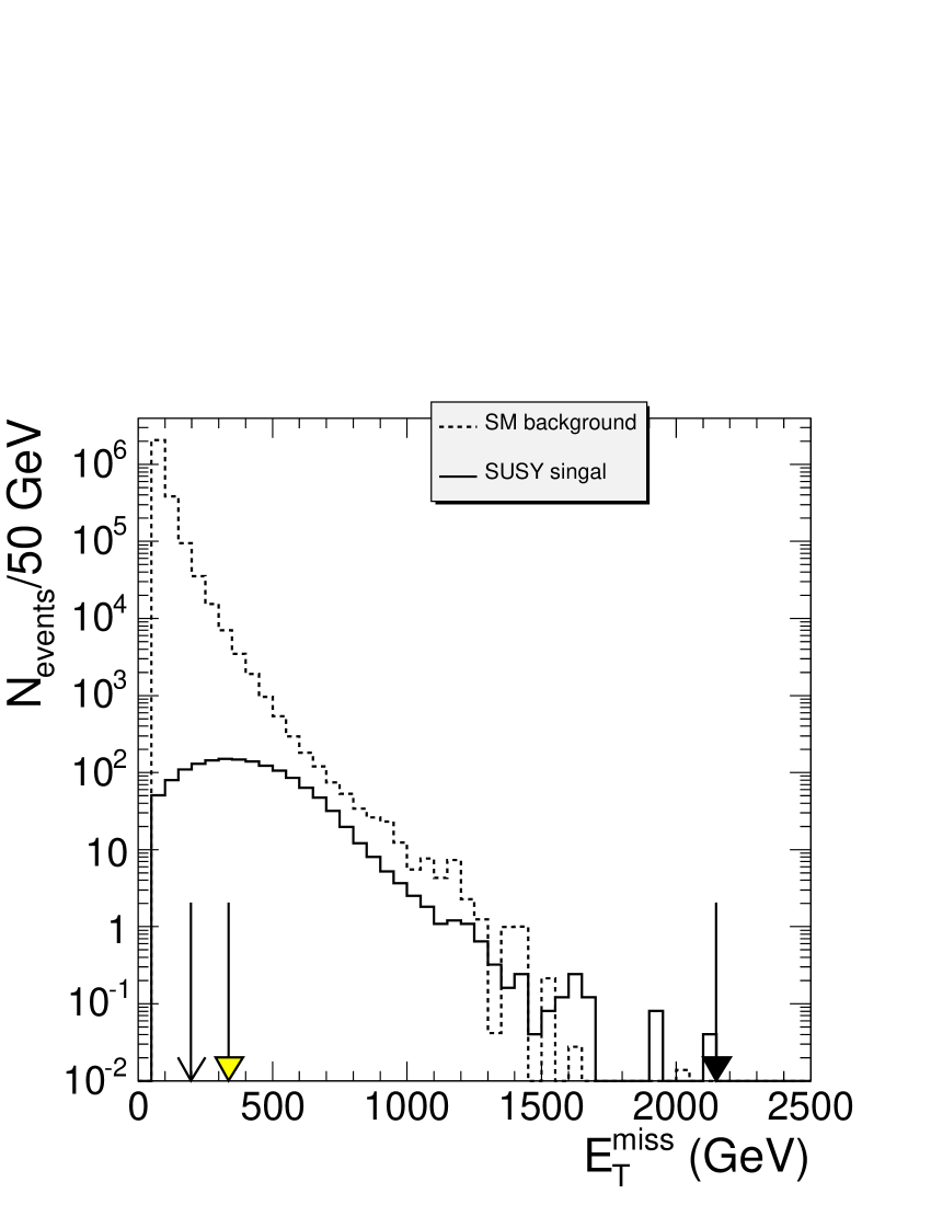
Figure 2: Distribution of missing transverse energy. The same notations as for Fig. 2.

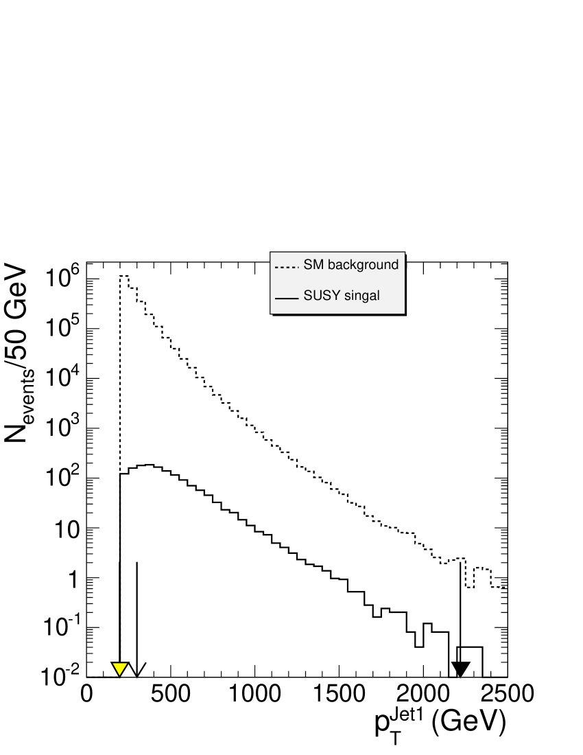
Figure 3: Transverse energy of the hardest-E_T jet. The same notations as for Fig. 2.

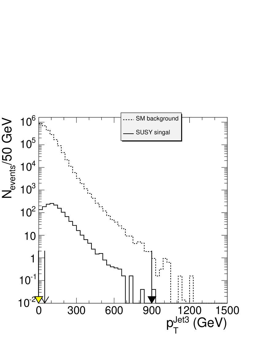
Figure 4: Transverse energy of the third-hardest-E_T jet. The same notations as for Fig. 2.

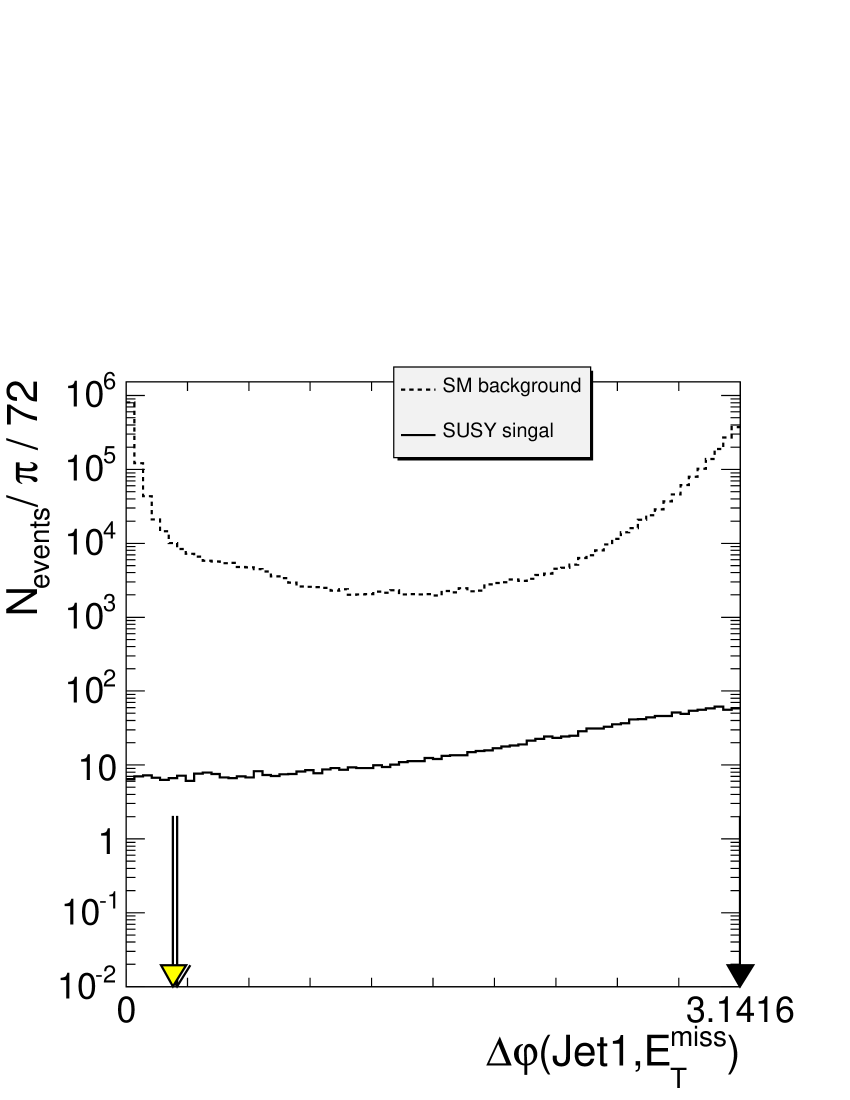
Figure 5: Azimital angle distance between leading jet and transverse missing energy. The same notations as for Fig. 2.

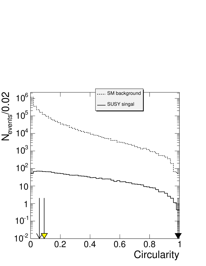
Figure 6: Distribution of the circularity. The same notations as for Fig. 2.

4 GARCON Analysis

4.1 Evolution algorithms

GARCON, GA-based programs in general, exploits evolution-kind algorithms and uses evolution-like terms:

• Individual - is a set of qualities, which are to be optimized in a particular environment or set of requirements. In HEP analysis case, an Individual is a set of lower and upper rectangular cut values for each of variables under study/optimization.

• Environment or set of requirements of evolutionary process in HEP analysis case is a Quality Function (QF) used for optimization of individuals. Significance of a signal over background is another widely used term in HEP community for QF. The higher QF value the better is an Individual. For a HEP analysis Quality Function may be as simple as $S/\sqrt{B}$, where S is a number of signal events and B is a total number of background events after cuts, or almost of any degree of complexity, including systematic uncertainties on different backgrounds, etc .

• A given number of individuals constitute a Community, which is involved in evolution process.

• Each individual involved in the evolution, i.e. in breeding with a possibility of mutation of new individuals, death, etc. The higher is the QF of a particular individual, the more chances this individual has to participate in breeding of new individuals and the longer it lives (participates in more breeding cycles, etc.), thus improving community as a whole.

• Breeding in HEP analysis example is a producing of a new individual with qualities taken in a defined way from two “parent” individuals.

• Death of an individual happens, when it passes over an age limit for it’s quality: the bigger it’s quality, the longer it lives.

• Cataclysmic Updates may happen in evolution after a long period of stagnation in evolution, at this time the whole community gets renewed and gets another chance to evolve to even better quality level. In HEP analysis case it corresponds to a chance to find another local and ultimately a global maximum in terms of quality function. Obviously, the more complicated phase space of cut variables is used, the more chances exist that there are several local maximums in quality function optimization.

• There are some other algorithms involved into GAs. For example mutation of a new individual. In this case, “new-born” individual has not just qualities of its “parents”, but also some variations, which in terms of HEP analysis example helps evolution to find a global maximum, with less chances to fall into a local one. There are also random creation mechanisms serving the same purpose, etc.

4.2 Input for GARCON

GARCON uses the same input information as a classical analysis: arrays of variable values, see Appen. A, the same what is needed to perform a classical eye-balling cut optimization.

Details on chosen variables are given in Sec. 2.2.

4.3 Optimization

Each cycle/“year” of evolution includes a community update, that is breeding process, possible mutation of new individuals, quality and age calculations for each individuals, death of worst and too old individuals, etc.

As described above the better is an individual QF, the longer it lives and hence the more chances it has to produce new individs, improving quality of a community as a whole and the very best individ quality as a final goal. This very best individ or the very best set of min/max cut variable values, which corresponds to the best achievable quality function (significance of signal over background) is a final goal and final output of the GARCON optimization step: rectangular cut values recommended by the optimization procedure.

Figures 8, 8, 10 and 10 show dynamics/evolution of the $S_{c12}$ quality function, dynamics on MET and circularity cut variable values and amount of time used for optimization.

Typical optimization procedure with GARCON takes from a few seconds to several hours depending on the amount of statistics and additional requirements like minimal number of events to survive after all cuts, etc. As one can see from Fig. 10 results close to the best are already achieved before the first cataclysmic update, which happend at year $<50$ and required less than 3.5 hours of CPU time for 10 variables (Sec. 2.2) or 20 optimized parameters with precision on each 2.5% and about $4\cdot 10^{5}$ generated events on input (after pre-selection, see Sec. 2.2).

Optimized values for all the cut parameters are listed in Table 2. Results in terms of chosen significance estimator as well as signal to background number of events ratio, final event numbers are listed in Tab. 3. Cuts are also illustrated on cut parameter distribution in Figs. 2-6.

Table 2: Min and max values for cut parameters. Cut values for the classical analysis are the same. Cut values for GARCON verification are rounded off in comparison to those we have from optimization to reflect resolution effects and possible lower/upper limits.

cut parameter	classical	GARCON optimization	GARCON verification
$N_{mu}$	0-inf	0-5	0-5
$p^{1}_{\rm T}$, GeV	0-inf	0-1020	0-inf
$ISOL^{1}_{mu}$, GeV	0-inf	0-1080	0-inf
$N_{j}$	4-16	2-16	2-16
$E^{1}_{\rm T}$, GeV	300-inf	200-2220	200-inf
$E^{3}_{\rm T}$, GeV	50-inf	0-901	0-inf
E${}_{\rm T}^{miss}$, GeV	200-inf	342-2150	340-inf
$\Delta\phi(\mu^{1},E_{\rm T}^{miss})$, rad	0- $\pi$	0.297-$\pi$	0.297-$\pi$
$\Delta\phi(jet^{1},E_{\rm T}^{miss})$, rad	0.262-$\pi$	0.245-$\pi$	0.245-$\pi$
circularity	0.06-1	0.0924-0.993	0.0924-1

Analysing cut values and their distributions (Figs. 2-6) one can see that some variables after GARCON optimization converge to the limits of a particular distribution. From the technical point of view the reason for this is because GARCON works only with input values and doesn’t have plus or minus infinity e.g. at its disposal. From the practical point of view, it means that min or max cut on a particular variable or the whole variable is not useful in comparison to other variables in terms of improving signal to background significance and GARCON shows it. As an example we can consider $E^{1}_{\rm T}$ and $E^{3}_{\rm T}$ before and after all cuts (except the cut on $E^{1}_{\rm T}$ or $E^{3}_{\rm T}$ correspondingly), the examples of variables for which GARCON and classical cut values are different: compare Figs. 4 and 4 for distributions before and Figs. 12 and 12 - after the cuts applied.

4.4 Verification

As mentioned earliler, the available MC statistics was divided in two parts. The second part is used for a “blind” analysis or results stability verification.

After we got the cut values from optimization step, we round them off to the level of expected precision  for each parameter (see Tab. 2) and apply them to the second half of the statistics.

Results are shown in Tab. 3. One can see that results are stable.

Table 3: Final results comparison for classical and GARCON (for optimization and verification steps) approaches in terms of $S_{c12}$ and $S_{cL}$ significance estimators as well as ratio of final number of signal to total background events and those numbers of events with MC statistical error included.

parameter	classical optimization	classical verification	GARCON optimization	GARCON verification
$S_{c12}$	8.1	8.0	15.3	14.7
$S_{cL}$	8.1	8.1	15.8	15.2
S/B	0.102	0.102	0.506	0.469
$N_{signal}$	665 $\pm$ 7	663 $\pm$ 7	574 $\pm$ 7	567 $\pm$ 7
$N_{background}$	6496 $\pm$ 160	6503 $\pm$ 160	1130 $\pm$ 121	1210 $\pm$ 121

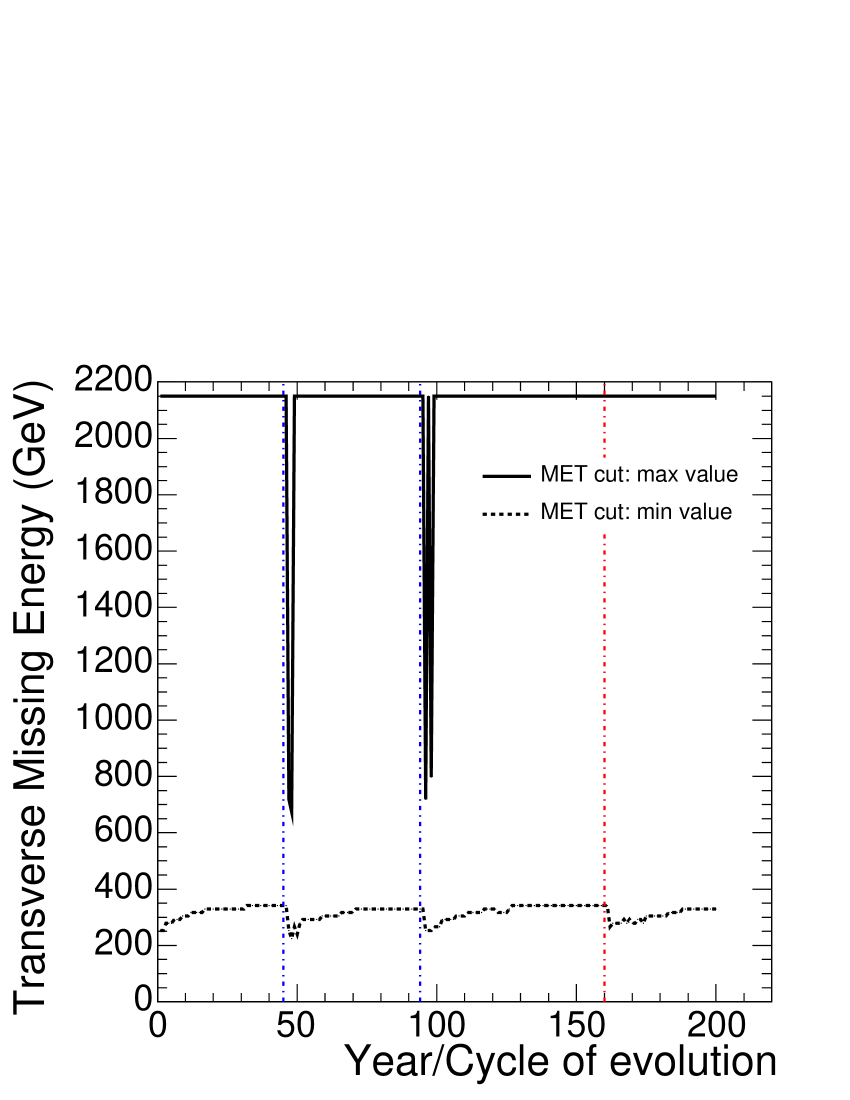
Figure 7: Evolution of the cuts on MET. Upper and lower curves are for min and max cut values on the variable. Vertical dotted-dashed lines show cataclysmic update times, the right one corresponds to a cataclysmic update after the best result achieved.

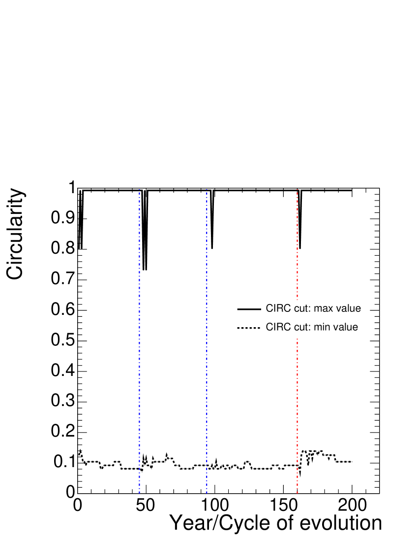
Figure 8: Evolution of the cuts on CIRC. Notations are the same as for Fig. 8.

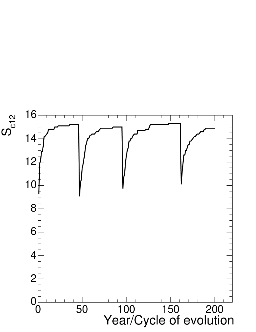
Figure 9: Significance ($S_{c12}$) estimator value dynamics. Notations are the same as for Fig. 8.

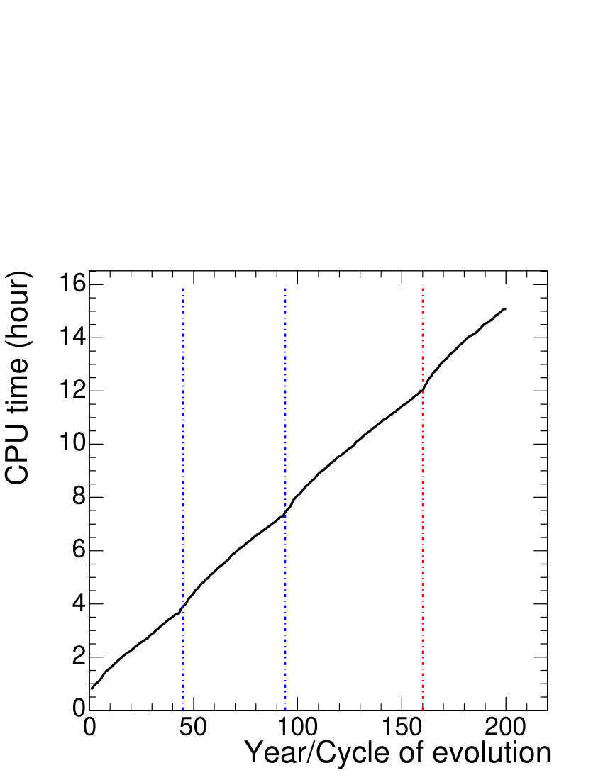
Figure 10: Amount of time spent for evolution. Notations are the same as for Fig. 8.

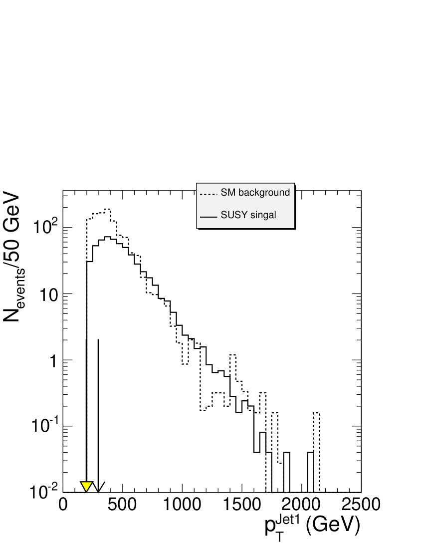
Figure 11: Transverse energy of the hardest-E_T jet. The same notations as for Fig. 2.

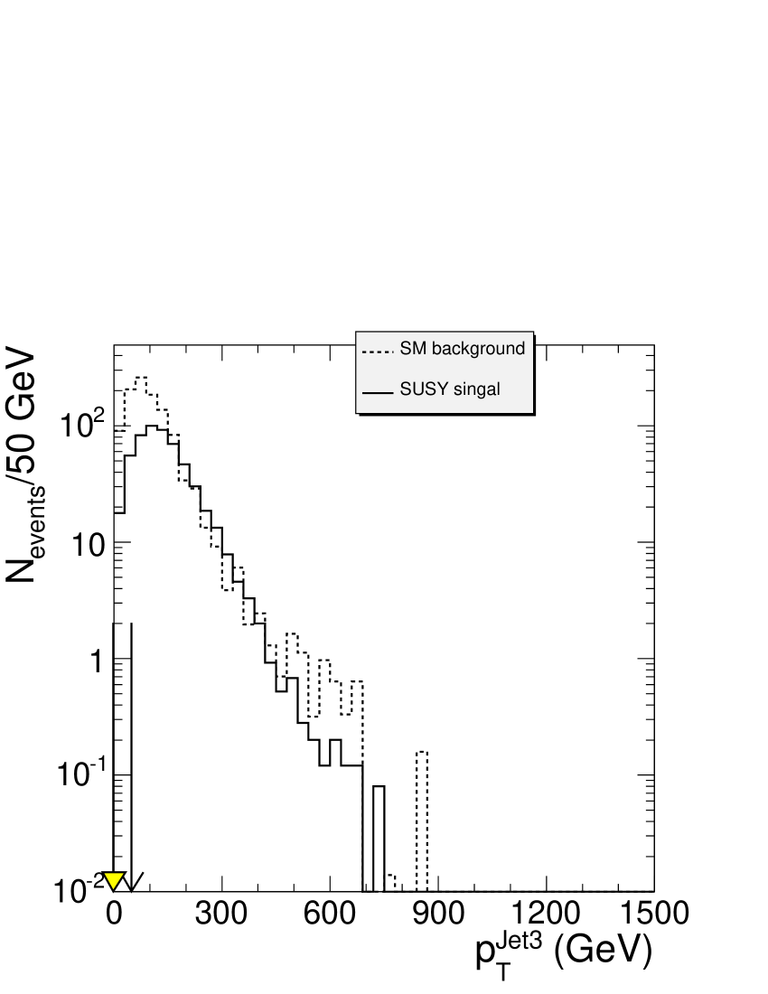
Figure 12: Transverse energy of the third-hardest-E_T jet. The same notations as for Fig. 2.

4.5 Comparison between classical and GARCON approaches

Difference in performance in terms of significance (8 vs. 15) and signal to background events number ratio (0.1 vs. 0.5) may not be a typical gain when GARCON is used vs. a classical approach: classical approach may be pretty sophisticated (as well as time dedicated to it may be large). What is important to emphasize is that GARCON does optimization and verification of results stability in an automatic manner, not requiring any special treatment of either input data or output results and does converge to virtually the best set of cuts in typically hours time.

Different cases which show GARCON usage in much more complicated analyses cases can be found elsewhere [7, 8, 9].

5 GARCON v2.0: User’s Manual.

5.1 Introduction

This is a user’s manual on how to run GARCON, GA program v2.0 and use its output in physics analyses. The program is designed for rectangular cuts optimization (with same interpretation and usage of cut values as you would expect from classical, eye-balling rectangular cut values selection).

You may find useful the following presentations linked to the GARCON home page [5]:

• “GARCON - Genetic Algorithm for Rectangular Cuts OptimizatioN” - this is a how-to use the program talk

• “Genetic Algorithm studies and comparisons using different significance estimators”

• “Genetic Algorithm and example application in a SUSY search”

5.2 Installation

For now to make user’s and developers life easier code is available as a static library pre-compiled at Scientific Linux PCs (CERN’s Linux Red Hat 9.0 version) it has a template for a user to define optimization function (several widely-used functions described below are also available). All you need is to get an archive from the following web-page (look for “Code” link there) and do:

• go to: http://drozdets.home.cern.ch/drozdets/home/genetic/

• download the most recent version of the program ( garcon-2_0.tar.gz),

• do ’tar -xzf garcon-2_0.tar.gz’ in any directory you would like to work with GA,

• read and follow README file instructions on how to build executable and run GARCON.

You will find there the following files/directories:

• lib/libgenetic.a - is a GARCON library file.

• quality.cc - C++ template file for you to define your own quality/significance function for optimization. (Look inside this file, it has two examples of user’s functions with detailed comments: simple and detailed ones. You should be able to easily construct your own function in a similar way.)

• Makefile - for making binary file: garcon-ga.

• data/ - a directory, where you can store your input data files (see example of their format below).

• dataFiles.dat, initialization.dat, verification.dat, dataErrors.dat, variablesON_OFF.dat - files with input parameters (description is given below).

5.3 How to run GA.

Just use ’./garcon-ga $>$ output.txt’ after you have prepared an executable following instructions in README file and put appropriate parameters into dataFiles.dat, initialization.dat, verification.dat, dataErrors.dat files.

5.4 Input data sample files format.

Example is in: data/example.dat, see also Appen. A. NOTE: This file is just an example of format, it is a shortened version of a real data file.

First line is for a process name (one word). In example it is: lm1.

Second line is for weight per event in sample (usually weight calculated as: $weight=\frac{\sigma\int L\epsilon}{N_{events-in-sample}}$). Do not forget to correspondingly increase weights when you divide your statistics into two parts, one for optimization and one for verification steps. In example it is: 0.324 One can also vary weight with weightCoef parameter described in Sec. 5.6.

Third line is for variable/cut names (one word for each). In the example file there are 12 of them: met njet et_jet1 et_jet2 eta_lep1 eta_lep2 deltaR cosTheta dphi_l1met dphi_j1met njet30 njet50.

Forth and the following lines are for input data. Values of the above listed variables for each event for a particular process. (One input file per process! One line per event!) See example in the file.

5.5 Input parameters. File dataFiles.dat.

This file in each line has a PATH to a particular input data sample. The paths may be relative (relative with respect to the directory where you run GA) or absolute (always works).

Example is in: dataFiles.dat release file version.

NOTE: input file for signal is always the last one!

You will need two such files with two lists of input files if you are to perform optimization of cuts and verification of results stability.

5.6 Input parameters. File initialization.dat.

This file has input parameters for GA, see Appen. B.

• internal, 0 - three first service parameters. Just put them 0, they are not used in the public version and exist for debugging purposes.

• Integer maxNumberFeatures - the number of cut parameters used in your analyses (with values provided in input files of course). It equals to 12 in the described above input data sample files format example.

• Integer maxNumberProcesses - should be equal to number of input files. It equals to 9 for the dataFiles.dat release file version.

• Integer maxNumberFeatureValues - this says to GA how precise you want your cuts, how small step to use. For example if you put maxNumberFeatureValues equal 40, it means that cut step corresponds to 2.5% (100/40) of events cut every other cut value. (Signal distributions are used to define cut values. Steps are not equal, they depend on events density for each distribution.)

• Integer initNumberPopulation, greater than 1 - this would be the number of different cut sets (Individuals) involved in evolution. Better to avoid settings too small ($<<30$) or too big ($>>500$). Default value of 100 is a reasonable choice.

• Integer maxNumberBestIndivids, greater than 0 and smaller than initNumberPopulation - should be much smaller than initNumberPopulation. This is the number of the best cut sets. These are cut sets which get priority in GA iteration steps. (There is always one the very best cut set which is printed in all the details.) Default is 5 (for 100 initNumberPopulation).

• Integer ageLimit, greater than 0 and smaller than yearsForEvolution - how long each cut set (Individual) will be involved in evolution iterations. ageLimit is also the limit of how long the very best cut set may not change before the whole population of cut sets will be forced to get new try (cataclysmic update). (This “new try” or critical update allows GA to try to find another maximum in case there are more than one local max for significance in a given parameter space.) Values between 10-50 are good to try. Default is 10.

• Real mutationFactor, from 0 to 1 - technical. Shows a degree of randomness in mutation process. Default is 0.8. Values between 0.01 and 1.00 can be tried.

• Integer yearsForEvolution, greater than 0 (less than 1000) - number of iteration cycles for the whole optimization. Several hundred are OK. (This number should be several times bigger than ageLimit.)

• Integer optimFlag, 1 or 0 - 1, if you do optimization, 0 if you perform verification of results. First is to be performed on one part of the statistics you have in analysis and is for finding the best cuts set. The second is to verify stability of the results using output from the optimization step.

• Integer SignificanceChoice, 0, 1, 2, 3, 4, 5 or 6:

  • 0 is for $S_{1}=S/\sqrt{B}$,

  • 1 is for $S_{2}=S/\sqrt{S+B}$,

  • 2 is for $S_{c12}=2\cdot(\sqrt{B+S}-\sqrt{B})$,

  • 3 is for $S_{cL}=\sqrt{2\cdot(S+B)\cdot log(1.0+S/B)-2\cdot S}$,

  • 4 is for $S/B$, where B - is a number of all the background events after cuts, and S - is a number of signal events after cuts,

  • 5 and 6 are for user defined significance functions (5 is for a simple one and 6 allows user to access details for each event, see Appen. C).

  Look at the “Genetic Algorithm studies and comparisons using different significance estimators” talk for a hint on a particular significance estimator stability and differences between them.

• Real minEventsCoefficientSignal and minEventsCoefficientBackground - minimal number of events, which should survive after cuts, for background processes calculated as $minEventsCoefficientBackground\cdot\sqrt{\sum_{i=1}^{Nbackground-processes}weight_{i}^{2}}$ and $minEventsCoefficientSignal\cdot weight_{signal}$ for signal process. Default is 5. This parameter or final events number thresholds affect results stability as they do in a classical approach as well.

• Real weightCoef - a re-weighting coefficient. For example if you have your samples prepared for 10$fb^{-1}$ and would like to see how results of optimization would change for other luminosities, for example for 100$fb^{-1}$, you can simply put weightCoef = 10. This parameter is also useful when you divide your statistics to two parts for optimization and verification and don’t want to remember to change weights in all the data samples, you may just change weightCoef (if you divide statistics half-by-half, you need to multiply weight for every sample by 2, or put weightCoef=2 to have calculations done for the same integrated luminosity).

  Example is in: initialization.dat release file version.

5.7 Input parameters for verification. File verification.dat.

First line is for number of cut sets to be verified. In example it is 4, see Appen. D.

Each of the best cut sets is listed in an output file after optimization step. The very best one for each iteration is printed in all details with cut values, and there are some details on maxNumberBestIndivids of best cut sets (cut values, age, etc).

So, you may use the following procedure after optimization step is done. Do: ’grep Calculated output.txt’, you will get a list of the best values of significances. You will likely see that there were several attempts by GA to find the best optimization (significance/quality increases, then stays stable, then starts over again). So, you may find out looking at the output file what cut sets (’Min Individ Feature Values’ and ’Max Individ Feature Values’ - upper and lower cut values) corresponds to a few maximums you find in the ’grep Calculated output.txt’ listing. Just cut and paste them into verification.dat (two lines per cut set: ’Min Individ Feature Values’ and ’Max Individ Feature Values’). There are four such pairs in example file.

Then run GA again, but with optimFlag set to 0. Better to do this on a different part of the statistics (“blind” experiment) and with cut parameter values rounded off to levels of corresponding precisions to avoid cuts “overtuning”.

5.8 Input parameters. File dataErrors.dat.

This file has a line of “penalty/priority” factors for each process in order as they are listed in dataFiles.dat, see Appen. E.

Example is in: dataErrors.dat release file version.

NOTE: input file for signal is always the last one!

The idea of the “penalty/priority” factors is to apply a simple estimation on systematic effects influences (alternative possibility is to define a sophisticated user QF, see Sec. 5.6 and Appen. C). If the factor values are different from 0.0, then equations for Significance Functions described above will be calculated with modified number of signal and background events: $S\rightarrow S+kS\cdot S$, $B=\sum{B_{i}}\rightarrow B=\sum(B_{i}+kB_{i}\cdot B_{i})$, where $kS$ and $kB_{i}$ are introduced in dataErrors.dat factors.

HINT: putting a factor equal to -1.0 will effectively switch off a particular process. (-1.0 is the minimal value for a factor, upper value is not limited.)

HINT: putting $kB_{i}>=0$ and $kS<=0$ will provide you with a conservative estimation (opposite signs - with optimistic values of Significance).

HINT: one may try these factors after optimization, during “verification step”, getting a feeling of different scenarios.

5.9 Input parameters. File variablesON_OFF.dat.

This file has a line of ON/OFF switches for each parameter in input files in order as they are listed in input data files, see Appen. F. This allows user to prepare input data files with exhaustive list of possible cut parameters and then perform optimization studies on different combinations of the parameters.

5.10 How to use GA results.

Basically cut sets (pairs of ’Min Individ Feature Values’ and ’Max Individ Feature Values’) for each particular cut/parameter are similar in use and interpretation as classical, eye-balling cuts one usually looking for to discriminate between signal and background event. So, once you’ve got GA results and verified their stability you may go on with your analysis as after you find out a set of classical rectangular cuts for your distributions.

HINT: the very best result is repeated at the end of the output.

HINT: output contains details on dynamics of all the significance estimators available (while performing optimization on one of them).

HINT: you may want to use not the very best Individual (cuts set), but for example a one corresponding to a local maximum with worse performance, but better stability. As described above (Sec. 5.6) one of the means of making results stable is to ask for a particular number of events to survive. Obviously, if weight per generated event for a particular process is something like 1000 expected “real” events and cuts kill all the events in MC sample, one effectively has $0\pm 1000$ events expected, which (sero survived events) may be a statistically unstable result.

6 Summary

We presented GARCON program, illustrated its functionality on a simple HEP analysis example, much more complicated examples described for example in the CMS Physics Technical Design Report. The program automatically performs rectangular cuts optimization and verification for stability in a multi-dimensional phase space.

All-in-all it is a simple yet powerful ready-to-use publicly available tool with flexible and transparent optimization and verification parameters setup.

7 Acknowledgments

We would like to thank A. Giammanco, A. Korytov and A. Sherstnev for useful discussions.

Appendix A Input data file format.

A part of one input data example file is given below.

lm1
0.324
met njet et_jet1 et_jet2 eta_lep1 eta_lep2 deltaR cosTheta dphi_l1met dphi_j1met njet30 njet50
383.926 2 550.591 150.944 -0.800319 -1.32351 0.864812 0.86366  0.191271 2.90746 2 2
229.268 3 248.019 103.515 0.930838  -1.82199 3.82118 -0.883346 0.772977 2.64147 2 2
149.199 6 374.811 142.887 -1.5395   -1.73921 1.44724  0.876463 2.00948 1.74833 5 3
266.147 5 369.581 131.862 1.49267    1.98226 0.950259 0.949556 0.6018 2.96775 3 2
360.203 3 242.108 158.631 -1.63074  -1.54017 2.37681  0.733466 2.4858  2.4815 2 2

Appendix B Initialization data format.

An example of initialization input parameters file.

internal 0
internal 0
internal 0
maxNumberFeatures 12
maxNumberProcesses 9
maxNumberFeatureValues 40
initNumberPopulation 100
maxNumberBestIndivids 5
ageLimit 10
mutationFactor 0.8
yearsForEvolution 400
optimFlag 1
SignificanceChoice 3
minEventsCoefficientSignal 5.0
minEventsCoefficientBackground 5.0
weightCoef 1.0

Appendix C User defined significance function.

The whole text of the template is shown below.

#include <iostream>
#include <vector>

using namespace std;

double UserDefinedQuality(const double S, const double B)
{
  // simple example of re-defined S1=S/sqrt(B)
  // using total number of weighted signal (S)
  // and sum of background (B) events

  return S/sqrt(B+0.00001);
}




double UserDefinedQuality(const double S,
                          const double B,
                          const double dS,
                          const double dB,
                          const vector<double> expEvents,
                          const vector<double> dexpEvents,
                          const vector<int> genEvents,
                          const vector<double> weights
                          )
{
  // Detailed User’s Qualty function
  // available variables are:
  // S - total number of weighted signal events
  // dS - MC stat. error on total number of weighted signal events
  // B - total number of sum of weighted background events
  // dB - MC stat. error on total number of sum of weighted background events
  // expEvents - vector with weighted events (signal is the last element)
  // dexpEvents - vector with MC stat. error on weighted events (signal is the last element)
  // genEvents - corresponding numbers of generated events
  // weights - vector of weights per generated event

  // access example is demonstrated below
  if (0)
    {
      cout << "\n\nSignal events: " << S << " +- " << dS << endl;
      cout << "Background events: " << B << " +- " << dB << endl;
      for (int i=0; i<int(expEvents.size())-1; i++)
        {
          cout << "Background Process " << i
               << "\nWeighted background events " << expEvents[i]
               << " +- " << dexpEvents[i]
               << " corresponding to " << genEvents[i] << " gen. events"
               << " with weight " << weights[i]
               << endl;
        }
      int sig_index = expEvents.size()-1;
      cout << "Signal Process:"
           << "\nWeighted events " << expEvents[sig_index]
           << " +- " << dexpEvents[sig_index]
           << " corresponding to " << genEvents[sig_index] << " gen. events"
           << " with weight " << weights[sig_index]
           << endl;
    }


  // simple example
  return S/sqrt(expEvents[0]+0.0000001);
}

Appendix D Verification data format.

An example of verification data format with four different cut sets to try (to verify).

4
165  3  22.2 65.5 -2.48 -2.45 0    -1 0    0    3  2
1470 11 2120 1160  2.48  2.45 4.78  1 3.14 3.14 10 8
224   3 62.8 65.5 -2.49 -2.45 0  -0.821 0   0.476 3  2
1470 11  577 1160  2.48  2.47 4.78  1 3.14 3.14 10 8
224   3 62.8 65.5 -2.49 -2.45 0  -0.821 0.494 0 3 2
1470 11 510  1160  2.49 2.47  2.98 1 3.14 3.07 10 8
150   2 22.2 65.5 -2.48 -2.45 0   -1 0    0.476 2 1
1470 11 2120 378   2.48 2.47  4.78 1 3.14 3.14 10 8

Appendix E Penalty factors.

An example of a “penalty” parameters input file. In this example the last sample, signal, gets -0.1 penalty, which means 10% reduction in the number of signal events.

0.0 0.0 0.0 0.0 0.0 0.0 0.0 0.0 -0.1

Appendix F Switching variables ON/OFF file format, data errors file format.

An example of switching variables ON/OFF file format. In this example 3rd and 11th variables are switched off from the analysis.

1 1 0 1 1 1 1 1 1 1 0 1

References

-
[1]
R.K. Bock, W. KRISCHER, “The Data Analysis
BriefBook”, http://rkb.home.cern.ch/rkb/titleA.html
Wikipedia, the free encyclopedia, “Genetic algorithm”, http://en.wikipedia.org/wiki/Genetic_algorithm
an overview: D. Beasley, D.R. Bull, and R.R. Martin, “An Overview of Genetic Algorithms”, University Computing 15(2) (1993) 58 - [2] John H. Holland. Adaptation in natural and artificial systems. The University of Michigan Press, Ann Arbor, 1975.
- [3] David E. Goldberg. Genetic algorithms in search, optimization and machine learning. Addison Wesley, 1989.
-
[4]