Abstract

In the minimal Universal Extra Dimension (mUED) model, there are four physical scalar particles at the $n=1$ level, two charged and two neutral. Due to the almost degenerate nature of the spectrum, the detection of these scalars is a major challenge, perhaps the greatest experimental challenge if UED-type new physics is observed at the Large Hadron Collider (LHC). We explore the possibility of detecting these particles at the International Linear Collider (ILC), and emphasise the need of having an excellent soft $\tau$ detection efficiency.

PACS numbers:  11.25.Mj, 14.80.Cp, 13.66.Fg
Keywords:  Universal Extra Dimension, Electron-Positron Collider, Excited Higgs Bosons

I Introduction

The possibility of a compactified extra dimension was first discussed by Nordström, Kaluza and Klein [1] . Such extra dimension (ED) models were later revived by the necessity of a consistent formulation of string theories [2]. Of course, even without string theories, the world may have one or more compactified dimensions. There are a number of such ED models, and they differ mainly in two ways: first, the number of EDs, the geometry of space-time, and the compactification manifold, and second, which particles can go into the extra dimensions (hereafter called bulk) and which cannot.

In the so-called Universal Extra Dimension (UED) model proposed by Appelquist, Cheng, and Dobrescu [3], all SM particles can go into the bulk. In the simplest UED scenario, there is only one extra dimension, denoted by $y$, compactified on a circle ($S_{1}$) of radius $R$. The model predictions remain essentially unchanged if there are more extra dimensions, with a hierarchical radii of compactification. We will focus on the simplest scenario only.

To get chiral fermions at low-energy, one must impose a further ${\cal Z}_{2}$ symmetry ($y\leftrightarrow-y$), so that finally we have an $S_{1}/{\cal Z}_{2}$ orbifold. As is well-known, a higher dimension theory is nonrenormalizable and should be treated in the spirit of an effective theory valid upto a scale $\Lambda>R^{-1}$. All fields have five space-time components; when brought down to four dimensions, for each low-mass (zero-mode) Standard Model (SM) particle of mass $m_{0}$, we get an associated Kaluza-Klein (KK) tower, the $n$-th level (this $n$ is the KK number of the particle) of which has a mass given by

$$m_{n}^{2}=m_{0}^{2}+\frac{n^{2}}{R^{2}}.$$ (1)

This is a tree-level relationship and gets modified once we take into account the radiative corrections.

Another important feature of the UED scenario is the conservation of the KK number. This is simply a reflection of the fact that all particles can go into the fifth dimension and so the momentum along the fifth dimension must be conserved. Also, this means that the lowest-mass $n=1$ particle, which turns out to be the $n=1$ photon, is absolutely stable. Such a lightest KK particle (LKP), just like the lightest supersymmetric particle (LSP), is an excellent candidate for dark matter [4, 5, 6, 7, 8]. In fact, existence of such a dark matter candidate is a general property of any theory with such a ${\cal Z}_{2}$ symmetry. To us, this seems to be the greatest theoretical motivation for UED-type models.

Radiative corrections to the masses of the KK particles have been computed in [9, 10, 11]. These papers, in particular [10], show that the almost mass-degenerate spectrum for any KK level, resulting from eq. (1), splits up due to such correction terms. There are two types of correction, arising from the fact the fifth dimension is inherently different from the four large dimensions (a breaking of the Lorentz invariance). The first one, which results just from the compactification of the extra dimension, is in general small (zero for fermions) and is constant for all $n$ levels. This we will call the bulk correction, which arises when the loops can sense the compactification (e.g., loops with nonzero winding number around $y$). The second one, which we will call boundary correction, is comparatively large (goes as $\ln\Lambda^{2}$ and hence, in principle, can be divergent), and plays the major role in determining the exact spectrum and possible decay modes. The boundary correction terms are related with the interactions present only at the fixed points $y=0$ and $y=\pi R$. If the interaction is symmetric under the exchange of these fixed points (this is another ${\cal Z}_{2}$ symmetry, but not the ${\cal Z}_{2}$ of $y\leftrightarrow-y$), the conservation of KK number breaks down to the conservation of KK parity, defined as $(-1)^{n}$. Thus, LKP is still stable, but one can in principle have KK-number violating vertices in the theory, where the violation is by an even amount. For example, it is possible to produce an $n=2$ state from two $n=0$ states.

The role of linear colliders in precision study of TeV-scale extra dimension models has been already emphasized in the literature [12]. The low-energy phenomenology has been discussed in [3, 13, 14, 15, 16, 17, 18, 19], and the high-energy collider signatures in [20, 21, 22, 23, 24, 25, 26, 27, 28]. The limit on $1/R$ from precision data is about 250-300 GeV, while the limit estimated from dark matter search [4] is about a factor of two higher. The loop corrections are quite insensitive to the precise values of the radiative corrections. With the proposed reach of the International Linear Collider (ILC) in mind, we will be interested in the range 300 GeV $<R^{-1}<$ 500 GeV.

It was first pointed out in [25] that the signals of the UED models may mimic those of R-parity conserving supersymmetry (SUSY), mainly because of the ${\cal Z}_{2}$ symmetry of both the theories that predicts a missing energy signal once a sparticle or a KK excitation is produced. The decay patterns of excited fermions and sfermions are also similar for a significant part of the SUSY parameter space. One may hope to discriminate these two models by measuring the spin of the excited particles [29, 30, 31], or by producing the $n=2$ gauge bosons as $s$-channel resonances [27]. The standard verdict is that the excited states are to be first seen at the Large Hadron Collider (LHC), and a precision study is to be done at the ILC.

One important point that has not been addressed is the production and subsequent decay and detection of the $n=1$ scalars. This is perhaps the most challenging part of a complete determination of the KK spectrum. There are four such excited scalars at the $n=1$ level, two charged and two neutral. Not only they are almost mass degenerate, it appears from a study of the spectrum that their only possible decay channel is to the $n=1$ $\tau$ leptons. Ultimately, what we will be left with are 2-4 soft $\tau$ leptons plus a huge amount of missing energy. These $\tau$s may be so soft as to avoid detection. Thus, if we are unlucky, the whole excited scalar sector may be invisible! This is to be compared with the SUSY models, where one is almost certain to detect some of the Higgs bosons if they are produced. A detailed discussion of this follows in Sections 2 and 3.

Even if the soft $\tau$’s are visible (and for most of the parameter space they are), the background is still severe. The most important background comes from another UED process, the $s$-channel production of excited $\tau$-lepton pair, which subsequently decays to a pair of $n=0$ soft $\tau$’s and two LKPs. The signal is indeed a fraction of the background, so we need some luck to detect the signal. There are other backgrounds, but for most of the parameter space they can be brought down by suitable cuts.

The minimal UED model is completely specified by three input parameters: $1/R$, inverse of the compactification radius, $\Lambda$, the effective cutoff of the theory, and ${\bar{m}_{h}}^{2}$, the boundary mass squared (BMS) term for the excited scalars. The last parameter can be determined if we can have a precision study of the excited scalar sector. This appears very tough, if not outright impossible, even at the ILC. However, we will derive a theoretical bound on ${\bar{m}_{h}}^{2}$ from the fact that the $n=1$ charged Higgs boson must not be the LKP. This occurs for large negative values of ${\bar{m}_{h}}^{2}$, of the order of $-(10^{3}$-$10^{4})$ GeV².

The paper is arranged as follows. In Section 2 we discuss, briefly, the salient features of the excited Higgs sector of the minimal UED model. In Section 3, we discuss the important two- and three-body production processes involving one or more excited scalars, and show their subsequent decay chains. We also estimate their production cross-section as a function of $1/R$, $\Lambda$ and ${\bar{m}_{h}}^{2}$. This gives us an idea of the parameter space where such excited bosons can be detected and where they just cannot be. The possible backgrounds are also shown. In Section 4, we find the theoretical lower bound on ${\bar{m}_{h}}^{2}$ from the non-LKP condition. We summarize and conclude in Section 5.

Let us mention here that though the main focus is on the ILC, an identical study may be performed for CLIC, the proposed multi-TeV $e^{+}e^{-}$ machine, with an optimised $\sqrt{s}=3$ TeV (and may be upgraded to 5 TeV), and luminosity of $10^{35}$ cm^-2 s^-1. The electron beam at CLIC may be polarised upto 80%, and the positron beam upto 60-80%, from Compton scattering off a high power laser beam [32]. Clearly, the reach of CLIC will be much higher.

II Scalar Sector of UED

Every field in 5 dimension ($x^{\mu},y$) can be decomposed in terms of even and odd components:

$$\phi_{+}(x^{\mu},y) = \frac{1}{\sqrt{\pi R}}\phi_{+}^{(0)}(x^{\mu})+\frac{\sqrt{2}}{\sqrt{\pi R}}\sum_{n=1}^{\infty}\cos\frac{ny}{R}\phi_{+}^{(n)}(x^{\mu}),$$

$$\phi_{-}(x^{\mu},y) = \frac{\sqrt{2}}{\sqrt{\pi R}}\sum_{n=1}^{\infty}\sin\frac{ny}{R}\phi_{-}^{(n)}(x^{\mu}).$$ (2)

At orbifold fixed points $y=0$ and $y=\pi R$, the odd fields are projected out. Also, any vertex must contain an even number of odd fields to survive under integration over $y$. For the fermions, left-chiral doublets and right-chiral singlets are even, while the opposite combinations are odd. It is clear that the Higgs fields must be even to maintain the proper Yukawa couplings.

In the $n=1$ level, there are four scalar fields: $H^{0}$, $\chi^{0}_{1}$, and $\chi^{\pm}_{1}$ . The superscript refers to the charge whereas the subscript refers to the KK number. The last three fields are just the excitations of the $n=0$ Goldstone bosons. There are three more color-neutral scalars, coming from the fifth components of the gauge fields $W^{\pm}$ and $Z$. They are ${\cal Z}_{2}$-odd fields, and can occur first only at the $n=1$ level. They should mix with the Goldstone excitations, and a combination of them will act as the Goldstone boson of the $n=1$ level. For the neutral fields, this combination, for the $n$-th level, is given by

$$G^{0}_{n}=\frac{1}{m_{Z_{n}}}\left[m_{Z}\chi^{0}_{n}-\frac{n}{R}Z^{5}_{n}\right],$$ (3)

and a similar expression for the charged Goldstones. The orthogonal combinations will remain as the physical scalar fields, and we will call them $A^{0}$, and $H^{\pm}$. It is clear that if $1/R\gg m_{W,Z}$, the Goldstones are esentially the fifth components of the gauge bosons, whereas the physical scalars are the excitations of the $n=0$ Goldstones (and the $n=0$ Higgs boson).

In the absence of radiative corrections, the tree-level masses of the excited scalars are given by

$$m_{H_{n}^{0},A_{n}^{0},H_{n}^{\pm}}^{2}=m_{n}^{2}+m_{h,Z,W^{\pm}}^{2},$$ (4)

but this is modified by radiative corrections, whose effect is simply to add a universal term $\delta m_{H}^{2}$ to the right-hand side of eq. (4) [10]. The radiative correction is given by

$$\delta m_{H}^{2}=m_{n}^{2}\left[\frac{3}{2}g_{2}^{2}+\frac{3}{4}{g^{\prime}}^{2}-\lambda\right]\frac{1}{16\pi^{2}}\ln\frac{\Lambda^{2}}{\mu^{2}}+{\bar{m}_{h}}^{2},$$ (5)

where $g^{\prime}$ and $g_{2}$ are the $U(1)_{Y}$ and $SU(2)_{L}$ gauge couplings respectively, and $\lambda$ is the self-coupling of the Higgs boson, given by $m_{h}^{2}=\lambda v^{2}$ where $v=246$ GeV. $\Lambda$ is the effective cutoff scale and $\mu$ is the regularization scale, which may be taken for our case to be $1/R$. The term ${\bar{m}_{h}}^{2}$ is arbitrary; this is the BMS term for the excited scalars, and is not a priori calculable. Along with $1/R$ and $\Lambda$, ${\bar{m}_{h}}^{2}$ forms the complete set of input parameters to specify the minimal UED model (of course, one needs to know the $n=0$ Higgs boson mass, $m_{h}$). Note that the hierarchy $m_{H^{0}}>m_{A^{0}}>m_{H^{\pm}}$ is fixed.

The necessary Feynman rules are easy to derive; they come from the kinetic term $(D_{M}\Phi)^{\dagger}(D^{M}\Phi)$ of the Higgs field, where $M$ runs over all the five dimensions. After compactification, this generates the couplings of the $n=0$ Higgs boson with a pair of excited gauge bosons, with a pair of the fifth component of the gauge bosons, and, the couplings of the excited Higgs bosons to $n=0$ and excited gauge bosons. As we have said earlier, no vertex can have an odd number of ${\cal Z}_{2}$-odd fields, and Higgs excitations are even, so there is no need to take the fifth components of the gauge fields into account (this can be ensured further by drawing the Feynman diagrams and noting that $n=0$ fields are always ${\cal Z}_{2}$-even).

III Collider Prospects

Before we go on to the production processes, let us see what these excited scalars should decay into. Unless we go to some bizarre corner of the parameter space with inordinately large value of ${\bar{m}_{h}}^{2}$, these scalars are always lighter than $n=1$ quarks, and so cannot decay into them. Similarly, they are also lighter than the excited $W^{\pm}$ and $Z$. The only $n=1$ states that may be below these bosons are the excited leptons (including neutrinos) and $\gamma_{1}$, the LKP. So, almost all the time, they will decay to the excited $\tau$ lepton (remember that KK-number must be conserved).

For large enough values of ${\bar{m}_{h}}^{2}$, all the $n=1$ scalars can be more massive (albeit very slightly) than $W^{\pm}_{1}$. However, we have checked that the splitting is almost never sufficient to have a $n=0$ boson at the final state. A possibility is a three-body decay to a $n=1$ gauge boson and a pair of $n=0$ leptons. With no guarantee of having a soft $\tau$ in the final state, such signals are even more difficult to trace than those we will discuss here.

There are two excited $\tau$ leptons, which we will call $\tau_{1}$ and $\tau_{2}$ (not to be confused with the $n=2$ excitation of $\tau$; we use this notation since we will never talk about $n\geq 2$ excitations in this paper). Both of them are vectorial in nature, but for $\tau_{1}$, the $SU(2)$ singlet, the right-chiral state is even while the left-chiral state is odd under ${\cal Z}_{2}$. For $\tau_{2}$ it is just the opposite . However, all scalars are ${\cal Z}_{2}$-even, and they must decay to $\tau_{1}$ or $\tau_{2}$ accompanied by a $n=0$ $\tau$ (or $\nu_{\tau}$), so ${\cal Z}_{2}$-odd $\tau$s are not produced from $n=1$ Higgs decays.

Thus, a neutral excited scalar will decay to an excited $\tau^{\pm}$ and an $n=0$ $\tau^{\mp}$. The excited $\tau$s will further decay to the ordinary $\tau$ and the LKP. The final result of the cascade is two unlike sign $\tau$ leptons and an LKP. Since the LKP will carry most of the energy (the typical mass difference between LKP and excited scalars is $\sim 10$ GeV), both these $\tau$s will be soft.

What about the chirality of these $\tau$s? (Since they are soft, helicity and chirality can be different.) The coupling of the scalar with the fermions being Yukawa in nature, both right-chiral $\tau_{1}$ and left-chiral $\tau_{2}$ can be produced, accompanied with a $n=0$ $\tau$ of opposite chirality. It can be seen from Table 1 that $\tau_{2}$ is closer to $H^{0}$ and $A^{0}$. So, from kinematic considerations, more $\tau_{1}$s will be produced. It can so happen that the $\tau_{2}$ window is completely closed.

$1/R$	$\Lambda R$	${\bar{m}_{h}}^{2}$	$H^{0}$	$A^{0}$	$H^{\pm}$	LKP	$\tau_{2}$	$\tau_{1}$
300	20	0	325.70	316.22	313.22	301.54	308.95	303.27
300	20	$-$5000	317.93	308.22	305.13	301.54	308.95	303.27
300	20	5000	333.29	324.03	321.10	301.54	308.95	303.27
300	50	0	326.49	317.04	314.04	301.71	311.68	304.28
300	50	$-$5000	318.74	309.05	305.97	301.71	311.68	304.28
300	50	5000	334.06	324.83	321.90	301.71	311.68	304.28
450	20	0	469.77	463.25	461.20	451.07	463.42	454.91
450	20	$-$5000	464.42	457.82	455.75	451.07	463.42	454.91
450	20	5000	475.06	468.62	466.59	451.07	463.42	454.91
450	50	0	471.00	464.50	462.46	451.11	467.52	456.41
450	50	$-$5000	465.66	459.08	457.02	451.11	467.52	456.41
450	50	5000	476.28	469.85	467.83	451.11	467.52	456.41

Table 1: The masses of $n=1$ scalars. Also shown are the mass of the LKP, $\gamma_{1}$, and the masses of the two $n=1$ $\tau$’s (all in GeV). The $n=1$ neutrino is degenerate with $\tau_{2}$. $m_{h}=120$ GeV.

For large negative values of ${\bar{m}_{h}}^{2}$ ($\sim-10^{4}$), $A^{0}$, and even $H^{0}$, can go down below the $\tau_{1}$ threshold. In that case they will be comparatively long-lived, decaying into the LKP plus a fermion-antifermion pair at $n=0$, or simply to a photon and LKP, through a triangle diagram.

The charged boson, $H^{+}$, will decay into a $\tau^{+}$ and a $\nu_{\tau}$. The neutrino, whether $n=0$ or $n=1$, is left-chiral, so the $\tau$ must be right-chiral in nature. The $n=1$ neutrino is unobservable (it decays to a $n=0$ neutrino and the LKP; note that LKP can directly couple to the neutrino since it is almost an excited $B$, the hypercharge gauge boson), and can be called a virtual LKP. Other decay channels are kinematically forbidden (like $H^{+}\to W^{+}\gamma_{1}$) or highly suppressed (like $H^{+}\to\mu_{1}^{+}\nu_{\mu}$), so we will not consider them any further.

For large negative values of ${\bar{m}_{h}}^{2}$, the $\tau$ window may be closed. In that case the only possible decay option is $H^{+}\to{\rm LKP}+f+\bar{f^{\prime}}$ through a virtual $n=0$ $W^{+}$. Since LKP has a very small $W_{1}$-admixture, this decay is bound to have a long lifetime, and may even leave a visible charged track.

In summary, this means that (unless we entertain the possibility of large negative ${\bar{m}_{h}}^{2}$) from pair production of $H^{+}H^{-}$ one gets a pair of unlike sign soft $\tau$s plus missing energy. For the neutral pair $H^{0}A^{0}$ one gets four soft $\tau$s plus missing energy. The problem is that some of these $\tau$s (particularly for the $4\tau$ final state) can be so soft as to miss detection.

In fig. 1 we show the production cross-section for the charged Higgs pair as a function of $1/R$ for $\Lambda R=20$ (the values are not much sensitive on the cutoff). The numerical cumputations were done with the CalcHEP package [33], augmented by the implementation of UED. Figures 2-4 show the cross-section for other rare processes, most of them being hopelessly small, even at ILC (because of backgrounds that are hard to remove, more on this later). $H^{0}$ is mostly produced through the fusion of two vector bosons, one of $n=0$ and the other of $n=1$, associated with two neutrinos or two electrons. As is expected, the cross-sections for those processes that occur via $s$-channel exchanges (like the Bjorken process, $e^{+}e^{-}\to Z_{0}^{\ast}\to Z_{1}H^{0}$) fall with energy, while those from vector boson fusion rise. Thus, the latter may have a better chance at CLIC. There are other channels with tiny contributions, like $e^{+}e^{-}\to Z_{2}\to H^{+}H^{-}$, which we have not included in the analysis. This channel, for example, is tiny even on the $Z_{2}$ resonance and completely negligible off it.

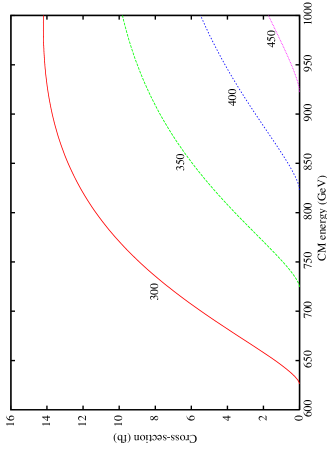
Figure 1: Charged scalar pair production cross-section versus the CM energy for different $1/R$. From top to bottom, the curves are for $R^{-1}=$300, 350, 400, and 450 GeV respectively. $\Lambda R$ has been fixed at 20, but the curves are not sensitive to the precise value of the cutoff.

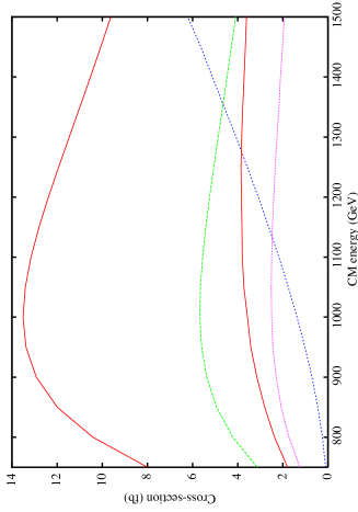
Figure 2: Cross-section of various processes involving one or more excited scalars. The plot is for $1/R=300$ GeV and $\Lambda R=20$. From top to bottom (at the right-hand edge) are the curves for $H^{+}H^{-}$, $H^{0}\nu_{0}\bar{\nu_{1}}$ ($+$ h.c.), $H^{0}A^{0}$, $H^{+}e_{0}\bar{\nu_{1}}$, and $H^{0}A^{0}\gamma$.

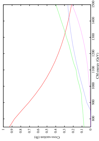
Figure 3: Cross-section of various processes involving one or more excited scalars. The plot is for $1/R=300$ GeV and $\Lambda R=20$. From top to bottom (at the right-hand edge) are the curves for $H^{0}e_{1}^{+}e_{0}^{-}$ ($+$ h.c.), $H^{0}W_{0}^{+}H^{-}$, $W_{1}^{+}H^{-}$ (the falling one) and $Z_{0}W_{1}^{+}H^{-}$ (the rising one).

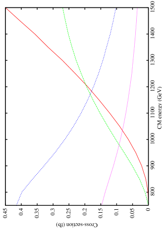
Figure 4: Cross-section of various processes involving one or more excited scalars. The plot is for $1/R=300$ GeV and $\Lambda R=20$. From top to bottom (at the right-hand edge) are the curves for $hW_{1}^{+}H^{-}$, $W_{0}^{+}A^{0}H^{-}$, $Z_{1}H^{0}$, and $H^{0}A^{0}$. $h$ is the SM Higgs boson.

We have also studied four-body processes like $e^{+}e^{-}\to H^{+}H^{-}\nu\bar{\nu},A^{0}A^{0}\nu\bar{\nu},H^{0}H^{0}\nu\bar{\nu}$. These cross-sections are too small even at ILC, and is without any hope of detection. CLIC may do a better job, since these channels, mediated mostly by fusion of $n=1$ vector bosons, rise with $\sqrt{s}$. The first channel may have a cross-section of 14 fb at $\sqrt{s}=3$ TeV.

III.1 SM and UED Backgrounds

The signal process is $e^{+}e^{-}\to n\tau+E\!\!\!/$, where $2\leq n\leq 4$. Remember that these $\tau$s must be soft. For example, with $\sqrt{s}=1$ TeV, $1/R=300$ GeV, $\Lambda R=20$, ${\bar{m}_{h}}^{2}=0$, and $m_{h}=120$ GeV, the maximum energy of the $n=0$ $\tau$s coming from $H^{\pm}$ decay is about 12 GeV. This value is sensitive to the excited scalar-$\tau$ mass splitting, which in turn depends on ${\bar{m}_{h}}^{2}$.

The SM background mostly comes from $W$-pair production, both of which decays to $\tau$ leptons and $\tau$ neutrinos. These leptons are generally hard, and this background can effectively be put under control if we apply an upper energy cut of 12-15 GeV to the $\tau$ leptons. A subdominant background comes from $Z$ pair production, where one of them decays to $\tau^{+}\tau^{-}$ and the other one decays invisibly. Such backgrounds may be eliminated by reconstructing the $Z$. Similar considerations apply for 3-4 $\tau$ signals, where a reconstruction can effectively eliminate such backgrounds.

Another prominent source of SM background is the $\gamma^{*}\gamma^{*}\to\tau^{+}\tau^{-}$ events, where $\gamma^{*}$s originate from the initial electron-positron pair which go undetected down the beam pipe [34]. The $\gamma^{*}\gamma^{*}$ production cross section is $\sim 10^{4}$ pb. About half of these events results in final state $e^{+}e^{-}$ pair as visible particles. The background $\tau^{+}\tau^{-}$ pairs are usually quite soft and coplanar with the beam axis. An acoplanarity cut significantly removes this background. Such a cut, we have checked, does not appreciably reduce our signal. For example, excluding events which deviate from coplanarity within 40 mrad reduces only 7% of the signal cross section. In fact, current designs of ILC envisage very forward detectors to specifically capture the ‘would-be-lost’ $e^{+}e^{-}$ pairs down the beam pipe

The UED backgrounds are more severe. There are at least three two-body processes which can potentially swamp the signal: $e^{+}e^{-}\to W_{1}^{+}W_{1}^{-},\tau_{1}^{+}\tau_{1}^{-}$ and $\tau_{2}^{+}\tau_{2}^{-}$. Among them the $W_{1}$ pair production cross-section is largest [20]: at $1/R=300$ GeV, this is approximately 540 fb for $\sqrt{s}=1$ TeV. Since $W_{1}$ must decay through leptonic channels, the cross-section for getting two $\tau$s plus missing energy in the final state is about 60 fb. This can come from two different subprocesses: $W_{1}\to\tau_{n=1}\bar{\nu_{\tau}}_{n=0}$ and $W_{1}\to\tau_{n=0}\bar{\nu_{\tau}}_{n=1}$ (remember that $n=1$ neutrinos are invisible). Whether one can apply a suitable upper energy cut depends on the precise position of these Higgses, i.e., on ${\bar{m}_{h}}^{2}$. For ${\bar{m}_{h}}^{2}=0$ and $1/R=300$ GeV, the $\tau$s coming from $W_{1}$ can have energies ranging from $2.8$ to 48 GeV. On the other hand, $\tau$s coming from $H^{+}$ are softer, between $2.2$ and $3.3$ GeV. Thus, one can avoid the $W_{1}$-background by putting an upper cut at $3.3$ GeV. This method fails completely if ${\bar{m}_{h}}^{2}$ is large and positive, say $10^{4}$ GeV²; the reason is that $H^{+}$ becomes more massive, almost degenerate with $W_{1}$. Unfortunately, we have no way to guess the value of ${\bar{m}_{h}}^{2}$ beforehand, so even the $W$-background removal is quite difficult.

Similar backgrounds also come from $e^{+}e^{-}\to{\rm LKP}+Z_{1}$ and $e^{+}e^{-}\to 2Z_{1}$. The first one is about five times smaller than the $W_{1}$ pair production rate, but the decay nature of $Z_{1}$ (only to leptons) make the $2\tau+E\!\!\!/$ background about one-fourth as significant as the other. $W_{1}$ and $Z_{1}$ being almost degenerate, the energies of the $\tau$s are going to be similar. A much smaller background comes from $2Z_{1}$ channel.

A more serious background comes from the excited $\tau$ ($\tau_{1}$ or $\tau_{2}$) pair production through $s$-channel photon or $Z$ (unless one sits precisely on the $\gamma_{2}$ or $Z_{2}$ resonances, their contribution can be neglected). The $\tau_{2}$ pair production cross-section is about 100 fb for $1/R=300$ GeV, and slightly less for $\tau_{1}$. (The difference is due to their couplings with $Z$.) It falls with increasing $1/R$, but so does the $H^{\pm}$ production rate. The excited $\tau$s decay only to normal $\tau$s emitting an LKP, so the background is identical to the signal, even in angular distribution. Again, ${\bar{m}_{h}}^{2}$ plays an important role: for ${\bar{m}_{h}}^{2}=0$, $\tau_{2}$ backgrounds can be removed by an identical mechanism to that of $W_{1}$. However, the $\tau_{1}$ background is impossible to remove, or even to reduce significantly. We show, in figures 5 and 6, the possible range of $\tau$ energies coming from $W_{1}$, $\tau_{1}$, $\tau_{2}$, and $H^{+}$, for two values of ${\bar{m}_{h}}^{2}$: 0 and 5000 GeV².

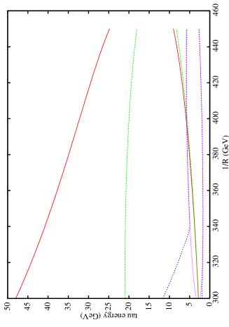
Figure 5: The upper and lower energy bands of $n=0$ $\tau$ lepton coming from $W_{1}$ (solid black), $H^{+}$ (short-dashed blue), $\tau_{2}$ (long-dashed green) and $\tau_{1}$ (dotted magenta) decays. We have set $1/R=300$ GeV, $\Lambda R=20$, ${\bar{m}_{h}}^{2}=0$ and $m_{h}=120$ GeV.

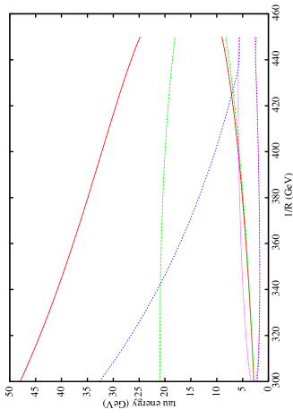
Figure 6: Same as in fig. 5, but for ${\bar{m}_{h}}^{2}=5000$ GeV². All other legends remain the same.

This seems to be almost a no-go: if $W_{1}$ and $\tau_{2}$ backgrounds can be removed, one gets stuck at $\tau_{1}$, or vice versa. For one of the most favorable situations ($1/R=300$ GeV, $\Lambda R=20$, ${\bar{m}_{h}}^{2}=0$, and $m_{h}=120$ GeV), the signal, after providing optimum cuts, is at about $1\sigma$ level, assuming that we know ${\bar{m}_{h}}^{2}$ beforehand, which is an impossibility (unless there is some theoretical model). One way out may be to use the muon channel, $e^{+}e^{-}\to\mu^{+}\mu^{-}+E\!\!\!/$, coming from the production of excited muons only, as a calibration and look for excess events in the $\tau$ channel.

There is also a case where the $\tau$s coming from $n=1$ Higgs decays cannot even be detected. This happens when $m_{H^{+}}$ is close to $m_{\gamma_{1}}$. All the excited scalars will lie close to the LKP, and the $\tau$s will be so soft as to avoid detection. Of course, it may so happen that the $\tau$-window is completely closed for $H^{+}$, which should then decay to $\mu^{+}$ with a much longer lifetime.

Thus, there are three levels of challenge. First, to have a theoretical prediction for ${\bar{m}_{h}}^{2}$, perhaps from some more fundamental theory. This appears impossible at present, but we will try to get a bound on ${\bar{m}_{h}}^{2}$ in the next section. Second is to detect the soft $\tau$s, which, hopefully, is not a major problem; one can expect $\tau$s with energy more than $1.5$-2 GeV to be detected at the ILC. The third, which is the most challenging, is the observation of the excited scalar sector.

IV Theoretical bound on ${\bar{m}_{h}}^{2}$

Since the radiative correction to the excited scalar masses is universal in nature, it is evident from eq. (5) that among those scalars, $H^{\pm}$ will be the lowest-lying one. For sufficiently negative values of ${\bar{m}_{h}}^{2}$, the $H^{+}$ mass can go down below that of $\gamma_{1}$, the LKP, and this sets the lower bound on ${\bar{m}_{h}}^{2}$ as a function of $1/R$ and $\Lambda$.

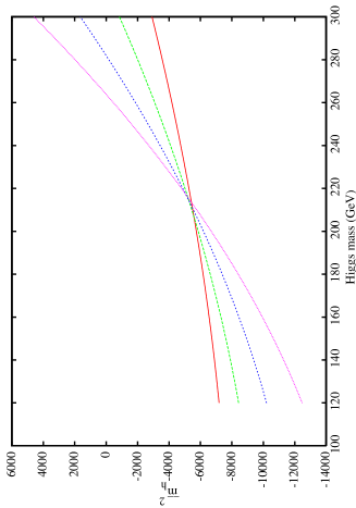
Figure 7: The lower bound on ${\bar{m}_{h}}^{2}$ as a function of the SM Higgs boson mass and $1/R$. $\Lambda R$ is fixed at 20. From top to bottom (at the right-hand edge) are the curves for $1/R=$ 600, 500, 400, and 300 GeV respectively.

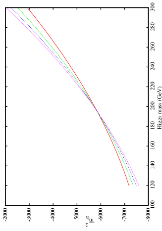
Figure 8: The lower bound on ${\bar{m}_{h}}^{2}$ as a function of the SM Higgs boson mass and $\Lambda R$, $1/R$ being fixed at 300 GeV. From top to bottom (at the right-hand edge) are the curves for $\Lambda R=$ 50, 40, 30, and 20 respectively.

In fig. 7 we show the minimum allowed value of ${\bar{m}_{h}}^{2}$ as a function of $1/R$ and $m_{h}$. These curves are not overly sensitive to the precise value of $\Lambda R$; the dependence is shown in fig. 8. Since ${\bar{m}_{h}}^{2}$ cannot have a large negative value, for most of the parameter space the $\tau$ window will remain open. However, it can have large positive values. For such values, the excited Higgs masses may go above the corresponding electroweak gauge boson masses. This will open up a new set of decay channels, like $H^{0}\to W_{1}^{+}\ell\bar{\nu}_{\ell}$. They are comparable to the two-body channels, since the coupling is a gauge one, not Yukawa. The final state may not have any $\tau$-lepton in them. Since $W_{1}$ lies below the excited quarks, the final state must be hadronically quiet. Also note that for large values of $1/R$ and a heavy SM Higgs boson, the lower limit on ${\bar{m}_{h}}^{2}$ may turn out to be positive. However, this region is mostly outside the reach of ILC.

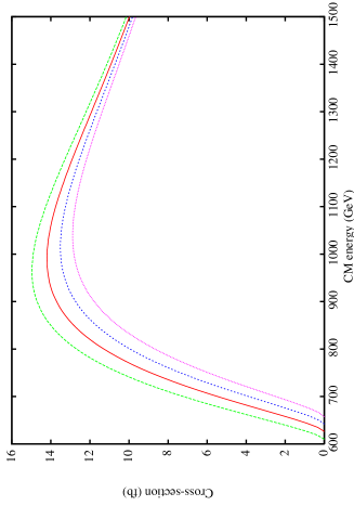
Figure 9: The variation of cross-section for the process $e^{+}e^{-}\to H^{+}H^{-}$ with ${\bar{m}_{h}}^{2}$. From top to bottom, the curves are for ${\bar{m}_{h}}^{2}=-5000$, 0, 5000 and 10000 GeV² respectively. We have fixed $1/R=300$ GeV, $\Lambda R=20$, and the SM Higgs boson mass $m_{h}=120$ GeV.

Is it possible to measure ${\bar{m}_{h}}^{2}$ from precision studies at ILC? For that matter, let us look at the most promising channel, pair production of $H^{+}H^{-}$. In fig. 9 we show how the cross-section changes for different values of ${\bar{m}_{h}}^{2}$. The change is perceptible but may be too small for an experimental detection (also note that the curves are drawn for a favourable point in the parameter space, we may not be so lucky). The problem is further aggravated by the fact that most of the energy in the final state is missing, so it is almost impossible to reconstruct the $H^{+}$ invariant mass. Since leptons, quarks, and gauge bosons do not feel the effect of ${\bar{m}_{h}}^{2}$, we conclude that this is one parameter likely to remain unknown.

V Conclusion

In this paper we have focussed on the possible production, decay, and detection for the $n=1$ excited scalar sector of the Universal Extra Dimension model. These scalars will, with almost 100% branching ratio, decay to soft $n=0$ $\tau$ leptons, accompanied by huge missing energy. Once a UED-type new physics is established at the LHC and subsequently at the ILC (by the study of KK leptons, quarks, and gauge bosons), it seems imperative to study the scalar sector, at least to determine the third and last input parameter to this model, namely, ${\bar{m}_{h}}^{2}$, the boundary mass squared term for the Higgs boson.

Unfortunately, such a thing is easier said than done. By itself, the soft $\tau$ detection is a challenge, but most likely it will be overcome at both LHC and ILC. The problem is to reduce the backgrounds. The SM backgrounds can be removed by judiciously choosing the cuts, but the backgrounds coming from other UED processes (pair production of $W_{1}$, $\tau_{1}$, $\tau_{2}$, $Z_{1}\gamma_{1}$, etc.) are more difficult to handle. For most of the parameter space, such processes give identical signals as the excited scalar production, and with almost identical energies and angular distribution. Thus, it needs a precision study to detect those scalars, and can be performed only at ILC, or CLIC. One may use the excited muon channel as a calibration. The best channel to look for is the charged scalar pair production, for which the signal may just be detected.

Thus, ${\bar{m}_{h}}^{2}$ seems to be one of the most challenging parameter to extract. One can, of course, get a theoretical lower bound on ${\bar{m}_{h}}^{2}$, stemming from the fact that among all the scalars, $H^{+}$ is the lowest-lying, and for sufficiently large negative values of ${\bar{m}_{h}}^{2}$, it can go down below $m_{\gamma_{1}}$ and become the LKP. This sets a lower bound on this term, which is large and negative for most of the parameter space that can be probed at ILC. However, this bound can even be positive for large values of $1/R$ and a large SM Higgs mass. One can say more about this bound once the SM Higgs boson is detected at the LHC.

Acknowledgements

A.K. thanks the Department of Science and Technology, Govt. of India, for the research project SR/S2/HEP-15/2003. He also thanks the Theoretical Physics division of Universität Dortmund, where a part of the work was done, for hospitality. B.B. thanks UGC, Govt. of India, for a research fellowship.

References

-
[1]
G. Nordström, Physik. Zeitschr. 15, 504 (1914);
T. Kaluza, Sitzungsber. D. Preuss. Akademie D. Wissenschaften, Physik.-Mathemat. Klasse, 966 (1921);
O. Klein, Z. Phys. 37, 895 (1926). - [2] E. Cremmer, B. Julia, and J. Scherk, Phys. Lett. B76, 409 (1978).
- [3] T. Appelquist, H.C. Cheng, and B.A. Dobrescu, Phys. Rev. D 64, 035002 (2001).
- [4] G. Servant and T.M.P. Tait, Nucl. Phys. B650, 391 (2003).
- [5] D. Majumdar, Phys. Rev. D 67, 095010 (2003).
- [6] M. Byrne, Phys. Lett. B583, 309 (2004).
- [7] M. Kakizaki, S. Matsumoto, Y. Sato, and M. Senami, Phys. Rev. D 71, 123522 (2005).
-
[8]
K. Kong and K.T. Matchev, J. High Energy Physics 0601, 038 (2006);
T. Flacke, D. Hooper, and J. March-Russell, hep-ph/0509352. - [9] H. Georgi, A.K. Grant and G. Hailu, Phys. Lett. B506, 207 (2001).
- [10] H.C. Cheng, K.T. Matchev, and M. Schmaltz, Phys. Rev. D 66, 036005 (2002).
- [11] M. Puchwein and Z. Kunszt, Annals Phys. 311, 288 (2004).
- [12] See, e.g., I. Antoniadis, Phys. Lett. B246, 377 (1990).
- [13] K. Agashe, N.G. Deshpande, and G.H. Wu, Phys. Lett. B514, 309 (2001).
- [14] D. Chakraverty, K. Huitu, and A. Kundu, Phys. Lett. B558, 173 (2003).
-
[15]
A.J. Buras, M. Spranger, and A. Weiler, Nucl. Phys. B660, 225 (2003);
A.J. Buras, A. Poschenrieder, M. Spranger, and A. Weiler, Nucl. Phys. B678, 455 (2004). - [16] J.F. Oliver, J. Papavassiliou, and A. Santamaria, Phys. Rev. D 67, 056002 (2003).
- [17] J.F. Oliver, hep-ph/0403095.
-
[18]
T.G. Rizzo and J.D. Wells, Phys. Rev. D 61, 016007 (2000);
A. Strumia, Phys. Lett. B466, 107 (1999);
C.D. Carone, Phys. Rev. D 61, 015008 (2000). -
[19]
G. Devidze, A. Liparteliani, and U.-G. Meißner,
Phys. Lett. B634, 59 (2006);
T. Flacke and D.W. Maybury, hep-ph/0601161;
P. Colangelo, F. De Fazio, R. Ferrandes, and T.N. Pham, hep-ph/0604029. - [20] T. Rizzo, Phys. Rev. D 64, 095010 (2001).
- [21] C. Macesanu, C.D. McMullen, and S. Nandi, Phys. Rev. D 66, 015009 (2002).
-
[22]
C. Macesanu, C.D. McMullen, and S. Nandi, Phys. Lett. B546, 253 (2002);
H.C. Cheng, Int. J. Mod. Phys. A18, 2779 (2003);
A. Muck, A. Pilaftsis, and R. Rückl, Nucl. Phys. B687, 55 (2004);
C. Macesanu, S. Nandi, and C.M. Rujoiu, Phys. Rev. D 73, 076001 (2006). - [23] G. Bhattacharyya, P. Dey, A. Kundu, and A. Raychaudhuri, Phys. Lett. B628, 141 (2005).
- [24] M. Battaglia, A. Datta, A. De Roeck, K. Kong and K.T. Matchev, J. High Energy Physics 0507, 033 (2005).
- [25] H.C. Cheng, K.T. Matchev and M. Schmaltz, Phys. Rev. D 66, 056006 (2002).
- [26] S. Riemann, hep-ph/0508136.
- [27] B. Bhattacherjee and A. Kundu, Phys. Lett. B627, 137 (2005).
- [28] S.K. Rai, hep-ph/0510339.
- [29] A.J. Barr, Phys. Lett. B596, 205 (2004).
- [30] J.M. Smillie and B.R. Webber, J. High Energy Physics 0510, 069 (2005).
- [31] A. Datta, K. Kong, and K.T. Matchev, Phys. Rev. D 72, 096006 (2005) [Erratum-ibid. D 72, 119901 (2005)].
- [32] Physics at the CLIC multi-TeV linear collider, hep-ph/0412251, ed. M. Battaglia, A. De Roeck, J. Ellis, D. Schulte.
- [33] A. Pukhov, hep-ph/0412191, and http://www.ifh.de/p̃ukhov/calchep.html.
- [34] See the website: http://hep-www.colorado.edu/SUSY, in particular, N. Danielson, COLO HEP 423. See also, M. Battaglia and D. Schulte, arXiv:hep-ex/0011085; H. Baer, T. Krupovnickas and X. Tata, JHEP 0406 (2004) 061 [arXiv:hep-ph/0405058].