Uncertainty in the leading order PQCD calculations of $B$ meson decays

Abstract

Uncertainty in the PQCD calculation of $B$ decays is investigated in $B\rightarrow\pi$, $B\rightarrow D$ transition form factors and $B\rightarrow D\pi$ decay amplitudes. $B$ meson distribution amplitude dependence is studied by taking three kinds of distribution amplitudes so far suggested. It is found that almost same $q^{2}$ dependence of the form factors can be obtained irrespective of the types of the $B$ meson distribution amplitudes by suitably choosing one parameter. $B\rightarrow D\pi$ process shows the difference due to the distribution amplitude. The effect of the sub-leading component of the $B$ meson distribution amplitude is also studied in the three processes. The numerical results of calculations with the sub-leading component can be well approximated by the leading order calculation with a suitable choice of the distribution amplitude parameters.

I Introduction

$B$ meson decays has been attracting much attention to check the consistency of the standard model (SM) and to explore the existence of a new physics beyond the SM. Two $B$ physics dedicated experimental facilities are constructed at KEK and SLAC. The Belle and the BABAR groups have reported a lot of interesting results since their beginningsBFACS . Many fruitful theoretical works on $B$ physics have been made in these decades, but hadronic effects often obscure the theoretical predictions. Li and collaborators developed the so-called PQCD method and applied it to exclusive $B$ meson decays as one of the approaches to tackle this issueLiPQCD . The PQCD method gives reasonable predictions on $B\rightarrow K\pi$KLS , $B\rightarrow\pi\pi$LUY and other $B$ decaysPQCDB .

In PQCD method, a decay amplitude is obtained as a convolution of a hard part ($H$) and meson distribution amplitudes ($\phi_{k}$).

$$Amp=\int\phi_{1}\times H\times\phi_{2}\cdots\;.$$ (1)

The hard part can in principle be perturbatively calculated in a systematic way, while the non-perturbative contributions are incorporated into the distribution amplitudes. Major uncertainty in the PQCD calculation lies in the choice of distribution amplitudes. We need a model or a non-perturbative method like QCD based sum-rulePB2 ; PB1 ; PB4 ; BB to obtain the distribution amplitudes. Meson distribution amplitudes are important also in the study of $B$ non-leptonic decays with QCD factorization methodBBNS and in the calculation of the form factors with QCD based sum-rule schemePB1 ; PB4 . So far most of the PQCD calculations of $B$ decays are given in the leading order of $\alpha_{S}$ and $1/M$. (A trial to estimate the higher order effects in $\alpha_{S}$ is given in MSSA .) The aim of this paper is to investigate the uncertainty of the leading order PQCD calculations. Our strategy is as follows: In Sec.II, we analyze $B\rightarrow\pi$ form factors to estimate the uncertainty due to the factors given below;

1. $B$ meson distribution amplitude: $B\rightarrow\pi$ form factors are calculated by adopting three kinds of $B$ meson distribution amplitudes proposed in the previous worksGN ; KLS ; KKQT . The parameters of $B$ meson distribution amplitudes are fixed to accommodate with the reasonable value of the form factor at $q^{2}=0$. Then we vary these parameters to see how the value of the form factor changes.

2. Pion distribution amplitude: We adopt the distribution amplitude given in QCD based sum-rule analysisPB2 ; PB1 , and investigate the dependence on the parameters of those distribution amplitudes. (The effect of choosing another pion distribution amplitude is investigated in HuWu .)

3. Hard part: The dependence on $\Lambda_{QCD}$ and other renormalization group parameters are investigated.

4. Sub-leading contributions: We estimate the $O(1/M)$ corrections in the hard part and the contributions from the sub-leading component of the $B$ meson distribution amplitude.

In Sec. III, we analyze $B\rightarrow D$ form factors. The parameters of $B$ meson distribution amplitudes are fixed by the first analysis. Here, we investigate the dependence on the parameter of the $D$ meson distribution amplitude proposed in TLS2 . In Sec. IV, we analyze $B\rightarrow D\pi$ decays by using the $B$, $D$ and pion distribution amplitudes fixed in the previous analyses. The non-factorizable contribution is important in $B\rightarrow D\pi$ decays KKLL . We show which $B$ meson distribution amplitude gives better results by calculating the non-factorizable contribution. Sec. V is devoted to summary and discussions.

II Heavy-to-light Form Factors

We first analyze the $B\rightarrow\pi$ form factors in the fast recoil region with PQCD method. We shall determine the parameters of $B$ meson distribution amplitudes from the $B\to\pi$ form factors. The $B\to\pi$ transition form factors $F^{B\pi}_{+}$ and $F^{B\pi}_{0}$ are defined by the matrix element,

$$\langle\pi(P_{2})|{\bar{b}}(0)\gamma_{\mu}u(0)|B(P_{1})\rangle=F^{B\pi}_{+}(q^{2})\left[(P_{1}+P_{2})_{\mu}-\frac{m_{B}^{2}-m_{\pi}^{2}}{q^{2}}q_{\mu}\right]+F^{B\pi}_{0}(q^{2})\frac{m_{B}^{2}-m_{\pi}^{2}}{q^{2}}q_{\mu}\;,$$ (2)

where $q=P_{1}-P_{2}$ is the lepton-pair momentum. Another equivalent definition is

$$\langle\pi(P_{2})|{\bar{b}}(0)\gamma_{\mu}u(0)|B(P_{1})\rangle=f_{1}(q^{2})P_{1\mu}+f_{2}(q^{2})P_{2\mu}\;,$$ (3)

in which the form factors $f_{1}$ and $f_{2}$ are related to $F^{B\pi}_{+}$ and $F^{B\pi}_{0}$ by

$$F^{B\pi}_{+} = \frac{1}{2}(f_{1}+f_{2})\;,$$ (4)

$$F^{B\pi}_{0} = \frac{1}{2}f_{1}\left(1+\frac{q^{2}}{m_{B}^{2}}\right)+\frac{1}{2}f_{2}\left(1-\frac{q^{2}}{m_{B}^{2}}\right)\;.$$ (5)

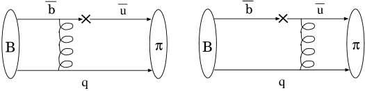
In PQCD method, the form factors $F^{B\pi}_{+,0}$ are derived from the diagrams with one hard gluon exchange shown in Fig. 1. PQCD works best in the region with large energy transfer, i.e., with small $q^{2}$. Soft contribution from the diagram without any hard gluon is Sudakov suppressedTLS .

Figure 1: Leading-order contribution to $F^{B\pi}$.

The formulae for the $B\to\pi$ form factors are given as

$$f_{1} = 16\pi m_{B}^{2}C_{F}r_{\pi}\int dx_{1}dx_{2}\int b_{1}db_{1}b_{2}db_{2}\phi_{B}(x_{1},b_{1})[\phi_{\pi}^{p}(x_{2})-\phi_{\pi}^{t}(x_{2})]$$ (6)

$$\times E(t^{(1)})h(x_{1},x_{2},b_{1},b_{2})\;,$$

$$f_{2} = 16\pi m_{B}^{2}C_{F}\int dx_{1}dx_{2}\int b_{1}db_{1}b_{2}db_{2}\phi_{B}(x_{1},b_{1})$$ (7)

$$\times \Biggl{\{}\left[\phi_{\pi}(x_{2})(1+x_{2}\eta)+2r_{\pi}\left((\frac{1}{\eta}-x_{2})\phi_{\pi}^{t}(x_{2})-x_{2}\phi_{\pi}^{p}(x_{2})\right)\right]E(t^{(1)})h(x_{1},x_{2},b_{1},b_{2})$$

$$+2r_{\pi}\phi_{\pi}^{p}E(t^{(2})h(x_{2},x_{1},b_{2},b_{1})\Biggr{\}}\;,$$

with $\eta=2P_{1}\cdot P_{2}/m_{B}^{2}=1-(q^{2}/m_{B}^{2})$, the ratio $r_{\pi}=m_{0}/m_{B}$ ($m_{0}$: chiral mass of pion) and the evolution factor

$$E(t)=\alpha_{s}(t)e^{-S_{B}(t)-S_{\pi}(t)}\;,$$ (8)

where $S_{B}$ and $S_{\pi}$ are the Sudakov factor of $k_{T}$ part for $B$ meson and pion, respectivelyTLS . The hard function is given as

$$h(x_{1},x_{2},b_{1},b_{2}) = S_{t}(x_{2})K_{0}\left(\sqrt{x_{1}x_{2}\eta}m_{B}b_{1}\right)$$ (9)

$$\times\left[\theta(b_{1}-b_{2})K_{0}\left(\sqrt{x_{2}\eta}m_{B}b_{1}\right)I_{0}\left(\sqrt{x_{2}\eta}m_{B}b_{2}\right)\right.$$

$$\left.+\theta(b_{2}-b_{1})K_{0}\left(\sqrt{x_{2}\eta}m_{B}b_{2}\right)I_{0}\left(\sqrt{x_{2}\eta}m_{B}b_{1}\right)\right]\;,$$

where the factor $S_{t}$ is the threshold resummation factor

$$S_{t}(x)=\frac{2^{1+2c}\Gamma(3/2+c)}{\sqrt{\pi}\Gamma(1+c)}[x(1-x)]^{c}\;,$$ (10)

which suppresses the end-point behaviors of the meson distribution amplitudes. The hard scales $t^{(1),(2)}$ are defined as

$$t^{(1)} = {\rm max}(\sqrt{x_{2}\eta}m_{B},1/b_{1},1/b_{2})\;,$$

$$t^{(2)} = {\rm max}(\sqrt{x_{1}\eta}m_{B},1/b_{1},1/b_{2})\;.$$ (11)

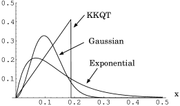
We investigate here the following candidates of $B$ meson distribution amplitude:

$$\phi_{B}^{KLS}(x,b) = N_{B}^{KLS}x^{2}(1-x)^{2}\exp\left[-\frac{1}{2}\left(\frac{xm_{B}}{\omega_{KLS}}\right)^{2}-\frac{\omega_{KLS}^{2}b^{2}}{2}\right]\;,$$ (12)

$$\phi_{B}^{GN}(x,b) = N_{B}^{GN}x\;\exp\left[-\frac{xm_{B}}{\omega_{GN}}\right]\frac{1}{1+(b\omega_{GN})^{2}}\;,$$ (13)

$$\phi_{B}^{KKQT}(x,b) = N_{B}^{KKQT}x\;\theta(x)\theta(\frac{2\Lambda_{KKQT}}{m_{B}}-x)J_{0}\left(b\sqrt{x(\frac{2\Lambda_{KKQT}}{m_{B}}-x)}\right)\;.$$ (14)

The first one, which we call Gaussian type, is proposed in KLS . The $x$ dependence of the second one, which we call exponential type, is proposed in GN , and we take its $b$ dependence as Lorentzian, the Fourier transform of the exponential function. The third one, which we call KKQT type, is obtained by solving the equations of motion under the approximation of neglecting 3-parton contributionsKKQT . Each candidate is parameterized by one parameter, $\omega_{KLS}$, $\omega_{GN}$ or $\Lambda_{KKQT}$. The normalization constant $N_{B}$ is related to the decay constant $f_{B}$ through the relation

$$\int dx\;\phi_{B}(x,0)=\frac{f_{B}}{2\sqrt{2N_{c}}}\;.$$ (15)

The shapes of these $B$ meson distribution amplitude with $b=0$ are shown in Fig. 2, where the parameters are chosen so that $F^{B\pi}_{+,0}(0)\cong 0.3$ as explained later.

Figure 2: $\phi_{B}(x,0)$ for $\omega_{KLS}=0.38$, $\omega_{GN}=0.36$ and $\Lambda_{KKQT}/M_{B}=0.094$,

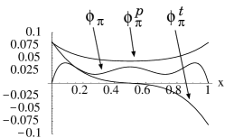
In Eqs. (6) and (7) we have included the two-parton twist-3 distribution amplitudes $\phi^{p}_{\pi}$ and $\phi^{t}_{\pi}$ associated with the pseudo-scalar and pseudo-tensor structures of the pion, respectivelyPB2 . The contribution from the axial vector component $\phi_{\pi}$ is twist-2. The pion distribution amplitudes derived from QCD based sum rule are given asPB1

$$\phi_{\pi}(x) = \frac{3f_{\pi}}{\sqrt{2N_{c}}}x(1-x)\left[1+a_{2}C_{2}^{3/2}(1-2x)+a_{4}C_{4}^{3/2}(1-2x)\right]\;,$$ (16)

$$\phi_{\pi}^{p}(x) = \frac{f_{\pi}}{2\sqrt{2N_{c}}}\left[1+a_{2p}C_{2}^{1/2}(1-2x)+a_{4p}C_{4}^{1/2}(1-2x)\right]\;,$$ (17)

$$\phi_{\pi}^{t}(x) = \frac{f_{\pi}}{2\sqrt{2N_{c}}}(1-2x)\left[1+6a_{2t}(10x^{2}-10x+1)\right]\;.$$ (18)

The coefficients $a_{2}\;,\dots,a_{2t}$ are defined asPB5

$$a_{2}(1\text{ GeV}) = 0.44\ ,\ a_{4}(1\text{ GeV})=0.25$$ (19)

$$a_{2p} = 30\eta_{3}-\frac{5}{2}\rho_{\pi}^{2}\ ,\ a_{4p}=-(3\eta_{3}\omega_{3}+\frac{27}{20}\rho_{\pi}^{2}+\frac{81}{10}\rho_{\pi}^{2}a_{2}),$$ (20)

$$a_{2t} = 5\eta_{3}-\frac{1}{2}\eta_{3}\omega_{3}-\frac{7}{20}\rho_{\pi}^{2}-\frac{3}{5}\rho_{\pi}^{2}a_{2},$$ (21)

where

$$\rho_{\pi}^{2} = \frac{(m_{d}+m_{u})}{m_{0}}=\frac{m_{\pi}^{2}}{m_{0}^{2}}\ ,$$ (22)

$$a_{k}(\mu) = \left[\frac{\alpha_{s}(\mu)}{\alpha_{s}(\mu_{0})}\right]^{\gamma_{k}/b}a_{k}(\mu_{0})\ ,\ b=11-\frac{2}{3}N_{F}\ ,$$ (23)

$$\gamma_{k} = 4C_{F}\left[\psi(k+2)+\gamma_{E}-\frac{3}{4}-\frac{1}{2(k+1)(k+2)}\right]\ ,$$ (24)

$$\eta_{3}(\mu) = \left[\frac{\alpha_{s}(\mu)}{\alpha_{s}(\mu_{0})}\right]^{\gamma^{\eta}_{3}/b}\eta_{3}(\mu_{0})\ ,\ \gamma^{\eta}_{3}=\frac{16}{3}C_{F}+N_{C},$$ (25)

$$\omega_{3}(\mu) = \left[\frac{\alpha_{s}(\mu)}{\alpha_{s}(\mu_{0})}\right]^{\gamma^{\omega}_{3}/b}\omega_{3}(\mu_{0})\ ,\ \gamma^{\omega}_{3}=-\frac{25}{6}C_{F}+\frac{7}{3}N_{C}\ ,$$ (26)

with $\eta_{3}(1\text{ GeV})=0.015$, $\omega_{3}(1\text{ GeV})=-3$. The Gegenbauer polynomials are defined by

$$C_{2}^{1/2}(t)=\frac{1}{2}(3t^{2}-1)\;,\;\;\;C_{4}^{1/2}(t)=\frac{1}{8}(35t^{4}-30t^{2}+3)\;,$$

$$C_{2}^{3/2}(t)=\frac{3}{2}(5t^{2}-1)\;,\;\;\;C_{4}^{3/2}(t)=\frac{15}{8}(21t^{4}-14t^{2}+1)\;.$$ (27)

Figure 3: $\phi_{\pi}(x)$, $\phi^{p}_{\pi}(x)$ and $\phi^{t}_{\pi}(x)$ for default values of inputs.

II.1 Numerical results

We present the numerical results of the $B\rightarrow\pi$ transition form factors given above. The default values for inputs are given as follows:

$$\begin{array}[]{ccc}f_{B}=190\text{ MeV}\ ,&f_{\pi}=130\text{ MeV}\ ,&\Lambda_{\rm QCD}=250\text{ MeV ($N_{f}=4$)}\ ,\\ c=0.3\ ,&m_{0}=1.4\text{ GeV}\ ,&\\ a_{2}=0.44\ ,&a_{4}=0.25\ ,&a_{2p}=0.43\ ,\\ a_{4p}=0.09\ ,&a_{2t}=0.55/6\ .&\end{array}$$ (28)

The parameters in $B$ meson distribution amplitudes are chosen as $\omega_{KLS}=0.38$, $\omega_{GN}=0.36$ and $\Lambda_{KKQT}/M_{B}=0.094$ so that we have $F^{B\pi}_{+,0}(0)\cong 0.3$, which is reasonable in comparison with the sum-rule resultsPB4 . We neglect the scale dependence of parameters $m_{0}$ and $a_{2}\;,\dots,a_{2t}$ in the default calculation. Its effect shall be discussed later. Monte-Carlo method is used to evaluate the numerical integrals. We have set the number of samples so that the statistical errors in Monte-Carlo integrations may be less than 0.1%. The values of two form factors should be equal at $q^{2}=0$. The PQCD results becomes unreliable gradually at slow recoil. Our results of $F^{B\pi}_{+}(q^{2})$ and $F^{B\pi}_{0}(q^{2})$ for $q^{2}=0\sim 10$ GeV² are shown in Table 1 and Fig. 4. It can be seen that the $q^{2}$ dependences are almost same irrespective of the choice of the $B$ meson distribution amplitude. The difference is at most 4 % at $q^{2}=10$ GeV². The ratio of each contribution from $\phi_{\pi}$, $\phi^{p}_{\pi}$ and $\phi^{t}_{\pi}$ to the total value of $F^{B\pi}_{+}(0)$ is given in Table 2. It shows that the twist-3 contribution is important as explained in TLS .

Gaussian type with $\omega_{KLS}=0.38$:
$q^{2}$ (GeV²) 0.0 1.0 2.0 3.0 4.0 5.0 6.0 7.0 8.0 9.0 10.0 $F^{B\pi}_{0}$ 0.297 0.310 0.324 0.339 0.355 0.374 0.393 0.416 0.441 0.468 0.499 $F^{B\pi}_{+}$ 0.297 0.321 0.347 0.377 0.411 0.450 0.494 0.546 0.605 0.674 0.756

Exponential type with $\omega_{GN}=0.36$:
$q^{2}$ (GeV²) 0.0 1.0 2.0 3.0 4.0 5.0 6.0 7.0 8.0 9.0 10.0 $F^{B\pi}_{0}$ 0.300 0.312 0.325 0.339 0.356 0.373 0.391 0.413 0.436 0.461 0.490 $F^{B\pi}_{+}$ 0.300 0.323 0.349 0.378 0.412 0.449 0.492 0.542 0.599 0.665 0.743

KKQT type with $\displaystyle\frac{\Lambda_{KKQT}}{m_{B}}=0.094$:
$q^{2}$ (GeV²) 0.0 1.0 2.0 3.0 4.0 5.0 6.0 7.0 8.0 9.0 10.0 $F^{B\pi}_{0}$ 0.299 0.313 0.327 0.342 0.359 0.378 0.399 0.422 0.447 0.476 0.508 $F^{B\pi}_{+}$ 0.299 0.324 0.351 0.381 0.415 0.456 0.501 0.554 0.615 0.686 0.770

Table 1: Numerical outputs of $F^{B\pi}_{0}(q^{2})$ and $F^{B\pi}_{+}(q^{2})$

	Gaussian	Exponential	KKQT
$\phi_{\pi}$ (%)	40	37	40
$\phi^{p}_{\pi}$ (%)	47	51	46
$\phi^{t}_{\pi}$ (%)	13	12	14

Table 2: The contributions from $\phi_{\pi}$, $\phi^{p}_{\pi}$ and $\phi^{t}_{\pi}$ to the total value of $F^{B\pi}(0)$.

Figure 4: The $B\to\pi$ form factors $F^{B\pi}_{+}$ and $F^{B\pi}_{0}$ as functions of $q^{2}$ (GeV²). The results by Gaussian, exponential and KKQT type B distribution amplitude are shown in solid, dot and dot-dashed line, respectively.

II.2 Parameters in distribution amplitudes

Each of the $B$ meson distribution amplitudes, Eqs. (12), (13) and (14), adopted in the previous calculation has only one parameter $\omega_{KLS}$, $\omega_{GN}$ and $\Lambda_{KKQT}$, respectively. The pion distribution amplitudes, Eqs. (16)-(18), contain 5 parameters, $m_{0}^{\pi}$, $a_{1}$, $a_{2}$, $\eta_{3}$ and $\omega_{3}$. We study how the numerical outputs of the form factors at $q^{2}=0$ vary with these parameters. The form factor at $q^{2}=0$ can be rewritten by factoring out the parameters in the pion distribution amplitudes as

$$F^{B\pi}(0) = F^{A0}(X)+a_{2}F^{A2}(X)+a_{4}F^{A4}(X)+\frac{m_{0}}{m_{B}}\left[F^{P0}(X)+a_{2p}F^{P2}(X)\right.$$ (30)

$$\left.+a_{4p}F^{P4}(X)+F^{T0}(X)+a_{2t}F^{T2}(X)\right],$$

where $X=\omega_{KLS}$, $\omega_{GN}$ or $\Lambda_{KKQT}$. The functions $F^{A0}$, $F^{A2}$ … $F^{T2}$ do not depend on the pion parameters.

Gaussian type:

In the case of Gaussian type $B$ meson distribution amplitude, the $\omega_{KLS}$ dependence can be well approximated within 1% precision for $0.28\leq\omega_{KLS}\leq 0.48$ by the following formulae;

$$F^{A0}(\omega_{KLS}) = 0.0623-0.175\,(\omega_{KLS}-0.38)+0.382\,(\omega_{KLS}-0.38)^{2}-0.784\,(\omega_{KLS}-0.38)^{3}\;,$$

$$F^{A2}(\omega_{KLS}) = 0.0860-0.246\,(\omega_{KLS}-0.38)+0.455\,(\omega_{KLS}-0.38)^{2}-0.634\,(\omega_{KLS}-0.38)^{3}\;,$$

$$F^{A4}(\omega_{KLS}) = 0.0784-0.231\,(\omega_{KLS}-0.38)+0.417\,(\omega_{KLS}-0.38)^{2}-0.242\,(\omega_{KLS}-0.38)^{3}\;,$$

$$F^{P0}(\omega_{KLS}) = 0.446-1.98\,(\omega_{KLS}-0.38)+6.47\,(\omega_{KLS}-0.38)^{2}-17.5\,(\omega_{KLS}-0.38)^{3}\;,$$

$$F^{P2}(\omega_{KLS}) = 0.153-0.563\,(\omega_{KLS}-0.38)+1.34,(\omega_{KLS}-0.38)^{2}-2.05\,(\omega_{KLS}-0.38)^{3}\;,$$

$$F^{P4}(\omega_{KLS}) = 0.0825-0.288\,(\omega_{KLS}-0.38)+0.591\,(\omega_{KLS}-0.38)^{2}-0.471\,(\omega_{KLS}-0.38)^{3}\;,$$

$$F^{T0}(\omega_{KLS}) = 0.109-0.332\,(\omega_{KLS}-0.38)+0.635\,(\omega_{KLS}-0.38)^{2}-0.734\,(\omega_{KLS}-0.38)^{3}\;,$$

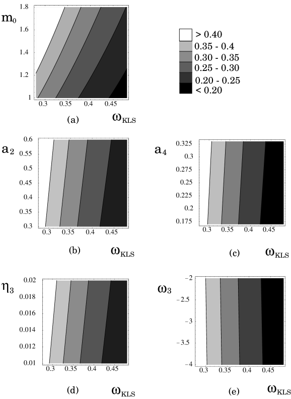
$$F^{T2}(\omega_{KLS}) = 0.441-1.37\,(\omega_{KLS}-0.38)+2.64\,(\omega_{KLS}-0.38)^{2}-3.86\,(\omega_{KLS}-0.38)^{3}\;.$$ (31)

The chiral mass $m_{0}=m_{\pi}^{2}/(m_{u}+m_{d})$ plays an important role in hadron dynamics. It gives penguin enhancement in $B$ meson non-leptonic decays as pointed out in KLS . It is essential for the form factor calculation to take into account of the important higher-twist contributionsTLS . The chiral mass $m_{0}$ enters in Eqs. (6) and (7) as $r_{\pi}=m_{0}/m_{B}$ and in the parameter $\rho_{\pi}$ of Gegenbauer polynomials in the pion distribution amplitudes. (See Eqs. (20)-(22).) The $r_{\pi}$ dependence of the from factor is linear, while the parameter $\rho_{\pi}$ in pion distribution amplitudes depends linearly on $1/m_{0}$. The $m_{0}$ dependence of $a_{2p}$, $a_{4p}$ and $a_{2t}$ through $\rho^{2}$ can be neglected since $\rho_{\pi}^{2}=O(10^{-2})$. The $\omega_{KLS}$ - $m_{0}$ dependence of $F^{B\pi}(0)$ is shown in Fig. 5 (a), where other parameters are fixed to the default values. The dependence on other inputs are also shown in Figs. 5 (b)-(e).

Exponential type:

The similar calculation is done in the case of the exponential type $B$ meson distribution amplitude. The $\omega_{GN}$ dependence is obtained for $0.26\leq\omega_{GN}\leq 0.46$. The approximation formulae of $F^{A0}\sim F^{T2}$ are given in the appendix A. The result is shown in Fig. 6.

KKQT type:

The result in the case of the KKQT type $B$ meson distribution amplitude is shown in Fig. 7. The $\Lambda_{KKQT}$ dependence is obtained for $0.074\leq\Lambda_{KKQT}/M_{B}\leq 0.114$. The approximation formulae of $F^{A0}\sim F^{T2}$ are given in the appendix A.

Figure 5: Contour plots of $F^{B\pi}(0)$. (a) $\omega_{KLS}$ - $m_{0}$, (b) $\omega_{KLS}$ - $a_{2}$ (c) $\omega_{KLS}$ - $a_{4}$, (d) $\omega_{KLS}$ - $\eta_{3}$ (e) $\omega_{KLS}$ - $\omega_{3}$. The values of $F^{B\pi}(0)$ are shown by using shades as given in the sample .

Figure 6: Contour plots of $F^{B\pi}(0)$. (a) $\omega_{GN}$ - $m_{0}$, (b) $\omega_{GN}$ - $a_{2}$ (c) $\omega_{GN}$ - $a_{4}$, (d) $\omega_{GN}$ - $\eta_{3}$ (e) $\omega_{GN}$ - $\omega_{3}$. The values of $F^{B\pi}(0)$ are shown by using shades as given in the sample .

Figure 7: Contour plots of $F^{B\pi}(0)$. (a) $\Lambda_{KKQT}$ - $m_{0}$, (b) $\Lambda_{KKQT}$ - $a_{2}$ (c) $\Lambda_{KKQT}$ - $a_{4}$, (d) $\Lambda_{KKQT}$ - $\eta_{3}$ (e) $\Lambda_{KKQT}$ - $\omega_{3}$. $\Lambda_{KKQT}$ is given in unit of $M_{B}$. The values of $F^{B\pi}(0)$ are shown by using shades as given in the sample .

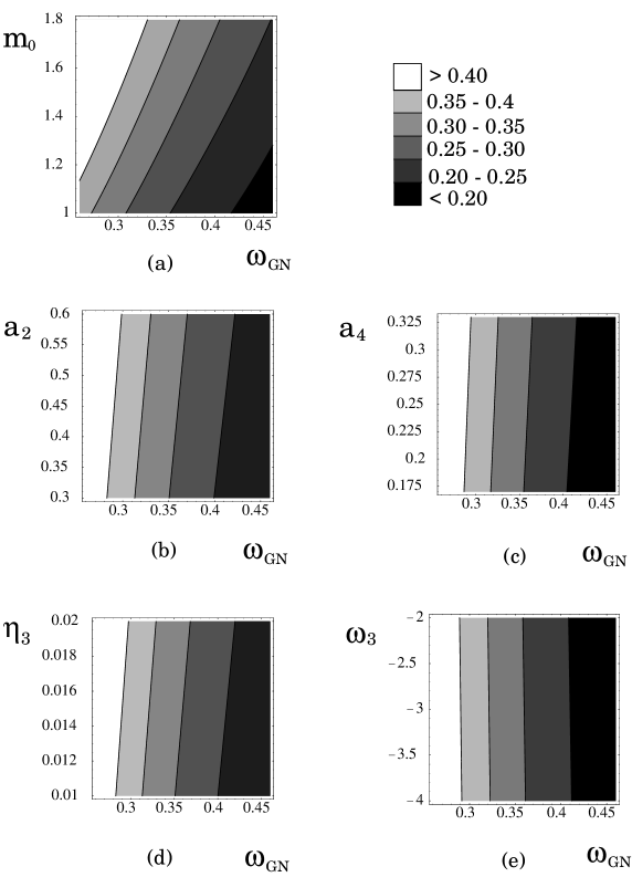
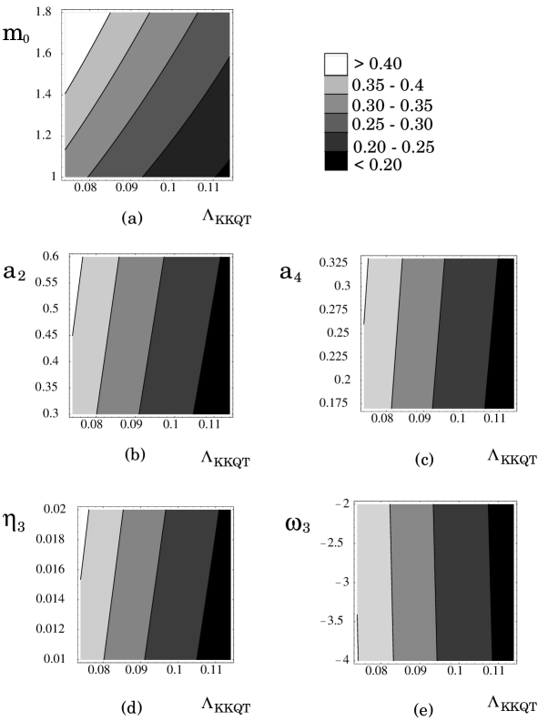
These figures show that $F^{B\pi}(0)$ depends most significantly on $m_{0}$ and a $B$ meson distribution amplitude parameter ($\omega_{B}$, $\omega_{GN}$ or $\Lambda_{KKQT}$). The change of other parameters within reasonable range affects on $F^{B\pi}(0)$ at most 10%.

The $B$ meson decay constant, $f_{B}$, is concerned solely with the normalization of $B$ meson wave function in the form factor calculation. The normalization constant $N_{B}$ enters linearly in our calculation. So if $f_{B}$ changes to $f_{B}+\Delta f_{B}$, the output changes to $(1+\Delta f_{B}/f_{B})$ times the original value. This is also the case in the calculation of non-leptonic decays

II.3 Intrinsic $b$ dependence

We investigate the uncertainty from the intrinsic $b$ dependence of light meson distribution amplitudes, which are advocated by Kroll et al.bdepK . The $b$ dependence of pion is taken to be the following form bdepK ,

$$\exp\left[-\frac{x(1-x)b^{2}}{4a_{\pi}^{2}}\right]\;,$$ (32)

where $a_{\pi}$ is the transverse size parameter of the pion. We take $a_{\pi}^{-1}\simeq\sqrt{8}\pi f_{\pi}$ here. The variation of $F^{B\pi}(0)$ under the influence of the above $b$ dependence of pion distribution amplitude is shown in Table 3. The effects of intrinsic $b$ dependence is estimated to be about 10% or less.

$a_{\pi}^{-1}$	Gaussian	Exponential	KKQT
without $b$ dependence	0.297	0.300	0.299
$0.8\times\sqrt{8}\pi f_{\pi}$	0.284	0.285	0.286
$\sqrt{8}\pi f_{\pi}$	0.277	0.278	0.279
$1.2\times\sqrt{8}\pi f_{\pi}$	0.269	0.269	0.272

Table 3: $b$ dependence of $F^{B\pi}(0)$

II.4 Evolution effect

II.4.1 Gegenbauer coefficients

The Gegenbauer coefficients in the light meson distribution amplitudes depend on the energy scale. In the PQCD calculation it evolves with the scale $1/b$ governed by $[\alpha_{s}(1/b)/\alpha_{s}(\mu_{0})]^{\gamma/b}$ ($b=11-2N_{f}/3$), where $\mu_{0}$ represents the initial scale the evolution starts with, and $\gamma$ is an anomalous dimension BB . We have investigated this evolution effect. Calculations are made by taking the evolution effect into account. It can be seen from Table 4 that the effect is about 10%, and can be covered by the theoretical uncertainty from the variation of the Gegenbauer coefficients.

$\mu_{0}$ (GeV)	Gaussian	Exponential	KKQT
no evolution	0.297	0.300	0.299
0.5	0.347	0.345	0.352
1.0	0.294	0.297	0.298
1.5	0.278	0.282	0.280

Table 4: The evolution effect on $F^{B\pi}(0)$

II.4.2 $\Lambda_{\rm QCD}$

The QCD coupling constant $\alpha_{S}$ appears explicitly and implicitly through the resummation factor $S$ in Eq. (8). The QCD scale $\Lambda_{\rm QCD}$ determines $\alpha_{S}$. Let us see how the form factor values varies depending on $\Lambda_{\rm QCD}$. The result is given in Table 5, which shows that change in the form factor values is about 3% for $200\text{ MeV}\leq\Lambda_{\rm QCD}\leq 300\text{ MeV}$.

$\Lambda_{\rm QCD}$ (MeV)	Gaussian	Exponential	KKQT
200	0.299	0.308	0.310
225	0.298	0.305	0.306
250	0.297	0.300	0.299
275	0.293	0.294	0.294
300	0.289	0.288	0.286

Table 5: $\Lambda_{\rm QCD}$ dependence of $F^{B\pi}(0)$

II.4.3 Hard scales

The scale of $\alpha_{s}$ in the expression of the form factors is determined in Eq. (11). This choice is not unique, because the next leading order correction has not been calculated. There is another candidate of the scale:

$$t^{(1)}=t^{(2)}={\rm max}(\sqrt{x_{1}\eta}m_{B},\sqrt{x_{2}\eta}m_{B},1/b_{1},1/b_{2})\;,$$ (33)

The change of the value of $F^{B\pi}(0)$ under the choice of hard scale is shown in Table 6. For reference, we also show the value in the case of the fixed hard scales; $t^{(1)}=t^{(2)}=M_{B}/2$, $M_{B}$, $2M_{B}$. The result shows that $F^{B\pi}(0)$ changes about 10% or less depending on the choice of the form of the scale $t^{(1,2)}$.

	Gaussian	Exponential	KKQT
original	0.297	0.300	0.299
Eq. (33)	0.288	0.290	0.289
fixed $t^{(1)}=t^{(2)}=M_{B}/2$	0.286	0.288	0.288
fixed $t^{(1)}=t^{(2)}=M_{B}$	0.276	0.277	0.277
fixed $t^{(1)}=t^{(2)}=2M_{B}$	0.269	0.270	0.270

Table 6: Scale choice dependence of $F^{B\pi}(0)$

II.4.4 Threshold resummation factors

There is a source of theoretical uncertainty from the threshold resummation factor $c$ in Eq. (10). Note that this uncertainty, whose property differs from others like $m_{0}$, is not due to an unknown parameter, but to our parameterization. In principle, we can adopt the exact resummation result, such that no theoretical uncertainty is associated with it.

II.5 Sub-leading contribution

II.5.1 $O(\Lambda_{hadron}/m_{B})$ terms

The formulae of the form factors $f_{1}$ and $f_{2}$ are the leading order results where the terms proportional to $x_{1}\sim\Lambda_{hadron}/m_{B}$ are neglected. If we do not neglect them, the following terms are added.

$$\Delta f_{1} = 16\pi m_{B}^{2}C_{F}\int dx_{1}dx_{2}\int b_{1}db_{1}b_{2}db_{2}\phi_{B}(x_{1},b_{1})x_{1}(\eta\phi_{\pi}-2r_{\pi}\phi^{p}_{\pi})$$ (34)

$$\times E(t^{(2)})h(x_{2},x_{1},b_{2},b_{1})\;,$$

$$\Delta f_{2} = 16\pi m_{B}^{2}C_{F}\int dx_{1}dx_{2}\int b_{1}db_{1}b_{2}db_{2}\phi_{B}(x_{1},b_{1})x_{1}\left(-\phi_{\pi}+\frac{2r_{\pi}}{\eta}\phi^{p}_{\pi}\right)$$ (35)

$$\times E(t^{(2})h(x_{2},x_{1},b_{2},b_{1})\;,$$

The numerical outputs of the above quantities are given in Table 7. It can be fond that the sub-leading contribution from $x_{1}$ terms is about 4% of the leading value.

Gaussian	Exponential	KKQT
0.040	0.035	0.041

Table 7: $\Delta F^{B\pi}(0)/F^{B\pi}(0)$

The leading order results of PQCD calculation are obtained under the approximation of $M_{B}=m_{b}$. If we do not take this approximation the formulae become as follows;

$$f_{1} = 16\pi m_{B}^{2}C_{F}r_{\pi}\int dx_{1}dx_{2}\int b_{1}db_{1}b_{2}db_{2}\phi_{B}(x_{1},b_{1})[(1+r_{B})\phi_{\pi}^{p}(x_{2})-(1-r_{B})\phi_{\pi}^{t}(x_{2})]$$ (36)

$$\times E(t^{(1)})h_{B}(x_{1},x_{2},b_{1},b_{2})\;,$$

$$f_{2} = 16\pi m_{B}^{2}C_{F}\int dx_{1}dx_{2}\int b_{1}db_{1}b_{2}db_{2}\phi_{B}(x_{1},b_{1})$$ (37)

$$\times \Biggl{\{}\left[\phi_{\pi}(x_{2})(1+x_{2}\eta-r_{B})+2r_{\pi}\left((1-\frac{r_{B}}{2})(\frac{1}{\eta}-x_{2})\phi_{\pi}^{t}(x_{2})-x_{2}\phi_{\pi}^{p}(x_{2})\right)\right]E(t^{(1)})h_{B}(x_{1},x_{2},b_{1},b_{2})$$

$$+2r_{\pi}\phi_{\pi}^{p}E(t^{(2})h(x_{2},x_{1},b_{2},b_{1})\Biggr{\}}\;,$$

where $r_{B}=\bar{\Lambda}/M_{B}=(M_{B}-m_{b})/M_{B}$. The hard function $h_{B}$ is given as

$$h_{B}(x_{1},x_{2},b_{1},b_{2}) = S_{t}(x_{2})K_{0}\left(\sqrt{x_{1}x_{2}\eta}m_{B}b_{1}\right)$$ (38)

$$\times\theta(x_{2}\eta-2r_{B})\left[\theta(b_{1}-b_{2})K_{0}\left(\sqrt{x_{2}\eta-2r_{B}}m_{B}b_{1}\right)I_{0}\left(\sqrt{x_{2}\eta-2r_{B}}m_{B}b_{2}\right)\right.$$

$$\left.+\theta(b_{2}-b_{1})K_{0}\left(\sqrt{x_{2}\eta-2r_{B}}m_{B}b_{2}\right)I_{0}\left(\sqrt{x_{2}\eta-2r_{B}}m_{B}b_{1}\right)\right]\;.$$

The outputs of $F^{B\pi}(0)$ with the above formulae are given in Table 8. Comparing this result with the leading order one, we find that the effect of this approximation is about 2%.

Gaussian	Exponential	KKQT
0.302	0.305	0.304

Table 8: $F^{B\pi}(0)$ without taking $M_{B}=m_{b}$

II.5.2 Another component of $B$ distribution amplitudes

The $B$ meson distribution amplitude in fact consists of two componentsGN ;

$$\Phi_{B}=-\frac{i}{\sqrt{2N_{c}}}(\not P+m_{B})\gamma_{5}\left[\not{v_{+}}\phi_{B}^{+}(k)+\not{v_{-}}\phi_{B}^{-}(k)\right]\;,$$ (39)

where $v=P/m_{B}=v_{+}+v_{-}$ with $v_{+}=((v^{0}+v^{3})/\sqrt{2},0,0_{T})$ and $v_{-}=(0,(v^{0}-v^{3})/\sqrt{2},0_{T})$. The spatial direction of the velocity $v$ is taken along the third direction ($v^{1}=v^{2}=0$). By using the identity $(\not P+m_{B})\gamma_{5}(1+\not v)=0$, we can add an arbitrary function $f$ in the above expression;

$$\Phi_{B} \propto (\not P+m_{B})\gamma_{5}\left[\not{v_{+}}\phi_{B}^{+}+\not{v_{-}}\phi_{B}^{-}\right]$$ (40)

$$= (\not P+m_{B})\gamma_{5}\left[\not{v_{+}}\phi_{B}^{+}+\not{v_{-}}\phi_{B}^{-}+(1+\not v)f\right]$$

$$= (\not P+m_{B})\gamma_{5}\left[f+\not{v_{+}}(\phi_{B}^{+}+f)+\not{v_{-}}(\phi_{B}^{-}+f)\right]$$

$$= -(\not P+m_{B})\gamma_{5}\left[(f+\phi_{B}^{+}+\phi_{B}^{-})+\not{v_{-}}(\phi_{B}^{+}+f)+\not{v_{+}}(\phi_{B}^{-}+f)\right]\ .$$

In the rest frame of $B$ meson, $v^{0}=1$ and other components of $v$ vanish, so that we have

$$\Phi_{B}=\frac{i}{\sqrt{2N_{c}}}(\not P+m_{B})\gamma_{5}\left[(f+\phi_{B}^{+}+\phi_{B}^{-})+\frac{\not n}{\sqrt{2}}(\phi_{B}^{+}+f)+\frac{\not{\bar{n}}}{\sqrt{2}}(\phi_{B}^{-}+f)\right]\ ,$$ (41)

where $n=(0,1,0_{T})$ and $\bar{n}=(1,0,0_{T})$. We have so far considered the contribution from the first term alone by choosing $f=-\phi_{B}^{+}$ or $f=-\phi_{B}^{-}$, and that from the rest of the terms has been neglected. Here we estimate the contribution from the rest of the $B$ meson distribution amplitude components.

A care is necessary in choosing $\phi_{B}^{\pm}$ in the rest frame of $B$ meson where we need to distinguish “+” direction. In GN and KKQT , the coordinate of the light quark in $B$ meson is denoted as $z$ which is on the light-cone, $z^{2}=z^{+}z^{-}=0$.

$$\langle 0|\bar{q}(z)\Gamma h_{v}(0)|\bar{B}(p)\rangle=-\frac{if_{B}M_{B}}{2}\text{Tr}\left[\gamma_{5}\Gamma\frac{1+\not v}{2}\left\{\tilde{\phi}_{+}(v\cdot z)-\not z\frac{\tilde{\phi}_{+}(v\cdot z)-\tilde{\phi}_{-}(v\cdot z)}{2v\cdot z}\right\}\right],$$ (42)

where $\tilde{\phi}_{\pm}$ are the Fourier transforms of $\phi_{\pm}$. The function $\phi_{B}^{+}$ is defined as the distribution amplitude associated with $v^{+}$, so that it becomes the leading distribution amplitude in the limit $t=v\cdot z=v^{+}z^{-}+v^{-}z^{+}\to\infty$. Since $z^{+}z^{-}=0$, $z^{+}=0$ and $z^{-}\neq 0$ are taken in their treatment. Then the momentum of the light quark, $k$, should be taken along “+” direction, so that $z\cdot k\neq 0$. We have taken the light quark momentum along “–” direction in the calculation of Eqs. (6) and (7) TLS . Then $\phi^{-}$ is the leading distribution amplitude, and our choice corresponds to $f=-\phi_{B}^{+}$.

Let us express $\phi_{B}=f+\phi_{B}^{+}+\phi_{B}^{-}$, $\phi_{B}^{n}=\phi_{B}^{+}+f$ and $\phi_{B}^{\bar{n}}=\phi_{B}^{-}+f$. The contribution from $\phi_{B}$ is given in Eqs. (6) and (7). The contribution from $\phi_{B}^{n}$ is given as

$$f_{1}^{n} = 0\ ,$$ (43)

$$f_{2}^{n} = -16\pi m_{B}^{2}C_{F}\int dx_{1}dx_{2}\int b_{1}db_{1}b_{2}db_{2}\phi_{B}^{n}(x_{1},b_{1})$$ (44)

$$\times \Biggl{\{}\left[x_{2}\eta\phi_{\pi}(x_{2})+r_{\pi}(\frac{1}{\eta}-x_{2})(\phi_{\pi}^{p}(x_{2})+\phi_{\pi}^{t}(x_{2}))\right]E(t^{(1)})h(x_{1},x_{2},b_{1},b_{2})$$

$$+2r_{\pi}\phi_{\pi}^{p}E(t^{(2})h(x_{2},x_{1},b_{2},b_{1})\Biggr{\}}\;.$$

The contributions from $\phi_{B}^{\bar{n}}$ is given as

$$f_{1}^{\bar{n}} = -16\pi m_{B}^{2}C_{F}r_{\pi}\int dx_{1}dx_{2}\int b_{1}db_{1}b_{2}db_{2}\phi_{B}^{\bar{n}}(x_{1},b_{1})[\phi_{\pi}^{p}(x_{2})-\phi_{\pi}^{t}(x_{2})]$$ (45)

$$\times E(t^{(1)})h(x_{1},x_{2},b_{1},b_{2})\;,$$

$$f_{2}^{\bar{n}} = -16\pi m_{B}^{2}C_{F}\int dx_{1}dx_{2}\int b_{1}db_{1}b_{2}db_{2}\phi_{B}^{\bar{n}}(x_{1},b_{1})$$ (46)

$$\times \left[\phi_{\pi}(x_{2})-r_{\pi}(\frac{1}{\eta}+x_{2})\phi_{\pi}^{p}(x_{2})+r_{\pi}(\frac{1}{\eta}-x_{2})\phi_{\pi}^{t}(x_{2})\right]E(t^{(1)})h(x_{1},x_{2},b_{1},b_{2})\;.$$

Note that the sum of contributions from $\phi_{B}$, $\phi^{n}_{B}$ and $\phi^{\bar{n}}_{B}$ vanishes if $\phi_{B}=\phi^{n}_{B}=\phi^{\bar{n}}_{B}$. It is because

$$[\not P+m_{B}]\gamma_{5}\left[\phi_{B}(x)+\frac{\not n}{\sqrt{2}}\phi_{B}^{n}(x)+\frac{\not{\bar{n}}}{\sqrt{2}}\phi_{B}^{\bar{n}}(x)\right] = [\not P+m_{B}]\gamma_{5}[1+\frac{\not n}{\sqrt{2}}+\frac{\not{\bar{n}}}{\sqrt{2}}]\phi_{B}(x)$$ (47)

$$= m_{B}[1+\not v]\gamma_{5}[1+\not v]\phi_{B}(x)=0\;.$$

We need $\phi_{B}^{+}$ and $\phi_{B}^{-}$ to calculate the numerical values of these contributions. The candidates of the leading distribution amplitude, $\phi_{B}^{-}$ in this case, are already given in Eqs.(12) - (14). For KKQT type distribution amplitude, $\phi_{B}^{+}$ is derived in KKQT . (Note that the $\phi_{B}^{-}$ in KKQT corresponds to $\phi_{B}^{+}$ here.)

$$\phi_{B}^{+(KKQT)}(x,b)=N_{B}\;(2\frac{\Lambda_{KKQT}}{m_{B}}-x)\theta(x)\theta(\frac{2\Lambda_{KKQT}}{m_{B}}-x)J_{0}\left(b\sqrt{x(\frac{2\Lambda_{KKQT}}{m_{B}}-x)}\right)\ .$$ (48)

The $x$ dependence of the candidate in the case of exponential type is proposed in GN . We add the same $b$ dependence as in Eq.(13).

$$\phi_{B}^{+(GN)}(x,b)=N_{B}^{GN}\left(\frac{\omega_{GN}}{m_{B}}\right)\exp\left[-\frac{xm_{B}}{\omega_{GN}}\right]\frac{1}{1+(b\omega_{GN})^{2}}\;.$$ (49)

As for the Gaussian type case, a candidate of $\phi_{B}^{+}$ is proposed in WY by solving the equation of motions given in KKQT with $(\phi_{B}^{+}+\phi_{B}^{-})/2=\phi_{B}^{KLS}(x,b)$. Here we take $\phi_{B}^{-}=\phi_{B}^{KLS}(x,b)$, and put it into the equation of motions. The details are given in the Appendix B. The result is as follows;

$$\phi_{B}^{+(KLS)}(x,b) = N_{B}^{KLS}\;\frac{\omega_{KLS}^{2}}{m_{B}^{4}}\left[\exp\left[-\frac{1}{2}\left(\frac{xm_{B}}{\omega_{KLS}}\right)^{2}\right]\left\{m_{B}^{2}(1-x)^{2}+2\omega_{KLS}^{2}\right\}\right.$$ (50)

$$\left.+\sqrt{2\pi}m_{B}\text{Erf}\left(\frac{xm_{B}}{\sqrt{2}\omega_{KLS}}\right)\right]\exp\left[-\frac{1}{2}(\omega_{KLS}b)^{2}\right]+C\;,$$

where the constant $C$ is chosen so that $\phi_{B}^{+(KLS)}(1,b)=0$.

We have investigated the contributions from $\phi_{B}^{\bar{n}}$ components under the choice of $f=-\phi_{B}^{+}$. The results of $F^{B\pi}(0)$ with both $\phi_{B}^{+}$ and $\phi_{B}^{-}$ contributions are shown in Table 9. It can be found that $\omega_{KLS}=0.45$, $\omega_{GN}=0.42$ or $\Lambda_{KKQT}/m_{B}=0.12$ gives $F^{B\pi}(0)\cong 0.3$.

$\omega_{KLS}$	0.43	0.44	0.45	0.46	0.47
$F^{B\pi}(0)$	0.317	0.308	0.298	0.289	0.281

$\omega_{GN}$	0.40	0.41	0.42	0.43	0.44
$F^{B\pi}(0)$	0.321	0.310	0.300	0.291	0.282

$\Lambda_{KKQT}/m_{B}$	0.10	0.11	0.12	0.13	0.14
$F^{B\pi}(0)$	0.374	0.336	0.303	0.274	0.249

Table 9: The value of $F^{B\pi}(0)$ for $\omega_{KLS}$, $\omega_{GN}$ and $\Lambda/m_{B}$ by using Gaussian, exponential and KKQT type distribution amplitudes, respectively.

The $q^{2}$ dependence of $F^{B\pi}_{+}$ with both contributions is shown in Fig.8. The results with the leading contribution only ($\omega_{KLS}=0.38$, $\omega_{GN}=0.36$, $\Lambda_{KKQT}/M_{B}=0.094$) are also shown for comparison. It can be seen that there is little difference for low $q^{2}$ between two kinds of calculations. Say in other words, the inclusion of $\phi^{+}_{B}$ contribution can be well approximated just by choosing a suitable value of the parameter, $\omega_{KLS}$, $\omega_{GN}$ or $\Lambda_{KKQT}$. We found that the difference between the two kinds of calculations is about 3% or less for $q^{2}<5$ GeV².

Figure 8: The $B\to\pi$ form factors $F^{B\pi}_{+}$ as functions of $q^{2}$ (GeV²) for Gaussian type (a), exponential type (b) and KKQT type (c) distribution amplitudes. The results with the leading contribution only with a suitable choice of the parameter are shown in dashed lines, while those with both contributions are shown in solid lines.

For a reference we show the ratio of the contribution from the $\phi_{B}^{\bar{n}}=(\phi_{B}^{-}-\phi_{B}^{+})/\sqrt{2}$ component to that from the all components in Table 10. The $\phi_{B}^{\bar{n}}$ component contribution is found to be about 30% or less.

	Gaussian	Exponential	KKQT
$F_{\phi^{\bar{n}}}^{B\pi}(0)/F_{total}^{B\pi}(0)$	0.22	0.20	0.29

Table 10: Ratio of the sub-leading contribution to the total one in $F^{B\pi}(0)$

III Heavy to heavy form factors

In this section we investigate the heavy-to-heavy form factors in the fast recoil region, concentrating on the $B\to D$ transition. We shall determine the parameters of the $D$ meson distribution amplitude. The $B\to D$ transition form factors are defined by the matrix elements,

$$\langle D(P_{2})|{\bar{b}}(0)\gamma_{\mu}c(0)|B(P_{1})\rangle=\sqrt{m_{B}m_{D}}\left[\xi_{+}(\eta)(v_{1}+v_{2})_{\mu}+\xi_{-}(\eta)(v_{1}-v_{2})_{\mu}\right]\;,\\$$

where $\eta=P_{1}\cdot P_{2}/(m_{B}m_{D})$. The lowest-order diagrams for the $B\to D$ form factors are similar to Fig. 1 replacing $u$ and $\pi$ by $c$ and $D$, respectively. The leading-order formulae have been derived in TLS2 :

$$\xi_{+} = 16\pi C_{F}\sqrt{r}m_{B}^{2}\int dx_{1}dx_{2}\int b_{1}db_{1}b_{2}db_{2}\phi_{B}(x_{1},b_{1})\phi_{D}(x_{2})$$ (51)

$$\times\left[E^{D}(t^{(1)})h^{D}(x_{1},x_{2},b_{1},b_{2})+rE^{D}(t^{(2)})h^{D}(x_{2},x_{1},b_{2},b_{1})\right]\;,$$

$$\xi_{-} = 0\;,$$ (52)

where the color factor $C_{F}=4/3$ and $r\equiv m_{D}/m_{B}$. The functions $E^{D}(t)$ and $h^{D}(x_{1},x_{2},b_{1},b_{2})$ are defined as

$$E^{D}(t) = \alpha_{s}(t)\exp[-S_{B}(t)-S_{D}(t)]\;,$$ (53)

$$h^{D}(x_{1},x_{2},b_{1},b_{2}) = K_{0}\left(\sqrt{x_{1}x_{2}r\eta^{+}}m_{B}b_{1}\right)S_{t}(x_{2})$$ (54)

$$\times\left[\theta(b_{1}-b_{2})K_{0}\left(\sqrt{x_{2}r\eta^{+}}m_{B}b_{1}\right)I_{0}\left(\sqrt{x_{2}r\eta^{+}}m_{B}b_{3}\right)\right.$$

$$\left.+\theta(b_{2}-b_{1})K_{0}\left(\sqrt{x_{2}r\eta^{+}}m_{B}b_{2}\right)I_{0}\left(\sqrt{x_{2}r\eta^{+}}m_{B}b_{1}\right)\right]\;,$$

where $\eta^{+}=\eta+\sqrt{\eta^{2}-1}$. The definitions of the hard scales $t^{(1,2)}$ are as follows,

$$t^{(1)} = {\rm max}(\sqrt{x_{2}r\eta^{+}}m_{B},1/b_{1},1/b_{2})\;,$$

$$t^{(2)} = {\rm max}(\sqrt{x_{1}r\eta^{+}}m_{B},1/b_{1},1/b_{2})\;.$$ (55)

For numerical estimation, we use the model of $D$ meson distribution amplitude adopted in TLS2 ,

$$\phi_{D}(x)=N_{D}x(1-x)[1+C_{D}(1-2x)]\;,$$ (56)

where $C_{D}$ is the $D$ meson distribution amplitude parameter. The normalization constant $N_{D}$ is found to be $3f_{D}/\sqrt{2N_{c}}$ by using the relation

$$\int dx\phi_{D}(x)=\frac{f_{D}}{2\sqrt{2N_{c}}}\;.$$ (57)

III.1 Numerical Results

Here we investigate the distribution amplitude dependence of the $B\rightarrow D$ form factor. The inputs for $B$ meson are same as the case of $B\rightarrow\pi$ form factor. The $D$ meson distribution amplitude has only one parameter $C_{D}$. We take $f_{D}=240$ MeV, and other parameters are same as the $B\rightarrow\pi$ case except for the threshold resummation parameter $c$ which is taken to be 0.35 in $B\rightarrow D$ transitionTLS2 . The $D$ meson distribution amplitude (56) is decomposed into two parts;

$$\phi_{D}(x)=\phi_{D}^{0}(x)+C_{D}\phi_{D}^{1}(x)\;$$ (58)

where $\phi_{D}^{0}(x)=N_{D}x(1-x)$ and $\phi_{D}^{1}(x)=N_{D}x(1-x)(1-2x)$. The contributions from $\phi_{D}^{0}$ and $\phi_{D}^{1}$ at $\eta=1.58$ (near maximal recoil) are shown in Table 11 for 3 types of the $B$ meson distribution amplitudes. It can be seen that the value of $\xi_{+}$ varies about 4% under the 10 % change of $C_{D}$. We fix $C_{D}$ to be 1.5 so that the value of $\xi_{+}$ agrees with the experimental data, $\xi_{+}(1.58)\simeq 0.6$. The $\eta$ dependence of $\xi_{+}$ is shown in Fig. 9 for $C_{D}=1.5$. The results shows that the $B$ meson distribution amplitude dependence of $\xi_{+}$ is less than 5%.

contribution	Gaussian	Exponential	KKQT
$\phi_{D}^{0}$	0.331	0.360	0.334
$\phi_{D}^{1}$	0.167	0.167	0.170
total ($C_{D}=1.5$)	0.582	0.610	0.589

Table 11: Contribution to $\xi_{+}$ from $\phi_{D}^{0}$ and $\phi_{D}^{1}$

Figure 9: The $B\to D$ form factor $\xi_{+}$ as a function of $\eta=v_{B}\cdot v_{D}$. The results by Gaussian, exponential and KKQT type B distribution amplitude are shown in solid, dot and dot-dashed line, respectively.

III.2 Another component of $B$ distribution amplitudes

Following Sec. II.5.2 we investigate the contributions from the another component of the $B$ distribution amplitude in the $B\rightarrow D$ form factor. The contribution from $\phi_{B}^{n}$ and $\phi_{B}^{\bar{n}}$ are given as

$$\xi^{n}_{+} = -16\pi C_{F}\sqrt{r}m_{B}^{2}\int dx_{1}dx_{2}\int b_{1}db_{1}b_{2}db_{2}\phi_{B}^{n}(x_{1},b_{1})\phi_{D}(x_{2},b_{2})$$ (59)

$$\times E^{D}(t^{(2)})\;rh(x_{2},x_{1},b_{2},b_{1})\;,$$

$$\xi^{\bar{n}}_{+} = -16\pi C_{F}\sqrt{r}m_{B}^{2}\int dx_{1}dx_{2}\int b_{1}db_{1}b_{2}db_{2}\phi_{B}^{\bar{n}}(x_{1},b_{1})\phi_{D}(x_{2},b_{2})$$ (60)

$$\times E^{D}(t^{(1)})\;h(x_{1},x_{2},b_{1},b_{2})\;,$$

$$\xi^{n}_{-} = \xi^{\bar{n}}_{-}=0\;.$$ (61)

The sum of contributions from $\phi_{B}$, $\phi^{n}_{B}$ and $\phi^{\bar{n}}_{B}$ vanishes if $\phi_{B}=\phi^{n}_{B}=\phi^{\bar{n}}_{B}$ as in the case of $B\rightarrow\pi$. We have investigated the contributions from $\phi_{B}^{\bar{n}}$ components under the choice of $f=-\phi_{B}^{+}$ and $\omega_{KLS}=0.45$, $\omega_{GN}=0.42$, $\Lambda_{KKQT}/m_{B}=0.12$, which is obtained in $B\rightarrow\pi$ analysis. The results of $\xi_{+}(1.58)$ with both $\phi_{B}^{+}$ and $\phi_{B}^{-}$ contributions are shown in Table 12. It can be found that $C_{D}\simeq 0.6$ gives $\xi_{+}(1.58)\simeq 0.6$. The difference due to the choice of the $B$ distribution amplitude becomes about 16% or less here. The $\phi_{B}^{\bar{n}}$ component contribution is not numerically sub-leading in the case of KKQT type distribution amplitude.

The $\xi_{+}$ value at $\eta=1.58$ changes 5$\sim$8% by the inclusion of $\phi_{B}^{\bar{n}}$ contribution as seen by comparing the results given in Tables 11 and 12. If a suitable value of $C_{D}$ is taken for each $B$ distribution amplitudes, we can reduce the difference. The suitable choice is $C_{D}=0.74$, 0.77 and 0.40 for Gaussian, exponential and KKQT, respectively. The $\eta$ dependence of $\xi_{+}$ with both contributions with the suitable value of $C_{D}$ is shown in Fig.10. The results with the leading contribution only ($\omega_{KLS}=0.38$, $\omega_{GN}=0.36$, $\Lambda_{KKQT}/M_{B}=0.094$, $C_{D}=1.5$) are also shown for comparison. It can be seen that there is little difference for $1.3\leq\eta\leq 1.58$ between two kinds of calculations. The inclusion of the sub-leading contribution can be well approximated just by choosing a suitable value of the parameter, $C_{D}$ as in the case of $B\rightarrow\pi$. We found that the difference between the two kinds of calculations is about 2% or less.

contribution	Gaussian	Exponential	KKQT
$\xi_{+}(\phi_{D}^{0})$	0.246	0.277	0.220
$\xi_{+}^{\bar{n}}(\phi_{D}^{0})$	0.176	0.165	0.265
$\xi_{+}(\phi_{D}^{1})$	0.124	0.130	0.111
$\xi_{+}^{\bar{n}}(\phi_{D}^{1})$	0.093	0.089	0.153
total ($C_{D}=0.6$)	0.552	0.573	0.643

Table 12: Contribution to $\xi_{+}$ and $\xi_{+}^{\bar{n}}$ from $\phi_{D}^{0}$ and $\phi_{D}^{1}$

Figure 10: The $B\to D$ form factors $\xi_{+}$ as functions of $\eta$ for Gaussian type ($C_{D}=0.74$) (a), exponential type ($C_{D}=0.77$) (b) and KKQT type ($C_{D}=0.40$) (c) distribution amplitudes. The results with the leading contribution only with a suitable choice of the parameter are shown in dashed lines, while those with both contributions are shown in solid lines.

IV $B\rightarrow D\pi$

The decay rates of $B\to D\pi$ is given as

$$\Gamma_{i}=\frac{1}{128\pi}G_{F}^{2}|V_{cb}|^{2}|V_{ud}|^{2}\frac{m_{B}^{3}}{r}|{\cal M}_{i}|^{2}\;,$$ (62)

where $r\equiv m_{D}/m_{B}$. The indices, $i=1$, 2, and 3, denote the modes ${\bar{B}}^{0}\to D^{+}\pi^{-}$, ${\bar{B}}^{0}\to D^{0}\pi^{0}$ and $B^{-}\to D^{0}\pi^{-}$ respectively. The decay amplitudes ${\cal M}_{i}$ are written asKKLL

$${\cal M}_{1} = f_{\pi}\xi_{\rm ext}+f_{B}\xi_{\rm exc}+{\cal M}_{\rm ext}+{\cal M}_{\rm exc}\;,$$ (63)

$${\cal M}_{2} = -\frac{1}{\sqrt{2}}[f_{D}\xi_{\rm int}-f_{B}\xi_{\rm exc}+{\cal M}_{\rm int}-{\cal M}_{\rm exc}]$$ (64)

$${\cal M}_{3} = f_{\pi}\xi_{\rm ext}+f_{D}\xi_{\rm int}+{\cal M}_{\rm ext}+{\cal M}_{\rm int}\;.$$ (65)

The factor $\xi_{\rm ext}$ denotes the factorizable external $W$-emission contributions. The factors $\xi_{\rm int}$ and $\xi_{\rm exc}$ represent the factorizable internal $W$-emission and $W$-exchange contributions, respectively. The amplitudes ${\cal M}_{\rm ext}$, ${\cal M}_{\rm int}$, and ${\cal M}_{\rm exc}$ are the non-factorizable external $W$-emission, internal $W$-emission, and $W$-exchange contributions, respectively. The factor $\xi_{\rm ext}$ ($\xi_{\rm int}$) is obtained by the convolution between the Wilson coefficients and $B\to D$ ($\pi$) form factor. The leading formulae of these expressions are given in KKLL . They are summarized with the $\phi_{B}^{n}$ and $\phi_{B}^{\bar{n}}$ contributions in the Appendix C.

Let us first show the leading order calculation for each $B$ distribution amplitude without $n$ and $\bar{n}$ contributions. The parameters are the same in the cases of the form factor calculations. ($\omega_{KLS}=0.38$, $\omega_{GN}=0.36$, $\Lambda_{KKQT}/M_{B}=0.094$ and $C_{D}=1.5$) The result is shown in Table 13. Our result of Gaussian case is slightly different from that given in KKLL . It is partly due to the choice of the parameters and partly due to the change of anomalous dimension adopted in the Sudakov factorLL04 . We should look at the ratios between branching ratios rather than the magnitudes of the branching ratios since there is uncertainty in the decay constants of heavy mesons which gives overall normalization of the distribution amplitudes. BR($D^{+}\pi^{-}$) is slightly larger than the experimental data, while BR($D^{0}\pi^{0}$) is slightly smaller than that.

decay mode	Gaussian	Exponential	KKQT	Exp.
$D^{0}\pi^{-}$	5.3 (1.0)	5.2 (1.0)	5.2 (1.0)	$4.98\pm 0.29$ (1.0)
$D^{+}\pi^{-}$	3.2 (0.60)	3.7 (0.71)	3.3 (0.63)	$2.76\pm 0.25$ ($0.55\pm 0.06$)
$D^{0}\pi^{0}$	0.18 (0.034)	0.11 (0.021)	0.20 (0.039)	$0.291\pm 0.028$ ($0.058\pm 0.007$)

Table 13: The branching ratios of $B\rightarrow D\pi$ decay modes in the unit of $10^{-3}$. The number in the parenthesis is the ratio to BR($D^{0}\pi^{-}$). The experimental data is from PDG .

There is a cancellation between the Wilson coefficients $C_{1}$ and $C_{2}$ in the evaluation of $a_{1}(t)=C_{1}(t)+C_{2}(t)/N_{C}$ which enters in $\xi_{\rm int}$ and $\xi_{\rm exc}$ as can be seen in Fig.11. $a_{1}(t)$ almost vanishes around $t\simeq M_{B}/2$. The contribution from $\xi_{\rm int}$ is numerically significant in the ${\bar{B}}^{0}\to D^{0}\pi^{0}$ decay amplitude. (The contribution from $\xi_{\rm exc}$ is negligible.) For reference, we show how the branching ratios change if we adopt the fixed scale for the evaluation of the Wilson coefficients and $\alpha_{s}$ in Table 14. The result shows that the choice of the scale $t$ can give large uncertainty in $B\rightarrow D\pi$.

Figure 11: Scale dependence of the Wilson coefficients.

	decay mode	Gaussian	Exponential	KKQT
fixed $t=M_{B}/2$	$D^{0}\pi^{-}$	6.8 (1.0)	6.5 (1.0)	6.7 (1.0)
	$D^{+}\pi^{-}$	2.6. (0.38)	2.8 (0.43)	2.6(0.39)
	$D^{0}\pi^{0}$	0.44 (0.065)	0.34 (0.052)	0.46 (0.069)
fixed $t=M_{B}$	$D^{0}\pi^{-}$	7.4 (1.0)	7.1 (1.0)	7.3(1.0)
	$D^{+}\pi^{-}$	2.2 (0.30)	2.4 (0.34)	2.2 (0.30)
	$D^{0}\pi^{0}$	0.66 (0.089)	0.53 (0.075)	0.69 (0.095)
fixed $t=2M_{B}$	$D^{0}\pi^{-}$	8.0 (1.0)	7.6 (1.0)	7.9 (1.0)
	$D^{+}\pi^{-}$	2.0 (0.25)	2.2 (0.29)	2.0 (0.25)
	$D^{0}\pi^{0}$	0.87 (0.11)	0.72 (0.95)	0.89 (0.11)

Table 14: The branching ratios of $B\rightarrow D\pi$ decay modes for fixed RGE scale in the unit of $10^{-3}$. The number in the parenthesis is the ratio to BR($D^{0}\pi^{-}$).

Let us estimate the $\phi_{B}^{n}$ and $\phi_{B}^{\bar{n}}$ contributions. The formulae of $B\rightarrow D\pi$ amplitudes in PQCD calculation are obtained under the following choice of the light quark momenta in $B$ mesonKKLL ;

$$k_{1} = \frac{x_{1}M_{B}}{\sqrt{2}}(1,0,0_{T})+k_{1T}\text{\ \ for\ \ $\xi_{\rm int}$, $M_{\rm int}$,}$$ (66)

$$k_{1} = \frac{x_{1}M_{B}}{\sqrt{2}}(0,1,0_{T})+k_{1T}\text{\ \ for\ \ others.}$$ (67)

Then we should take the leading $B$ meson distribution amplitude as $\phi_{B}^{+}$ in $\xi_{\rm int}$ and $M_{\rm int}$, while $\phi_{B}^{-}$ in others. (Remind the discussion given in Sec. II.5.2.) The parameters of the distribution amplitudes are taken as $\omega_{KLS}=0.45$, $\omega_{GN}=0.42$, $\Lambda_{KKQT}/M_{B}=0.12$ and $C_{D}=0.6$. The ratios of the $\phi_{B}^{n}$ and $\phi_{B}^{\bar{n}}$ contribution to the total one in each component of the decay amplitude are shown in Table 15. Re$M_{exc}$ receives large contributions from $\phi_{B}^{n}$ and $\phi_{B}^{\bar{n}}$. But its magnitude is far smaller than those of $\xi_{ext}$, $\xi_{int}$ and $M_{int}$, so that the effect is not significant in the total amplitudes Eqs.(63)-(65). The $\phi_{B}^{n}$ and $\phi_{B}^{\bar{n}}$ contribution to $M_{ext}$ vanishes since $x_{3}$ and $(1-x_{3})$ terms cancels in $M_{ext}^{\bar{n}}$. The branching ratios calculated with this set of parameters are given in Table 16. BR($D^{+}\pi^{-}$) gets lower and approaches the experimental value from the view point of the ratio. BR($D^{0}\pi^{0}$) becomes larger except for KKQT type case, which is a good tendency to realize the experimental values. The Gaussian type distribution amplitude becomes the best candidate here.

	Gaussian	Exponential	KKQT
$\xi_{ext}$	0.42	0.37	0.55
$\xi_{int}$	0.16	0.13	0.23
$\text{Re}M_{ext}$	0.0	0.0	0.0
$\text{Im}M_{ext}$	0.0	0.0	0.0
$\text{Re}M_{int}$	0.37	0.38	0.50
$\text{Im}M_{int}$	$-0.08$	$-0.04$	$-0.05$
$\text{Re}M_{exc}$	$-1.13$	$-0.85$	$-1.25$
$\text{Im}M_{exc}$	0.16	0.20	0.25

Table 15: The ratios, ($\phi_{B}^{n}$ and $\phi_{B}^{\bar{n}}$ contribution)/(total), in each amplitude with $C_{D}=0.6$.

decay mode	Gaussian	Exponential	KKQT
$D^{0}\pi^{-}$	6.5 (1.0)	6.2 (1.0)	8.4 (1.0)
$D^{+}\pi^{-}$	3.2 (0.50)	3.5 (0.57)	4.5 (0.54)
$D^{0}\pi^{0}$	0.25 (0.038)	0.17 (0.027)	0.27 (0.032)

Table 16: The branching ratios of each decay modes in the unit of $10^{-3}$ with $C_{D}=0.6$. The number in the parenthesis is the ratio to BR($D^{0}\pi^{-}$).

Next we take the parameters as $C_{D}=0.74$, 0.77 and 0.4 for Gaussian, exponential and KKQT type distribution amplitudes, respectively as done in the case of the $B\rightarrow D$ form factor calculation. The ratios of the decay amplitude with $\phi_{B}^{n}$ and $\phi_{B}^{\bar{n}}$ contributions to that of the leading calculation adopted in obtaining Table 13 are shown in Table 17. It can be found that the leading calculation gives a good approximation with the uncertainty about 20%. The branching ratios in this calculation are given in Table 18. This result also shows a good tendency to approach the experimental value in comparison with the result of the leading calculation given in Table 13. The KKQT type distribution amplitude becomes the best candidate in this case.

	Gaussian	Exponential	KKQT
$A(D^{0}\pi^{-})$	1.13 ($4.3^{\circ}$)	1.13 ($2.8^{\circ}$)	1.20 ($5.5^{\circ}$)
$A(D^{+}\pi^{-})$	1.06 ($-0.6^{\circ}$)	1.04 ($-1.1^{\circ}$)	1.08 ($-0.5^{\circ}$)
$A(D^{0}\pi^{0})$	1.13 ($22^{\circ}$)	1.18 ($27^{\circ}$)	1.22 ($29^{\circ}$)

Table 17: The ratios of the decay amplitudes, (calculation with $n$ and $\bar{n}$ contribution)/ (leading calculation given in Table XIII) in each decay mode with $C_{D}=0.74$, 0.77 and 0.4 for Gaussian, exponential and KKQT type distribution amplitudes, respectively. The number in the parenthesis is the phase.

decay mode	Gaussian	Exponential	KKQT
$D^{0}\pi^{-}$	6.9 (1.0)	6.7 (1.0)	7.7 (1.0)
$D^{+}\pi^{-}$	3.6 (0.52)	4.0 (0.60)	3.8 (0.50)
$D^{0}\pi^{0}$	0.23 (0.034)	0.15 (0.022)	0.30 (0.040)

Table 18: The branching ratios of each decay modes in the unit of $10^{-3}$ with $C_{D}=0.74$, 0.77 and 0.4 for Gaussian, exponential and KKQT type distribution amplitudes, respectively. The number in the parenthesis is the ratio to BR($D^{0}\pi^{-}$).

V Summary and Discussions

We have analyzed the uncertainty in the PQCD calculations of $B\rightarrow\pi$, $B\rightarrow D$ form factors and $B\rightarrow D\pi$ decay rates. The sources of uncertainty in $B\rightarrow\pi\;(D)$ form factors are summarized in Table  reftbl-errs. The uncertainty in the perturbative hard part is less than 10%. The major source of uncertainty comes from the meson distribution amplitudes. The meson distribution amplitude is a non-perturbative quantity, so that we need a model or a non-perturbative method to evaluate it. The leading PQCD results varies 10$\sim$ 30 % by changing the parameters in the meson distribution amplitudes. The uncertainty from the RGE scale choice is small in the form factor, while it is large due to subtle cancellation between Wilson coefficients in $B\rightarrow D\pi$.

mode	source	uncertainty
$B\rightarrow\pi$	$\omega_{B}$, $m_{0}$	30%
	$a_{2},\dots,a_{2t}$	10%
	$b$ dependence of pion	10%
	$f_{B}$, $f_{\pi}$	normalization
	evolution effects	10%
	$\Lambda_{\rm QCD}$	3%
	choice of the hard scale	10%
	$x_{1}$ terms	4%
	another $B$ distribution amplitude	20$\sim$30 % ∗)
$B\rightarrow D$	$C_{D}$	4%
	another $B$ distribution amplitude	40$\sim$60 % ∗)

Table 19: The uncertainty from each source. ^∗) As for the uncertainty from the another $B$ distribution amplitude, the effects of the inclusion of another $B$ distribution amplitude can be well approximated by a single $B$ distribution amplitude with a suitable value of the parameter as shown in Figs. 8 and 10.

Here we have tried three kinds of the $B$ meson distribution amplitudes. Two of them are models and one is derived from the equations of motion under the neglection of 3-parton contributions. It is surprising that the three types of $B$ meson distribution amplitudes give almost same PQCD results of $B\rightarrow\pi\;(D)$ form factors by suitably choosing their parameters although the functional forms of them are rather different with one another. The non-factorizable contributions in non-leptonic $B$ decays can be of help to discriminate the $B$ meson distribution amplitudes.

The formally sub-leading component of the $B$ meson distribution amplitude gives significant contributions to $B$ decays. This component is neglected in many of the previous PQCD calculations. But the leading $B$ meson distribution amplitude alone can give a good approximation if we suitably choose the parameters. The difference can be reduced to be a few % for the form factors, and about 20 % for $B\rightarrow D\pi$ amplitudes with a suitable parameter choice. So the results of the previous PQCD studies are still useful.

Appendix A Approximation formulae of $B\rightarrow\pi$ form factors

In the case of exponential type $B$ meson distribution amplitude the $\omega_{GN}$ dependence can be well approximated by the following formulae for $0.26\leq\omega_{GN}\leq 0.46$;

$$F^{A0}(\omega_{GN}) = 0.0597-0.184\,(\omega_{GN}-0.36)+0.459\,(\omega_{GN}-0.36)^{2}-1.04\,(\omega_{GN}-0.36)^{3}\;,$$

$$F^{A2}(\omega_{GN}) = 0.0780-0.235\,(\omega_{GN}-0.36)+0.537\,(\omega_{GN}-0.36)^{2}-1.06\,(\omega_{GN}-0.36)^{3}\;,$$

$$F^{A4}(\omega_{GN}) = 0.0702-0.212\,(\omega_{GN}-0.36)+0.485\,(\omega_{GN}-0.36)^{2}-0.701\,(\omega_{GN}-0.36)^{3}\;,$$

$$F^{P0}(\omega_{GN}) = 0.507-2.38\,(\omega_{GN}-0.36)+8.60\,(\omega_{GN}-0.36)^{2}-24.7\,(\omega_{GN}-0.36)^{3}\;,$$

$$F^{P2}(\omega_{GN}) = 0.144-0.537\,(\omega_{GN}-0.36)+1.52,(\omega_{GN}-0.36)^{2}-3.55\,(\omega_{GN}-0.36)^{3}\;,$$

$$F^{P4}(\omega_{GN}) = 0.0748-0.259\,(\omega_{GN}-0.36)+0.649\,(\omega_{GN}-0.36)^{2}-0.994\,(\omega_{GN}-0.36)^{3}\;,$$

$$F^{T0}(\omega_{GN}) = 0.0986-0.304\,(\omega_{GN}-0.36)+0.711\,(\omega_{GN}-0.36)^{2}-1.37\,(\omega_{GN}-0.36)^{3}\;,$$

$$F^{T2}(\omega_{GN}) = 0.394-1.23\,(\omega_{GN}-0.36)+2.84\,(\omega_{GN}-0.36)^{2}-5.09\,(\omega_{GN}-0.36)^{3}\;.$$ (68)

In the case of KKQT type $B$ meson distribution amplitude the $\Lambda_{KKQT}$ dependence can be well approximated by the following formulae for $0.074\leq\Lambda_{KKQT}/M_{B}\leq 0.114$;

$$F^{A0}(\Lambda_{KKQT}) = 0.0604-0.662\,(\Lambda_{KKQT}/M_{B}-0.094)+5.55\,(\Lambda_{KKQT}/M_{B}-0.094)^{2}-56.8\,(\Lambda_{KKQT}/M_{B}-0.094)^{3}\;,$$

$$F^{A2}(\Lambda_{KKQT}) = 0.0876-0.946\,(\Lambda_{KKQT}/M_{B}-0.094)+6.44\,(\Lambda_{KKQT}/M_{B}-0.094)^{2}-56.2\,(\Lambda_{KKQT}/M_{B}-0.094)^{3}\;,$$

$$F^{A4}(\Lambda_{KKQT}) = 0.0817-0.887\,(\Lambda_{KKQT}/M_{B}-0.094)+5.61\,(\Lambda_{KKQT}/M_{B}-0.094)^{2}-27.3\,(\Lambda_{KKQT}/M_{B}-0.094)^{3}\;,$$

$$F^{P0}(\Lambda_{KKQT}) = 0.450-7.45\,(\Lambda_{KKQT}/M_{B}-0.094)+90.9\,(\Lambda_{KKQT}/M_{B}-0.094)^{2}-1160\,(\Lambda_{KKQT}/M_{B}-0.094)^{3}\;,$$

$$F^{P2}(\Lambda_{KKQT}) = 0.157-2.12\,(\Lambda_{KKQT}/M_{B}-0.094)+19.3,(\Lambda_{KKQT}/M_{B}-0.094)^{2}-203\,(\Lambda_{KKQT}/M_{B}-0.094)^{3}\;,$$

$$F^{P4}(\Lambda_{KKQT}) = 0.0864-1.07\,(\Lambda_{KKQT}/M_{B}-0.094)+7.57\,(\Lambda_{KKQT}/M_{B}-0.094)^{2}-160\,(\Lambda_{KKQT}/M_{B}-0.094)^{3}\;,$$

$$F^{T0}(\Lambda_{KKQT}) = 0.113-1.27\,(\Lambda_{KKQT}/M_{B}-0.094)+8.19\,(\Lambda_{KKQT}/M_{B}-0.094)^{2}-64.7\,(\Lambda_{KKQT}/M_{B}-0.094)^{3}\;,$$

$$F^{T2}(\Lambda_{KKQT}) = 0.465-5.35\,(\Lambda_{KKQT}/M_{B}-0.094)+33.5\,(\Lambda_{KKQT}/M_{B}-0.094)^{2}-200\,(\Lambda_{KKQT}/M_{B}-0.094)^{3}\;.$$

Appendix B $\phi_{B}^{-}$ in Gaussian type distribution amplitude

The equations of motion for $\phi_{B}^{+}$ and $\phi_{B}^{-}$ are given with the approximation of neglecting 3-parton contributions asKKQT

$$\phi_{B}^{+}(x)+x{\phi_{B}^{-}}^{\prime}(x) = 0\;,$$ (70)

$$\left(x-\frac{2\bar{\Lambda}}{m_{B}}\right)\phi_{B}^{+}(x)+x\phi_{B}^{-}(x) = 0\;,$$ (71)

where $\bar{\Lambda}=m_{B}-m_{b}$ is the hadronic scale of HQET. By solving Eq.(70) with $\phi_{B}^{-}=\phi_{B}^{KLS}$ we obtain Eq.(50). As for Eq.(71) the left hand side dons not necessary vanishes, but its value is less than 10% of $\phi_{B}^{+}(0)$ for $\bar{\Lambda}/m_{B}\simeq 0.1$.

Appendix C $B\to D\pi$ formuale

The contributions to $\xi_{ext}$ are given as

$$\xi_{\rm ext} = 16\pi C_{F}\sqrt{r}m_{B}^{2}\int_{0}^{1}dx_{1}dx_{2}\int_{0}^{1/\Lambda}b_{1}db_{1}b_{2}db_{2}\phi_{B}(x_{1},b_{1})\phi_{D}(x_{2},b_{2})$$ (72)

$$\times\alpha_{s}(t)a_{2}(t)\exp[-S_{B}(t)-S_{D}(t)]$$

$$\times\left[h(x_{1},x_{2},b_{1},b_{2})+rh(x_{2},x_{1},b_{2},b_{1})\right],$$

$$\xi_{\rm ext}^{\bar{n}} = 16\pi C_{F}\sqrt{r}m_{B}^{2}\int_{0}^{1}dx_{1}dx_{2}\int_{0}^{1/\Lambda}b_{1}db_{1}b_{2}db_{2}\phi_{B}^{\bar{n}}(x_{1},b_{1})\phi_{D}(x_{2},b_{2})$$ (73)

$$\times\alpha_{s}(t)a_{2}(t)\exp[-S_{B}(t)-S_{D}(t)]\left[-h(x_{1},x_{2},b_{1},b_{2})\right],$$

$$\xi_{\rm ext}^{n} = 16\pi C_{F}\sqrt{r}m_{B}^{2}\int_{0}^{1}dx_{1}dx_{2}\int_{0}^{1/\Lambda}b_{1}db_{1}b_{2}db_{2}\phi_{B}^{n}(x_{1},b_{1})\phi_{D}(x_{2},b_{2})$$ (75)

$$\times\alpha_{s}(t)a_{2}(t)\exp[-S_{B}(t)-S_{D}(t)]$$

$$\times\left[-rh(x_{2},x_{1},b_{2},b_{1})\right],$$

where $a_{2}=C_{2}+C_{1}/N_{c}$, and $C_{1,2}$ are the Wilson coefficients.

The contributions to $\xi_{\rm int}$ are given as,

$$\xi_{\rm int} = 16\pi C_{F}\sqrt{r}m_{B}^{2}\int_{0}^{1}dx_{1}dx_{3}\int_{0}^{1/\Lambda}b_{1}db_{1}b_{3}db_{3}\phi_{B}(x_{1},b_{1})$$ (77)

$$\times\alpha_{s}(t_{\rm int})a_{1}(t_{\rm int})\exp[-S_{B}(t_{\rm int})-S_{\pi}(t_{\rm int})]$$

$$\times\biggl{[}\left[(1+x_{3})\phi_{\pi}(x_{3})+r_{0}(1-2x_{3})(\phi_{\pi}^{p}(x_{3})+\phi_{\pi}^{t}(x_{3}))\right]h(x_{1},x_{3}(1-r^{2}),b_{1},b_{3})$$

$$\ \ \ +2r_{0}\phi_{\pi}^{p}(x_{3})h(x_{3},x_{1}(1-r^{2}),b_{3},b_{1})\biggr{]}\;,$$

$$\xi_{\rm int}^{\bar{n}} = 16\pi C_{F}\sqrt{r}m_{B}^{2}\int_{0}^{1}dx_{1}dx_{3}\int_{0}^{1/\Lambda}b_{1}db_{1}b_{3}db_{3}\phi_{B}^{\bar{n}}(x_{1},b_{1})$$ (78)

$$\times\alpha_{s}(t_{\rm int})a_{1}(t_{\rm int})\exp[-S_{B}(t_{\rm int})-S_{\pi}(t_{\rm int})]$$

$$\times[-x_{3}\phi_{\pi}(x_{3})-r_{0}(1-x_{3})(\phi_{\pi}^{p}(x_{3})+\phi_{\pi}^{t}(x_{3}))]h(x_{1},x_{3}(1-r^{2}),b_{1},b_{3})\;,$$

$$\ \ \ -2r_{0}\phi_{\pi}^{p}(x_{3})h(x_{3},x_{1}(1-r^{2}),b_{3},b_{1})\Biggr{]}\;,$$

$$\ \xi_{\rm int}^{n} = 16\pi C_{F}\sqrt{r}m_{B}^{2}\int_{0}^{1}dx_{1}dx_{3}\int_{0}^{1/\Lambda}b_{1}db_{1}b_{3}db_{3}\phi_{B}^{n}(x_{1},b_{1})$$ (79)

$$\times\alpha_{s}(t_{\rm int})a_{1}(t_{\rm int})\exp[-S_{B}(t_{\rm int})-S_{\pi}(t_{\rm int})]$$

$$\times[-\phi_{\pi}(x_{3})+r_{0}x_{3}(\phi_{\pi}^{p}(x_{3})+\phi_{\pi}^{t}(x_{3}))]h(x_{1},x_{3}(1-r^{2}),b_{1},b_{3})$$

where $a_{1}=C_{1}+C_{2}/N_{c}$.

The form factor $\xi_{\rm exc}$ is written as

$$\xi_{\rm exc} = 16\pi C_{F}\sqrt{r}m_{B}^{2}\int_{0}^{1}dx_{2}dx_{3}\int_{0}^{1/\Lambda}b_{2}db_{2}b_{3}db_{3}\phi_{D}(x_{2},b_{2})$$ (80)

$$\times\alpha_{s}(t_{\rm exc})a_{1}(t_{\rm exc})\exp[-S_{D}(t_{\rm exc})-S_{\pi}(t_{\rm exc})]$$

$$\times\Biggl{[}-x_{3}\phi_{\pi}(x_{3})h_{a}(x_{2},x_{3}(1-r^{2}),b_{2},b_{3})$$

$$\ \ \ \ +x_{2}\phi_{\pi}(x_{3})h_{a}(x_{3},x_{2}(1-r^{2}),b_{3},b_{2})\Biggr{]}\;.$$

The $B$ distribution amplitude does not enter in $\xi_{\rm exc}$, so there is no $\phi_{B}^{n(\bar{n})}$ contribution here.

For the non-factorizable amplitudes, their expressions are

$${\cal M}_{\rm ext} = 32\pi\sqrt{2N}C_{F}\sqrt{r}m_{B}^{2}\int_{0}^{1}[dx]\int_{0}^{1/\Lambda}b_{1}db_{1}b_{3}db_{3}\phi_{B}(x_{1},b_{1})\phi_{D^{(*)}}(x_{2},b_{1})\phi_{\pi}(x_{3})$$ (81)

$$\times\alpha_{s}(t_{b})\frac{C_{1}(t_{b})}{N}\exp[-S(t_{b})|_{b_{1}=b_{2}}]$$

$$\times\Biggl{[}x_{3}h^{(1)}_{b}(x_{i},b_{i})-(1-x_{3}+x_{2})h^{(2)}_{b}(x_{i},b_{i})\Biggr{]}\;,$$

$${\cal M}^{\bar{n}}_{\rm ext} = 32\pi\sqrt{2N}C_{F}\sqrt{r}m_{B}^{2}\int_{0}^{1}[dx]\int_{0}^{1/\Lambda}b_{1}db_{1}b_{3}db_{3}\phi^{\bar{n}}_{B}(x_{1},b_{1})\phi_{D^{(*)}}(x_{2},b_{1})\phi_{\pi}(x_{3})$$ (82)

$$\times\alpha_{s}(t_{b})\frac{C_{1}(t_{b})}{N}\exp[-S(t_{b})|_{b_{1}=b_{2}}]$$

$$\times\Biggl{[}-x_{3}h^{(1)}_{b}(x_{i},b_{i})+(1-x_{3})h^{(2)}_{b}(x_{i},b_{i})\Biggr{]}\;,$$

$${\cal M}^{n}_{\rm ext} = 32\pi\sqrt{2N}C_{F}\sqrt{r}m_{B}^{2}\int_{0}^{1}[dx]\int_{0}^{1/\Lambda}b_{1}db_{1}b_{3}db_{3}\phi_{B}^{n}(x_{1},b_{1})\phi_{D^{(*)}}(x_{2},b_{1})\phi_{\pi}(x_{3})$$ (83)

$$\times\alpha_{s}(t_{b})\frac{C_{1}(t_{b})}{N}\exp[-S(t_{b})|_{b_{1}=b_{2}}]$$

$$\times\Biggl{[}x_{2}h^{(2)}_{b}(x_{i},b_{i})\Biggr{]}\;.$$

$${\cal M}_{\rm int} = 32\pi\sqrt{2N}C_{F}\sqrt{r}m_{B}^{2}\int_{0}^{1}[dx]\int_{0}^{1/\Lambda}b_{1}db_{1}b_{2}db_{2}\phi_{B}(x_{1},b_{1})\phi_{D^{(*)}}(x_{2},b_{2})\phi_{\pi}(x_{3})$$ (84)

$$\times\alpha_{s}(t_{d})\frac{C_{2}(t_{d})}{N}\exp[-S(t_{d})|_{b_{3}=b_{1}}]$$

$$\times\Biggl{[}(-x_{2}-x_{3})h^{(1)}_{d}(x_{i},b_{i})+(1-x_{2})h^{(2)}_{d}(x_{i},b_{i})\Biggr{]}\;,$$

$${\cal M}^{\bar{n}}_{\rm int} = 32\pi\sqrt{2N}C_{F}\sqrt{r}m_{B}^{2}\int_{0}^{1}[dx]\int_{0}^{1/\Lambda}b_{1}db_{1}b_{2}db_{2}\phi^{\bar{n}}_{B}(x_{1},b_{1})\phi_{D^{(*)}}(x_{2},b_{2})\phi_{\pi}(x_{3})$$ (85)

$$\times\alpha_{s}(t_{d})\frac{C_{2}(t_{d})}{N}\exp[-S(t_{d})|_{b_{3}=b_{1}}]$$

$$\times\Biggl{[}x_{3}h^{(1)}_{d}(x_{i},b_{i})\Biggr{]}\;,$$

$${\cal M}^{n}_{\rm int} = 32\pi\sqrt{2N}C_{F}\sqrt{r}m_{B}^{2}\int_{0}^{1}[dx]\int_{0}^{1/\Lambda}b_{1}db_{1}b_{2}db_{2}\phi^{n}_{B}(x_{1},b_{1})\phi_{D^{(*)}}(x_{2},b_{2})\phi_{\pi}(x_{3})$$ (86)

$$\times\alpha_{s}(t_{d})\frac{C_{2}(t_{d})}{N}\exp[-S(t_{d})|_{b_{3}=b_{1}}]$$

$$\times\Biggl{[}x_{2}h^{(1)}_{d}(x_{i},b_{i})-(1-x_{2})h^{(2)}_{d}(x_{i},b_{i})\Biggr{]}\;,$$

$${\cal M}_{\rm exc} = 32\pi\sqrt{2N}C_{F}\sqrt{r}m_{B}^{2}\int_{0}^{1}[dx]\int_{0}^{1/\Lambda}b_{1}db_{1}b_{2}db_{2}\phi_{B}(x_{1},b_{1})\phi_{D}(x_{2},b_{2})\phi_{\pi}(x_{3})$$ (87)

$$\times\alpha_{s}(t_{f})\frac{C_{2}(t_{f})}{N}\exp[-S(t_{f})|_{b_{3}=b_{2}}]$$

$$\times\Biggl{[}x_{3}h^{(1)}_{f}(x_{i},b_{i})-x_{2}h^{(2)}_{f}(x_{i},b_{i})\Biggr{]}\;,$$

$${\cal M}^{\bar{n}}_{\rm exc} = 32\pi\sqrt{2N}C_{F}\sqrt{r}m_{B}^{2}\int_{0}^{1}[dx]\int_{0}^{1/\Lambda}b_{1}db_{1}b_{2}db_{2}\phi^{\bar{n}}_{B}(x_{1},b_{1})\phi_{D}(x_{2},b_{2})\phi_{\pi}(x_{3})$$ (88)

$$\times\alpha_{s}(t_{f})\frac{C_{2}(t_{f})}{N}\exp[-S(t_{f})|_{b_{3}=b_{2}}]$$

$$\times\Biggl{[}-x_{3}h^{(1)}_{f}(x_{i},b_{i})\Biggr{]}\;,$$

$${\cal M}^{n}_{\rm exc} = 32\pi\sqrt{2N}C_{F}\sqrt{r}m_{B}^{2}\int_{0}^{1}[dx]\int_{0}^{1/\Lambda}b_{1}db_{1}b_{2}db_{2}\phi^{n}_{B}(x_{1},b_{1})\phi_{D}(x_{2},b_{2})\phi_{\pi}(x_{3})$$ (89)

$$\times\alpha_{s}(t_{f})\frac{C_{2}(t_{f})}{N}\exp[-S(t_{f})|_{b_{3}=b_{2}}]$$

$$\times\Biggl{[}x_{2}h^{(2)}_{f}(x_{i},b_{i})\Biggr{]}\;.$$

The definitions of the functions, $h_{a}$, $h_{b}$ and so on are given in KKLL . Note that the sum of contributions from $\phi_{B}$, $\phi^{n+}_{B}$ and $\phi^{n-}_{B}$ vanishes if $\phi_{B}=\phi^{n+}_{B}=\phi^{n-}_{B}$.