Abstract

We consider the possibility of neutrino mass generation in a supersymmetric model where lepton number can be violated by odd units. The different patterns of mixing in the quark and lepton sectors are attributed to the persence of right-chiral neutrino superfields which (a) enter into Yukawa couplings via non-renormalizable interaction with hidden sector fields, and (b) can violate lepton number by odd units. Both of these features are shown to be the result of some global quantum number which is violated when SUSY is broken in the hidden sector. It is shown how such a scenario, together with all known R-parity violating effects, can lead to neutrino masses and bilarge mixing via seesaw as well as radiative mechanisms. Some sample values of the various parameters involved, consistent with electroweak symmetry breaking constraints, are presented as illustrations.

PACS indices: 12.60.Jv, 14.60.Lm, 14.60.Pq, 14.60.St

1 Introduction

It is expected that the upcoming accelerators operating around the TeV scale will reveal some new principles in the domain of elementary particles. A frequently explored possibility in this context is supersymmetry (SUSY) [1]. A strong motivation for postulating this additional symmetry is that SUSY can stabilize the observed scale of electroweak symmetry breaking (EWSB) if it is broken at or below the TeV region. The masses of the new particles in a SUSY spectrum are thus expected to lie in this scale (commonly called the ‘SUSY breaking scale’), although, in order to achieve a consistent scheme, the origin of SUSY breaking is often envisioned to lie in a higher energy range and a ‘hidden’ sector.

There is no evidence of SUSY or any other kind of physics beyond the standard model in collider experiments so far. The only strong hints of ‘new physics’, however, have been found at much lower energy scales, in the world of neutrinos. If neutrino oscillations are indeed explanations of the solar and atmospheric neutrino puzzles [2], then one is bound to have neutrino masses and mixing, which either require the presence of right-handed neutrinos or necessitate lepton-number violation (or both, as embodied in the seesaw mechanism). Furthermore, the mixing required in the neutrino (or, more precisely, leptonic) sector is of the bilarge type, with two large and one small mixing angles [3]. This is quite different from quark mixing where one notices progressively smaller mixing as one proceeds from the first family to the second and the third. Understandably, this makes one feel that some kind of physics beyond the standard model (various theoretical possibilities have been explored in this connection [4, 5, 6, 7, 8]) is responsible for this difference in the neutrino (or, more precisely, in the leptonic) sector.

If SUSY is indeed our key to TeV-scale physics, could it also be responsible for the novel features seen in the neutrino sector? This question has been explored in a number of ways in recent times. The two frequently discussed sources of neutrino mass generation are the seesaw mechanism and radiative effects. For the former in particular, the scale of new physics, suppressing the relevant dimension-five operators, normally has to be at least $10^{14}$ GeV, if neutrino masses are to have the requisite order of smallness. A natural question to ask in this context is: can we provide explanations of neutrino masses and mixing from the closest new physics scale around, such as that of SUSY breaking?

The above question has already been addressed from various standpoints [6, 7, 8, 9]. In almost all of these approaches, it becomes necessary to postulate some additional physics over and above the minimal SUSY standard model (MSSM). However, the viability of a bilarge mixing pattern is not studied with sufficient care in many of the existing approaches. We try to address this point, using scales and symmetries that are invoked for ensuring a consistent SUSY breaking mechanism at the TeV scale in the observable sector. The additional feature in this approach is the inclusion of a right-chiral neutrino superfield for every family, something that is inevitably required for a scheme like the seesaw mechanism. Such a postulate has been been utilized earlier, where nonrenormalizable interactions involving the right-chiral neutrinos and hidden sector fields are included [10, 11, 12, 13, 14]. As can be seen in reference [10], it is possible to explain the value of the Higgsino mass parameter $\mu$, obtaining it as an artifact of the breakdown of a global symmetry (R-symmetry) at a scale of about $10^{11}$ GeV. It is interesting that the same broken global symmetry can also generate neutrino masses. It was argued in reference [14], using such a scenario, that the special nature of neutrino mixing is due to some terms in the high-scale SUSY breaking scheme, including the right-chiral neutrino superfield, for which there is no analogue in the quark sector. While the viability of reproducing neutrino masses in the correct range, using the intermediate scale of SUSY breaking in the hidden sector, was successfully employed in earlier works [10], later studies took a more comprehensive approach [11], including radiative as well as seesaw masses, and pointing out consistent regions in the parameter space of the model answering to the bilarge mixing pattern [14]. The relative likelihood of the different neutrino mass scenarios, namely, normal hierarchy, inverted hierarchy and degenerate neutrinos, could also be studied in this approach [14].

While our earlier study included $\Delta L=2$ terms, $\Delta L=1$ effects (or lepton number violation by an odd number in general) were left out somewhat artificially. In other words, R-parity violating effects were neglected in such a study. However, if lepton number is violated in nature, there is little reason a priori in the claim that it is violated by only even units and not odd ones. The possibilities that open up on inclusion of R-parity violation are investigated in this paper.

R-parity, defined by $R=(-1)^{3B+L+2S}$, is a conserved quantum number in a SUSY theory so long as neither baryon nor lepton number is violated by an odd number. However, while the gauge and current structures of the standard model do not favour B/L violation, the situation is somewhat different in SUSY. Most importantly, the violation of R-parity does not necessarily cause unacceptable consequences such as fast proton decay, if only one of B and L is violated, a feature that is possible in SUSY since baryon and lepton numbers are carried by scalars as well. An important phenomenological consequence of R-parity violation is that the lightest SUSY particle (LSP) is not stable anymore. It has been shown [15, 16, 17, 18, 19, 20, 21, 22, 23, 24, 25] that R-parity violation through lepton number can also give rise to neutrino masses in more than one ways, both by tree-level (seesaw type) effects and radiative ones.

Based on what has been said above, we have adopted the following programme here:

• Use terms in the (nonrenormalizable) effective Lagrangian involving the MSSM superfields (including right-chiral neutrinos) and hidden sector superfields, some of which are responsible for SUSY breaking, but including the possibility of lepton number violation by odd units. Restrict the terms thus allowed by some high-scale quantum number (R-charge).

• Trigger SUSY breaking signaled by vacuum expectation values (vev) acquired by the scalar as well as auxiliary components of the hidden sector fields (whereby R-charge is broken). Thus obtain the low-energy superpotential with broken R-parity, and also soft SUSY breaking terms in the scalar potential.

• Note that non-zero vev’s for the sneutrinos can be generated by the R-parity violating term(s) in the superpotential, presumably around the TeV scale for the right-chiral ones but with much smaller values for the left-chiral ones.

• Using the low-energy effective Lagrangian and sneutrino vev’s, obtain seesaw as well as radiative masses for the light neutrinos, and generate the neutrino mass matrix.

• Equate terms of this mass matrix with that required by bilarge mixing, and obtain constraints on the model parameters, taking into account the conditions coming from electroweak symmetry breaking.

• Show that numerically viable solutions exist, thus validating the very postulate that an L-violating SUSY effective theory with right-chiral neutrino superfields can give rise to the observed mixing pattern.

The subsequent sections record different steps of this programme. In section 2 we describe the salient features of the high-scale theory and the form of the low-energy Lagrangian once SUSY is broken. Section 3 specifies the requirements of bilarge neutrino mixing and generates the mass matrix answering to such mixing in our scenario. Some typical numerical results are presented in section 4. We summarize and conclude in section 5.

2 The overall scenario

As has been mentioned in the introduction, the scenario postulated here attempts an extension of a recent work [14] where we explained bilarge neutrino mixing pattern starting from nonremormalizable interactions which are induced from high-scale physics. The main feature of this extension is that we now include lepton number violation by odd number of units. In the earlier study we used a global symmetry (called R-symmetry), whose purpose was to solve the $\mu$-problem [10, 26] and make the right-handed neutrino mass to be of order 1 TeV. However, since such R-charge is not an observed quantum number in low-energy physics, one can assign it to fields differently compared to the choices in [14]. By thus identifying an appropriate set of R-charges for both visible and hidden sector chiral superfields, we have found terms which violate lepton number by three units. We present these R-charges and the superpotential which is induced by high-scale physics in the next subsection.

The important thing to note is that the different R-charge of the right-chiral neutrino superfield $N$ with respect to the other quarks and leptons sets it apart in its couplings to the hidden scetor. Consequently, $N$ in general couples to different hidden sector fields as compared to the other chiral superfields, and the forms of these couplings are also different. This not only results in a different role of $N$ in the superpotential but also introduces all the difference in the neutrino sector, in terms of both masses and mixing.

2.1 Superpotential

Hidden sector	Field	$X_{ij}$	$\bar{X}_{ij}$	$S_{ij}$	$Z_{ij}$	$\bar{Z}_{ij}$
	R-charge	$-\frac{1}{6}$	$\frac{1}{6}$	2	$\frac{5}{3}$	$\frac{7}{3}$
Visible sector	Field	$Q_{i}$	$L_{i}$	$U^{c}_{i}$	$D^{c}_{i}$	$E^{c}_{i}$	$N_{i}$	$H_{u}$	$H_{d}$
	R-charge	$\frac{1}{2}$	$\frac{1}{2}$	$\frac{1}{2}$	$\frac{1}{2}$	$\frac{1}{2}$	$\frac{2}{3}$	1	1

Table 1: R-charges of hidden and visible sector superfields.

The proposed superpotential for the chiral superfields in the observable sector has the following form before SUSY breaking:

$$W=Y^{ij}_{u}Q_{i}U^{c}_{j}H_{u}+Y^{ij}_{d}Q_{i}D^{c}_{j}H_{d}+Y^{ij}_{e}L_{i}E^{c}_{j}H_{d}+\frac{1}{M_{P}}X^{ij}L_{i}N_{j}H_{u}+\kappa^{ijk}N_{i}N_{j}N_{k}.$$ (1)

where $N_{i}$ (i = 1-3) correspond to the three right-chiral neutrino superfields, and the $X_{ij}$ constitute an array of hidden sector chiral supefields which can couple to the chiral superfields only in terms where the $N_{i}$ fields are involved. This happens by virtue of the conserved global quantum number R. $\mu$-term in the superpotential is generated through fields like $S_{ij}$ and that is explained in [14].

When SUSY is broken in the hidden sector, F-terms of certain fields are in general responsible. However, as we have already warned the reader, the fields $X_{ij}$ have a slightly different stature, in the sense that it has a special R-charge, so as to couple to observable sector fields via non-renormalizable interactions only when the $N_{i}$ are present in the interaction. Moreover, non-zero vev’s are acquired by the scalar ($\langle x_{ij}\rangle$) but not the auxiliary ($\langle{F_{X}}_{ij}\rangle$) components of $X_{ij}$ . R-charge is also broken at this scale. The fourth term of the above superpotential generates Yukawa couplings (and subsequently Dirac mass terms when electroweak symmetry is broken) for neutrinos.

The process of acquiring vev’s requires $X_{ij}$ to be coupled with other hidden sector superfields. In this model, such fields are taken to be the arrays $Z_{ij}$ and $S_{ij}$ (taking the hidden sector fields to be symmetric in $i,j$, in order to keep the analysis simple). The R-charges required by these as well as the observable sector superfields for overall consistency are listed in table 1. In a similar way as in reference [10, 11, 14], the relevant part of the superpotential containing these fields can be expressed as

$${\cal W}=\sum_{i,j=1}^{3}S_{ij}(X_{ij}\bar{X}_{ij}-\mu^{2}_{ij})+X_{ij}^{2}\bar{Z}_{ij}+\bar{X}_{ij}^{2}Z_{ij}.$$ (2)

The scalar potential arising out of the above superpotential, after minimization, gives vev’s to the scalar and auxillary components of the superfields involved, thus breaking SUSY and R-charge. In particular, the vev’s acquired by the components of $X_{ij}$ modify the low-energy Lagrangian in the observable sector, as evident from the superpotential shown in equation (1).

The above procedure allows us to have $\langle F_{X_{ij}}\rangle=0$ and $\langle x_{ij}\rangle\neq 0$ for all $i,j$. The vanishing off-dagonal $F_{X}$ vev’s ensure the suppression of flavour changing neutral currents (FCNC). By making the diagonal components zero, one ensures the radiative contributions to neutrino masses are not inadmissibly high (see section 3.3).

In addition, the low-energy observable sector superpotential requires the inclusion of the term $\mu H_{d}H_{u}$. This term is generated via interactions of the form $\sum_{i,j}\int d^{4}\theta\frac{S^{\dagger}_{ij}}{M_{P}}H_{d}H_{u}$, which are R-charge conserving. It leads to the the usual $\mu$-term with $\mu\simeq$ TeV if $\sum_{i,j}\langle{F_{S}}_{ij}\rangle\simeq 10^{22}~{}{\rm GeV^{2}}$.

Thus, after SUSY and R-charge breaking in the hiddeen sector, the observable sector superpotential reduces to the form

$$W=Y^{ij}_{u}Q_{i}U^{c}_{j}H_{u}+Y^{ij}_{d}Q_{i}D^{c}_{j}H_{d}+Y^{ij}_{e}L_{i}E^{c}_{j}H_{d}+Y^{ij}_{\nu}L_{i}N_{j}H_{u}-\mu H_{d}H_{u}+\kappa^{ijk}N_{i}N_{j}N_{k},$$ (3)

where $Y^{ij}_{\nu}=\frac{\langle x_{ij}\rangle}{M_{P}}$, giving symmetric Yukawa couplings in the flavour space for neutrinos. This is basically the MSSM superpotential plus the Yukawa coupling term for the neutrinos and the $\Delta L=3$ term which makes it R-parity violating. It is this term [22], trilinear in $N$, which provides the crucial distinction of this model with the R-parity conserving case presented in reference [14]. This term provides the origin of $\Delta L=2$ masses for both right-chiral neutrinos and sneutrinos, as opposed to the situation [14], and that is why zero F-terms as well as different R-charges have been assigned to the $X$-fields.

The above observations reveal a rather interesting feature of the model. In the observable sector, we are convinced that neutrinos are somewhat different from other fermions, as revealed not only by their much smaller masses but also in their completely different mixing pattern. We attribute this to the special nature of the right-chiral neutrino superfields [18], possessing different R-charges compared to all other chiral superfields. Such a different R-charge enables them to couple to a different, special set of hidden sector fields, namely, the $X_{ij}$. It turns out that the $X_{ij}$ also have a special property, in the sense that their auxiliary components have zero vev’s. This feature, and the fact that the $N_{i}$, carrying their L-violating terms into the superpotential, are coupled with them, makes the neutrino sector quite distinct from the remaining fermions. What is especially interesting is that all this can happen with the right-handed neutrino masses as well as the vev’s of the corresponding sneutrinos in the Tev-scale.

As we shall see in the next subsection, if we write down the scalar potential from equation (3) and add the appropriate D-terms and soft SUSY-breaking terms, then the sneutrino fields, both left-and right-chiral, acquire vev’s after minimization of the potential. Tree-level neutrino masses can be consequently generated from neutralino-neutrino mixing, and one can argue that if such masses have to be of the right order of magnitude, then the vev of the left-chiral sneutrinos should not exceed $10^{-4}$ GeV [15, 17, 19, 22]. This is because tree-level neutrino mass generation is a seesaw type effect. Unless the left-chiral sneutrino vev is small enough, one cannot produce eigenvalues with the required degree of smallness unless one ‘aligns’ the $\mu$-parameter and the vector $\bar{\epsilon}=(\epsilon_{1},\epsilon_{2},\epsilon_{3})$, $\epsilon_{i}$ being the coefficient of the effective bilinear term $L_{i}H_{2}$ in the superpotential [27]. In the absence of a symmetry postulated to ensure such an alignment, it therefore makes sense to accept small values of $\langle\tilde{\nu}_{i}\rangle$ as a phenomenological constraint.

The value of the right-chiral sneutrino vev ($\langle\tilde{n}_{i}\rangle$), however, can be in the TeV scale, since $\langle\tilde{n}_{i}\rangle$ is responsible for the right-handed Majorana masses. This is compatible with small values of the effective $\epsilon_{i}$ if $Y_{\nu}\sim 10^{-7}$. Also, it is possible to set all three $\langle\tilde{n}_{i}\rangle$ at the same value without any loss of generality, as we have done later in this paper.

We simplify our algebra by rotating away these small vev’s via a basis change. To make the matter clear, let us assume that in the original basis the neutral scalar fields acquire non-zero vev’s as follows:

$$\langle H^{0}_{u}\rangle=v_{u},\quad\langle H^{0}_{d}\rangle=v_{1},\quad\langle\tilde{\nu}_{i}\rangle=\langle{\nu}_{i}\rangle,\quad\langle\tilde{n}_{i}\rangle=n_{i}.$$ (4)

Define

$$v_{d}=\sqrt{v_{1}^{2}+\sum_{i}\langle{\nu}_{i}\rangle^{2}}.$$ (5)

Once lepton number violation is allowed, we can switch to a new basis $H_{d}^{\prime},L_{i}^{\prime}$ through the transformation matrix $O$:

$$\left(\begin{array}[]{c}H_{d}\\ L_{i}\end{array}\right)=O\left(\begin{array}[]{c}H_{d}^{\prime}\\ L_{i}^{\prime}\end{array}\right),$$ (6)

where

$$O=\frac{1}{v_{d}}\left(\begin{array}[]{cccc}v_{1}&-\langle\nu_{1}\rangle&-\langle\nu_{2}\rangle&-\langle\nu_{3}\rangle\\ \langle\nu_{1}\rangle&v_{1}&\langle\nu_{3}\rangle&-\langle\nu_{2}\rangle\\ \langle\nu_{2}\rangle&-\langle\nu_{3}\rangle&v_{1}&\langle\nu_{1}\rangle\\ \langle\nu_{3}\rangle&\langle\nu_{2}\rangle&-\langle\nu_{1}\rangle&v_{1}\end{array}\right).$$ (7)

giving $\langle H^{0\prime}_{d}\rangle=v_{d}$, $\langle\tilde{\nu}_{i}\rangle=0$ in the new basis. In this basis the superpotential becomes

$$W = Y^{ij}_{u}Q_{i}U^{c}_{j}H_{u}+Y^{ij}_{d}O_{00}Q_{i}D^{c}_{j}H_{d}^{\prime}+Y^{ij}_{d}O_{0k}Q_{i}D^{c}_{j}L_{k}^{\prime}+$$ (8)

$$Y^{kj}_{e}(O_{ki}O_{00}+O_{k0}O_{oi})L_{i}^{\prime}E^{c}_{j}H_{d}^{\prime}+(Y^{lk}_{e}O_{li}O_{0j})L_{i}^{\prime}L_{j}^{\prime}E^{c}_{k}+Y^{kj}_{\nu}O_{ki}L_{i}^{\prime}N_{j}H_{u}+$$

$$Y^{ij}_{\nu}O_{i0}H_{d}^{\prime}H_{u}N_{j}-\mu O_{00}H_{d}H_{u}^{\prime}-\mu O_{0i}L_{i}^{\prime}H_{u}+\kappa^{ijk}N_{i}N_{j}N_{k},$$

where the indices in $O_{\alpha\beta}$ take the values (0,i) with i = 1-3. The first index coresponds to $H_{d}^{\prime}$ and the remaining ones, to $L_{i}^{\prime}$. It is to be noticed that, once the phenomenological constraints are imposed, $O_{0i},O_{i0}\sim\frac{\langle\nu_{i}\rangle}{v_{d}}\sim 10^{-6}$, $O_{00}\approx 1$ and $O_{ij}\approx\delta_{ij}$.

The small values of $Y^{ij}_{\nu}$ imply that the terms with $H_{d}^{\prime}H_{u}N_{j}$ can be neglected. Those involving $Q_{i}D^{c}_{j}L_{k}^{\prime}$ and $L_{i}^{\prime}L_{j}^{\prime}E^{c}_{k}$ are the usual trilinear L(and therefore R-parity)-violating terms. Putting $\epsilon_{i}=\mu O_{0i}$, we also recover the bilinear R-parity violating effects, where the information of sneutrino vev’s before rotation has gone in.

Now, if we drop the primes in $H_{d}^{\prime},L_{i}^{\prime}$, then the superpotential finally takes the form

$$W = Y^{ij}_{u}Q_{i}U^{c}_{j}H_{u}+Y^{ij}_{d}Q_{i}D^{c}_{j}H_{d}+Y^{ij}_{e}L_{i}E^{c}_{j}H_{d}+Y^{ij}_{\nu}L_{i}N_{j}H_{u}+\lambda^{ijk}L_{i}L_{j}E^{c}_{k}+\lambda^{\prime ijk}Q_{i}D^{c}_{j}L_{k}$$ (9)

$$-\mu H_{d}H_{u}-\epsilon_{i}L_{i}H_{u}+\kappa^{ijk}N_{i}N_{j}N_{k},$$

where $\lambda^{ijk}=Y^{lk}_{e}O_{li}O_{0j}$ and $\lambda^{\prime ijk}=Y^{ij}_{d}O_{0k}$, which is strikingly close to the most general R-parity violating superpotential usually found in the literature [28], now derived from physics in the hidden sector. In addition, we have the terms trilinear in the N-superfields. Two very important roles played by this term are (a) developing non-zero vev’s ($n_{i}$) for the right-chiral sneutrinos, and (b) the generation of $\Delta L=2$ right-handed neutrino masses. As will be demonstrated in the next section, $n_{i}$ is within the TeV scale in a theory of this kind. The right-handed Majorana mass terms are then also in the same scale, and thus our ambition of explaining neutrino physics by the SUSY breaking scale is furthered by the scenario constructed here.

2.2 The scalar potential and electroweak symmetry breaking conditions

The electrically neutral part of the scalar potential, consisting of F-terms induced by the above superpotential, D-terms as well as soft SUSY breaking terms, is

$$V=|Y^{ij}_{\nu}\tilde{\nu}_{i}\tilde{N}_{j}-\epsilon_{i}\tilde{\nu}_{i}-\mu H_{d}^{0}|^{2}+|\mu H_{u}^{0}|^{2}+\sum_{i}|Y^{ij}_{\nu}H_{u}^{0}\tilde{N}_{j}-\epsilon_{i}H_{u}^{0}|^{2}+\sum_{i}|Y^{ji}_{\nu}\tilde{\nu}_{j}H_{u}^{0}+3\kappa^{ijk}\tilde{N}_{j}\tilde{N}_{k}|^{2}+$$

$$(\frac{g^{\prime 2}+g^{2}}{8})[|H_{u}^{0}|^{2}-|H_{d}^{0}|^{2}-\sum_{i}|\tilde{\nu}_{i}|^{2}]^{2}+m_{H_{d}}^{2}|H_{d}^{0}|^{2}+m_{H_{u}}^{2}|H_{u}^{0}|^{2}+(m_{\tilde{L}}^{2})^{ij}\tilde{\nu}_{i}^{*}\tilde{\nu}_{j}+(m_{\tilde{N}}^{2})^{ij}\tilde{N}_{i}^{*}\tilde{N}_{j}+$$

$$\left[(A_{\nu}Y_{\nu})^{ij}\tilde{\nu}_{i}\tilde{N}_{j}H_{u}^{0}-(B_{\mu}\mu)H_{u}^{0}H_{d}^{0}-(B_{\epsilon}\epsilon)^{i}\tilde{\nu}_{i}H_{u}^{0}+\frac{1}{3}(A_{\kappa}\kappa)^{ijk}\tilde{N}_{i}\tilde{N}_{j}\tilde{N}_{k}+{\rm H.c.}\right].$$ (10)

There are eight neutral scalar fields in our model, which can develop non-zero vev’s. Thus after EWSB we expect

$$\langle H_{u}^{0}\rangle=v_{u},\quad\langle H_{d}^{0}\rangle=v_{d},\quad\langle\tilde{\nu}_{i}\rangle=0,\quad\langle\tilde{N}_{i}\rangle=n_{i}.$$ (11)

In order to show that right-chiral sneutrino vev is on the order of a TeV, we have to study conditions that arise from the minimization of the potential [15, 17, 29]. The first thing to notice is that the potential is bounded from below because the fourth powers of all the eight neutral fields are positive. The extremal conditions with respect to the various fields are

$$\mu^{2}v_{d}-\frac{g^{\prime 2}+g^{2}}{4}(v_{u}^{2}-v_{d}^{2})v_{d}+m_{H_{d}}^{2}v_{d}-(B_{\mu}\mu)v_{u} = 0,$$

$$\mu^{2}v_{u}+\sum_{i}(Y^{ij}_{\nu}n_{j}-\epsilon_{i})(Y^{ik}_{\nu}n_{k}-\epsilon_{i})v_{u}+\frac{g^{\prime 2}+g^{2}}{4}(v_{u}^{2}-v_{d}^{2})v_{u}+m_{H_{u}}^{2}v_{u}-(B_{\mu}\mu)v_{d} = 0,$$

$$\sum_{l}Y^{li}_{\nu}(Y^{lj}_{\nu}n_{j}-\epsilon_{l})v_{u}^{2}+\sum_{l}(6\kappa^{lik}n_{k})(3\kappa^{ljk}n_{j}n_{k})+(m_{\tilde{N}})^{ji}n_{j}+(A_{\kappa}\kappa)^{ijk}n_{j}n_{k} = 0,$$

$$-\mu(Y^{ij}_{\nu}n_{j}-\epsilon_{i})v_{d}+\sum_{l}(Y^{il}_{\nu}v_{u})(3\kappa^{lik}n_{j}n_{k})+(A_{\nu}Y_{\nu})^{ij}n_{j}v_{u}-(B_{\epsilon}\epsilon)^{i}v_{u} = 0.$$ (12)

In deriving the above equations, we have assumed $\kappa^{ijk}$ and $(A_{\kappa}\kappa)^{ijk}$ to be symmetric in $i,j,k$.

Moreover, we need to ensure that the extremum value coresponds to the minimum of the potential, by studying the second derivatives, given as

$$\frac{1}{2}\frac{\partial^{2}V}{\partial H_{d}^{0^{2}}} = \mu^{2}-\frac{g^{\prime 2}+g^{2}}{4}(v_{u}^{2}-3v_{d}^{2})+m_{H_{d}}^{2},\quad\frac{1}{2}\frac{\partial^{2}V}{\partial H_{d}^{0}\partial H_{u}^{0}}~{}=~{}-\frac{g^{\prime 2}+g^{2}}{2}v_{u}v_{d}-(B_{\mu}\mu),$$

$$\frac{1}{2}\frac{\partial^{2}V}{\partial H_{d}^{0}\partial\tilde{N}_{i}} = 0,\quad\frac{1}{2}\frac{\partial^{2}V}{\partial H_{d}^{0}\partial\tilde{\nu}_{i}}~{}=~{}-\mu(Y^{ij}_{\nu}n_{j}-\epsilon_{i}),$$

$$\frac{1}{2}\frac{\partial^{2}V}{\partial H_{u}^{0^{2}}} = \mu^{2}+\sum_{i}(Y^{ij}_{\nu}n_{j}-\epsilon_{i})(Y^{ik}_{\nu}n_{k}-\epsilon_{i})+\frac{g^{\prime 2}+g^{2}}{4}(3v_{u}^{2}-v_{d}^{2})+m_{H_{u}}^{2},$$

$$\frac{1}{2}\frac{\partial^{2}V}{\partial H_{u}^{0}\partial\tilde{N}_{i}} = 2\sum_{l}Y^{li}_{\nu}(Y^{lk}_{\nu}n_{k}-\epsilon_{l})v_{u},\quad\frac{1}{2}\frac{\partial^{2}V}{\partial H_{u}^{0}\partial\tilde{\nu}_{i}}~{}=~{}\sum_{l}3Y^{il}_{\nu}\kappa^{ljk}n_{j}n_{k}+(A_{\nu}Y_{\nu})^{ij}n_{j}-(B_{\epsilon}\epsilon)^{i},$$

$$\frac{1}{2}\frac{\partial^{2}V}{\partial\tilde{N}_{i}\partial\tilde{N}_{j}} = \sum_{l}Y^{li}_{\nu}Y^{lj}_{\nu}v_{u}^{2}+\sum_{l}(6\kappa^{lij}3\kappa^{lmk}n_{m}n_{k}+6\kappa^{lik}n_{k}6\kappa^{ljm}n_{m})+(m_{\tilde{N}}^{2})^{ji}+2(A_{\kappa}\kappa)^{ijk}n_{k},$$

$$\frac{1}{2}\frac{\partial^{2}V}{\partial\tilde{N}_{i}\partial\tilde{\nu}_{j}} = -Y^{ji}_{\nu}\mu v_{d}+\sum_{l}6\kappa^{lik}Y^{jl}_{\nu}n_{k}v_{u}+(A_{\nu}Y_{\nu})^{ji}v_{u},$$

$$\frac{1}{2}\frac{\partial^{2}V}{\partial\tilde{\nu}_{i}\partial\tilde{\nu}_{j}} = (Y^{il}_{\nu}n_{l}-\epsilon_{i})(Y^{jk}_{\nu}n_{k}-\epsilon_{j})+\sum_{l}Y^{il}_{\nu}Y^{jl}_{\nu}v_{u}^{2}-\frac{g^{\prime 2}+g^{2}}{4}(v_{u}^{2}-v_{d}^{2})\delta_{ij}+(m_{\tilde{L}}^{2})^{ji}.$$ (13)

The above set of equations give an 8$\times$8 symmetric mass-squared matrix. All the eight eigenvalues of this matrix should come as positive for a minimum.

The other condition that has been employed here is that the potential should be bounded from below in the direction $H^{0}_{u}=H^{0}_{d}$, along which the quadratic term must have a positive coefficient. This conditions gives $2(\mu^{2}-(B_{\mu}\mu))+m_{H_{d}}^{2}+m_{H_{u}}^{2}\geq 0$. Finally, the potential evaluated at the minima should be less than zero.

All the above conditions have been imposed on the scalar potential in order to constrain the various parameters here. We have first assumed that the soft SUSY breaking parameters are within a TeV or so. Next, quanities which can potentially contribue to neutrino masses (such as $\epsilon_{i}$ and the Yukawa couplings $Y^{ij}_{\nu}$) are subject to additional constraints. Using all these, and the full set of minimization conditions, one finds that the right-chiral sneutrino vev’s $n_{i}$ come out consistently in the TeV range.

3 Neutrino masses

3.1 General features

Experimentally three mass eigenstates of neutrinos have been found so far, and, according to Z-decay results, there canot be any more light sequential neutrinos. Thus the light neutrinos form a 3$\times$3 mass matrix in the flavour basis. The unitary matrix which diagonalizes this mass matrix can be parameterized as [30]

$$U=\left(\begin{array}[]{ccc}c_{12}c_{13}&s_{12}c_{13}&s_{13}e^{-i\delta}\\ -s_{12}c_{23}-c_{12}s_{23}s_{13}e^{i\delta}&c_{12}c_{23}-s_{12}s_{23}s_{13}e^{i\delta}&s_{23}c_{13}\\ s_{12}s_{23}-c_{12}c_{23}s_{13}e^{i\delta}&-c_{12}s_{23}-s_{12}c_{23}s_{13}e^{i\delta}&c_{23}c_{13}\end{array}\right),$$ (14)

where $c_{ij}=\cos\theta_{ij}$, $s_{ij}=\sin\theta_{ij}$ and $i,j$ run from 1 to 3. Various neutrino oscillation experiments indicate that $\theta_{12}\approx 32^{\rm o}$, $\theta_{23}\approx 45^{\rm o}$ and $\theta_{13}\leq 13^{\rm o}$ [31, 32]. This pattern is known as bilarge mixing. In order to understand the consequences of such mixing in the zeroth order, we can approximately take $\theta_{23}=\frac{\pi}{4}$, $\theta_{13}=0$ and $\sin\theta_{12}=\frac{1}{\sqrt{3}}$, something known as tri-bimaximal structure [33]. Then the unitary matrix turns out to be

$$U_{\nu}=\left(\begin{array}[]{ccc}\sqrt{\frac{2}{3}}&\frac{1}{\sqrt{3}}&0\\ -\frac{1}{\sqrt{6}}&\frac{1}{\sqrt{3}}&\frac{1}{\sqrt{2}}\\ \frac{1}{\sqrt{6}}&-\frac{1}{\sqrt{3}}&\frac{1}{\sqrt{2}}\end{array}\right).$$ (15)

The effects of a small but non-zero $\theta_{13}$ is subleading and they do not change our conclusions qualitatively. Given the three light mass eigenvalues $m_{1}$, $m_{2}$ and $m_{3}$, it is possible to use the matrix $U_{\nu}$ to obtain the mass matrix in the flavour basis. For Majorana neutrinos, in particular, the mass matrix can be written as

$$m_{\nu} = U_{\nu}\left(\begin{array}[]{ccc}m_{1}&&\\ &m_{2}&\\ &&m_{3}\end{array}\right)U^{T}_{\nu}$$ (19)

$$= \left(\begin{array}[]{ccc}\frac{1}{3}(2m_{1}+m_{2})&\frac{1}{3}(-m_{1}+m_{2})&\frac{1}{3}(m_{1}-m_{2})\\ \frac{1}{3}(-m_{1}+m_{2})&\frac{1}{6}(m_{1}+2m_{2}+3m_{3})&\frac{1}{6}(-m_{1}-2m_{2}+3m_{3})\\ \frac{1}{3}(m_{1}-m_{2})&\frac{1}{6}(-m_{1}-2m_{2}+3m_{3})&\frac{1}{6}(m_{1}+2m_{2}+3m_{3})\end{array}\right),$$ (23)

We shall next examine how a light neutrino mass matrix of the above type can be generated in the scenario proposed here. For that, we take up the cases of seesaw and radiative masses in the next two subsections.

3.2 Seesaw masses

When lepton number violation is allowed, the light neutrino mass matrix arising via the seesaw mechanism is in general given by

$$m_{\nu}^{s}=-mM^{-1}m^{T},$$ (24)

where $m$ is the so-called Dirac neutrino mass matrix, basically representing the terms bilinear in the light and heavy degrees of freedom. $M$ is the mass matrix for the heavy states. While $M$ consists of $\Delta L=2$ mass terms for right-handed neutrinos in the usual seesaw mechanism, in our case $M$ contains the neutralino mass matrix as well. This is because our superpotential admits neutrino-neutralino mixing [15, 18, 22]. Thus, with three right-handed neutrinos and four neutralino states, $M$ is a $7\times 7$ matrix here. It should be noted that $M$ is block diagonal in the basis where the left sneutrino vev’s are rotated away. $m$, on the other hand, is a $3\times 7$ matrix, including the ‘real’ Dirac mass terms $\bar{\nu}_{L}N_{R}$ as well as the neutrino-neutralino mixing terms driven by the quantities $\epsilon_{i}$ in the same basis.

Thus, in the basis

$$\psi_{M}=(\tilde{B},\tilde{W}^{3},\tilde{H}_{d}^{0},\tilde{H}_{u}^{0},N_{i},\nu_{i})$$ (25)

we get mass terms of the form

$${\cal L}_{m}=-\frac{1}{2}\psi_{M}^{T}M_{n}\psi_{M}+{\rm H.c.},$$ (26)

where

$$M_{n}=\left(\begin{array}[]{cc}M_{7\times 7}&m_{7\times 3}^{T}\\ m_{3\times 7}&0\end{array}\right).$$ (27)

The TeV scale matrix formed by neutralinos and right-handed neutrinos is

$$M_{7\times 7}=\left(\begin{array}[]{cc}M_{\chi^{0}}&0\\ 0&M_{N-N}\end{array}\right),$$ (28)

where

$$M_{\chi^{0}}=\left(\begin{array}[]{cccc}M_{1}&0&-\frac{g^{\prime}}{\sqrt{2}}v_{d}&\frac{g^{\prime}}{\sqrt{2}}v_{u}\\ 0&M_{2}&\frac{g}{\sqrt{2}}v_{d}&-\frac{g}{\sqrt{2}}v_{u}\\ -\frac{g^{\prime}}{\sqrt{2}}v_{d}&\frac{g}{\sqrt{2}}v_{d}&0&-\mu\\ \frac{g^{\prime}}{\sqrt{2}}v_{u}&-\frac{g}{\sqrt{2}}v_{u}&-\mu&0\end{array}\right)_{4\times 4},$$ (29)

and

$$M_{N-N}=(2\kappa^{ijk}n_{i})_{3\times 3}.$$ (30)

Here $M_{1},M_{2}$ are the U(1) and SU(2) gaugino masses respectively. Now the Dirac-type masses are given by the $3\times 7$ matrix.

$$m^{T}=\left(\begin{array}[]{ccc}0&0&0\\ 0&0&0\\ 0&0&0\\ &Y^{ij}_{\nu}n_{j}-\epsilon_{i}&\\ &Y^{ij}_{\nu}v_{u}\end{array}\right)_{7\times 3}.$$ (31)

Thus the seesaw part of the light neutrino matrix is completely specified by our superpotential and the scalar vev’s, which in turn are derived from the effective Lagrangian in the intermediate scale of SUSY breaking.

3.3 Radiative masses

Given the low-energy Lagrangian emerging in our theory, the diagrams that can contribute to neutrino masses are given in figure 1. Out of them, the dominant contribution comes from 1(a), yielding neutrino mass of the form

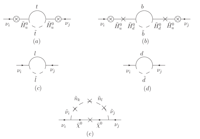
Figure 1: One loop diagrams for neutrino masses. Loops in (a), (b), (c), and (d) are induced by fermion and its superpartner. In (e) it is induced by neutralino, left- and right- chiral sneutrinos.

$$(m_{\nu}^{r})_{ij}=\frac{3y_{t}^{2}}{32\pi^{2}}\frac{m_{t}\sin 2\phi_{t}}{(m_{H_{u}^{0}})^{2}}\left\{\frac{M_{P_{2}}^{2}}{m_{t}^{2}-M_{P_{2}}^{2}}\ln\frac{m_{t}^{2}}{M_{P_{2}}^{2}}-\frac{M_{P_{1}}^{2}}{m_{t}^{2}-M_{P_{1}}^{2}}\ln\frac{m_{t}^{2}}{M_{P_{1}}^{2}}\right\}\epsilon_{i}^{\prime}\epsilon_{j}^{\prime},$$ (32)

where $\epsilon^{\prime}_{i}=Y_{\nu}^{ij}n_{j}-\epsilon_{i}$, $y_{t}$ is top Yukawa coupling, $\phi_{t}$ is the angle of left-right mixing of stop states and $M_{P_{1}},M_{P_{2}}$ are two mass eigenvalues of stops. Diagram 1(b) requires two more mass insertions plus the replacement of $y_{t}(m_{t})$ by $y_{b}(m_{b})$, causing a relative suppression. 1(c) and 1(d) also give smaller contributions [18], since they are bilinear in $\lambda_{ijk}$ and $\lambda^{\prime}_{ijk}$, which are restricted to rather small values due to the constraint on left-sneutrino vev’s [15]. And finally, diagram 1(e) depends on the value of the soft parameters $A$. However, while in reference [14] it could be as big as on the TeV scale, here the parameter is of much smaller magnitude. This is because the major contribution from this diagram in the earlier case came to be proportional to $A_{\nu}^{2}$, while $A_{\nu}\sim F_{X}/M_{P}=0$ in this case. The remaining contributions, which arise essentially from the F-terms and are proportional to the neutrino Yukawa couplings, are found to be very small. Thus the contribution from diagram 1(e), too, is of a subleading nature, and the radiative contribution to neutrino mass matrix is faithfully given by equation (25).

3.4 Analysis using the observed pattern

Our purpose is to show that the scenario proposed above has a solution space with parameters which are consistent with the proposal that all new physics in the observable sector is in the Tev scale. For this, all we do is to show a few restricted cases where consistent solutions are found.

We make the following simplification to get a diagonal mass matix for the right-handed neutrinos:

$$\kappa^{111}=\kappa^{222}=\kappa^{333}=\frac{1}{6}$$ (33)

and all other $\kappa^{ijk}=0$. We can simplify our analysis further (without losing the general nature of the conclusions) by assuming the same vev for all three right-chiral sneutrinos, namely, $n_{1}=n_{2}=n_{3}=n$. With this simplification, the total neutrino mass matrix is given by

$$m_{\nu} = m_{\nu}^{s}+m_{\nu}^{r}$$ (43)

$$= a\left(\begin{array}[]{ccc}\epsilon_{1}^{\prime}\epsilon_{1}^{\prime}&\epsilon_{1}^{\prime}\epsilon_{2}^{\prime}&\epsilon_{1}^{\prime}\epsilon_{3}^{\prime}\\ \epsilon_{2}^{\prime}\epsilon_{1}^{\prime}&\epsilon_{2}^{\prime}\epsilon_{2}^{\prime}&\epsilon_{2}^{\prime}\epsilon_{3}^{\prime}\\ \epsilon_{3}^{\prime}\epsilon_{1}^{\prime}&\epsilon_{3}^{\prime}\epsilon_{2}^{\prime}&\epsilon_{3}^{\prime}\epsilon_{3}^{\prime}\end{array}\right)-b\left(\begin{array}[]{ccc}Y_{\nu}^{11}&Y_{\nu}^{12}&Y_{\nu}^{13}\\ Y_{\nu}^{12}&Y_{\nu}^{22}&Y_{\nu}^{23}\\ Y_{\nu}^{13}&Y_{\nu}^{23}&Y_{\nu}^{33}\end{array}\right)\cdot\left(\begin{array}[]{ccc}Y_{\nu}^{11}&Y_{\nu}^{12}&Y_{\nu}^{13}\\ Y_{\nu}^{12}&Y_{\nu}^{22}&Y_{\nu}^{23}\\ Y_{\nu}^{13}&Y_{\nu}^{23}&Y_{\nu}^{33}\end{array}\right)$$

$$a = \frac{(g^{2}M_{1}+g^{\prime 2}M_{2})v_{d}^{2}}{2(-\mu^{2}M_{1}M_{2}+g^{2}\mu M_{1}v_{u}v_{d}+g^{\prime 2}\mu M_{2}v_{u}v_{d})}+$$

$$\frac{3y_{t}^{2}}{32\pi^{2}}\frac{m_{t}\sin 2\phi_{t}}{(m_{H_{u}^{0}})^{2}}\left\{\frac{M_{P_{2}}^{2}}{m_{t}^{2}-M_{P_{2}}^{2}}\ln\frac{m_{t}^{2}}{M_{P_{2}}^{2}}-\frac{M_{P_{1}}^{2}}{m_{t}^{2}-M_{P_{1}}^{2}}\ln\frac{m_{t}^{2}}{M_{P_{1}}^{2}}\right\},$$

$$b = \frac{v_{u}^{2}}{n}.$$ (44)

A focal theme of our discussion is that mixing in the neutrino sector is quite different from the quark sector; thus while the latter have (to the lowest approximation) near-diagonal Yukawa couplings, the former can have ample non-diagonality there. In order to accentuate this point, we may consider the extreme case where the $Y^{ij}_{\nu}$’s are non-vanishing only for $i\neq j$. This reduces the number of unknown variables in our equations, and makes it simpler to illustrate our points. It should, however, be remembered that this corresponds to a subset of the allowed parameter space. If the digonal $Y^{ij}_{\nu}$’s are also admitted, then a larger volume in this space will be allowed, demonstrating an even better viability of the scenario.

After substituting equation (16) into (27), we obtain the six equations given below:

$$\frac{2}{3}m_{1}+\frac{1}{3}m_{2} = a\epsilon_{1}^{\prime}\epsilon_{1}^{\prime}-b((Y_{\nu}^{12})^{2}+(Y_{\nu}^{13})^{2}),$$ (45)

$$\frac{1}{6}(m_{1}+2m_{2}+3m_{3}) = a\epsilon_{2}^{\prime}\epsilon_{2}^{\prime}-b((Y_{\nu}^{12})^{2}+(Y_{\nu}^{23})^{2}),$$ (46)

$$= a\epsilon_{3}^{\prime}\epsilon_{3}^{\prime}-b((Y_{\nu}^{13})^{2}+(Y_{\nu}^{23})^{2}),$$ (47)

$$\frac{1}{3}(-m_{1}+m_{2}) = a\epsilon_{1}^{\prime}\epsilon_{2}^{\prime}-bY_{\nu}^{13}Y_{\nu}^{23},$$ (48)

$$\frac{1}{3}(m_{1}-m_{2}) = a\epsilon_{1}^{\prime}\epsilon_{3}^{\prime}-bY_{\nu}^{12}Y_{\nu}^{23},$$ (49)

$$\frac{1}{6}(-m_{1}-2m_{2}+3m_{3}) = a\epsilon_{2}^{\prime}\epsilon_{3}^{\prime}-bY_{\nu}^{12}Y_{\nu}^{13}.$$ (50)

For fixed mass eigenvalues, the above equations can be solved for the six parameters: $\epsilon_{1}^{\prime},\epsilon_{2}^{\prime},\epsilon_{3}^{\prime},Y_{\nu}^{12},Y_{\nu}^{13},Y_{\nu}^{23}$. Using the solar neutrino data, one can use $m_{1}\simeq m_{2}$ in the lowest approximation. Thus, at zeroth order, we set the left-hand sides in equations (32) and (33) equal to zero. In that case, it is possible to choose the solutions $\epsilon_{2}^{\prime}=\epsilon_{3}^{\prime}$ and $Y_{\nu}^{12}=Y_{\nu}^{13}$ (which is consistent with maximal 23-mixing), thereby reducing the six equations to four only. Of course, we get confined to an even smaller part of the entire allowed paramters space. But our conclusions still remain quite general, there being small corrections to the solutions when the non-zero value of $\Delta m^{2}_{12}$ is inserted.

The equations in the simplified form are

$$m_{1}=m_{2}=-b(Y_{\nu}^{23})^{2},$$

$$m_{3}=a(2(\epsilon_{2}^{\prime})^{2}-(\epsilon_{1}^{\prime})^{2})-2|m_{2}|,$$

$$a\epsilon_{1}^{\prime}\epsilon_{2}^{\prime}=Y_{\nu}^{12}\sqrt{b|m_{2}|},$$

$$\frac{a^{2}}{|m_{2}|}(\epsilon_{1}^{\prime})^{4}+a\left[1+\frac{m_{3}}{|m_{2}|}\right](\epsilon_{1}^{\prime})^{2}-|m_{2}|=0.$$ (51)

where one should note that each of the first and second mass eigenvalues has Majorana phase equal to $\pi$.

From the four equations given above, we can determine the four parameters still remaining independent: $\epsilon_{1}^{\prime},\epsilon_{2}^{\prime},Y_{\nu}^{12},Y_{\nu}^{23}$. We simultaneously check that the EWSB conditions which are listed in section 2.2 are satisfied in parameter space we are led into. Some sample solutions thus obtained have been presented in the next section.

It should however, be kept in mind that we have made use of just a few hidden sector superfields in the effective low-energy theory. Therefore, the treatment described here cannot address potentially destabilising higher order effects in the final supergravity framework. Thus, the relationships among the numerical values of various parameters should be treated as indicative ones only.

We also admit that minimization of only the tree-level potential has been considered here, and the conditions are obviously going to change when loop corrections are taken into account. However, even then the general conclusion that neutrino masses and mixing can be governed by TeV scale physics, mediated via right-chiral neutrino superfields and electroweak symmetry breaking conditions, continues to be true in this sample scenario allowing $\Delta L=1$.

4 Numerical results

To solve for the four unknown parameters in equation (35), we need to know the mass eigenvalues of neutrinos. So far, we do not know the exact values of neutrino masses. From the available data, which suggest neutrino oscillations, the following mass-squared differences are favoured [32]:

$$\Delta m_{21}^{2} = (8.0\pm 0.3)\times 10^{-5}{\rm eV}^{2},$$

$$|\Delta m_{32}^{2}| = (2.5\pm 0.3)\times 10^{-3}{\rm eV}^{2}.$$ (52)

The two mass-squared differences shown above indicates three possibilities [34], namely

1. Normal hierarchy: $m_{1}\approx m_{2}\sim\sqrt{\Delta m_{21}^{2}}$, $m_{3}\sim\sqrt{|\Delta m_{32}^{2}|}$.

2. Inverted hierarchy: $m_{1}\approx m_{2}\sim\sqrt{|\Delta m_{32}^{2}|}$, $m_{3}\ll\sqrt{|\Delta m_{32}^{2}|}$.

3. Degenerate masses: $m_{1}\approx m_{2}\approx m_{3}\gg\sqrt{|\Delta m_{32}^{2}|}$.

We solve the four equations in equation (35) in each of the above three cases for the parameters $\epsilon_{1},\epsilon_{2},Y_{\nu}^{12},Y_{\nu}^{23}$. It is to be noticed that earlier we chose $\epsilon_{2}^{\prime}=\epsilon_{3}^{\prime}$ and $Y_{\nu}^{12}=Y_{\nu}^{13}$. This implies $\epsilon_{2}=\epsilon_{3}$, a postulate frequently made in bilinear R-parity violation in the light of maximal $\nu_{\mu}-\nu_{\tau}$ mixing. We plug these parameters in equation (12) to solve SUSY soft breaking parameters. Next we check in each case whether the combination of parameters ensure that EWSB is triggered by following the prescriptions of section 2.2. For simplicity, we have chosen the various SUSY soft breaking parameters to be of the form:

$$(m_{\tilde{L}}^{2})^{ij}=m_{\tilde{L}}^{2}\delta^{ij},\quad(m_{\tilde{N}}^{2})^{ij}=m_{\tilde{N}}^{2}\delta^{ij},\quad(A_{\nu}Y_{\nu})^{ij}=(A_{\nu}Y_{\nu})\delta^{ij},$$

$$(A_{\kappa}\kappa)^{ijk}=0~{}{\rm if~{}any~{}of~{}the~{}indices~{}are~{}different~{}from~{}each~{}other}.$$ (53)

These forms also ensure the suppression of FCNC. In this case one has $(A_{\kappa}\kappa)^{222}=(A_{\kappa}\kappa)^{333}$ and $(B_{\epsilon}\epsilon)^{2}=(B_{\epsilon}\epsilon)^{3}$. The numerical values of various standard model and MSSM parameters chosen for our analysis are

$$M_{2}=300~{}{\rm GeV},M_{1}=0.5M_{2},m_{t}=172.9~{}{\rm GeV},m_{H_{u}}^{2}=-(300~{}{\rm GeV})^{2},m_{\tilde{L}}^{2}=(500~{}{\rm GeV})^{2},$$

$$(A_{\nu}Y_{\nu})=10^{-4}~{}{\rm GeV},M_{P_{2}}=600~{}{\rm GeV},M_{P_{1}}=500~{}{\rm GeV},\sin 2\phi_{t}=1.$$ (54)

We present our numerical values in tabular form in each case.

4.1 Normal hierarchy

We have taken $m_{1}\approx m_{2}=\sqrt{0.8}\times 10^{-11}~{}{\rm GeV}$, $m_{3}=\sqrt{25.}\times 10^{-11}~{}{\rm GeV}$. Table 2 contains some sample solutions in this scenario.

$\tan\beta$	8.5	8.5	8.5	8.5	8.5	8.5	8.5	8.5
$m_{\tilde{N}}$	500.0	500.0	200.0	200.0	500.0	500.0	200.0	500.0
$\mu$	300.0	-300.0	300.0	-300.0	500.0	-500.0	500.0	-500.0
$n$	1000.0	1000.0	400.0	400.0	1000.0	1000.0	400.0	400.0
$\epsilon_{1}$	-0.0015	-0.0009	-0.0021	-0.0015	-0.0028	-0.0022	-0.0034	-0.0028
$\epsilon_{2}$	-0.011	-0.0079	-0.0117	-0.0086	-0.0175	-0.0145	-0.0182	-0.0152
$Y_{\nu}^{12}$
$(\times 10^{-7})$	4.147	4.147	2.623	2.623	4.147	4.147	2.623	2.623
$Y_{\nu}^{23}$
$(\times 10^{-7})$	5.473	5.473	3.461	3.461	5.473	5.473	3.461	3.461
$(B_{\mu}\mu)$	34388.7	34388.7	34388.7	34388.7	1394388.8	1394388.8	1394388.8	1394388.8
$m_{H_{d}}$	454.3	454.3	454.3	454.3	3406.8	3406.8	3406.8	3406.8
$(A_{\kappa}\kappa)^{111}$	-750.0	-750.0	-300.0	-300.0	-750.0	-750.0	-300.0	-300.0
$(A_{\kappa}\kappa)^{222}$	-750.0	-750.0	-300.0	-300.0	-750.0	-750.0	-300.0	-300.0
$(B_{\epsilon}\epsilon)^{1}$	0.432	0.576	-0.0008	0.143	0.302	0.693	-0.131	0.26
$(B_{\epsilon}\epsilon)^{2}$	0.159	0.894	-0.334	0.402	-0.504	1.491	-0.996	0.999

Table 2: Various sample solutions corresponding to normal hierarchy. All masses are in GeV.

In the table, the first four parameters such as $\tan\beta$, $m_{\tilde{N}}$, $\mu$ and $n$ are fixed in such a way as to get real solutions of equation (35) and also satisfy EWSB conditions. In order to have real solutions for $\epsilon_{1}$, $\epsilon_{2}$, $Y_{\nu}^{12}$ and $Y_{\nu}^{23}$ from equation (35), we have found that $\tan\beta$ should be at least 8.5, independent of $\mu$ and $n$. We have allowed $\mu$ to vary from $\pm$300 GeV to $\pm$500 GeV. Among the EWSB conditions, the requirement that the potential at the minima is negative puts the severest constraint on the right-handed sneutrino vev,$n$, for a particular value of $m_{\tilde{N}}$. From table 2 it can be noticed that for $m_{\tilde{N}}$ of 500, the minimum value of $n$ should be around 1000 GeV. If we decrease $m_{\tilde{N}}$ to 200, the value of $n$ should be at least 400 GeV.

This vindicates our earlier statement, based largely on the requirement of negativity of the scalar potential at the minimum, that $\langle\tilde{n}_{i}\rangle$ around the electroweak scale is viable. Even if small values of $\langle\tilde{n}_{i}\rangle$ can be engineered via fine tuning, it would bring light sterile neutrinos into the picture, taking us outside the ambit of three-flavour tri-bimaximal mixing. Such a digression is avoided in this study.

For each case one can also evaluate the various soft SUSY breaking parameters like $(B_{\mu}\mu)$, $m_{H_{d}}$, $(A_{\kappa}\kappa)^{111}$, $(A_{\kappa}\kappa)^{222}$, $(B_{\epsilon}\epsilon)^{1}$, $(B_{\epsilon}\epsilon)^{2}$, using equation (12). One should perhaps note that the $\epsilon$-parameters are of rather small values due to the restrictions on left-chiral sneutrino vev’s, a constraint arising from neutrino masses and widely used in works on R-parity violating SUSY. If we factor out such small values, the SUSY-breaking parameters including $B_{\epsilon}$ are roughly around the TeV range, as expected.

4.2 Inverted hierarchy

In this case we have taken $m_{1}\approx m_{2}=\sqrt{25.}\times 10^{-11}~{}{\rm GeV}$, $m_{3}=10^{-3}\times m_{2}$. Some sample solutions in the parameter space are presented in table 3.

$\tan\beta$	8.5	8.5	8.5	8.5	8.5	8.5	8.5	8.5
$m_{\tilde{N}}$	500.0	500.0	200.0	200.0	500.0	500.0	200.0	200.0
$\mu$	300.0	-300.0	300.0	-300.0	500.0	-500.0	500.0	-500.0
$n$	1000.0	1000.0	400.0	400.0	1000.0	1000.0	400.0	400.0
$\epsilon_{1}$	-0.009	-0.006	-0.011	-0.0078	-0.015	-0.012	-0.017	-0.014
$\epsilon_{2}$	-0.014	-0.0097	-0.0158	-0.0116	-0.0229	-0.0188	-0.0247	-0.0207
$Y_{\nu}^{12}$
$(\times 10^{-6})$	1.164	1.164	7.36	7.36	1.164	1.164	7.36	7.36
$Y_{\nu}^{23}$
$(\times 10^{-6})$	1.294	1.294	8.184	8.184	1.294	1.294	8.184	8.184
$(B_{\mu}\mu)$	34388.7	34388.7	34388.7	34388.7	1394388.8	1394388.8	1394388.8	1394388.8
$m_{H_{d}}$	454.3	454.3	454.3	454.3	3406.8	3406.8	3406.8	3406.8
$(A_{\kappa}\kappa)^{111}$	-750.0	-750.0	-300.0	-300.0	-750.0	-750.0	-300.0	-300.0
$(A_{\kappa}\kappa)^{222}$	-750.0	-750.0	-300.0	-300.0	-750.0	-750.0	-300.0	-300.0
$(B_{\epsilon}\epsilon)^{1}$	0.865	1.6	-0.241	0.454	0.239	2.124	-0.867	1.018
$(B_{\epsilon}\epsilon)^{2}$	0.748	1.76	-0.417	0.595	-0.164	2.581	-1.328	1.417

Table 3: Various sample solutions corresponding to inverted hierarchy. All masses are in GeV.

As in the case of normal hierarchy, here also we have found a minimum required value of 8.5 for $\tan\beta$ in order to get real solutions of equation (35). The condition that the potential at the minima should be less than zero puts lower limit on $n$ for a particular value of $m_{\tilde{N}}$. The least values of $n$ thus obtained have been presented in solutions, here as well as in the tables 2 and 4. Except the parameters $(B_{\mu}\mu)$, $m_{H_{d}}$, $(A_{\kappa}\kappa)^{111}$ and $(A_{\kappa}\kappa)^{222}$, all other parameters in inverted hierarchy are different from the previous case because of different neutrino mass eigenvalues.

4.3 Degenerate neutrinos

For this case we have used $m_{1}\approx m_{2}\approx m_{3}=10^{-10}~{}{\rm GeV}$. Table 4 contains some sample solutions.

$\tan\beta$	5	5	5	5	1.5	2.5	1.5	2.5
$m_{\tilde{N}}$	500.0	500.0	200.0	200.0	500.0	500.0	200.0	200.0
$\mu$	300.0	-300.0	300.0	-300.0	500.0	-500.0	500.0	-500.0
$n$	1000.0	1000.0	400.0	400.0	1000.0	1000.0	400.0	400.0
$\epsilon_{1}$	0.0006	0.0001	-0.0018	-0.0022	0.0013	-0.0094	-0.0015	-0.0118
$\epsilon_{2}$	-0.0018	-0.0026	-0.0043	-0.0052	-0.0008	-0.022	-0.0038	-0.0248
$Y_{\nu}^{12}$
$(\times 10^{-6})$	1.559	1.559	0.986	0.986	1.837	1.646	1.162	1.041
$Y_{\nu}^{23}$
$(\times 10^{-6})$	1.853	1.853	1.172	1.172	2.184	1.957	1.381	1.238
$(B_{\mu}\mu)$	19196.7	19196.7	19196.7	19196.7	242399.6	407529.8	242399.6	407529.8
$m_{H_{d}}$	99.1	99.1	99.1	99.1	339.4	878.5	339.4	878.5
$(A_{\kappa}\kappa)^{111}$	-750.0	-750.0	-300.0	-300.0	-750.0	-750.0	-300.0	-300.0
$(A_{\kappa}\kappa)^{222}$	-750.0	-750.0	-300.0	-300.0	-750.0	-750.0	-300.0	-300.0
$(B_{\epsilon}\epsilon)^{1}$	1.505	1.837	0.045	0.376	1.141	4.274	-0.57	2.735
$(B_{\epsilon}\epsilon)^{2}$	1.495	2.168	-0.098	0.574	0.494	7.034	-1.373	5.355

Table 4: Various sample solutions corresponding to degenerate neutrinos. All masses are in GeV.

Unlike the two previous cases, we have got different $\tan\beta$ values here. We have found that for $\mu=\pm$300 GeV, $\tan\beta$ should be at least 5 in order that equation (35) yields real solutions for $\epsilon_{i}$ and $Y^{ij}_{\nu}$. Moreover, for a $\mu~{}=$ 500 GeV and -500 GeV, we have found that the minimum of $\tan\beta$ should be around 1.5 and 2.5 respectively, the former of which is practicaly ruled out from the Large Electron Positron (LEP) collider data. We find that for large $\mu$, the minimum allowed value of $\tan\beta$ is sensitive to the sign of $\mu$. This kind of feature is not there in the two previous cases. The EWSB conditions give similar constraints as in the previous two cases.

5 Summary and conclusions

In this work we have studied R-parity violating effects on neutrino masses. The special features of neutrinos are postulated to arise from nonrenormalizable interactions with hidden sector fields. Proposing right-chiral Majorana-like neutrino superfields and choosing specific R-charges of hidden and visible sector superfields, we could construct a term in the superpotential, which violates lepton number by three units and thus violates R-parity explicitly.

Comparing our model with reference [14], an interesting dichotomy can be observed. Whereas non-vanishing of $F_{X}$-values have a crucial role in the previous case, they are forced to be zero here. The role has now shifted to the $\Delta L=3$ term in the superpotential, which is allowed by our R-charge assignments.

It has been further argued by us that lepton number violation, distinct R-charges for the right-chiral (s)neutrinos and special properties of the hidden sector fields they couple to — all have led together to the distinctive features of neutrino masses and mixing. After SUSY breaking and EWSB, neutrino masses of the right order are generated from seesaw and radiative effects, provided that the vev’s of right-chiral sneutrinos are of order 1 TeV. The model is also subjected to conditions arisng from EWSB. Finally, we succeed in demonstrating that viable solutions exist, with the requisite mixing pattern, for each of the cases of normal hierarchy, inverted hierarchy and degenerate neutrinos. The scheme to link features of the neutrino sector to the TeV scale, initiated in a previous work by us, is thus completed.

References

- [1] For general introductions, see, for example, H.P. Nilles, Phys. Rep. 110, 1 (1984); H.E. Haber and G.L. Kane, Phys. Rep. 117, 75 (1985); Perspectives in Supersymmetry, G. Kane (Ed.), World Scientific, Singapore (1998).
- [2] Super-Kamiokande Collaboration (S. Fukuda et al.), Phys. Rev. Lett., 85, 3999 (2000); T. Toshito (for the Super-Kamiokande Collaboration), [arXiv: hep-ex/0105023]; MACRO Collaboration (M. Ambrosio et al.), Phys. Lett. B 517, 59 (2001); MACRO Collaboration (Giorgio Giacomelli et al.), [arXiv: hep-ex/0110021]; SNO Collaboration (Q.R. Ahmad et al.), Phys. Rev. Lett. 89, 011301 (2002) [arXiv: nucl-ex/0204008]; SNO Collaboration (Q.R. Ahmad et al.), Phys. Rev. Lett. 89, 011302 (2002) [arXiv: nucl-ex/0204009]; SNO Collaboration (S.N. Ahmed et al.), Phys. Rev. Lett. 92, 181301 (2004) [arXiv: nucl-ex/0309004].
- [3] See, for example, A.Y. Smirnov, Int. J. Mod. Phys. A 19, 1180 (2004); M. Maltoni, T. Schwetz, M.A. Tortola and J.W.F. Valle, New J. Phys. 6, 122 (2004).
- [4] L. Hall, H. Murayama and N. Weiner, Phys. Rev. Lett. 84, 2572 (2000); N. Haba and H. Murayama, Phys. Rev. D 63, 053010 (2001); G. Altarelli, F. Feruglio and I. Masina, J. High Energy Phys. 0301, 035 (2003).
- [5] E. Ma and G. Rajasekaran, Phys. Rev. D 64, 113012 (2001); E. Ma, Phys. Rev. D 70, 031901(R) (2004); E. Ma, New J. Phys. 6, 104 (2004); G. Altarelli and F. Feruglio, Nucl. Phys. B720, 64 (2005).
- [6] K.S. Babu, E. Ma and J.W.F. Valle, Phys. Lett. B 552, 207 (2003).
- [7] S. Davidson and S.F. King, Phys. Lett. B 445, 191 (1998).
- [8] C.S. Aulakh and R.N. Mohapatra, Phys. Lett. B 119, 136 (1982); Phys. Lett. B 121, 147 (1983); K.S. Babu and R.N. Mohapatra, Phys. Rev. Lett. 83, 2522 (1999); H.S. Goh, R.N. Mohapatra and S. Ng, Phys. Lett. B 570, 215 (2003); Phys. Rev. D 68, 115008 (2003); H.S. Goh, R.N. Mohapatra, S. Nasri, S. Ng, Phys. Lett. B 587, 105 (2004).
- [9] B. Mukhopadhyaya, Proc. Indian Natl. Sci. Acad. 70A, 239 (2004) [arXiv: hep-ph/0301278], and references therein.
- [10] N. Arkani-Hamed, L. Hall, H. Murayama, D. Smith and N. Weiner, Phys. Rev. D 64, 115011 (2001).
- [11] N. Arkani-Hamed, L. Hall, H. Murayama, D. Smith and N. Weiner, [arXiv: hep-ph/0007001].
- [12] F. Borzumati and Y. Nomura, Phys. Rev. D 64, 053005 (2001); F. Borzumati, K. Hamaguchi and T. Yanagida, Phys. Lett. B 497, 259 (2001).
- [13] K.S. Babu and T. Yanagida, Phys. Lett. B 491, 148 (2000).
- [14] B. Mukhopadhyaya, P. Roy and R. Srikanth, Phys. Rev. D 73, 035003 (2006), [arXiv: hep-ph/0510298].
- [15] S. Roy and B. Mukhopadhyaya, Phys. Rev. D 55, 7020 (1997).
- [16] B. Mukhopadhyaya and S. Roy and F. Vissani, Phys. Lett. B 443, 191 (1998).
- [17] A. Datta, B. Mukhopadhyaya and S. Roy, Phys. Rev. D 61, 055006 (2000).
- [18] Y. Grossman and H.E. Haber, Phys. Rev. D 59, 093008 (1999).
- [19] J. Ferrandis, Phys. Rev. D 60, 095012 (1999).
- [20] S. Bar-Shalom, G. Eilam and B. Mele, Phys. Rev. D 64, 095008 (2001).
- [21] J.W.F. Valle, [arXiv: hep-ph/9808292]; M. Hirsh, M.A. Diaz, W. Porod, J.C. Romao and J.W.F. Valle, Phys. Rev. D 62, 113008 (2000); M.A. Diaz, M. Hirsh, W. Porod, J.C. Romao and J.W.F. Valle, Phys. Rev. D 68, 013009 (2003); M. Hirsh, J.W.F. Valle, New J. Phys. 6, 76 (2004).
- [22] D.E. Lopez-Fogliani and C.Munoz, [arXiv: hep-ph/0508297].
- [23] M. Bisset, O.C.W. Kong, C. Macesanu and L.H. Orr, Phys. Lett. B 430, 274 (1998); Phys. Rev. D 62, 035001 (2000); O.C.W. Kong, Mod. Phys. Lett. A 14, 903 (1999); C. Chang, T. Feng and L. Shan, Commun. Theor. Phys. 33, 421 (2000); T. Feng, [arXiv: hep-ph/9808379]; E.J. Chun, S.K. Kang, C.W. Kim and U.W. Lee, Nucl. Phys. B544, 89 (1999); E.J. Chun and J.S. Lee, Phys. Rev. D 60, 075006 (1999).
- [24] A.S. Joshipura and M. Nowakowski, Phys. Rev. D 51, 2421 (1995); M. Drees, S. Pakvasa, X. Tata and T. ter Veldhuis, Phys. Rev. D 57, 5335 (1998); A.S. Joshipura, R.D. Vaidya and S.K. Vempati, Nucl. Phys. B639, 290 (2002).
- [25] S. Rakshit, G. Bhattacharyya and A. Raychaudhuri, Phys. Rev. D 59, 091701 (1999).
- [26] G.F. Giudice and A. Masiero, Phys. Lett. B 206, 480 (1988); J.A. Casas and C. Munoz, Phys. Lett. B 306, 288 (1993); L.J. Hall, Y. Nomura and A. Pierce, Phys. Lett. B 538, 359 (2002).
- [27] S. Davidson, Phys. Lett. B 439, 63 (1998).
- [28] V.D. Barger, G.F. Giudice and T. Han, Phys. Rev. D 40, 2987 (1989).
- [29] J.F. Gunion and H.E. Haber, Nucl. Phys. B272, 1 (1986); I. Simonsen, [arXiv: hep-ph/9506369].
- [30] S. Eidelman, et al., Phys. Lett. B 592, 1 (2004).
- [31] See references in [2]. M. Apollonio et al., Phys. Lett. B 466, 415 (1999); K. Eguchi et al. (KamLand Collaboration), Phys. Rev. Lett. 90, 021802 (2003); A. Bandyopadhyay, S. Choubey, S. Goswami, S.T. Petcov and D.P. Roy, Phys. Lett. B 583, 134 (2004); P.C. Holanda and A.Yu. Smirnov, Astropart. Phys. 21, 287 (2004); G.L. Fogli et al., Phys. Rev. D 69, 017301 (2004); M. Maltoni, T. Schwetz, M.A. Tortola and J,W.F. Valle, New J. Phys. 6, 122 (2004).
- [32] A. Strumia and F. Vissani, Nucl. Phys. B726, 294 (2005).
- [33] P.F. Harrison, D.H. Perkins and W.G. Scott, Phys. Lett. B 530, 167 (2002).
- [34] E. Ma, Phys. Rev. D 66, 117301 (2002); A. Joshipura, Proc. Indian Natl. Sci. Acad. 70A, 223 (2004).