hep-ph/0605100
IISc-CHEP/4/06, LPT-ORSAY-06-32  

Lepton distribution as a probe of new physics in production and decay of the $t$ quark and its polarization

Rohini M. Godbole ^a,1, Saurabh D. Rindani ^b,2, Ritesh K. Singh ^c,3
aCenter for High Energy Physics, IISc, Bangalore, 560 012, INDIA

^bPhysical Research Laboratory, Navarangpura, Ahmedabad 380 009, INDIA

^cLaboratoire de Physique Théorique, 91405 Orsay Cedex, FRANCE

¹rohini@cts.iisc.ernet.in, ²saurabh@prl.res.in, ³ritesh.singh@th.u-psud.fr

Abstract
We investigate the possibility of studying new physics in various processes of $t$-quark production using kinematical distributions of the secondary lepton coming from the decay of $t$ quarks. We show that the angular distribution of the secondary lepton is insensitive to the anomalous $tbW$ vertex and hence is a pure probe of new physics in a generic process of $t$-quark production. The energy distribution of the lepton is distinctly affected by anomalous $tbW$ couplings and can be used to analyze them independent of the production process of $t$ quarks. The effects of $t$ polarization on the distributions of the decay lepton are demonstrated for top-pair production process at a $\gamma\gamma$ collider mediated by a heavy Higgs boson.

PACS number(s) : 14.65.Ha, 13.88.+e, 13.85.Qk
Keywords :top, polarization, anomalous top coupling
 

 

1 Introduction

The mechanism of spontaneous symmetry breaking (SSB), which is responsible for generating masses for all fermions and weak bosons, still lacks explicit experimental verification. In the Standard Model (SM), Higgs mechanism is responsible for the SSB and the Higgs boson, being a remnant degree of freedom after symmetry breaking, carries information about the phenomenon of symmetry breaking. The top quark, whose mass is very close to the electroweak symmetry breaking scale, is expected to provide a probe for understanding SSB in the SM. Direct experimental observation of the Higgs boson is essential for establishing the Higgs mechanism as the correct SSB mechanism.

The SM has been tested to be the model of particle interactions for all the particles other than the $t$ quark, which has not yet been studied extensively at the colliders and the Higgs boson, which is yet to be observed experimentally. In addition to the discovery of the Higgs boson, it is also essential to measure accurately the couplings of the Higgs boson and the top quark to other SM particles with high precision. If these couplings would be found to be the same as those predicted in the SM then it will confirm the Higgs mechanism of SSB. Any deviation will signal presence of physics beyond the SM.

In spite of the impressive agreement of all the precision electroweak (EW) measurements with the predictions of the SM, it still suffers from quite a few deficiencies from a theoretical point of view. For example, the mass of the SM Higgs boson is not stable against radiative corrections; also the SM does not provide a first principle understanding of the phenomenon of $CP$ violation, even though it does contain a successful parametrization of the same in terms of the CKM phase, etc. All attempts to cure these and other ills of the SM require us to go beyond the SM. Such physics beyond the SM will imply deviations of the couplings of the Higgs boson and the top quark with each other as well as with other SM particles. The specific deviations of the top quark couplings from the expectations of the SM may depend on the details of the particular extension of the SM one is looking at. In this work, we adopt a model-independent formulation and allow, in the effective theory approach, the most general interaction of $t$ with other SM particles. For example, the most general expression for the $tbW$ vertex may be written as,

$$\Gamma^{\mu} = \frac{-ig}{\sqrt{2}}\ \left[\gamma^{\mu}(f_{1L}P_{L}+f_{1R}P_{R})-\frac{i\sigma^{\mu\nu}}{m_{W}}\ (p_{t}-p_{b})_{\nu}\ (f_{2L}P_{L}+f_{2R}P_{R})\right].$$ (1)

For the SM, $f_{1L}=1$ and the anomalous couplings $f_{1R}=f_{2L}=f_{2R}=0$. The various extensions of the SM would have specific predictions for these anomalous couplings. Since in a renormalizable theory, these can arise only at a higher order in perturbation theory, we assume them to be small and retain only terms linear in them. The couplings of the $t$ quark with other gauge bosons can also be parametrized in a model-independent way similar to Eq. (1).

These non-standard couplings may give rise to changes in the kinematical distributions and polarization of the produced $t$ quarks. Kinematic distributions of the decay products of the polarized top quark can yield information on its polarization and can be used to construct probes of the anomalous top-quark couplings involved in their production. Such analysis is simplified if one can devise observables which are sensitive only to the anomalous coupling involved in the production process and are independent of a possible anomalous $tbW$ vertex. We call these observables decoupled observables. Such observables when used in conjunction with the remaining observables may be also yield information about the anomalous $tbW$ vertex itself. The angular distribution of the secondary lepton coming from the decay of the $t$ quark is a decoupled observable. The energy distribution of the secondary lepton, on the other hand, depends upon the anomalous $tbW$ couplings along with possible new physics in the production of the $t$ quark. The angular distribution of the $b$ quark from the decay of the $t$ quark is also sensitive to the $t$ polarization as well as to the anomalous $tbW$ vertex. Note that the angular distribution of the decay lepton in the rest frame of the $t$ quark involves only the polarization of the parent quark.

The independence of the lepton angular distribution from the anomalous $tbW$ coupling has been observed for $e^{+}e^{-}\to t\bar{t}$ [1, 2] and $\gamma\gamma\to t\bar{t}$ [3, 4] earlier, neglecting the $b$ quark mass. It has been shown that such a result holds independent of the initial state [5] for a massless $b$ quark and also applies to any inclusive $t$-quark production process for a massive $b$ quark [6]. This possibility gives us a tool to study any non-SM physics involved in $t$-quark production at all colliders. In this paper we extend our earlier analysis [1, 4] to $2\to n$ reactions with more relaxed assumptions on the kinematics and discuss the use of lepton distributions in reconstructing the polarization of the $t$ quark in a generic production process.

Polarization of the $t$ quark is a good probe of new physics beyond the SM including $CP$ violation. It can be estimated using the shape of the distributions of its decay products [7, 8, 9, 10, 11] or the polarization of the $W$ [12, 13, 14]. Recently, a more realistic study of top quark spin measurement has been performed [15] using a newly devised method [16]. Top polarization in the SM has been studied in great detail: at tree level in [17, 18], including electroweak corrections in [19, 20], including QCD corrections in [21, 22] and including electroweak as well as QCD corrections in [23, 24]. Further, threshold effects in $t\bar{t}$ production and top polarization have been studied within the framework of the SM in Refs. [25, 26, 27, 28, 29, 30]. Spin correlations in top pair production have been studied [31, 32, 33, 34, 35]. QCD corrections to such correlations have also been studied [36, 37, 38, 39, 40, 41, 42, 43].

In this paper we study the polarization of the $t$ quark in a generic production process, which may receive contributions from new physics, using kinematical distributions of secondary leptons, as well as those of $b$ quarks. We also consider the possibility of probing the new physics contribution to top production and decay separately.

Our main results may be summarized as follows. The lepton angular distribution is shown to be completely insensitive to any anomalous $tbW$ coupling assuming a narrow-width approximation for the $t$ quark and keeping only terms linear in anomalous $tbW$ couplings for any top-production process. The decay lepton energy distribution in the rest frame of the $t$ quark, on the other hand, is sensitive only to the anomalous $tbW$ couplings. Specific asymmetries involving lepton angular distribution relative to the top momentum can be constructed which measure the top polarization in a generic process of $t$-quark production.

The rest of the paper is organized as follows. In Section 2 we generalize the decoupling theorem for non-zero mass of the $b$ quark and keeping all the anomalous couplings in Eq. (1) non-zero. We identify the main ingredients in arriving at the decoupling theorem and in Section 3 we extend it to a generic $2\to n$ process of $t$-quark production. We also discuss the effect of the inclusion of radiative corrections in our analysis on the validity of this decoupling theorem. In Section 4 we construct lepton angular asymmetries to reconstruct the polarization density matrix of the decaying $t$ for any generic process. In Section 5 we use the energy distribution of the secondary lepton to probe anomalous $tbW$ couplings and also discuss the possibility of probing $t$ polarization using $E_{\ell}$ distributions. In Section 6, we demonstrate the effects of $t$ polarization on the angular distribution of the decay leptons from the $t$ quark produced in the process $\gamma\gamma\to t\bar{t}$, where the production also includes contribution coming from the Higgs-boson mediated diagram. Section 7 discusses the use of the $b$-quark angular distribution in conjunction with the lepton angular distribution as a probe of anomalous $tbW$ vertex. We discuss our results in Section 8 and conclude.

2 Angular distribution of secondary leptons in $A\ B\to t\ \bar{t}$

We first look at $t\bar{t}$ production at either an $e^{+}e^{-}$ or a $\gamma\gamma$ collider followed by the decay of $t/\bar{t}$ into secondary leptons. We take the most general $tbW$ vertex. The process is shown in Fig 1.

Figure 1: The diagram depicting generic $2\to 2$ process of $t$-quark pair production and subsequent decays.

The square of the matrix element for this process, including semi-leptonic decay of $t$ and inclusive decay of $\bar{t}$, can be written using the narrow width approximation for the $t$ quark as

$$\overline{|{\cal M}|^{2}}=\frac{\pi\delta(p_{t}^{2}-m_{t}^{2})}{\Gamma_{t}m_{t}}\sum_{\lambda,\lambda^{\prime}}\rho(\lambda,\lambda^{\prime})\Gamma(\lambda,\lambda^{\prime}).$$ (2)

Here we have

$$\rho(\lambda,\lambda^{\prime})=M_{\rho}(\lambda)\ M^{*}_{\rho}(\lambda^{\prime})\hskip 14.22636pt\mbox{and}\hskip 14.22636pt\Gamma(\lambda,\lambda^{\prime})=M_{\Gamma}(\lambda)\ M^{*}_{\Gamma}(\lambda^{\prime}),$$ (3)

where $M_{\rho}(\lambda)$ is the production amplitude of a $t$ quark with helicity $\lambda$, and $M_{\Gamma}(\lambda)$ is the decay matrix element of a $t$ quark with helicity $\lambda$. We study the process $A+B\to\bar{t}b\nu\ell^{+}$ where the $\bar{t}$ decays inclusively. The differential cross-section for this process can be written as

$$d\sigma=\frac{(2\pi)^{4}}{2I}\ \overline{|{\cal M}|^{2}}\ \delta^{4}(k_{A}+k_{B}-p_{\bar{t}}-p_{b}-p_{\nu}-p_{\ell})\ \frac{d^{3}p_{\bar{t}}}{2E_{\bar{t}}(2\pi)^{3}}\ \frac{d^{3}p_{b}}{2E_{b}(2\pi)^{3}}\ \frac{d^{3}p_{\nu}}{2E_{\nu}(2\pi)^{3}}\ \frac{d^{3}p_{\ell}}{2E_{\ell}(2\pi)^{3}},$$ (4)

where $I^{2}=[s-(m_{A}+m_{B})^{2}][s-(m_{A}-m_{B})^{2}]$. Using the expression for $\overline{|{\cal M}|^{2}}$ and inserting

$$1=\intop d^{4}p_{t}\delta^{4}(p_{t}-p_{b}-p_{\nu}-p_{\ell})=\intop d(p_{0}^{2})\frac{d^{3}p_{t}}{2p_{0}}\ \theta(p_{0}^{2})\ \delta^{4}(p_{t}-p_{b}-p_{\nu}-p_{\ell})$$ (5)

in Eq. (4), we can rewrite the differential cross-section after integrating over $p_{0}^{2}$ as

$$d\sigma = \sum_{\lambda,\lambda^{\prime}}\left[\frac{(2\pi)^{4}}{2I}\rho(\lambda,\lambda^{\prime})\delta^{4}(k_{A}+k_{B}-p_{\bar{t}}-p_{t})\frac{d^{3}p_{\bar{t}}}{2E_{\bar{t}}(2\pi)^{3}}\ \frac{d^{3}p_{t}}{2E_{t}(2\pi)^{3}}\right]$$ (6)

$$\times \left[\frac{1}{\Gamma_{t}}\ \left(\frac{(2\pi)^{4}}{2m_{t}}\Gamma(\lambda,\lambda^{\prime})\delta^{4}(p_{t}-p_{b}-p_{\nu}-p_{\ell})\frac{d^{3}p_{b}}{2E_{b}(2\pi)^{3}}\ \frac{d^{3}p_{\nu}}{2E_{\nu}(2\pi)^{3}}\right)\frac{d^{3}p_{\ell}}{2E_{\ell}(2\pi)^{3}}\right].$$

The narrow-width approximation for the $t$ quark plays a crucial role in arriving at Eq. (6), where the differential cross-section for the full process is expressed as the product of the differential cross-section for $t\bar{t}$ production and the differential decay rate of the $t$ quark. The term in the first pair of square brackets in Eq. (6) can be written as

$$\intop\frac{d^{3}p_{\bar{t}}}{2E_{\bar{t}}(2\pi)^{3}}\ \frac{d^{3}p_{t}}{2E_{t}(2\pi)^{3}}\ \frac{(2\pi)^{4}}{2I}\ \rho(\lambda,\lambda^{\prime})\ \delta^{4}(k_{A}+k_{B}-p_{\bar{t}}-p_{t})=d\sigma_{2\to 2}(\lambda,\lambda^{\prime})d\cos\theta_{t}\ .$$ (7)

Similarly, the term in the second square bracket in Eq. (6) can be integrated in the rest frame of the $t$ quark to give

$$\frac{1}{\Gamma_{t}}\ \frac{(2\pi)^{4}}{2m_{t}}\intop\frac{d^{3}p_{\ell}}{2E_{\ell}(2\pi)^{3}}\ \ \frac{d^{3}p_{b}}{2E_{b}(2\pi)^{3}}\ \frac{d^{3}p_{\nu}}{2E_{\nu}(2\pi)^{3}}\ \ \Gamma(\lambda,\lambda^{\prime})\delta^{4}(p_{t}-p_{b}-p_{\nu}-p_{\ell})$$ (8)

$$= \frac{1}{\Gamma_{t}}\ \frac{(2\pi)^{4}}{2m_{t}}\intop\frac{d^{3}p_{\ell}}{2E_{\ell}(2\pi)^{3}}\ \ dE_{b}\ d\phi_{b}\ \ \frac{1}{4\ E_{\ell}}\frac{1}{(2\pi)^{6}}\Gamma(\lambda,\lambda^{\prime})$$

$$= \frac{1}{32\Gamma_{t}m_{t}}\ \frac{E_{\ell}}{(2\pi)^{4}}\frac{\langle\Gamma(\lambda,\lambda^{\prime})\rangle}{m_{t}E_{\ell}}\ \ dE_{\ell}\ d\Omega_{\ell}\ dp_{W}^{2}\ .$$

Here angular brackets denote an average over the azimuthal angle of the $b$ quark w.r.t the plane of the $t$ and the $\ell$ momenta chosen as the $x-z$ plane, where the $z$ axis points in the direction of the lepton momentum. We first change the angular variables of the $b$ quark from $[\cos\theta_{b},\ \phi_{b}]$ to $[\cos\theta_{b\ell},\ \phi_{b\ell}]$ and then average over $\phi_{b\ell}$. Further, the integral over $E_{b}$ is replaced by an integral over the invariant mass of the $W$ boson, $p_{W}^{2}$. Boosting the above expressions to the c.m. frame one can rewrite Eq.(6) as

$$d\sigma=\frac{1}{32\ \Gamma_{t}m_{t}}\ \frac{E_{\ell}}{(2\pi)^{4}}\left[\sum_{\lambda,\lambda^{\prime}}d\sigma_{2\to 2}(\lambda,\lambda^{\prime})\ \times\ \left(\frac{\langle\Gamma^{\prime}(\lambda,\lambda^{\prime})\rangle}{m_{t}E_{\ell}^{0}}\right)_{\rm c.m.}\right]\ d\cos\theta_{t}\ dE_{\ell}\ d\cos\theta_{\ell}\ d\phi_{\ell}\ dp_{W}^{2},$$ (9)

where $E^{0}_{\ell}$ is the lepton energy in the rest frame of the $t$ quark.

In the rest frame of the $t$ quark with the $z$ axis along the direction of the boost of the $t$ quark to the lab frame, and the $x-z$ plane coincident with the $x-z$ plane of the lab frame, the expressions for $\langle\Gamma(\lambda,\lambda^{\prime})\rangle$ are given by

$$\langle\Gamma(\pm,\pm)\rangle = g^{4}m_{t}E_{\ell}^{0}|\Delta_{W}(p_{W}^{2})|^{2}\ (1\pm\cos\theta_{l})\ \times\ F(E_{\ell}^{0}),$$

$$\langle\Gamma(\pm,\mp)\rangle = g^{4}m_{t}E_{\ell}^{0}|\Delta_{W}(p_{W}^{2})|^{2}\ (\sin\theta_{l}e^{\pm i\phi_{l}})\ \times\ F(E_{\ell}^{0}).$$ (10)

Here $\Delta(p_{W}^{2})$ is the $W$-boson propagator and $F(E_{\ell}^{0})$ is given by

$$F(E_{\ell}^{0}) = \left[(m_{t}^{2}-m_{b}^{2}-2p_{t}\cdot p_{l})\left(|f_{1L}|^{2}+\Re(f_{1L}f_{2R}^{*})\frac{m_{t}}{m_{W}}\frac{p_{W}^{2}}{p_{t}.p_{l}}\right)\right.$$ (11)

$$- \left.2\Re(f_{1L}f_{2L}^{*})\ \frac{m_{b}}{m_{W}}\ p_{W}^{2}-\Re(f_{1L}f_{1R}^{*})\ \frac{m_{b}\ m_{t}}{p_{t}.p_{l}}\ p_{W}^{2}\right].$$

Eq. (10) assumes that all the anomalous $tbW$ couplings other than $f_{1L}$ are small, and terms quadratic in them are dropped. The azimuthal correlation between $b$ and $\ell$ is sensitive to the anomalous $tbW$ couplings. The averaging eliminates any such dependence and we get $\langle\Gamma(\lambda,\lambda^{\prime})\rangle$ factorized into angular part $A(\lambda,\lambda^{\prime})$ and energy dependent part $F(E_{\ell}^{0})$. In short the expression for decay density matrix can be written as

$$\langle\Gamma(\lambda,\lambda^{\prime})\rangle=(m_{t}E_{\ell}^{0})\ |\Delta(p_{W}^{2})|^{2}\ g^{4}A(\lambda,\lambda^{\prime})\ F(E_{\ell}^{0}).$$ (12)

Here $A(\lambda,\lambda^{\prime})$ depends only on the polar and azimuthal angles of $\ell$ in the rest frame of $t$ and $F(E_{l}^{0})$ depends only on the lepton energy, various masses and couplings. After boosting to the c.m. or lab frame, they pick up additional dependence on $E_{t}$ and $\theta_{t}$. The most important point is that $\langle\Gamma(\lambda,\lambda^{\prime})\rangle$ factorizes into a pure angular part, $A(\lambda,\lambda^{\prime})$, and a pure energy dependent part, $F(E_{\ell})$. Thus the angular dependence of the density matrix remains insensitive to the anomalous $tbW$ couplings up to an overall factor $F(E_{\ell})$. Putting the expression for the decay density matrix in Eq. (6) we get

$$d\sigma = \frac{1}{32\ \Gamma_{t}m_{t}}\ \frac{1}{(2\pi)^{4}}\left[\sum_{\lambda,\lambda^{\prime}}d\sigma_{2\to 2}(\lambda,\lambda^{\prime})\ \times\ g^{4}A(\lambda,\lambda^{\prime})\right]\ d\cos\theta_{t}\ d\cos\theta_{\ell}\ d\phi_{\ell}$$ (13)

$$\times E_{\ell}\ F(E_{\ell})\ dE_{\ell}\ \ dp_{W}^{2}.$$

Since the $E_{\ell}$-dependent part has factored out, one can integrate this out. The limits of integration for $E_{\ell}$ in the c.m. frame are given by

$$\frac{p_{W}^{2}}{2E_{t}}\frac{1}{1-\beta_{t}\cos\theta_{t\ell}}\leq E_{\ell}\leq\frac{m_{t}^{2}-m_{b}^{2}}{2E_{t}}\frac{1}{1-\beta_{t}\cos\theta_{t\ell}}\ ,$$

and after integration we get

$$\int dE_{\ell}\ E_{\ell}F(E_{\ell})=\frac{1}{E_{t}^{2}\ (1-\beta_{t}\ \cos\theta_{t\ell})^{2}}\Bigg{[}-\frac{|f_{1L}|^{2}}{12}\ \bigg{(}(m_{t}^{2}-m_{b}^{2})^{3}-(p_{W}^{2})^{3}\bigg{)}$$

$$+\Bigg{(}|f_{1L}|^{2}(m_{t}^{2}-m_{b}^{2})-2\Re(f_{1L}f_{2R}^{*})\frac{m_{t}p_{W}^{2}}{m_{W}}-2\Re(f_{1L}f_{2L}^{*})\frac{m_{b}p_{W}^{2}}{m_{W}}\Bigg{)}\frac{(m_{t}^{2}-m_{b}^{2})^{2}-(p_{W}^{2})^{2}}{8}$$

$$+\Bigg{(}(m_{t}^{2}-m_{b}^{2})\Re(f_{1L}f_{2R}^{*})\frac{m_{t}p_{W}^{2}}{m_{W}}-\Re(f_{1L}f_{1R}^{*})m_{b}m_{t}p_{W}^{2}\Bigg{)}(m_{t}^{2}-m_{b}^{2}-p_{W}^{2})\Bigg{]}$$ (14)

$$=\frac{G(\{m_{i}\},\{f_{i}\},p_{W}^{2})}{E_{t}^{2}\ (1-\beta_{t}\cos\theta_{t\ell})^{2}}.$$ (15)

Here $G$ depends upon masses $\{m_{i}\}$, couplings $\{f_{i}\}$ and $p_{W}^{2}$. The same factor $G$ appears in the expression for the decay width $\Gamma_{t}$ as well, and cancels in Eq. (13) after integration over $p_{W}^{2}$, leaving the differential rate independent of any anomalous $tbW$ vertex. This decoupling of lepton distribution from the anomalous $tbW$ couplings has been shown using the same method in Ref. [4] for massless $b$ quarks for the case of $\gamma\gamma\to t\bar{t}$. Here we extend the decoupling result to include (1) a massive $b$ quark, (2) all the anomalous $tbW$ couplings and (3) finite width of the $W$ boson. The important approximations/assumptions in arriving at this result are :

1. Narrow-width approximation for the $t$ quark.

2. Smallness of $f_{1R},\ f_{2L}$ and $f_{2R}$.

3. $t\to bW(\nu\ell)$ as the only decay channel of the $t$ quark.

The first of these, viz., the narrow-width approximation for the $t$ quark, is used to factorize the differential cross-section into the production and the decay of the $t$ quark as shown in Eq. (6). The effect of the finite-width corrections on normalized distributions of the decay products is expected to be negligible. An example of explicit verification of the fact can be found in Ref. [44]. The second assumption, i.e. the smallness of the anomalous couplings is essential for the factorization of $\langle\Gamma(\lambda,\lambda^{\prime})\rangle$ into a purely angular and a purely energy-dependent part. If the lepton spectrum is calculated keeping the quadratic terms, as would be necessary for large couplings, no factorization of $\langle\Gamma(\lambda,\lambda^{\prime})\rangle$ is observed [45].

The third assumption is necessary for exact cancellation of $G$ in the numerator and $\Gamma_{t}$. If there are other decay modes of the $t$ quark than $bW$, then it will result in an extra factor of branching ratio, which is an overall constant depending upon anomalous coupling. This still maintains the decoupling of angular distribution of leptons up to an overall scale. We see that the first two assumptions are the only ones essential to achieving the decoupling while the last one only simplifies the calculation. After factorization of the differential rates into production and decay parts, the most important ingredient in achieving decoupling is the factorization of $\langle\Gamma(\lambda,\lambda^{\prime})\rangle$ into a purely angular part and a purely energy-dependent part, with the angular part being independent of any anomalous $tbW$ coupling. This factorization is achieved by averaging over the azimuthal angle of $b$ quarks and keeping only the linear terms in the anomalous $tbW$ couplings. Thus, as long as the anomalous $tbW$ couplings are small and we do not look for any correlation between azimuthal angles of $\ell$ and $b$, the lepton angular distributions remain insensitive to (or decoupled from) any anomalous $tbW$ couplings.

3 Angular distribution of secondary leptons in $A\ B\to t\ P_{1}\ ...\ P_{n-1}$

After identifying the requisites to arriving at the decoupling of the lepton distribution from an anomalous $tbW$ vertex, we intend to look at the production of the $t$ quark in a generic process $AB\rightarrow tP_{1}P_{2}..P_{n}$, followed by its semi-leptonic decay. In this section we assume only the narrow-width approximation for $t$ quarks and smallness of the anomalous $tbW$ couplings. A representative diagram of the process is shown in Fig. 2.

Figure 2: Diagram depicting $2\to n$ process

The final state particles $P_{i}$ may decay inclusively. After using the narrow-width approximation for the $t$ quark, the expression for the differential cross-section, similar to Eq. (6), can be written as :

$$d\sigma = \sum_{\lambda,\lambda^{\prime}}\left[\frac{(2\pi)^{4}}{2I}\rho(\lambda,\lambda^{\prime})\delta^{4}\bigg{(}k_{A}+k_{B}-p_{t}-\bigg{(}\sum_{i}^{n-1}p_{i}\bigg{)}\bigg{)}\frac{d^{3}p_{t}}{2E_{t}(2\pi)^{3}}\ \prod_{i}^{n-1}\frac{d^{3}p_{i}}{2E_{i}(2\pi)^{3}}\right]$$ (16)

$$\times \left[\frac{1}{\Gamma_{t}}\ \frac{(2\pi)^{4}}{2m_{t}}\Gamma(\lambda,\lambda^{\prime})\delta^{4}(p_{t}-p_{b}-p_{\nu}-p_{\ell})\frac{d^{3}p_{b}}{2E_{b}(2\pi)^{3}}\ \frac{d^{3}p_{\nu}}{2E_{\nu}(2\pi)^{3}}\frac{d^{3}p_{\ell}}{2E_{\ell}(2\pi)^{3}}\right].$$

In the c.m. frame we choose a set of axes such that the production plane of the $t$ quark defines the azimuthal reference $\phi=0$ and rewrite the production part as

$$\intop\frac{d^{3}p_{t}}{2E_{t}(2\pi)^{3}}\ \prod_{i}^{n-1}\frac{d^{3}p_{i}}{2E_{i}(2\pi)^{3}}\ \ \frac{(2\pi)^{4}}{2I}\rho(\lambda,\lambda^{\prime})\delta^{4}\bigg{(}k_{A}+k_{B}-p_{t}-\bigg{(}\sum_{i}^{n-1}p_{i}\bigg{)}\bigg{)}=d\sigma_{2\to n}(\lambda,\lambda^{\prime})\ dE_{t}d\cos\theta_{t}.$$ (17)

We will continue to use the symbol $d\sigma_{2\to n}(\lambda,\lambda^{\prime})$ independent of whether the above integral can be done in a closed form or has to be done numerically. Using this we write the expression for $d\sigma$ similar to Eq. (13) as

$$d\sigma = \frac{1}{32\ \Gamma_{t}m_{t}(2\pi)^{4}}\left[\sum_{\lambda,\lambda^{\prime}}d\sigma_{2\to n}(\lambda,\lambda^{\prime})\ \times\ g^{4}A(\lambda,\lambda^{\prime})\right]\ dE_{t}\ d\cos\theta_{t}\ d\cos\theta_{\ell}\ d\phi_{\ell}$$ (18)

$$\times E_{\ell}\ F(E_{\ell})\ dE_{\ell}\ dp_{W}^{2}.$$

Again, the $E_{\ell}$ integration will give the same factor as that appearing in the expression for $\Gamma_{t}$ which will cancel between the numerator and denominator as in the case of $2\to 2$ process of $t$-quark production. Thus we have demonstrated the decoupling of angular distribution of the leptons from anomalous $tbW$ couplings for a most general $2\to n$ production process for the $t$ quark. Any observable constructed using the angular variables of the secondary lepton will thus be completely independent of the anomalous $tbW$ vertex. Hence it is a pure probe of couplings involved in the corresponding production process and the effect of any anomalous coupling in decay process has been filtered out by averaging over the azimuthal angle of the $b$ quark and the energy of the decay leptons. Further, for hadronic decay of the $t$ quark $W\to u\bar{d}$, where $u$ stands for $u$ and $c$ quarks, and $d$ stands for $d$ and $s$ quarks, the decoupling goes through. The role of $\ell$ is taken by down-type quarks, the $T_{3}=-1/2$ fermions in the $SU(2)$ doublet. For construction of these angular distributions one needs to distinguish the $\bar{d}$-jet from the $u$-jet, which requires charge determination of light quarks. This, unfortunately, is not possible. Thus, though $\bar{d}$-jet provides a high-statistics decoupled angular distribution, it cannot be used and in real experiments we have access only to the lepton angular distribution.

The angular distribution of leptons has been used to probe new physics in various processes of $t\bar{t}$ production at a Linear Collider [46] and a photon collider [47]. All of these studies had assumed a massless $b$ quark and hence included the effect only of $f_{2R}$ from the anomalous part of the $tbW$ vertex. With the above proof of decoupling, now all the results of Ref. [46, 47] can be extended to include the case of a massive $b$ quark, and thus the case of all the anomalous $tbW$ couplings being nonzero.

This decoupling has been demonstrated only after averaging over the entire allowed range of the lepton energy. One might worry that an experiment will always involve a lower cut on the energy $E_{\ell}^{lab}$ of the lepton in the laboratory frame which may be higher than the minimum $E_{\ell}^{lab}$ allowed kinematically. In fact for $t$ quarks with velocity $\sim 0.7\ c$ in the laboratory frame, the minimum value of $E_{\ell}^{lab}$ is about 8 GeV and thus a cut will cause no problem for the validity of the decoupling. In our numerical analysis for the chosen collider energy, the minimum energy of the lepton in the laboratory is always above the typical energy cut.

Radiative corrections : We now examine to what extent the general proof of the decoupling of the lepton angular distribution for $2\to n$ process goes through even after including the radiative corrections. Radiative correction to the full process involves correction to the production process alone, correction to the decay process alone and the non-factorizable correction. We consider these one by one.

Radiative corrections to the $2\to n$ production process include a $2\to n$ process with a loop and a $2\to n+1$ process for a real photon (gluon) emission. As the factorization outlined in Eq. (18) is independent of the number $n$ of particles in the final state, it takes place in case of both the above corrections. Thus, radiative corrections to the production process do not in any way modify the independence of the decay-lepton angular distribution from anomalous interactions in the decay vertex. It may be noted that these radiative corrections do of course modify the $\rho(\lambda,\lambda^{\prime})$ representing the production density matrix.

Virtual photon (gluon) correction to the decay process can be parametrized in terms of various anomalous $tbW$ couplings shown in Eq. (1). However real photon (gluon) emission from decay products of the $t$ quark can alter the energy and angle factorization of $\Gamma(\lambda,\lambda^{\prime})$. For semi-leptonic decay, the QCD correction to the above factorization is very small, at the per-mill level [48]. Thus, the accuracy of factorization on inclusion of radiative corrections involving real gluon emission would be at the per-mill level, and would remain similar on inclusion of real photon emission as well.

For hadronic decays of the $t$ quark, i.e. for $W^{+}\to u\bar{d}(c\bar{s})$, the angular distribution of $\bar{d}$ receives additional QCD correction as compared to the leptonic channel. These QCD corrections to $t\to bu\bar{d}$ are large, about 7% [49]. The factorization of $\Gamma(\lambda,\lambda^{\prime})$ receives a large correction. The $\bar{d}$ angular distribution is therefore modified substantially due to radiative corrections. This further favors the use of semi-leptonic decay channel for the $t$ quark in the analysis of various new physics issues.

We now address the issue of non-factorizable corrections. These have been calculated for different $2\to 2$ processes for $t\bar{t}$ production and subsequent decays [50, 51, 52, 53, 54] and depend on the particular kinematic variable being considered. For the invariant-mass distribution of the virtual quark, for example, they could be as large as 100% for an $e^{+}e^{-}$ initial state near $t\bar{t}$ threshold. However, the magnitude of these corrections gets smaller as one goes away from the threshold. The enhancement near threshold is caused by increased importance of Coulomb type interaction between the slowly moving decay products. Most importantly, either near the threshold or far above it, the correction is exactly zero when the $t$ quark is on shell [50] and the corrections vanish in the double pole approximation (DPA) when integrated over the invariant mass of the top decay products around the top mass pole [50, 53, 54]. It thus seems reasonable to extrapolate that for the energy and angular distributions of the top decay products, the non-factorizable corrections would be negligible, if not strictly zero in the on-shell approximation for $t$ quarks which we use. This would, however, need to be verified by an actual calculation.

Thus it is very likely that the decoupling of lepton distribution will be valid to a good accuracy for radiatively corrected distributions. If this is confirmed by explicit calculation of the non-factorizable corrections, lepton angular distribution can serve as a robust probe of possible new physics in the production process of $t$ quarks.

4 Secondary lepton distribution and the top-quark polarization

In this section we will explore probing the $t$-quark polarization through lepton angular distributions. We start with Eq. (16). The terms in square brackets are Lorentz invariant by themselves and one can calculate them in any frame of reference. Thus we integrate completely the first square bracket in the rest frame of the top quark, and denote it as

$$\sigma(\lambda,\lambda^{\prime})=\intop\frac{d^{3}p_{t}}{2E_{t}(2\pi)^{3}}\left(\prod_{i=1}^{n-1}\frac{d^{3}p_{i}}{2E_{i}(2\pi)^{3}}\right)\ \ \frac{(2\pi)^{4}}{2I}\rho(\lambda,\lambda^{\prime})\ \ \delta^{4}\left(k_{A}+k_{B}-p_{t}-\left(\sum_{i=1}^{n-1}p_{i}\right)\right).$$ (19)

Here the total cross-section for our $2\to n$ process is given by $\sigma_{tot}=\sigma(+,+)+\sigma(-,-)$, whereas the off-diagonal terms in $\sigma(\lambda,\lambda^{\prime})$ are production rates of the $t$ quark with transverse polarization. The most general polarization density matrix of a fermion is parametrized as

$$P_{t}=\frac{1}{2}\left(\begin{tabular}[]{cc}$1+\eta_{3}$&$\eta_{1}-i\eta_{2}$\\ $\eta_{1}+i\eta_{2}$&$1-\eta_{3}$\end{tabular}\right),$$ (22)

where

$$\eta_{3}=\left(\sigma(+,+)-\sigma(-,-)\right)/\sigma_{tot}$$

$$\eta_{1}=\left(\sigma(+,-)+\sigma(-,+)\right)/\sigma_{tot}$$

$$i\ \eta_{2}=\left(\sigma(+,-)-\sigma(-,+)\right)/\sigma_{tot}$$ (23)

and

$$\sigma(\lambda,\lambda^{\prime})=\sigma_{tot}\ P_{t}(\lambda,\lambda^{\prime})\ .$$ (24)

Here $\eta_{3}$ is the average helicity or the longitudinal polarization and $\eta_{1,2}$ are two transverse polarizations of the top quark. Further, using the factorization of $\langle\Gamma(\lambda,\lambda^{\prime})\rangle$ into angular and energy-dependent parts, we can write the second square bracket in the rest frame of the top quark as

$$\frac{1}{\Gamma_{t}}\ \frac{(2\pi)^{4}}{2m_{t}}\intop\frac{d^{3}p_{b}}{2E_{b}(2\pi)^{3}}\ \frac{d^{3}p_{\nu}}{2E_{\nu}(2\pi)^{3}}\frac{d^{3}p_{\ell}}{2E_{\ell}(2\pi)^{3}}\ \ \ \Gamma(\lambda,\lambda^{\prime})\delta^{4}(p_{t}-p_{b}-p_{\nu}-p_{\ell})=C\ A(\lambda,\lambda^{\prime})\ d\Omega_{l}.$$ (25)

In the above, $C$ is a constant obtained after doing all the integrations other than over $\Omega$, and after cancelling the factor of $G$ in Eq. (15) between numerator and the $\Gamma_{t}$ in the denominator. Here $A(\lambda,\lambda^{\prime})$ is the only factor that depends on the angles of the lepton and is given by

$$A(\pm,\pm)=(1\pm\cos\theta_{l}),\hskip 28.45274ptA(\pm,\mp)=\sin\theta_{l}e^{\pm i\phi_{l}}$$ (26)

Using Eqs. (19), (24) and (25), Eq. (16) gives the differential cross-section as

$$\frac{d\sigma}{d\cos\theta_{l}\ d\phi_{l}}=C\ \sigma_{tot}\ \left[1+\eta_{3}\ \cos\theta_{l}+\eta_{1}\ \sin\theta_{l}\cos\phi_{l}+\eta_{2}\ \sin\theta_{l}\sin\phi_{l}\right].$$ (27)

From the above expression, it is simple to calculate the polarization of the top quark in terms of polar and azimuthal asymmetries. The expressions for $\eta_{i}$ are as follows.

$$\frac{\eta_{3}}{2} = \frac{1}{4\pi\ C\ \sigma_{tot}}\left[\intop_{0}^{1}d\cos\theta_{l}\intop_{0}^{2\pi}d\phi_{l}\frac{d\sigma}{d\cos\theta_{l}\ d\phi_{l}}-\intop_{-1}^{0}d\cos\theta_{l}\intop_{0}^{2\pi}d\phi_{l}\frac{d\sigma}{d\cos\theta_{l}\ d\phi_{l}}\right],$$

$$\frac{\eta_{2}}{2} = \frac{1}{4\pi\ C\ \sigma_{tot}}\left[\intop_{-1}^{1}d\cos\theta_{l}\intop_{0}^{\pi}d\phi_{l}\frac{d\sigma}{d\cos\theta_{l}\ d\phi_{l}}-\intop_{-1}^{1}d\cos\theta_{l}\intop_{\pi}^{2\pi}d\phi_{l}\frac{d\sigma}{d\cos\theta_{l}\ d\phi_{l}}\right],$$

$$\frac{\eta_{1}}{2} = \frac{1}{4\pi\ C\ \sigma_{tot}}\left[\intop_{-1}^{1}d\cos\theta_{l}\intop_{-\pi/2}^{\pi/2}d\phi_{l}\frac{d\sigma}{d\cos\theta_{l}\ d\phi_{l}}-\intop_{-1}^{1}d\cos\theta_{l}\intop_{\pi/2}^{3\pi/2}d\phi_{l}\frac{d\sigma}{d\cos\theta_{l}\ d\phi_{l}}\right].$$ (28)

Above, we have $4\pi C=BR(t\to bl\nu)$. These asymmetries can also be represented in terms of the spin-basis vectors of the $t$ quark. The spin-basis vectors of the top quark in the rest frame are given by

$$s_{1}^{\mu}=(0,1,0,0),\ s_{2}^{\mu}=(0,0,1,0),\ s_{3}^{\mu}=(0,0,0,1).$$ (29)

The expressions for the top polarizations given in Eq. (28) can also be written as the following asymmetries :

$$\frac{\eta_{3}}{2} = \frac{\sigma(p_{\ell}.s_{3}<0)-\sigma(p_{\ell}.s_{3}>0)}{4\pi\ C\ \sigma_{tot}},$$

$$\frac{\eta_{2}}{2} = \frac{\sigma(p_{\ell}.s_{2}<0)-\sigma(p_{\ell}.s_{2}>0)}{4\pi\ C\ \sigma_{tot}},$$

$$\frac{\eta_{1}}{2} = \frac{\sigma(p_{\ell}.s_{1}<0)-\sigma(p_{\ell}.s_{1}>0)}{4\pi\ C\ \sigma_{tot}}.$$ (30)

In other words, the average polarizations of the $t$ quark can be written as expectation values of the signs of $(p_{\ell}.s_{i})$. Here we note that Eq. (30) is valid in any frame of reference and is identical to Eq. (28) when $p_{\ell}.s_{i}$ are written in the rest frame of the top quark. We also note that expectation values of $(p_{\ell}.s_{i})$ have been considered in Ref. [27] as probes of $t$-quark polarization. Our Eq. (30), however, relates the average $t$ polarizations to simple asymmetries, which involves only number-counting experiments subjected to specific kinematical cuts.

In the lab frame where the top-quark production plane defines the $\phi_{l}=0$ plane and its momentum is given by,

$$p_{t}^{\mu}=E_{t}(1,\beta_{t}\sin\theta_{t},0,\beta_{t}\cos\theta_{t}),$$

we have

$$s_{1}^{\mu}=(0,-\cos\theta_{t},0,\sin\theta_{t}),\ s_{2}^{\mu}=(0,0,1,0),\ s_{3}^{\mu}=E_{t}(\beta_{t},\sin\theta_{t},0,\cos\theta_{t})/m_{t}.$$ (31)

With this choice of reference frame it is easy to see that $\eta_{2}$ is the up-down asymmetry of secondary leptons w.r.t. the production plane of $t$ quarks. The other two polarizations are more complicated asymmetries. $\eta_{3}$ is the longitudinal polarization $P_{\parallel}$, $\eta_{1}$ is the transverse polarization in the production plane of the $t$ quark $P_{\bot}$ and $\eta_{2}$ is the transverse polarization perpendicular to the production plane $P_{N}$. $\eta_{2}$ is odd under naive time reversal and hence is sensitive to the absorptive part of the production matrix element. This can arise either due to some new physics or simply due to the QCD corrections to the production process. The other two degrees of polarization appear due to parity-violating interactions or simply due to the polarization of particles in the initial state.

In order to calculate the top polarization directly in the lab frame using Eq. (30), we need to measure the momentum of the lepton along with $(\beta_{t},\cos\theta_{t})$ to evaluate the $s_{i}^{\mu}$. The easiest of the three is the measurement of $\eta_{2}$ which requires the reconstruction of only the $t$-production plane. The next is $\eta_{1}$ which requires $\cos\theta_{t}$ in addition to the production plane, and the most difficult is $\eta_{3}$ which requires reconstruction of the full $t$-quark momentum, i.e. $\beta_{t}$ and $\cos\theta_{t}$. A discussion of $t$-quark momentum reconstruction is given in Appendix A. This method of measuring polarization does not depend upon the process of top production and hence can be applied to all processes and in any frame of reference. The freedom to choose any frame of reference allows us to consider a hadron collider or a photon collider without any additional difficulty. The most important point here is that this measurement is not contaminated by the anomalous decay of the $t$ quark and hence is a true probe of its polarization. The effect of anomalous couplings or radiative corrections shows up in the energy distribution of the decay leptons.

5 Energy distribution of secondary leptons

From Eq. (18) it is clear that the energy distribution of the lepton depends only on $F(E_{\ell})$. The only way the effect of the production process enters the $E_{\ell}$ distribution in the lab frame is through the boost parameters $E_{t}$ and $\cos\theta_{t\ell}$. Since the $\cos\theta_{t\ell}$ distribution depends on the polarization of the decaying $t$ quark, the $E_{\ell}$ distribution shows sensitivity to the $t$ polarization. However, in the rest frame the $E_{\ell}^{0}$ distribution is completely independent of the $t$-production process and its polarization. The only dependence in the rest frame is on the anomalous couplings and can be used to measure them. In the following we will demonstrate this feature of the $E_{\ell}$ distribution by considering $t\bar{t}$ production at a photon linear collider (PLC).

Figure 3: The distribution in the energy of the lepton in the lab frame with $P^{+}$ (positively polarized) and $P^{-}$ (negatively polarized) initial states both for the pure QED contribution and for $t\bar{t}$ production including the contribution of a non-standard (NSM) Higgs boson.

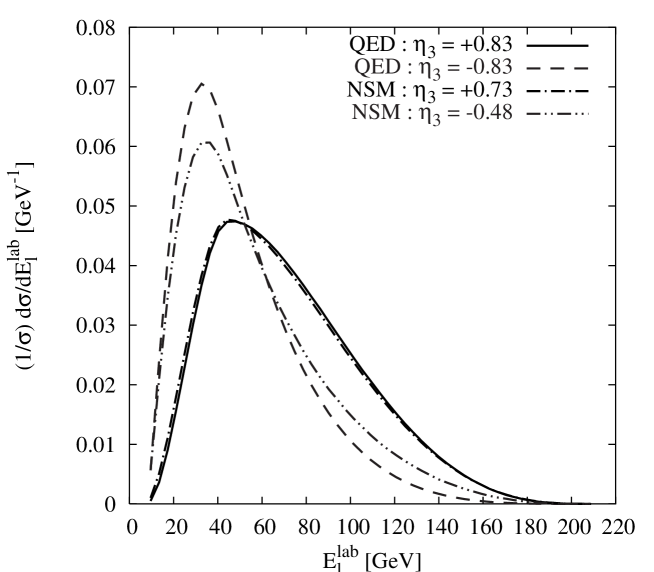
For simplicity, we consider a massless $b$ quark and a narrow-width approximation for the $W$ boson. With the former assumption only $f_{2R}$ contributes to the $E_{\ell}$ distribution. We consider the production process $\gamma\gamma\to t\bar{t}$ with/without contribution from $\gamma\gamma\to\phi\to t\bar{t}$ [4], where $\phi$ is a non-standard model (NSM) Higgs boson of mass 475 GeV, width 2.5 GeV. Further, we take for the top couplings ($S_{t}$, $P_{t}$) and the $\gamma$ couplings ($S_{\gamma}$, $P_{\gamma}$) of the Higgs boson, defined in Ref. [4], the following arbitrarily chosen values : $S_{t}=0.2,\ P_{t}=0.4,\ S_{\gamma}=4.0+i\ 0.5\ \mbox{and}\ P_{\gamma}=1.25+i\ 2.0.$ We then study the change in polarization of the $t$ quark and its effect on the $E_{\ell}$ distribution. We use the ideal photon spectrum of [55] and calculate various kinematical distributions for initial-state polarizations

$$P^{+}\ \equiv\ \lambda_{e^{-}}=\lambda_{e^{+}}=+,\ \lambda_{1}=\lambda_{2}=-\hskip 14.22636pt\mbox{and}\hskip 14.22636ptP^{-}\ \equiv\ \lambda_{e^{-}}=\lambda_{e^{+}}=-,\ \lambda_{1}=\lambda_{2}=+.$$

For a PLC running at 600 GeV, the QED prediction for polarization is $+0.83$ with a $P^{+}$ initial state and $-0.83$ with a $P^{-}$ initial state. The polarization in the presence of a non-standard Higgs boson is $+0.73$ and $-0.48$ for $P^{+}$ and $P^{-}$ initial states respectively. For the two choices of polarized initial states the $E_{\ell}$ distribution is shown in Fig. 3 for both QED and (NSM Higgs + QED), where the latter is denoted by “NSM”. Here $f_{2R}=0$ is assumed. We see that the $E_{\ell}$ distribution is peaked at lower values of $E_{\ell}$ when the $t$ quark is negatively polarized and the peak of the distribution is shifted to a higher value for positively polarized $t$ quarks. This can be understood as follows. In the rest frame of the $t$ quark the angular distribution of leptons is $(1+\eta_{3}\cos\theta_{\ell})$. Thus for a positively polarized $t$ quark most of the decay leptons come in the forward direction, i.e. the direction of the would-be momentum of the $t$ quark. Thus a boost from the rest frame to the lab frame increases the energies of these leptons. This explains the shifted position of the peak for a positively polarized $t$ quark. Similarly, for negative polarization most of the decay leptons come out in the backward direction w.r.t. the lab momentum of the $t$ quark. This results in an opposite boost and hence a decrease in the energy of the leptons. In other words, it leads to increase in lepton counts for lower energy. This explains the large peak in $E_{\ell}$ distribution at lower $E_{\ell}$. Further, for the case of $P^{-}$ initial state, there are large modifications in the values of $t$ polarization due to the Higgs contribution as compared to the pure QED prediction. These large differences show up in the dashed and dashed-double-dotted curves in Fig. 3.

Figure 4: The distribution in the energy of the lepton in the lab frame within QED for different values of $\Re(f_{2R})$, with $P^{+}$ (left panel) and $P^{-}$ (right panel) initial states.

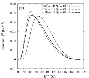
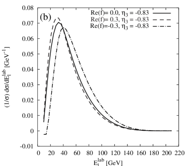
The $E_{\ell}$ distribution is obviously dependent on the anomalous $tbW$ couplings and the dependence is shown in Fig. 4 for different values of $f(=f_{2R})$ and initial states $P^{+}$ and $P^{-}$. Thus we see that the $E_{l}$ distribution in the lab frame is affected by the polarization of the decaying $t$ quarks as well as by the anomalous $tbW$ couplings. Thus $E_{\ell}$ distribution cannot be used as a definite signal for either $t$ polarization or anomalous $tbW$ couplings in the lab frame due to their intermingled effects.

Figure 5: The distribution in the energy of the lepton in the rest frame within QED for different values of $\Re(f_{2R})$ with $P^{+}$ initial state.

In the rest frame of the $t$ quark, however, the angular and energy dependences are decoupled from each other. Hence the energy distribution is independent of the $t$ polarization which in turn may depend on the production process. The $E_{\ell}^{0}$ distribution is given by

$$\frac{1}{\sigma}\ \frac{d\sigma}{dE_{\ell}^{0}}=\frac{1}{\Gamma_{t}(\ell)}\ \left(\frac{\alpha^{2}}{8\ \sin^{4}\theta_{W}}\right)\ \frac{1}{\pi\ m_{t}}\ E_{\ell}^{0}F(E_{\ell}^{0})\ \left|\Delta_{W}(p_{W}^{2})\right|^{2}\ dp_{W}^{2},$$ (32)

independent of the production process. Here $\Gamma_{t}(\ell)$ is the partial decay width of the $t$ quark in the semi-leptonic channel. We note that $\Gamma_{t}(\ell)$ depends upon anomalous $tbW$ couplings. For massless $b$ quarks and on-shell $W$ bosons the $E_{\ell}$ distribution reduces to

$$\frac{1}{\sigma}\ \frac{d\sigma}{dE_{\ell}^{0}}=\frac{1}{\Gamma_{t}(\ell)}\ \left(\frac{\alpha^{2}}{8\ \sin^{4}\theta_{W}}\right)\ \frac{1}{m_{t}\ m_{W}\ \Gamma_{W}}\ E_{\ell}^{0}\ (m_{t}^{2}-2m_{t}\ E_{\ell}^{0})\ \left(1+\Re(f_{2R})\ \frac{m_{W}}{E_{\ell}^{0}}\right),$$ (33)

while the semi-leptonic partial decay width is given by

$$\Gamma_{t}(\ell)=\left(\frac{\alpha^{2}}{192\ \sin^{4}\theta_{W}}\right)\ \frac{1}{m_{t}m_{W}\Gamma_{W}}\ \frac{(m_{t}^{2}-m_{W}^{2})^{2}}{m_{t}^{2}}\ \left(m_{t}^{2}+2m_{W}^{2}+6\ \Re(f_{2R})\ m_{t}m_{W}\right).$$

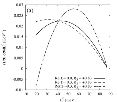
Thus we see that the energy distribution of the decay lepton is completely independent of the production process, the kinematical distribution of the $t$ quark or its polarization. It depends only on $\Re(f_{2R})$ and is shown in Fig. 5. The distribution shows a strong dependence on $\Re(f_{2R})$. The crossing point in the distribution is at $E_{\ell}^{C}=(m_{t}+2m_{W}^{2}/m_{t})/6=41.5$ GeV when there is an accidental cancellation between $\Re(f_{2R})$-dependent terms in $F(E_{\ell})$ and $\Gamma_{t}(\ell)$. One can define an asymmetry about this crossing point as

$$A_{E_{\ell}}=\frac{\sigma(E_{\ell}^{0}>E_{\ell}^{C})-\sigma(E_{\ell}^{0}<E_{\ell}^{C})}{\sigma(E_{\ell}^{0}>E_{\ell}^{C})+\sigma(E_{\ell}^{0}<E_{\ell}^{C})}\ =\ \frac{13m_{t}^{2}-22m_{W}^{2}-18\Re(f_{2R})\ m_{t}m_{W}}{27\ (m_{t}^{2}+2m_{W}^{2}+6\Re(f_{2R})\ m_{t}m_{W})}.$$ (34)

This asymmetry is sensitive to $\Re(f_{2R})$, the anomalous $tbW$ coupling. If the four-momentum of the decaying $t$ quark is fully reconstructed the rest-frame lepton energy can be computed as $E_{\ell}^{0}=(p_{t}\cdot p_{\ell})/m_{t}$ and the distribution shown in Fig. 5 can be generated. Then using the asymmetry $A_{E_{\ell}}$ the value of $\Re(f_{2R})$ can be measured independent of any possible new physics in the production process. This is another manifestation of the decoupling of the lepton angular distribution.

Thus, if $p_{t}$ can be fully reconstructed then the spin-basis vectors $s_{i}$ can be constructed. Using Eq. (30) one can then probe the polarization of the $t$ quark and any new physics in the production process, independent of anomalous $tbW$ couplings using the angular distribution of the decay leptons. At the same time, using the $E_{\ell}^{0}(=(p_{t}\cdot p_{\ell})/m_{t})$ distribution and $A_{E_{\ell}}(f)$, one can probe anomalous $tbW$ couplings independent of the new physics in the production process of the $t$ quark. It is interesting to note that the scalar product of $p_{\ell}$ with $p_{t}$ and $s_{i}$can probe effects of new physics in both production and decay processes of $t$ quarks. The quantity $(p_{t}\cdot p_{\ell})$ is sensitive only to the new physics in the decay vertex independent of the production process or dynamics, while $(s_{i}\cdot p_{\ell})$ are sensitive only to the production dynamics independent of anomalous contributions to the top decay vertex.

6 Simple and qualitative probes of $t$ polarization

A completely decoupled analysis of possible new physics in production and decay processes of the $t$ quark is possible. However, such an analysis necessarily requires full reconstruction of the four-momentum of the $t$ quark. Full reconstruction of $p_{t}$ is not always possible and it is useful to to look for some easily measurable variables or distributions, which could probe $t$ polarization. The lab frame distribution of the lepton energy shows sensitivity to the $t$ polarization, but it is contaminated by possible presence of anomalous $tbW$ couplings. The lab frame lepton angular distribution, on the other hand, is insensitive to the anomalous $tbW$ couplings and can be used at least as a qualitative probe of $t$ polarization. For demonstration purposes we again consider top-pair production at a PLC as in the last section.

Figure 6: The distributions in the cosines of the angles of the top and the lepton, $\cos\theta_{t}$ and $\cos\theta_{\ell}$, respectively, in the lab frame with $P^{+}$ (left panel) and $P^{-}$ (right panel) initial states. For pure QED we have $\eta_{3}=\pm 0.83$ while the presence of a Higgs boson modifies it to $+0.73$ and $-0.48$ for $P^{+}$ and $P^{-}$ initial states, respectively.

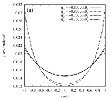
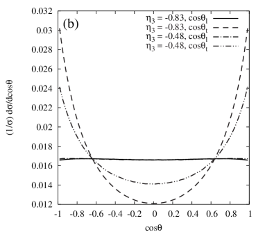
The $\cos\theta_{\ell}$ and $\cos\theta_{t}$ distributions with $P^{+}$ and $P^{-}$ states are shown in Fig. 6. In Fig. 6(a), which is drawn for the $P^{+}$ initial state, we see that the lepton distribution follows the distribution of the $t$ quark in the lab frame up to some kinematical smearing. On the other hand, for the $P^{-}$ initial state, the lepton distribution is flat, i.e., it is completely smeared out. This is the effect of the polarization of the $t$ quark, which is different in the two cases. For the pure QED case, the distribution of the $t$ quark is exactly the same (the dashed line in both Fig. 6(a) and (b)), while the polarization is $+0.83$ in the first case and $-0.83$ in the second. Since positively polarized $t$ quarks have leptons focused in the forward direction and negatively polarized $t$ quarks in the backward direction, the corresponding lepton distribution (solid line) is quite different for the two cases in the lab frame. Any change in the $t$-quark angular distribution, such as caused by the NSM Higgs boson (dashed-double-dotted line), can also change the lepton polar distribution. Secondly, one needs to know the $\cos\theta_{t}$ distribution, i.e., the production process, before hand in order to estimate its polarization based on $\cos\theta_{\ell}$ distribution. Thus the lepton polar distribution in the lab frame captures the effect of $t$ polarization only in a qualitative way as in the case of the $E_{\ell}$ distribution. One advantage that the $\cos\theta_{\ell}$ distribution has is that it is insensitive to anomalous $tbW$ couplings and depends only upon the dynamics of the production process.

Figure 7: The distribution in the azimuthal angle of the lepton, as defined in the text, in the lab frame with $P^{+}$ and $P^{-}$ initial states for $t$ quarks with different polarizations.

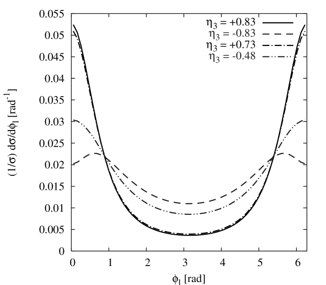
The azimuthal distribution of the secondary leptons w.r.t. the production plane of the $t$ quark also captures the effect of $t$ polarization in a qualitative way. The skewness of the azimuthal distribution is related to $\eta_{2}$, the net transverse polarization of the decaying $t$ quark perpendicular to the production plane. $\eta_{1}$ and $\eta_{3}$ are degrees of polarization in the production plane and lead to symmetric distribution about the production plane. In the present case of $t\bar{t}$ production at a PLC through a Higgs boson, the net transverse polarization is zero, i.e., $\eta_{1}=\eta_{2}=0$. Thus, the $\phi_{\ell}$ distribution is symmetric about the $t$-production plane and shows sensitivity to $\eta_{3}$, the longitudinal polarization, as shown in Fig. 7. We see that for a positively polarized $t$ quark the $\phi_{\ell}$ distribution is peaked near $\phi_{\ell}=0(2\pi)$ and the height of the peak decreases as the polarization changes from $+0.83$ to $-0.83$. This again is related to the $(1+\eta_{3}\cos\theta_{\ell})$ distribution of the decay lepton in the rest frame of the $t$ quark, which upon boosting experiences relativistic focusing and leads to a larger peak for positive polarization and a smaller peak or suppression for negative polarization. Unlike $E_{\ell}$ or $\cos\theta_{\ell}$ distributions, the $\phi_{\ell}$ distribution can be used to quantify the $t$ polarization. The up-down asymmetry is related to $\eta_{2}$ as shown in Eq. (30). The peak height and the fractional area of the distribution near the peak are qualitative measures of “in-plane” polarization of $t$ quarks.

Thus, in conclusion, the angular distribution of decay leptons itself provides a qualitative probe of the $t$ polarization in the lab frame of the $\gamma\gamma$ collider. Similar trends are expected for other colliders such as the LHC and LC and also for a general $2\to n$ process of $t$-quark production.

7 The $b$-quark angular distribution

Even though the lepton angular and energy distributions offer a rather neat way of probing $t$ polarization, this probe suffers from the rather low leptonic branching ratio of the $W$ and the consequent small number of events that can be used for the purpose. Indeed, this situation may be improved upon by using the $b$-quark angular distribution. In this section we outline how this may be done.

We consider a generic process of $t$-quark production followed by $t\to bW$. The full differential cross-section is given by

$$d\sigma = \sum_{\lambda,\lambda^{\prime}}\left[\frac{(2\pi)^{4}}{2I}\rho(\lambda,\lambda^{\prime})\delta^{4}\bigg{(}k_{A}+k_{B}-p_{t}-\bigg{(}\sum_{i}^{n-1}p_{i}\bigg{)}\bigg{)}\frac{d^{3}p_{t}}{2E_{t}(2\pi)^{3}}\ \prod_{i}^{n-1}\frac{d^{3}p_{i}}{2E_{i}(2\pi)^{3}}\right]$$ (35)

$$\times \left(\frac{1}{\Gamma_{t}}\right)\ \left[\frac{(2\pi)^{4}}{2m_{t}}\Gamma(\lambda,\lambda^{\prime})\delta^{4}(p_{t}-p_{b}-p_{\nu}-p_{\ell})\frac{d^{3}p_{b}}{2E_{b}(2\pi)^{3}}\ \frac{d^{3}p_{W}}{2E_{W}(2\pi)^{3}}\right],$$

for a narrow $t$ quark, similar to Eq. (16). The above equation assumes an on-shell $W$ boson. The expression for the decay density matrix for $t\to bW$, assuming a massless $b$ quark, is obtained as

$$\Gamma(\pm,\pm) = \frac{g^{2}\ m_{t}^{2}}{2}\left[{\cal C}_{1}\pm{\cal C}_{2}\ \cos\theta_{b}\right]$$

$$\Gamma(\pm,\mp) = \frac{g^{2}\ m_{t}^{2}}{2}\ \left[{\cal C}_{2}\ \sin\theta_{b}\ e^{\pm\phi_{b}}\right],$$ (36)

where

$${\cal C}_{1} = \left(\frac{1}{2}+\frac{m_{t}^{2}}{2\ m_{W}^{2}}-\frac{m_{W}^{2}}{m_{t}^{2}}\right)+3\Re(f_{2R})\left(\frac{m_{t}}{m_{W}}-\frac{m_{W}}{m_{t}}\right),$$

$${\cal C}_{2} = \left(\frac{3}{2}-\frac{m_{t}^{2}}{2\ m_{W}^{2}}-\frac{m_{W}^{2}}{m_{t}^{2}}\right)+\Re(f_{2R})\left(\frac{m_{t}}{m_{W}}-\frac{m_{W}}{m_{t}}\right).$$ (37)

Thus, in the rest frame of the decaying the $t$ quark, the angular distribution of the $b$ quark, similar to Eq. (27), is given by

$$\frac{d\sigma}{d\cos\theta_{b}\ d\phi_{b}}=\frac{\sigma_{tot}}{4\pi}\ \left[1+\frac{{\cal C}_{2}}{{\cal C}_{1}}\ \left(\eta_{3}\ \cos\theta_{b}+\eta_{1}\ \sin\theta_{b}\cos\phi_{b}+\eta_{2}\ \sin\theta_{b}\sin\phi_{b}\right)\right].$$ (38)

Hence the expressions for the $t$ polarization, similar to Eq.(30), can be written as

$$\frac{\eta_{3}}{2}\ \frac{{\cal C}_{2}}{{\cal C}_{1}} = \frac{\sigma(p_{b}.s_{3}<0)-\sigma(p_{b}.s_{3}>0)}{\sigma_{tot}}$$

$$\frac{\eta_{2}}{2}\frac{{\cal C}_{2}}{{\cal C}_{1}} = \frac{\sigma(p_{b}.s_{2}<0)-\sigma(p_{b}.s_{2}>0)}{\sigma_{tot}}$$

$$\frac{\eta_{1}}{2}\frac{{\cal C}_{2}}{{\cal C}_{1}} = \frac{\sigma(p_{b}.s_{1}<0)-\sigma(p_{b}.s_{1}>0)}{\sigma_{tot}}.$$ (39)

Thus, for $b$-quark distributions the anomalous $tbW$ couplings enters through factors ${\cal C}_{1}$ and ${\cal C}_{2}$, or rather, through their ratio which is given by

$$\frac{{\cal C}_{2}}{{\cal C}_{1}} = -\left(\frac{m_{t}^{2}-2\ m_{W}^{2}}{m_{t}^{2}+2\ m_{W}^{2}}\right)+\Re(f_{2R})\ \left(\frac{8\ m_{t}m_{w}(m_{t}^{2}-m_{W}^{2})}{(m_{t}^{2}+2m_{W}^{2})^{2}}\right)$$ (40)

$$\equiv \alpha_{b}^{0}+\Re(f_{2R})\ \alpha_{b}^{1}.$$

Here we have retained terms only up to linear order in $f_{2R}$. For $m_{t}=175$ GeV and $m_{W}=80.41$ GeV we have

$$\alpha_{b}^{0}=-0.406,\hskip 28.45274pt\alpha_{b}^{1}=1.43\ .$$

In other words, the sensitivity of the $b$-quark distribution to the $t$ polarization is less than that of the lepton distribution, the analyzing powers being in the ratio $[-0.406+1.43\ \Re(f_{2R})~{}:~{}1.00]$. Thus the gain due to the larger statistics is offset by the low sensitivity, and overall there is not much gain. However if we consider $b$-quark angular asymmetries, Eq. (39), in association with the corresponding lepton angular asymmetries, Eq. (30), we have

$${\rm Br}(t\to b\ell\nu_{\ell})\frac{\left[\sigma(p_{b}.s_{i}<0)-\sigma(p_{b}.s_{i}>0)\right]}{\sigma(p_{\ell}.s_{i}<0)-\sigma(p_{\ell}.s_{i}>0)}=\frac{{\cal C}_{2}}{{\cal C}_{1}}=\alpha_{b}^{0}+\Re(f_{2R})\ \alpha_{b}^{1}.$$ (41)

The ratio of the $b$-quark asymmetry to the leptonic asymmetry depends on the anomalous $tbW$ coupling linearly and can be used to measure $\Re(f_{2R})$. However, such a measurement is possible only if the $t$ polarization is large. Considering only the semi-leptonic decay channel of the $t$ quark, the expected limit on $\Re(f_{2R})$ is given by

$$|\Re(f_{2R})|\leq\frac{f}{|\eta_{i}|\ \sqrt{{\cal L}\ \sigma}}\frac{\sqrt{1+(\alpha_{b}^{0})^{2}}}{\alpha_{b}^{1}}\ .$$ (42)

Here, ${\cal L}$ is the integrated luminosity, $\sigma$ is the total rate of $t$-quark production and its semi-leptonic decay, $f$ is the degree of statistical significance and $\eta_{i}$ is the average polarization of the decaying $t$ quark. We note that the limit in Eq.(42) is independent of the production mechanism of the $t$ quark but depends upon the average polarization of the $t$ quark. The $t$-quark pair-production rate at an $e^{+}e^{-}$ collider is large and for polarized electron and positron beams the $t$ quark is highly polarized. Hence it is the best and the cleanest place to measure $\Re(f_{2R})$. Alternatively, one can undertake measurements at LHC where the $t\bar{t}$ production rate is very high $\sim 750$ pb. QCD corrections may lead to $\eta_{2}\approx 10^{-3}$ in $q\bar{q}$ fusion [21] while possible new physics in the production process may give a larger value of $\eta_{2}$. Further, the measurement of $\eta_{2}$ requires re-construction of only the production plane of the $t$ quark, which is possible at LHC. Thus one sees from Eq.(42) that for $i=2$, using the asymmetry of Eq.(41) and assuming $|\eta_{2}|=0.01$, one may be able to constrain $\Re(f_{2R})$ within $0.05$ at 95% C.L. with about $8\times 10^{7}$ events for top quark. We emphasize that this estimate of number of events does not assume anything about mechanism or kinematics of $t$ quark production. For this analysis one has to look only at the semi-leptonic decay channel of the $t$ quarks as that has rather small radiative corrections.

8 Discussions and Conclusions

The decoupling of decay-lepton angular distribution from anomalous couplings in the $tbW$ vertex has been known for $e^{+}e^{-}\to t\bar{t}$ [1, 2], $\gamma\gamma\to t\bar{t}$ [3, 4] and also for a general $2\to 2$ [5, 6] process of $t$-quark pair production. All these results have used the narrow-width approximation for $W$ bosons and except for Ref. [6] all of them assume a massless $b$ quark. The vanishing mass of the $b$ quark provides additional chiral symmetry and among the anomalous couplings shown in Eq. (1) only $f_{2R}$ contributes. In the present work we extended this decoupling theorem to a general $2\to n$ process of $t$-quark production with a massive $b$ quark (hence keeping all four anomalous $tbW$ couplings) and without using the narrow-width approximation for $W$ bosons. We analyzed the essential inputs for the decoupling and found that the narrow-width approximation for $t$ quarks and smallness of $\{f_{1R},\ f_{2L},\ f_{2R}\}$ are the only two requisites for decoupling. This decoupling can also be extended to the hadronic decay of $W$ bosons where the role of $\ell$ is taken up by the down-type quark, i.e. $T_{3}=-1/2$ fermion in the $SU(2)$ doublet. The charge measurement of the light-quark jets is the only technical barrier in using this channel. We argue that within the narrow-width approximation, the decoupling of the lepton angular distribution remains valid after radiative corrections, while noting that the decoupling of the angular distribution of the down-type quark receives about 7% correction from QCD contributions.

The polarization of the $t$ quark reflects in the kinematic distribution of its decay products. We use the decoupled lepton angular distribution to construct specific asymmetries (Eq. (30)) to measure the $t$ polarization. These asymmetries, robust against radiative corrections since they are constructed after taking ratios, are insensitive to the anomalous $tbW$ coupling. A full reconstruction of the four-momentum of the $t$ quark is necessary to construct these asymmetries experimentally, which may be possible only at the ILC. At the LHC or the PLC one can construct the $t$-production plane and hence $\eta_{2}$ can be constructed, which is sensitive to the absorptive part of the production amplitude. The energy distribution of the decay lepton shows sensitivity to new physics in the decay process, i.e. the $tbW$ vertex. In the lab frame it receives contribution both from the polarization of the $t$ quark and possible anomalous $tbW$ couplings. However, in the rest frame of the $t$ quark it is sensitive only to the anomalous $tbW$ couplings and is independent of the type of production process as well as any possible new physics in the production process. Thus given full reconstruction of the $t$ quark four-momentum, possible new physics in production and decay processes of the $t$ quark can be studied independent of each other using angular and energy distributions of secondary leptons, respectively.

We also studied the effect of $t$ polarization on the lepton angular distribution in the lab frame. Such an analysis is useful where momentum reconstruction is not possible. We see that the $\cos\theta_{\ell}$ and $\phi_{\ell}$ distributions in the lab frame of a $\gamma\gamma$ collider are sensitive to the polarization of the decaying top, at least in a qualitative way. A quantitative estimate is possible for $\eta_{2}$, which can be obtained using the up-down asymmetry of decay leptons w.r.t. the $t$-production plane.

To summarize, we have demonstrated that the lepton distribution can be used to probe new physics contributions in the production and the decay processes of the $t$ quark, separately, independent of each other. The lepton angular distribution is shown to be completely insensitive to any anomalous $tbW$ coupling assuming the $t$ quark to be on-shell and anomalous $tbW$ couplings to be small. The energy distribution in the rest frame of the $t$ quark, on the other hand, was found to be sensitive only to the anomalous $tbW$ couplings. We construct specific asymmetries involving the lepton angular distribution w.r.t. the top momentum, to measure its polarization in a generic process of $t$-quark production. The qualitative features of the lab-frame angular distribution of the decay leptons have been shown to be sensitive to the polarization of the decaying $t$ quark.

Acknowledgments
This work was partially supported by Department of Science and Technology project SP/S2/K-01/2000-II and Indo French Centre for Promotion of Advanced Research Project 3004-2. We also thank the funding agency Board for Research in Nuclear Sciences and the organizers of the 8th Workshop on High Energy Physics Phenomenology (WHEPP8), held at the Indian Institute of Technology, Mumbai, January 5-16, 2004, where this work was initiated.

Appendix A Momentum reconstruction for the $t$ quark

In a generic reaction of $t$-quark production and subsequent decay of unstable particles, (partial) reconstruction of $p_{t}$ is possible if there is only one or no missing neutrino in the final debris. For the semi-leptonic decay of $t$ quarks there is one neutrino, thus we demand that all other particles in the production part are observable or decay into observable particles. The cases of different colliders are discussed.

Fixed $\sqrt{s}$ collider : The $e^{+}e^{-}$ linear collider is an example of a fixed $\sqrt{s}$ collider. At these colliders the net three-momentum of the various particles should add up to zero. Since we have only one neutrino, its three-momentum can be determined and hence $p_{t}$ can be fully reconstructed. Thus the study of polarization of the $t$ quark at an $e^{+}e^{-}$ collider is possible through the analysis of the decay-lepton angular distributions.

Variable $\sqrt{s}$ colliders : Hadron colliders and photon colliders are variable $\sqrt{s}$ colliders. The c.m. frame of colliding partons moves with an unknown momentum along the beam axis of the collider. Thus the three-momenta of the final state particles should add up to $\vec{P}_{cm}$ which is parallel to the $z$ axis. This implies that the transverse momentum of all particles should add up to zero. This immediately gives the transverse momentum of neutrino and hence transverse momentum of the $t$ quark. This defines the production plane of the $t$ quark and one can construct $\eta_{2}$, the transverse polarization of the $t$ quark normal to the production plane. Since construction of $\eta_{2}$ is possible at LHC and since the top is produced through QCD interaction at LHC, one can study the absorptive part of the QCD corrections to the production process via lepton distributions.

References

- [1] S. D. Rindani, Pramana 54, 791 (2000)
- [2] B. Grzadkowski and Z. Hioki, Phys. Lett. B 476, 87 (2000); Z. Hioki, hep-ph/0104105.
- [3] K. Ohkuma, Nucl. Phys. B (Proc. Suppl.) 111, 285 (2002);
- [4] R. M. Godbole, S. D. Rindani and R. K. Singh, Phys. Rev. D 67, 095009 (2003) [Erratum-ibid. D 71, 039902 (2005)]
- [5] B. Grzadkowski and Z. Hioki, Phys. Lett. B 529, 82 (2002).
- [6] B. Grzadkowski and Z. Hioki, Phys. Lett. B 557, 55 (2003); Z. Hioki, hep-ph/0210224.
- [7] R. H. Dalitz and G. R. Goldstein, Phys. Rev. D 45, 1531 (1992);
- [8] T. Arens and L. M. Sehgal, Nucl. Phys. B 393, 46 (1993).
- [9] B. Grzadkowski, B. Lampe and K. J. Abraham, Phys. Lett. B 415, 193 (1997) [arXiv:hep-ph/9706489].
- [10] D. Espriu and J. Manzano, Phys. Rev. D 66, 114009 (2002);
- [11] E. Christova and D. Draganov, Phys. Lett. B 434, 373 (1998).
- [12] B. Grzadkowski, Phys. Lett. B 305, 384 (1993) [arXiv:hep-ph/9303204].
- [13] M. Fischer S. Groote, J. G. Körner, M. C. Mauser and B. Lampe, Phys. Lett. B 451, 406 (1999).
- [14] C. A. Nelson, E. G. Barbagiovanni, J. J. Berger, E. K. Pueschel and J. R. Wickman, Eur. Phys. J. C 45, 121 (2006) [arXiv:hep-ph/0506240]; C. A. Nelson, J. J. Berger and J. R. Wickman, Eur. Phys. J. C 46, 385 (2006) [arXiv:hep-ph/0510348].
- [15] S. Tsuno, I. Nakano, Y. Sumino and R. Tanaka, Phys. Rev. D 73, 054011 (2006) [arXiv:hep-ex/0512037].
- [16] Y. Sumino and S. Tsuno, Phys. Lett. B 633, 715 (2006) [arXiv:hep-ph/0512205].
- [17] O. Terazawa, Int. J. Mod. Phys. A 10, 1953 (1995).
- [18] S. Atag and B. D. Sahin, arXiv:hep-ph/0404283.
- [19] C. P. Yuan, Phys. Rev. D 45, 782 (1992).
- [20] G. A. Ladinsky, Phys. Rev. D 46, 3789 (1992) [Erratum-ibid. D 47, 3086 (1993)].
- [21] W. Bernreuther, A. Brandenburg and P. Uwer, Phys. Lett. B 368, 153 (1996)
- [22] Y. Akatsu and O. Terazawa, Int. J. Mod. Phys. A 12, 2613 (1997).
- [23] W. Bernreuther, J. P. Ma and T. Schroder, Phys. Lett. B 297, 318 (1992).
- [24] G. L. Kane, G. A. Ladinsky and C. P. Yuan, Phys. Rev. D 45, 124 (1992).
- [25] R. Harlander, M. Jezabek, J. H. Kuhn and T. Teubner, Phys. Lett. B 346, 137 (1995)
- [26] M. Jezabek, Nucl. Phys. Proc. Suppl. 51C (1996) 60.
- [27] R. Harlander, M. Jezabek, J. H. Kuhn and M. Peter, Z. Phys. C 73, 477 (1997)
- [28] B. M. Chibisov and M. B. Voloshin, Mod. Phys. Lett. A 13, 973 (1998)
- [29] M. Awramik and M. Jezabek, Acta Phys. Polon. B 32, 2115 (2001)
- [30] Q. J. Zhang, C. S. Li, J. J. Liu and L. G. Jin, Commun. Theor. Phys. 40, 687 (2003) [arXiv:hep-ph/0303228].
- [31] S. J. Parke and Y. Shadmi, Phys. Lett. B 387, 199 (1996) [arXiv:hep-ph/9606419].
- [32] A. Brandenburg, Phys. Lett. B 388, 626 (1996) [arXiv:hep-ph/9603333].
- [33] G. Mahlon and S. J. Parke, Phys. Lett. B 411, 173 (1997) [arXiv:hep-ph/9706304].
- [34] M. Hori, Y. Kiyo and T. Nasuno, Phys. Rev. D 58, 014005 (1998) [arXiv:hep-ph/9712379].
- [35] A. Brandenburg and Z. G. Si, Phys. Lett. B 615, 68 (2005) [arXiv:hep-ph/0503153].
- [36] M. M. Tung, J. Bernabeu and J. Penarrocha, Phys. Lett. B 418, 181 (1998) [arXiv:hep-ph/9706444].
- [37] A. Brandenburg, M. Flesch and P. Uwer, Phys. Rev. D 59, 014001 (1999) [arXiv:hep-ph/9806306].
- [38] J. Kodaira, T. Nasuno and S. J. Parke, Phys. Rev. D 59, 014023 (1999) [arXiv:hep-ph/9807209].
- [39] W. Bernreuther, A. Brandenburg and Z. G. Si, Phys. Lett. B 483, 99 (2000) [arXiv:hep-ph/0004184].
- [40] Y. Kiyo, J. Kodaira and K. Morii, Eur. Phys. J. C 18, 327 (2000) [arXiv:hep-ph/0008065].
- [41] Y. Kiyo, J. Kodaira, K. Morii, T. Nasuno and S. J. Parke, Nucl. Phys. Proc. Suppl. 89, 37 (2000) [arXiv:hep-ph/0006021].
- [42] W. Bernreuther, A. Brandenburg, Z. G. Si and P. Uwer, Phys. Rev. Lett. 87, 242002 (2001) [arXiv:hep-ph/0107086].
- [43] W. Bernreuther, A. Brandenburg, Z. G. Si and P. Uwer, Phys. Lett. B 509, 53 (2001) [arXiv:hep-ph/0104096].
- [44] J. A. Aguilar-Saavedra, J. Carvalho, N. Castro and A. Onofre, arXiv:hep-ph/0605190.
- [45] M. M. Najafabadi, arXiv:hep-ph/0601155.
- [46] P. Poulose and S. D. Rindani, Phys. Lett. B 349, 379 (1995) [arXiv:hep-ph/9410357]; Phys. Rev. D 54, 4326 (1996) [Erratum-ibid. D 61, 119901 (2000)] [arXiv:hep-ph/9509299]; Phys. Lett. B 383, 212 (1996) [arXiv:hep-ph/9606356]; S. D. Rindani, Pramana 61, 33 (2003) [arXiv:hep-ph/0304046].
- [47] P. Poulose and S. D. Rindani, Phys. Rev. D 57, 5444 (1998) [Erratum-ibid. D 61, 119902 (2000)] [arXiv:hep-ph/9709225]; Phys. Lett. B 452, 347 (1999) [arXiv:hep-ph/9809203].
- [48] M. Jezabek and J. H. Kuhn, Nucl. Phys. B 320, 20 (1989). A. Czarnecki, M. Jezabek and J. H. Kuhn, Nucl. Phys. B 351, 70 (1991).
- [49] A. Brandenburg, Z. G. Si and P. Uwer, Phys. Lett. B 539, 235 (2002) [arXiv:hep-ph/0205023].
- [50] W. Beenakker, F. A. Berends and A. P. Chapovsky, Phys. Lett. B 454, 129 (1999) [arXiv:hep-ph/9902304].
- [51] C. Macesanu, Phys. Rev. D 65, 074036 (2002) [arXiv:hep-ph/0112142].
- [52] K. Kolodziej, A. Staron, A. Lorca and T. Riemann, Eur. Phys. J. C 46, 357 (2006) [arXiv:hep-ph/0510195].
- [53] K. Melnikov and O. I. Yakovlev, Phys. Lett. B 324, 217 (1994).
- [54] W. Bernreuther, A. Brandenburg, Z. G. Si and P. Uwer, Nucl. Phys. B 690, 81 (2004) [arXiv:hep-ph/0403035].
- [55] I. F. Ginzburg, G. L. Kotkin, S. L. Panfil, V. G. Serbo and V. I. Telnov, Nucl. Instrum. Meth. 219, 5 (1984).