Phase space and quark mass effects in neutrino emissions in a color superconductor

Abstract

We study the phase space for neutrino emissions with massive quarks in direct Urca processes in normal and color superconducting quark matter. We derive in QCD and the NJL model the Fermi momentum reduction resulting from Fermi liquid properties which opens up the phase space for neutrino emissions. The relation between the Fermi momentum and chemical potential is found to be $p_{F}\approx\mu(1-\kappa)$ with $\kappa$ depending on coupling constants. We find in the weak coupling regime that $\kappa$ is a monotonously increasing function of the chemical potential. This implies quenched phase space for neutrino emissions at low baryon densities. We calculate neutrino emissivities with massive quarks in a spin-one color superconductor. The quark mass corrections are found to be of the same order as the contributions in the massless case, which will bring sizable effects on the cooling behavior of compact stars.

I Introduction and Conclusion

The baryon density in the core of a compact star is likely to reach several times the nuclear saturation density, $\rho_{0}\sim 0.16\;\mathrm{fm}^{-3}$ or $2.7\times 10^{14}\mathrm{g}/\mathrm{cm}^{3}$. At such a high density, nucleons in nuclear matter are crushed into their constituents, i.e. quarks and gluons. Itoh proposed a model for quark stars in 1970 Itoh:1970uw . The deconfinement transition to quark matter was suggested by Collins and Perry in 1975 Collins:1974ky based on the asymptotic freedom in quantum chromodynamics. In the same paper they also mentioned the possibility that quark matter could be a superfluid or a superconductor resulting from the attractive interquark force in some channels. Barrois, Bailin and Love developed this novel idea and studied the unusual variant of superconductivity in quark matter, which we now call color superconductivity Barrois:1977xd ; Bailin:1983bm . They did their calculations in the framework of weak coupling approach and did not take into account the dynamic screening of magnetic gluons which are dominant agents in pairing quarks. Therefore the gap or equivalently the transition temperature they obtained are too small to be of relevance to any sizable observables. About fifteen years later the color superconductivity had been re-discovered by several groups who found the gap could be large enough to bring some real effects in compact stars Alford:1997zt ; Alford:1998mk ; Rapp:1997zu ; Son:1998uk ; Pisarski:1999tv ; Hong:1999fh . [For recent reviews on color superconductivity, see, for example, Rajagopal:2000wf ; Alford:2001dt ; Reddy:2002ri ; Casalbuoni:2003wh ; Schafer:2003vz ; Rischke:2003mt ; Buballa:2003qv ; Ren:2004nn ; Shovkovy:2004me .]

At asymptotically high baryon density or chemical potential, the color-flavor locked (CFL) phase is favored Alford:1998mk . The rigorous weak coupling approach of QCD Son:1998uk ; Pisarski:1999tv ; Brown:1999aq ; Wang:2001aq ; Schmitt:2002sc ; Ipp:2003cj ; Reuter:2004kk ; Gerhold:2005uu ; Noronha:2006cz is justified. [For recent reviews on the QCD weak coupling approach in normal dense quark matter or in color superconductivity, see Rischke:2003mt ; Ren:2004nn ; Wang:2004pa ; Rebhan:2005hw ; Gerhold:2005fi ; Gerhold:2005nt ; Reuter:2006iw .] The situation is more complicated at lower densities realized in compact stars. In this case, the strange quark mass $m_{s}$ is in the range from its current mass $\sim$100 MeV to its constituent mass $\sim$500 MeV. The main effect of $m_{s}$ is to cause a mismatch in chemical potentials between strange quarks and light quarks. The CFL phase is therefore broken down to less symmetric phases. Moreover the $\beta$ equilibrium and electric and color charge neutrality also give rise to a mismatch between the Fermi momenta of the quarks that form Cooper pairs Iida:2000ha ; Alford:2002kj ; Steiner:2002gx ; Huang:2002zd ; Neumann:2002jm ; Ruster:2003zh . If the mismatch in chemical potentials for pairing quarks is large enough, the conventional BCS pairing becomes questionable Huang:2004bg ; Casalbuoni:2004tb ; Giannakis:2004pf ; Alford:2005qw ; Fukushima:2005cm ; Rajagopal:2005dg and the true ground state of quark matter in compact stars has to include different, unconventional superconducting states Giannakis:2005vw ; Gorbar:2005rx ; Schafer:2005ym ; Kitazawa:2006zp ; He:2006tn .

Single-flavor Cooper pairing is the simplest option for neutral quark matter. Contrary to other unconventional pairing mechanisms, it is allowed for arbitrarily large mismatches between the Fermi momenta of different quark flavors. Single-flavor pairing in the color anti-triplet channel is possible only in the symmetric spin-one channel Pisarski:1999tv ; Schafer:2000tw ; Alford:2002rz ; Schmitt:2002sc ; Buballa:2002wy ; Schmitt:2003xq ; Schmitt:2004et ; Aguilera:2005tg ; Alford:2005yy , because Pauli principle requires that the wave function of the Cooper pair be antisymmetric with respect to the exchange of the pairing quarks. This is in contrast to pairing of different flavors where the antisymmetric spin-zero channel is allowed.

Similar to superfluid Helium-3, where condensation occurs in spin and angular momentum triplets Vollhardt , the order parameter in a spin-one color superconductor is a complex $3\times 3$ matrix. Therefore various possible phases emerge corresponding to different patterns of the matrix order parameter. Among others, there are four main spin-one color-superconducting phases: the color-spin locked (CSL), planar, polar, and $A$ phases Schmitt:2002sc ; Schmitt:2003xq ; Schmitt:2004et . Except for the CSL phase, the gap functions of spin-one phases are normally anisotropic in momentum space. The gap in the polar phase vanishes at the south and north poles of the Fermi sphere, whereas the gap in the planar phase is anisotropic but nonzero in any direction of the quasi-particle momentum. The $A$ phase is special in the sense that it has two gapped quasi-particle modes with different angular structures, one of which has two point nodes. Spin-one color superconducting phases play important roles in thermal properties in quark matter. Spin-one phases have gaps of a few tens of KeVs, which can fit into the cooling data of compact stars Popov:2005xa . The anisotropies especially the nodes in some spin-one phases significantly affect various thermodynamical and transport properties like the specific heat, the neutrino emissivity, the viscosity, the heat and electrical conductivity, etc.. In Ref. Schmitt:2005wg , we have computed the neutrino emissivity from direct Urca (DU) processes and the specific heat for the mentioned spin-one phases to obtain the resulting cooling rates for compact stars. We have discussed the reason why the distribution of neutrino emission from the $A$ phase breaks reflection symmetry in space Schmitt:2005ee . Similar calculations of neutrino emissivity in DU processes in the 2SC phase can be found in Ref. Jaikumar:2005hy .

We know that DU processes in normal and color superconducting quark matter is controlled by the phase space opened up through Fermi liquid properties Iwamoto:1980eb , which arises from the quark-quark forward scattering amplitude. Up to now the amplitude has been derived only via one gluon exchange Baym:1975va ; Schafer:2004jp , which is a standard weak coupling perturbative approach with zero quark mass. In this paper we derive the quark-quark scattering amplitude via one gluon exchange but with massive quarks. We also do the same in the NJL model. The forward scattering amplitude gives a general formula $p_{F}=\mu(1-\kappa)$ for the relation between the Fermi momentum $p_{F}$ and the chemical potential $\mu$, where $\kappa$ is the Fermi momentum reduction coefficient with respect to $\mu$ and depends on coupling constants. The phase space for DU processes with massive quarks both in QCD and in the NJL model is then openned up resulting from the Fermi momentum reduction. We find an interesting behavior of $\kappa(\mu)$ as a function of $\mu$ in the weak coupling regime that $\kappa(\mu)$ increases with increasing $\mu$ and approaches its limit value as $\mu\rightarrow\infty$. It means that the phase space for neutrino emissions is larger at high baryon densities than at low ones. The property seems robust and independent of specific models in computing quark-quark scattering amplitudes and Landau coefficients.

In this paper we also extend our established formalism Schmitt:2005wg ; Schmitt:2005ee by including quark masses to calculate neutrino emissivities in a spin-one color superconductor. The quark masses bring much complexity to quasi-particle dispersion relations in spin-one phases, as was shown in Ref. Aguilera:2005tg ; Aguilera:2006cj . We use the effective quark mass on the Fermi surface in the calculation, which is determined by the quark-quark interaction in the Fermi liquid. By assuming a natural form of the order parameters for spin-one phases, we show that the quasi-particle dispersion relations bear the same form as in the massless case, which much facilitates the calculation. In the collinear and small mass limit, we derive neutrino emissivities with massive quarks and identify mass corrections. The mass corrections are of the same order as in the massless case. We find no mass correction in the polar phase. The mass correction for the A phase approaches zero at asymptotically low temperatures because all contributions are from gapped modes. The mass corrections in the CSL and Planar phases are found to be about 26% and 15% of the contributions in the massless case at low temperatures respectively. This will have sizable effects on the cooling of compact stars. These percentages for the mass corrections are universal as long as $\kappa\ll 1$, which is fullfilled in QCD weak coupling approach and for realistic values of coupling constants in the NJL model. Note that mass corrections could be very different near the chiral phase transition or for strange quarks with even larger quark masses. However our current formulation is only valid at small mass limit with respect to the chemical potential. For very large quark masses, the Landau Fermi liquid theory has to be reformulated and the integral in the emissivity is very different from the small mass limit. This is beyond the scope of the current work. A future investigation of effects with large quark masses is needed.

Our convention for the metric tensor is $g^{\mu\nu}=\textrm{diag}(1,-1,-1,-1)$. Our units are $\hbar=c=k_{B}=1$. Four-vectors are denoted by capital letters, $K\equiv K^{\mu}=(k_{0},\mathbf{k})$, while $k=|\mathbf{k}|$.

II Phase space for direct Urca processes in quark matter and effective quark mass

We study DU processes for light quarks $u+e^{-}\rightarrow d+\nu_{e}$ and $d\rightarrow u+e^{-}+\overline{\nu}_{e}$, where $e^{-}$ denotes electrons and $\nu_{e}$ and $\overline{\nu}_{e}$ denote electron neutrinos and anti-neutrinos respectively. The phase space is essential for these processes to proceed. In normal quark matter, if quarks are treated as free and massless, $\beta$ equilibrium requires $\mu_{d}=\mu_{u}+\mu_{e}$, where $\mu_{d}$, $\mu_{u}$ and $\mu_{e}$ are chemical potentials for $d$, $u$ quarks and electrons respectively. This leads to the relation in Fermi momenta $p_{Fd}=p_{Fu}+p_{Fe}$. One sees that the phase space is zero because there is no triangle inequality among Fermi momenta. If the quark-quark interaction is switched on, Fermi momenta are not the same as chemical potentials any more, instead they get negative corrections from Landau Fermi liquid property Baym:1975va ; Schafer:2004jp ,

$$p_{iF} = (1-\frac{C_{F}\alpha_{S}}{2\pi})\mu_{i}\,,\;\;\;i=u,d,$$ (1)

where $\alpha_{S}$ is the strong coupling constant and $C_{F}=(N_{c}^{2}-1)/(2N_{c})$ is the eigenvalue of the Casimir operator of $SU_{c}(N_{c})$ group in the fundamental representation with the number of colors $N_{c}=3$. The corrections to Fermi momenta open up the phase space characterized by the triangle inequality $p_{Fd}<p_{Fu}+p_{Fe}$. As illustrated in Fig. 1, two dashed circles denote the Fermi surfaces for free $d$ and $u$ quarks. They shrink to two smaller solid circles after the interaction is turned on. The amount of reduction in Fermi momentum for $d$ quarks is larger than that for $u$ quarks, then there is a triangle among Fermi momenta implying non-vanishing phase space. The corrections proportional to $\alpha_{s}$ is from the quark-quark forward scattering via one gluon exchange with zero quark mass.

In this section we will re-analyze the phase space for DU processes by deriving $p_{F}$ as a function of $\mu$ in QCD with quark masses and some other features not considered in Ref. Baym:1975va ; Schafer:2004jp . We also carry out the same task in the NJL model which has not been done before.

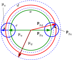
Figure 1: Phase space for DU processes with massless quarks

The relation between the Fermi momentum and the chemical potential in the Landau Fermi liquid theory can be derived from

$$\frac{\partial\mu}{\partial n} = \frac{2\pi^{2}}{d_{g}\mu p_{F}}+f_{0}^{S}-\frac{1}{3}f_{1}^{S},$$ (2)

where $d_{g}=2N_{f}N_{c}$ is the quark degeneracy factor and $N_{f}$ the number of flavors. $n$ is the number density of quasi-particles. The Landau coefficients $f_{0,1}^{S}$ are defined by

$$f_{l}^{S} \equiv \frac{2l+1}{4}\sum_{\sigma\sigma^{\prime}}\int\frac{d\Omega}{4\pi}P_{l}(\cos\theta)f_{\mathbf{p}\sigma,\mathbf{p}^{\prime}\sigma^{\prime}}.$$ (3)

Here $f_{\mathbf{p}\sigma,\mathbf{p}^{\prime}\sigma^{\prime}}$ is the Landau Fermi interaction for quarks with spin indices $\sigma$ and $\sigma^{\prime}$. The angle $\theta$ is between $\mathbf{p}$ and $\mathbf{p}^{\prime}$ both taken on the Fermi surface. The integral is over all directions of $\mathbf{p}$. The factor $1/4$ arises from the average over $\sigma$ and $\sigma^{\prime}$. The factor $(2l+1)$ comes from the normalization condition for Legendre polynomials $\int dxP_{l}^{2}(x)=2/(2l+1)$. The density of states on the Fermi surface is given by

$$N(0)\equiv\int d\tau\delta(E_{\mathbf{p}\sigma}-\mu)=\frac{d_{g}p_{F}^{2}}{2\pi^{2}}\left(\frac{\partial p}{\partial E_{\mathbf{p}\sigma}}\right)_{p_{F}},$$ (4)

where $(\partial p/\partial E_{\mathbf{p}\sigma})_{p_{F}}$ is the inverse of the quasi-particle velocity on the Fermi surface. Note that we have assumed that the flavor dependence of the quark mass is weak and negligible, which is true for $\beta$ equilibrium where $\mu_{u}\approx\mu_{d}$, so we suppressed the flavor indices of the chemical potential $\mu$.

In QCD, the quark-quark scattering amplitude via one-gluon exchange is given by

$$\mathcal{A}_{QCD} = \frac{C_{F}}{4N_{f}N_{c}}g^{2}\frac{1}{E_{\mathbf{p}_{1}}E_{\mathbf{p}_{2}}}\frac{4m^{2}-2P_{1}\cdot P_{2}}{(P_{1}-P_{2})^{2}}.$$ (5)

An average over colors, flavors and spins in the initial state and a sum over all of them in the final state have been taken. Here $P_{1}=(E_{\mathbf{p}_{1}},\mathbf{p}_{1})$ and $P_{2}=(E_{\mathbf{p}_{2}},\mathbf{p}_{2})$ are on-shell 4-momenta of two colliding quarks respectively, $m$ is the quark mass, and $g$ is the coupling constant in QCD and $\alpha_{S}=g^{2}/(4\pi)$. The amplitude diverges at small scattering angles $\theta$ since $(P_{1}-P_{2})^{2}\approx-2p_{F}^{2}(1-\cos\theta)\rightarrow 0$ if $m\neq 0$. The Landau coefficients can be obtained by applying Eq. (3). Of course all Landau coefficients are divergent. However the combination $f_{0}^{S}-\frac{1}{3}f_{1}^{S}$ is finite,

$$f_{0}^{S}-\frac{1}{3}f_{1}^{S} = \int\frac{d\Omega}{4\pi}\mathcal{A}_{QCD}(1-\cos\theta)\approx\frac{C_{F}}{4N_{f}N_{c}}g^{2}\frac{1}{\mu^{2}}\left(1-\frac{m^{2}}{p_{F}^{2}}\right).$$

Here the momenta and energies are set to the Fermi momentum and the chemical potential respectively. Substituting the above expression into Eq. (2), one obtains

$$\frac{d_{g}}{2\pi^{2}}p_{F}^{2}\frac{dp_{F}}{d\mu}=\left[\frac{2\pi^{2}}{d_{g}\mu p_{F}}+\frac{C_{F}g^{2}}{2d_{g}}\frac{1}{\mu^{2}}\left(2-\frac{\mu^{2}}{p_{F}^{2}}\right)\right]^{-1}$$ (6)

where we have used $n=\frac{d_{g}}{6\pi^{2}}p_{F}^{3}$. We assume $\alpha_{S}$ is small. The Fermi momentum is related to the chemical potential in the form

$$p_{F}=\mu(1-\kappa),$$ (7)

where $\kappa$ is the Fermi momentum reduction coefficient with respect to $\mu$ and is assumed to be a small dimensionless number. Then the solution of Eq. (6) reads

$$\kappa(\mu) = \left[\kappa(\mu_{0})-\frac{C_{F}\alpha_{S}}{2\pi}\right]\frac{\mu_{0}^{2}}{\mu^{2}}+\frac{C_{F}\alpha_{S}}{2\pi},$$ (8)

where we only kept the leading contribution. One can see in Eq. (8) the quark mass term belongs to the next-to-leading order and does not appear. The Fermi momentum reduction coefficient $\kappa(\mu)$ in Eq. (8) is illustrated in Fig. 2. There are two unconnected branches in $\kappa(\mu)$, one is above the static solution $\kappa=\frac{C_{F}\alpha_{S}}{2\pi}$, the other below it. For the upper branch, $\kappa(\mu)$ monotonously decreases and approaches the limit vaule $\kappa=\frac{C_{F}\alpha_{S}}{2\pi}$ with increasing $\mu$. For the lower branch, the trend is opposite. Both branches go towards the limit $\kappa=\frac{C_{F}\alpha_{S}}{2\pi}$ at asymptotically large $\mu$, i.e. $\kappa(\mu\rightarrow\infty)=\frac{C_{F}\alpha_{S}}{2\pi}$. But at lower $\mu$ or lower baryon densities, there are two different trends for $\kappa(\mu)$, one corresponds to more phase space and the other to less phase space for neutrino emissions.

If $\kappa$ is small and its dependence on $\mu$ is weak, Eq. (6) can be simplified to an algebraic equation without assuming $\alpha_{S}$ is small. The solution is

$$\kappa = \frac{C_{F}\alpha_{S}}{2\pi+5C_{F}\alpha_{S}}.$$ (9)

The above solution is lower than the limit value $\kappa(\mu\rightarrow\infty)=\frac{C_{F}\alpha_{S}}{2\pi}$ and can approach it when $\alpha_{S}\ll 1$. It is interesting to compare the solution (8) with (9). If near a specific value $\mu_{0}$ the dependence of $\kappa$ on the chemical potential is negligible, $\kappa(\mu_{0})$ is given by Eq. (9) satisfying $\kappa(\mu_{0})<\frac{C_{F}\alpha_{S}}{2\pi}$, which leads to $\kappa(\mu)<\frac{C_{F}\alpha_{S}}{2\pi}$ for any values of $\mu$ following Eq. (8). Thus the lower branch of the solutions in Fig. 2 is physical, implying quenched phase space for neutrnio emissions at lower baryon densities.

One can also determine from Eq. (7) and (8) the effective quark mass $m\sim\mu\sqrt{2\kappa}$ which is proportional to the chemical potential. Note that the effective quark mass is determined by the interquark interaction on the Fermi surface and can be much larger than the current quark mass.

Figure 2: The Fermi momentum reduction coefficient $\kappa(\mu)$ as given in Eq. (8). The dotted line is the static solution $\kappa=\frac{C_{F}\alpha_{S}}{2\pi}$. The solid line is the branch of $\kappa(\mu)$ below the dotted line corresponding to an initial value smaller than $\frac{C_{F}\alpha_{S}}{2\pi}$, while the dashed line is that above it. (a) With the initial value $\kappa(\mu_{0}=0.3)=\frac{C_{F}\alpha_{S}}{2\pi}\pm 0.08$; (b) with $\kappa(\mu_{0}=0.3)=\frac{C_{F}\alpha_{S}}{2\pi}\pm 0.1$. Following Eq. (9), the lower branch (solid line) is the physical solution.

The above results are from the QCD weak coupling approach and valid at very high densities. At mediate densities realized in neutron stars, one has to use more phenonmenological model like the NJL one. For a review of the NJL model in quark matter, see, e.g., Ref. Buballa:2003qv . Now we consider the simplest case in the NJL model, a two flavor system, whose Lagrangian is

$$\mathcal{L} = \overline{\psi}\left[i\gamma^{\mu}\partial_{\mu}-m\right]\psi+G_{S}\left[(\overline{\psi}\psi)^{2}+(\overline{\psi}i\gamma_{5}\bm{\tau}\psi)^{2}\right]-G_{V}(\overline{\psi}\gamma_{\mu}T^{a}\psi)^{2},$$ (10)

where $T^{a}=\lambda^{a}/2$ and $\lambda^{a}$ are the Gell-mann matrices in color space. $\bm{\tau}=(\tau^{1},\tau^{2},\tau^{3})$ are Pauli matrices in flavor space. $G_{S}$ is the coupling constant for the scalar and pseudoscalar channel, and $G_{V}$ is that for the vector channel. In some sense, these two channels are independent of each other. Hereafter we study each channel separately by setting the coupling constant zero in the other channel.

To obtain Landau coefficients $f_{0,1}^{S}$, we calculate the quark-quark scattering amplitude,

$$\mathcal{A} = \mathcal{A}_{S}+\mathcal{A}_{PS}+\mathcal{A}_{V}=\frac{1}{N_{f}N_{c}}\frac{B_{1}P_{1}\cdot P_{2}-B_{2}m^{2}}{E_{\mathbf{p}_{1}}E_{\mathbf{p}_{2}}},$$ (11)

where $B_{1}$ and $B_{2}$ are two coefficients depending on coupling constants $G_{S}$ and $G_{V}$,

$$B_{1} = 2G_{S}+C_{F}G_{V},$$

$$B_{2} = G_{S}(2N_{c}N_{f}+1)+2C_{F}G_{V}.$$ (12)

The amplitudes $\mathcal{A}_{S}$, $\mathcal{A}_{PS}$ and $\mathcal{A}_{V}$ for scalar, pseudoscalar and vector couplings respectively are given by

$$\mathcal{A}_{S} = \frac{1}{2N_{f}N_{c}}G_{S}\frac{P_{1}\cdot P_{2}-(4N_{c}N_{f}-1)m^{2}}{E_{\mathbf{p}_{1}}E_{\mathbf{p}_{2}}},$$

$$\mathcal{A}_{PS} = \frac{3}{2N_{f}N_{c}}G_{S}\frac{P_{1}\cdot P_{2}-m^{2}}{E_{\mathbf{p}_{1}}E_{\mathbf{p}_{2}}},$$

$$\mathcal{A}_{V} = \frac{C_{F}}{N_{f}N_{c}}G_{V}\frac{P_{1}\cdot P_{2}-2m^{2}}{E_{\mathbf{p}_{1}}E_{\mathbf{p}_{2}}}.$$ (13)

An average over colors, flavors and spins in the initial state and a sum over all of them in the final state have been taken. The Landau coefficients can be obtained by using Eq. (3),

$$f_{0} = \int\frac{d\Omega}{4\pi}\mathcal{A}=\frac{1}{N_{f}N_{c}}\left(B_{1}-B_{2}\frac{m^{2}}{\mu^{2}}\right),$$

$$f_{1} = 3\int\frac{d\Omega}{4\pi}\mathcal{A}\cos\theta=-\frac{B_{1}}{N_{f}N_{c}}\frac{p_{F}^{2}}{\mu^{2}},$$ (14)

where the momenta and energies are set to the Fermi momentum and the chemical potential respectively. Substituting $f_{0,1}^{S}$ of Eq. (14) into Eq. (2), using $n=\frac{d_{g}}{6\pi^{2}}p_{F}^{3}$, one obtains

$$\frac{d_{g}}{2\pi^{2}}p_{F}^{2}\frac{dp_{F}}{d\mu} = \left[\frac{2\pi^{2}}{d_{g}\mu p_{F}}+\frac{2}{d_{g}}\left(B_{1}-B_{2}+\left(\frac{1}{3}B_{1}+B_{2}\right)\frac{p_{F}^{2}}{\mu^{2}}\right)\right]^{-1}.$$ (15)

If we make the assumption $B_{1,2}\mu^{2}/\pi^{2}\sim B_{1,2}p_{F}^{2}/\pi^{2}\sim\kappa\ll 1$ (actually it is a good approximation for realistic values of $B_{1}$, but not so good for $B_{2}$) together with all other assumptions in solving Eq. (6), we get an analytical solution for $\kappa$,

$$\kappa(\mu) = \left[\kappa(\mu_{0})-\frac{2B_{1}\mu^{2}}{3\pi^{2}}\right]\frac{\mu_{0}^{2}}{\mu^{2}}+\frac{2B_{1}\mu^{2}}{3\pi^{2}},$$ (16)

which is in a similar form to Eq. (8). The solutions of $\kappa(\mu)$ also have two branches in analogy to the solutions of Eq. (8) shown in Fig. (2). We will argue that the lower branch $\kappa(\mu)<\frac{2B_{1}\mu^{2}}{3\pi^{2}}$ is favored, the same situation as in the QCD case.

If $\kappa$ is small and independent of $\mu$, one can solve Eq. (15) without the assumption $B_{1,2}\mu^{2}/\pi^{2}\ll 1$, similar to the QCD case,

$$\kappa = \frac{2B_{1}\mu^{2}}{3\pi^{2}+(7B_{1}+3B_{2})\mu^{2}}.$$ (17)

Since we have assumed that $\kappa$ is independent of $\mu$, $B_{1,2}\mu^{2}$ should be constants. The above solution is smaller than the limit value $\frac{2B_{1}\mu^{2}}{3\pi^{2}}$ of $\kappa(\mu)$ in Eq. (16) and recovers it when $B_{1,2}\mu^{2}/\pi^{2}\ll 1$. Therefore we have $\kappa(\mu)<\frac{2B_{1}\mu^{2}}{3\pi^{2}}$ for any values of $\mu$ following Eq. (16). Therefore both the QCD and NJL cases give the consistent trend of $\kappa(\mu)$ as monotonously increasing functions of $\mu$ towards their limit values at high densities.

We will use Eq. (17) in our forthcoming calculations. The effective mass on the Fermi surface is given by $m\sim\mu\sqrt{2\kappa}$. In the scalar and pseudoscalar channel, we set $G_{S}=5.1\times 10^{-6}\>\mathrm{MeV}^{-2}$, $\mu=500\>\mathrm{MeV}$ (these parameters are the same as in Ref. Ruster:2005jc ), then we obtain $\kappa\approx 0.052$ and $m\approx 160\>\mathrm{MeV}$. In the vector channel for $G_{V}=4.5\times 10^{-5}\>\mathrm{MeV}^{-2}$, one obtains $\kappa\approx 0.13$ and $m\approx 250\>\mathrm{MeV}$. In both channels, the effective quark masses are much larger than the current mass but much smaller than $\mu$.

From Eq. (8) or (17), one also obtains the angles between $u$ quark and electron momenta and between those of $u$ and $d$ quarks on the Fermi surface,

$$\cos\theta_{ue}\approx 1-\kappa,\;\cos\theta_{ud}\approx 1-\kappa\frac{\mu_{e}^{2}}{p_{Fu}p_{Fd}}.$$ (18)

These formula are useful in deriving neutrino emissivities in DU processes.

A few remarks are in order. All the results in this section apply to DU processes in normal and color superconducting quark matter. When calculating the quark-quark scattering amplitude, we do not take into account the fact that the chemical potentials for $u$ and $d$ quarks are different, the same approximation is also made in deriving Eq. (1) in QCD Baym:1975va ; Schafer:2004jp . In deriving Eq. (7), (8) and (17), we have made the approximation that $p_{F}\sim\mu$. This is consistent to the assumption that the effective quark mass is much smaller than the chemical potential. In this paper we take this assumption and use Eq. (17) in forthcoming calculations of neutrino emissivities. We find in the weak coupling regime the solutions for the Fermi momentum reduction coefficient $\kappa$ as monotonously increasing functions of chemical potential in the QCD and NJL cases. Such a trend in chemical potential implies that the phase space for neutrino emissions is quenched at lower baryon densities. This property seems robust and independent of specific models used in computing the Landau coefficients. In general case where $p_{F}\sim\mu$ does not hold, Eq. (7) is still valid but $\kappa$ has to be solved self-consistently. All the results in this section are for light quarks. If one takes into account strange quarks, the situation becomes much more complicated and one has to reformulate the whole Fermi liquid theory. This amounts to dealing with not only scatterings among strange quarks, but also those between light and strange quarks. A new Fermi liquid theory with two different Fermi surfaces is necessary.

III Quark propagators in a spin-one color superconductor

To obtain the neutrino emissivity in a spin-one color superconductor, we calculate the imaginary part of the $W$ boson polarization tensor from the superconducting quark loop, which involves the quark propagator $S(K)$. To obtain $S(K)$, we start from $S^{-1}(K)$ as follows

$$S^{-1}(K) = \left(\begin{array}[]{cc}S_{11}^{-1}&S_{12}^{-1}\\ S_{21}^{-1}&S_{22}^{-1}\end{array}\right)=\left(\begin{array}[]{cc}P_{\mu}\gamma^{\mu}+\mu_{f}\gamma_{0}-m&\phi_{f}\gamma_{0}\mathcal{M}_{\mathbf{k}}^{\dagger}\gamma_{0}\\ \phi_{f}\mathcal{M}_{\mathbf{k}}&P_{\mu}\gamma^{\mu}-\mu_{f}\gamma_{0}-m\end{array}\right),$$ (23)

where $\mathcal{M}_{\mathbf{k}}=\Delta_{il}\bm{\gamma}_{\bot}^{i}(\mathbf{k})J_{l}$ and $\gamma_{0}\mathcal{M}_{\mathbf{k}}^{\dagger}\gamma_{0}=\Delta_{il}^{*}\bm{\gamma}_{\bot}^{i}(\mathbf{k})J_{l}$ are $12\times 12$ gap matrices in color and Dirac space. $\mu_{f}$ is the chemical potential for quarks of the flavor $f$. $\phi_{f}$ is the magnitude of the gap. The form of $\Delta_{il}$ defines a specific spin-one phase, see Table I of Ref. Schmitt:2005wg for $\Delta_{il}$ in various phases. Here $\bm{\gamma}_{\bot}(\mathbf{k})\equiv\bm{\gamma}-\widehat{\mathbf{k}}(\widehat{\mathbf{k}}\cdot\bm{\gamma})$ are transverse Dirac matrices perpendicular to a momentum direction $\widehat{\mathbf{k}}$, and $J_{l}$ are generators of $SO(3)$ algebra with elements $(J_{l})_{ij}=i\epsilon^{ilj}$ with the anti-symmetric tensor $\epsilon^{ilj}$. As in Ref. Schmitt:2005wg , we only study transverse phases.

The structure of $\mathcal{M}_{\mathbf{k}}$ in Eq. (23) looks like in the massless case, but it is different actually. In the massless case $S_{21}^{-1}$ is expanded in terms of massless energy projectors $\Lambda_{\mathbf{k},m=0}^{e}$ [put $m=0$ in Eq. (49)] as $S_{21}^{-1}=\Lambda_{\mathbf{k},m=0}^{e}\phi_{f}^{e}\mathcal{M}_{\mathbf{k}}$. The expansion is justified by the fact that $\Lambda_{\mathbf{k},m=0}^{e}$ is commutable with $\gamma_{5}$ and $\bm{\gamma}_{\bot}^{i}(\mathbf{k})$. In the massive case the energy projectors $\Lambda_{\mathbf{k}}^{e}$ defined in Eq. (49) are not commutable with $\gamma_{5}$ and $\bm{\gamma}_{\bot}(\mathbf{k})$. So if one still assumes the same form of the gap matrix, the propagators and the dispersion relations would be much involved as are manifested in Ref. Aguilera:2005tg ; Aguilera:2006cj .

The propagator $S(K)$ is found by taking the inverse of $S^{-1}(K)$ in Eq. (23), see Appendix A for the derivation. One then obtains a very transparent form of the dispersion relations,

$$\epsilon_{\mathbf{k},r,f}^{e}=\sqrt{(\mu_{f}-eE_{k})^{2}+\lambda_{\mathbf{k},r}\phi_{f}^{2}},$$ (24)

where $E_{k}=\sqrt{k^{2}+m^{2}}$. $\lambda_{\mathbf{k},r}$ denote eigenvalues of the matrix $\gamma_{0}\mathcal{M}_{\mathbf{k}}^{\dagger}\mathcal{M}_{\mathbf{k}}\gamma_{0}$ given in Table I of Ref. Schmitt:2005wg for various phases. The gaps in a specific phase are given by $\sqrt{\lambda_{\mathbf{k},r}}\phi_{f}$. This form is the same as in the massless case except that $k$ is replaced by $E_{k}$. The results for $S_{11}$ and $S_{22}$ are given in Eq. (50) and (51). Since only quasi-particles are relevant in neutrino processes, we only keep excitations of positive energy, the branch with $e=+$, in $S_{11}$ and $S_{22}$. Then we have

$$S_{11/22} = \frac{k_{0}\mp\mu_{f}\pm E_{k}}{k_{0}^{2}-\epsilon_{\mathbf{k},r,f}^{2}}\mathcal{P}_{\mathbf{k},r}^{\pm}\Lambda_{\mathbf{k}}^{\pm}\gamma_{0},$$

where we have suppressed the superscript $e=+$ in the quasi-particle energy, $\epsilon_{\mathbf{k},r,f}\equiv\epsilon_{\mathbf{k},r,f}^{+}$. The projectors $\mathcal{P}_{\mathbf{k},r}^{\pm}$ are given in Eq. (52).

IV Time derivative of the neutrino distribution function

Our starting point to compute the neutrino emissivity is the time derivative of the neutrino distribution function derived from the Kadanoff-Baym equation for DU processes $u+e^{-}\rightarrow d+\nu$ and $d\rightarrow u+e^{-}+\overline{\nu}$. The procedure can be found in subsection A of section II in Ref. Schmitt:2005wg . The derivation of Kadanoff-Baym equation can also be found in various papers using closed time path formalism Sedrakian:1999jh ; Wang:2001dm ; Wang:2002qe . The result is

$$\frac{\partial}{\partial t}f_{\nu}(t,\mathbf{p}_{\nu}) = \frac{G_{F}^{2}}{4}\int\frac{d^{3}\mathbf{p}_{e}}{(2\pi)^{3}p_{\nu}p_{e}}L_{\lambda\sigma}(\mathbf{p}_{e},\mathbf{p}_{\nu})n_{F}(p_{e}-\mu_{e})n_{B}(p_{\nu}+\mu_{e}-p_{e})\mathrm{Im}\Pi_{R}^{\lambda\sigma}(Q).$$ (25)

Here $n_{F/B}(x)\equiv 1/(e^{x}\pm 1)$ are Fermi or Bose distribution functions. $f_{\nu}(t,\mathbf{p}_{\nu})$ is the neutrino (including the anti-neutrino contribution) distribution function. $\mathbf{p}_{e},\mathbf{p}_{\nu}$ are electron and neutrino momenta respectively. $\mu_{e}$ is the chemical potential for electrons. $G_{F}$ is the Fermi coupling constant. The leptonic tensor $L_{\lambda\sigma}(\mathbf{p}_{e},\mathbf{p}_{\nu})$ is given by

$$L_{\lambda\sigma}(\mathbf{p}_{e},\mathbf{p}_{\nu}) = \mathrm{Tr}\left[\gamma_{\lambda}(1-\gamma^{5})\gamma_{\mu}P_{e}^{\mu}\gamma_{\sigma}(1-\gamma^{5})\gamma_{\rho}P_{\nu}^{\rho}\right]$$ (26)

$$= 8\left(i\epsilon_{\lambda\sigma P_{e}P_{\nu}}+P_{\lambda}^{\nu}P_{\sigma}^{e}+P_{\sigma}^{\nu}P_{\lambda}^{e}-g_{\lambda\sigma}P_{e}\cdot P_{\nu}\right),$$

where $P_{e}$ and $P_{\nu}$ are on-shell 4-momenta. We have used the notation $\epsilon_{\lambda\sigma P_{e}P_{\nu}}\equiv\epsilon_{\lambda\sigma\eta\tau}P_{e}^{\eta}P_{\nu}^{\tau}$ with $\epsilon_{\lambda\sigma\eta\tau}$ the anti-symmetric tensor. $\Pi_{R}^{\lambda\sigma}(Q)$ is the retarded self-energy for $W$ bosons with a superconducting quark loop, where $Q=(p_{e}-\mu_{e}-p_{\nu},\mathbf{p}_{e}-\mathbf{p}_{\nu})$.

V Imaginary part of of the W-boson polarization tensor

Having quark propagators, we can calculate the imaginary part of the W-boson polarization tensor. Following the same procedure as in Ref. Schmitt:2005wg , one arrives at the following expression,

$$\mathrm{Im}\Pi_{R}^{\lambda\sigma}(Q) = \frac{T}{V}\mathrm{Im}\sum_{K}\sum_{r,s}\frac{1}{4E_{k}E_{p}}\left\{\frac{[k_{0}-\mu_{u}+E_{k}][p_{0}-\mu_{d}+E_{p}]}{(k_{0}^{2}-\epsilon_{\mathbf{k},r,u}^{2})(p_{0}^{2}-\epsilon_{\mathbf{p},s,d}^{2})}\mathcal{T}_{rs,+}^{\lambda\sigma}(\widehat{\mathbf{k}},\widehat{\mathbf{p}})\right.$$ (27)

$$\left.+\frac{[k_{0}+\mu_{d}-E_{k}][p_{0}+\mu_{u}-E_{p}]}{(k_{0}^{2}-\epsilon_{\mathbf{k},r,d}^{2})(p_{0}^{2}-\epsilon_{\mathbf{p},s,u}^{2})}\mathcal{T}_{rs,-}^{\lambda\sigma}(\widehat{\mathbf{k}},\widehat{\mathbf{p}})\right\}.$$

Here we used $P=K+Q$. The quark tensor $\mathcal{T}_{rs,\pm}^{\lambda\sigma}$ involves color and Dirac traces

$$\mathcal{T}_{rs,\pm}^{\lambda\sigma}(\widehat{\mathbf{k}},\widehat{\mathbf{p}}) \equiv 4E_{k}E_{p}\mathrm{Tr}\left[\gamma^{\lambda}(1\mp\gamma_{5})\mathcal{P}_{\mathbf{k},r}^{\pm}\Lambda_{\mathbf{k}}^{\pm}\gamma^{0}\gamma^{\sigma}(1\mp\gamma_{5})\mathcal{P}_{\mathbf{p},s}^{\pm}\Lambda_{\mathbf{p}}^{\pm}\gamma^{0}\right].$$ (28)

The negative component $\mathcal{T}_{rs,-}^{\lambda\sigma}$ can be related to the positive one $\mathcal{T}_{rs,+}^{\lambda\sigma}$ through Eq. (32). We can rewrite $\mathcal{T}_{rs,+}^{\lambda\sigma}(\widehat{\mathbf{k}},\widehat{\mathbf{p}})$ as

$$\mathcal{T}_{rs,+}^{\lambda\sigma}(\widehat{\mathbf{k}},\widehat{\mathbf{p}}) = \mathrm{Tr}\left[\gamma^{\lambda}(1-\gamma_{5})\mathcal{P}_{\mathbf{k},r}^{+}(\gamma_{\mu}K^{\mu})\gamma^{\sigma}(1-\gamma_{5})\mathcal{P}_{\mathbf{p},s}^{+}(\gamma_{\nu}P^{\nu})\right],$$ (29)

where we have dropped all mass terms which are vanishing. One sees that $\gamma_{\mu}K^{\mu}$ and $\gamma_{\nu}P^{\nu}$ appear in $\mathcal{T}_{rs,+}^{\lambda\sigma}(\widehat{\mathbf{k}},\widehat{\mathbf{p}})$, where $K^{\mu}$ and $P^{\nu}$ are on-shell quark momenta. In normal quark matter, one of the projectors, say $\mathcal{P}_{\mathbf{k},r=1}^{+}$ can be set to 1 and others with $r\neq 1$ set to zero, then one reproduces the result in the normal phase,

$$\mathcal{T}^{\lambda\sigma}(K,P) \equiv \mathrm{Tr}\left[\gamma^{\lambda}(1-\gamma_{5})(\gamma_{\mu}K^{\mu})\gamma^{\sigma}(1-\gamma_{5})(\gamma_{\nu}P^{\nu})\right]$$ (30)

$$= 8\left(i\epsilon^{\lambda\sigma KP}+P^{\lambda}K^{\sigma}+P^{\sigma}K^{\lambda}-g^{\lambda\sigma}K\cdot P\right).$$

Note that the anomalous propagators $S_{21}$ and $S_{12}$ containing the $uu$ and $dd$ condensates do not contribute to the self-energy. This is in contrast to spin-zero color superconductors, such as the 2SC and CFL phases, in which the anomalous propagators are off-diagonal in flavor space. This difference is related to the conservation of electric charge. Performing the Mastubara sum, one can extract the imaginary part,

$$\mathrm{Im}\Pi_{R}^{\lambda\sigma}(Q) = -\pi\sum_{r,s}\sum_{e_{1},e_{2}}\int\frac{d^{3}\mathbf{k}}{(2\pi)^{3}}\frac{1}{4E_{k}E_{p}}$$ (31)

$$\times\left[\mathcal{T}_{rs,+}^{\lambda\sigma}(\widehat{\mathbf{k}},\widehat{\mathbf{p}})B_{\mathbf{k},r,u}^{e_{1}}B_{\mathbf{p},s,d}^{e_{2}}\frac{n_{F}(-e_{1}\epsilon_{\mathbf{k},r,u})n_{F}(e_{2}\epsilon_{\mathbf{p},s,d})}{n_{B}(-e_{1}\epsilon_{\mathbf{k},r,u}+e_{2}\epsilon_{\mathbf{p},s,d})}\delta(q_{0}-e_{1}\epsilon_{\mathbf{k},r,u}+e_{2}\epsilon_{\mathbf{p},s,d})\right.$$

$$\left.+\mathcal{T}_{rs,-}^{\lambda\sigma}(\widehat{\mathbf{k}},\widehat{\mathbf{p}})B_{\mathbf{k},r,d}^{e_{1}}B_{\mathbf{p},s,u}^{e_{2}}\frac{n_{F}(e_{1}\epsilon_{\mathbf{k},r,d})n_{F}(-e_{2}\epsilon_{\mathbf{p},s,u})}{n_{B}(e_{1}\epsilon_{\mathbf{k},r,d}-e_{2}\epsilon_{\mathbf{p},s,u})}\delta(q_{0}+e_{1}\epsilon_{\mathbf{k},r,d}-e_{2}\epsilon_{\mathbf{p},s,u})\right],$$

where $q_{0}=p_{e}-\mu_{e}-p_{\nu}$. The Bogoliubov coefficients are defined by

$$B_{\mathbf{k},r,f}^{e} = \frac{\epsilon_{\mathbf{k},r,f}+e(\mu_{f}-E_{k})}{2\epsilon_{\mathbf{k},r,f}},$$

with $f=u,d$ and $e=\pm$. The two terms inside the square brackets are charge-conjugate of each other and give the same result. To see this, one changes the summation indices $e_{1}\leftrightarrow e_{2},$$r\leftrightarrow s$ in the second term, introduces the new integral variable $\mathbf{k}\rightarrow-\mathbf{k}-\mathbf{q}=-\mathbf{p}$ (also means $\mathbf{p}=\mathbf{k}+\mathbf{q}\rightarrow-\mathbf{k}$), and uses

$$\mathcal{T}_{sr,-}^{\lambda\sigma}(-\widehat{\mathbf{p}},-\widehat{\mathbf{k}}) = \mathcal{T}_{rs,+}^{\lambda\sigma}(\widehat{\mathbf{k}},\widehat{\mathbf{p}}).$$ (32)

The proof of the above identity for all phases considered in this paper is given in Appendix B. Taking into account $\lambda_{\mathbf{k},r}=\lambda_{-\mathbf{k},r}$ and then $\epsilon_{\mathbf{k},r,f}=\epsilon_{-\mathbf{k},r,f}$, we end up with the first term in Eq. (31). So we can keep the first term in Eq. (31) and double the result,

$$\mathrm{Im}\Pi_{R}^{\lambda\sigma}(Q) = -2\pi\sum_{r,s}\sum_{e_{1},e_{2}}\int\frac{d^{3}\mathbf{k}}{(2\pi)^{3}}\frac{1}{4E_{k}E_{p}}\mathcal{T}_{rs,+}^{\lambda\sigma}(\widehat{\mathbf{k}},\widehat{\mathbf{p}})B_{\mathbf{k},r,u}^{e_{1}}B_{\mathbf{p},s,d}^{e_{2}}$$ (33)

$$\times\frac{n_{F}(-e_{1}\epsilon_{\mathbf{k},r,u})n_{F}(e_{2}\epsilon_{\mathbf{p},s,d})}{n_{B}(-e_{1}\epsilon_{\mathbf{k},r,u}+e_{2}\epsilon_{\mathbf{p},s,d})}\delta(q_{0}-e_{1}\epsilon_{\mathbf{k},r,u}+e_{2}\epsilon_{\mathbf{p},s,d}).$$

VI Quark mass corrections to Neutrino emissivity

In this section we will calculate neutrino emissivities with massive quarks and identify the mass corrections. We will use the effective quark mass $m\sim\mu\sqrt{2\kappa}$ given in Sect. II. The effective quark mass is formed on the Fermi surface by the interquark interaction in the Landau Fermi liquid. Normally the effective quark mass is much larger than the current mass, but it is still small compared to the large chemical potential.

Inserting $\mathrm{Im}\Pi_{R}^{\lambda\sigma}(Q)$ in Eq. (33) back into Eq. (25), one obtains

$$\frac{\partial}{\partial t}f_{\nu}(t,\mathbf{p}_{\nu}) = -\frac{\pi}{8}G_{F}^{2}\int\frac{d^{3}\mathbf{p}}{(2\pi)^{3}p_{\nu}p_{e}}\int\frac{d^{3}\mathbf{k}}{(2\pi)^{3}E_{k}E_{p}}\sum_{r,s}\sum_{e_{1},e_{2}}L_{\lambda\sigma}(\mathbf{p}_{e},\mathbf{p}_{\nu})\mathcal{T}_{rs,+}^{\lambda\sigma}(\widehat{\mathbf{k}},\widehat{\mathbf{p}})B_{\mathbf{k},r,u}^{e_{1}}B_{\mathbf{p},s,d}^{e_{2}}$$ (34)

$$\times n_{F}(p_{e}-\mu_{e})n_{F}(-e_{1}\epsilon_{\mathbf{k},r,u})n_{F}(e_{2}\epsilon_{\mathbf{p},s,d})\delta(q_{0}-e_{1}\epsilon_{\mathbf{k},r,u}+e_{2}\epsilon_{\mathbf{p},s,d}),$$

where we have replaced the integral over $\mathbf{p}_{e}$ with that over $\mathbf{p}$. In normal quark matter, the quark tensor $\mathcal{T}^{\lambda\sigma}$ in Eq. (30) contracts with the leptonic tensor $L_{\lambda\sigma}$ in Eq. (26) giving the matrix element of the DU processes

$$\mathcal{T}^{\lambda\sigma}L_{\lambda\sigma} = |M|^{2},$$ (35)

with $|M|^{2}=256(P_{e}\cdot K)(P_{\nu}\cdot P)$. Using Eq. (7) and (18), the matrix element $|M|^{2}$ can be worked out,

$$|M|^{2} \approx 512\kappa E_{k}E_{p}p_{e}p_{\nu}\left[1-(1-\kappa)\cos\theta_{d\nu}\right],$$ (36)

with $\kappa$ given in Eq. (17).

The quark tensor $\mathcal{T}_{rs,+}^{\lambda\sigma}(\widehat{\mathbf{k}},\widehat{\mathbf{p}})$ in spin-one phases are evaluated in Appendix C. Using Eq. (53), its contraction with $L_{\lambda\sigma}$ is given by

$$L_{\lambda\sigma}\mathcal{T}_{rs,+}^{\lambda\sigma} = \omega_{rs}|M|^{2}+L_{\lambda\sigma}\delta\mathcal{T}_{rs}^{\lambda\sigma}.$$ (37)

Here the values of $\omega_{rs}$ are the same as in the massless case (see Tab. II of Ref. Schmitt:2005wg or Appendix C). As is shown in Appendix C, the dominant contribution in $\delta\mathcal{T}_{rs}^{\lambda\sigma}$ is from the term proportional to $R_{k}\mathcal{T}^{\lambda\sigma}(\widetilde{K}_{0},P)$ with $R_{k}\equiv(E_{k}-k)/k\approx m^{2}/(2p_{Fu}^{2})\sim\kappa$ and $\widetilde{K}_{0}\equiv(k,-\mathbf{k})$, because $P_{e}\cdot\widetilde{K}_{0}\sim 2p_{e}k$ is much larger than $P_{e}\cdot K\sim 2\kappa E_{k}p_{e}$. So $\delta\mathcal{T}_{rs}^{\lambda\sigma}$ can be written as $\delta\mathcal{T}_{rs}^{\lambda\sigma}\approx\chi_{rs}R_{k}\mathcal{T}^{\lambda\sigma}(\widetilde{K}_{0},P)$ where $\chi_{rs}$ is listed in Tab. 1. Terms of $R_{p}\mathcal{T}^{\lambda\sigma}(K,\widetilde{P}_{0})\sim\kappa m^{2}/p_{Fd}^{2}\sim\kappa^{2}$ are next to leading order since the appearance of $\widetilde{P}_{0}$ does not enhance the order of magnitude of the result, so they are suppressed by $\kappa$ compared to the massless term. Also terms of $R_{k}R_{p}\mathcal{T}^{\lambda\sigma}(\widetilde{K}_{0},\widetilde{P}_{0})\sim m^{4}/(p_{Fu}^{2}p_{Fd}^{2})\sim\kappa^{2}$ are also suppressed due to double $R$ factors. Explicitly one derives

$$L_{\lambda\sigma}\delta\mathcal{T}_{rs}^{\lambda\sigma} \approx \chi_{rs}\frac{m^{2}}{2p_{Fu}\mu_{u}}256E_{k}E_{p}p_{e}p_{\nu}\left[1-(1-\kappa)\cos\theta_{d\nu}\right],$$ (38)

$$\approx \chi_{rs}\frac{\kappa}{1-\kappa}256E_{k}E_{p}p_{e}p_{\nu}\left[1-(1-\kappa)\cos\theta_{d\nu}\right].$$

The term $\kappa\cos\theta_{d\nu}$ inside the square brackets can be dropped since it is of high order.

Let us understand Tab. 1. We find $\chi_{rs}=0$ for the polar phase. The reason is simple: all projectors (54) are in color space or decoupled from Dirac space, so the quark tensor $\mathcal{T}_{rs,+}^{\lambda\sigma}$ is proportional to $\mathcal{T}^{\lambda\sigma}$. For other phases, A, planar and CSL, color and Dirac indices are coupled. Thus with massive quarks, the Dirac structure of the quark tensor is more complicated. Taking the A phase for example, it is easy to understand $\chi_{rs}=0$ for $rs=13,31,23,32,33$, because the excitation branch 3 only involves the color blue while branch 1 and 2 involve colors red and green. One observes that $\chi_{12}=\chi_{21}\neq 0$ even in the collinear limit, meaning that there is an entanglement between two different branches. Remembering that the projectors of the A phase can be expressed in terms of helicity projectors, as shown in Eq. (60) of Ref. Schmitt:2005wg , quasiparticles of branch 1 have helicity +1 for $\widehat{k}_{3}<0$ and helicity -1 for $\widehat{k}_{3}>0$, while quasiparticles of branch 2 have opposite helicities. In the massless case, helicity means chirality. The DU processes only allow quarks with left chirality to participate. Therefore in the collinear limit $\widehat{k}_{3}\approx\widehat{p}_{3}$, different branches cannot crosstalk. However when quarks have masses, a helicity eigenstate is not chirality one. In an eigenstate of left chirality, one can find eigenstates of both helicities, which makes two different branches coupled together. In the same way, one can understand the appearance $\delta\mathcal{T}_{rs}^{\lambda\sigma}$ in the quark tensor with different structure from $\mathcal{T}^{\lambda\sigma}$. A projector of a spin-one phase can be expanded with respect to helicity projectors. In the massless case, the quark tensors for all branches have the same Dirac structure as in normal quark matter. With non-zero quark mass, this is no longer the case: new terms in the quark tensor emerge from an overlapping of subspace with different helicities (but with the same chirality). They have different structure and cannot be collected into $\mathcal{T}^{\lambda\sigma}$ as in the massless case. This can be seen from the fact that such terms as $\gamma_{0}\bm{\gamma}\cdot\widehat{\mathbf{k}}\gamma_{\mu}K^{\mu}$ or $\gamma_{\mu}K^{\mu}\bm{\gamma}\cdot\widehat{\mathbf{k}}\gamma_{0}$ appear inside the trace of Eq. (29) for A, planar and CSL phases,

$$\gamma_{0}\bm{\gamma}\cdot\widehat{\mathbf{k}}\gamma_{\mu}K^{\mu} = \gamma_{\mu}K^{\mu}(\bm{\gamma}\cdot\widehat{\mathbf{k}})\gamma_{0}=\gamma_{\mu}K^{\mu}-R_{k}\gamma_{\mu}\widetilde{K}_{0}^{\mu}.$$ (39)

When masses are zero, the result is just $\gamma_{\mu}K^{\mu}$, which results in traces proportional to $\mathcal{T}^{\lambda\sigma}$ in Eq. (30). When masses are non-zero, there is an additional term $R_{k}\gamma_{\mu}\widetilde{K}_{0}^{\mu}$ different from $\mathcal{T}^{\lambda\sigma}$.

Table 1: The values of $\chi_{rs}$ in quark mass term $\delta\mathcal{T}_{rs}^{\lambda\sigma}\approx\chi_{rs}R_{k}\mathcal{T}^{\lambda\sigma}(\widetilde{K}_{0},P)$. For the polar phase $\chi_{rs}=0$ for all $r$ and $s$. The row and column are labeled by $r$ and $s$ respectively. The collinear limit is taken. We used the notation $\xi\equiv\widehat{k}_{3}$ and $\theta(\xi)\equiv 1+\mathrm{sgn}(\xi)$ for the step function of $\xi$.

Planar	1	2
1	$-\frac{2\xi^{2}}{(1+\xi^{2})^{2}}$	$\frac{2\xi^{2}}{(1+\xi^{2})^{2}}$
2	$\frac{2\xi^{2}}{(1+\xi^{2})^{2}}$	$-\frac{2\xi^{2}}{(1+\xi^{2})^{2}}$

A	1	2	3
1	$-\theta(\xi)$	$\theta(-\xi)$	0
2	$\theta(\xi)$	$-\theta(-\xi)$	0
3	0	0	0

CSL	1	2
1	$-\frac{1}{2}$	$\frac{1}{2}$
2	$\frac{1}{2}$	$-\frac{1}{2}$

Using Eq. (34) and (38), the emissivity is written as a sum of two terms

$$\epsilon_{\nu} = -\int\frac{d^{3}\mathbf{p}_{\nu}}{(2\pi)^{3}}p_{\nu}\frac{\partial}{\partial t}f_{\nu}(t,\mathbf{p}_{\nu})\equiv\epsilon_{\nu}^{(0)}+\epsilon_{\nu}^{(1)}.$$ (40)

Here $\epsilon_{\nu}^{(0)}$ is in the same form as the emissivity in the massless case which we denote as $\epsilon_{\nu}^{(m=0)}$, i.e. Eq. (40) of Ref. Schmitt:2005wg , except that all $k$ and $p$ are replaced by $E_{k}$ and $E_{p}$ in dispersion relations respectively, and that $2\alpha_{S}/(3\pi)$ replaced by $\kappa$ in Eq. (8) or (17). It comes from the term $\omega_{rs}|M|^{2}$ in Eq. (37). In the massless case, the ranges of the integrals over $k-\mu_{u}$ and/or $p-\mu_{d}$ on which the quark distributions depend are $[-\mu_{u/d},\infty]$, which are further taken to be $[-\infty,\infty]$. With non-zero quark mass, the integrals over $k-\mu_{u}$ and/or $p-\mu_{d}$ have to be transformed to those over $E_{k/p}-\mu_{u/d}$ on which the quark distribution functions depend, i.e.

$$dpdk = (E_{p}E_{k}/pk)dE_{p}dE_{k}=(E_{k}E_{p}/pk)d(E_{p}-\mu)d(E_{k}-\mu)$$ (41)

$$\approx \frac{\mu_{u}\mu_{d}}{pk}d(E_{p}-\mu)d(E_{k}-\mu).$$

In the last equality we have chosen $E_{k}\approx\mu_{u}$ and $E_{p}\approx\mu_{d}$ on the Fermi surface. The range of $E_{k/p}-\mu_{u/d}$ becomes $[m-\mu_{u/d},\infty]$ and is further approximated to be $[-\infty,\infty]$ if $m\ll\mu_{u/d}$. Using Eq. (18), (34) and (37), we obtain

$$\epsilon_{\nu}^{(0)}=\epsilon_{\nu}^{(m=0)}.$$ (42)

This means $\epsilon_{\nu}^{(0)}$ is identical to the emissivity in the massless case.

The second part of the emissivity in Eq. (40), $\epsilon_{\nu}^{(1)}$, has obvious mass dependence. It comes from the term $L_{\lambda\sigma}\delta\mathcal{T}_{rs}^{\lambda\sigma}$ in Eq. (37). Inserting Eq. (38) into Eq. (34) and using Eq. (40), one obtains

$$\epsilon_{\nu}^{(1)} = 32\pi\frac{\kappa}{1-\kappa}G_{F}^{2}\mu_{e}\mu_{u}\mu_{d}\int\frac{d^{3}\mathbf{p}_{\nu}}{(2\pi)^{3}}p_{\nu}\int\frac{dE_{p}d\Omega_{\mathbf{p}}}{(2\pi)^{3}}\int\frac{dE_{k}d\Omega_{\mathbf{k}}}{(2\pi)^{3}}\sum_{r,s}\sum_{e_{1},e_{2}}\chi_{rs}(1-\cos\theta_{d\nu})$$ (43)

$$\times B_{\mathbf{k},r,u}^{e_{1}}B_{\mathbf{p},s,d}^{e_{2}}n_{F}(p_{e}-\mu_{e})n_{F}(-e_{1}\epsilon_{\mathbf{k},r,u})n_{F}(e_{2}\epsilon_{\mathbf{p},s,d})\delta[\cos\theta_{ud}-1+\kappa\mu_{e}^{2}/(p_{Fu}p_{Fd})],$$

where Eq. (41) was used in the integral. We have also used

$$\delta(p_{e}-\mu_{e}-p_{\nu}-e_{1}\epsilon_{\mathbf{k},r,u}+e_{2}\epsilon_{\mathbf{p},s,d}) \approx \frac{\mu_{e}}{p_{Fu}p_{Fd}}\delta[\cos\theta_{ud}-1+\kappa\mu_{e}^{2}/(p_{Fu}p_{Fd})].$$ (44)

After taking the same procedure as in Ref. Schmitt:2005wg , one has

$$\epsilon_{\nu}^{(1)} \approx \frac{1}{\pi^{5}}\frac{\kappa}{1-\kappa}G_{F}^{2}\mu_{e}\mu_{u}\mu_{d}T^{6}G^{\prime}(\varphi_{u},\varphi_{d}),$$ (45)

with integral $G^{\prime}$ defined by

$$G^{\prime}(\varphi_{u},\varphi_{d}) \equiv \sum_{e_{1},e_{2}}\sum_{r,s}\int_{-1}^{1}d\xi\chi_{rs}(\xi)\int_{0}^{\infty}dvv^{3}\int_{0}^{\infty}dx\int_{0}^{\infty}dy\;n_{F}(v+e_{1}\sqrt{y^{2}+\lambda_{r}(\xi)\varphi_{u}^{2}}-e_{2}\sqrt{x^{2}+\lambda_{s}(\xi)\varphi_{d}^{2}})$$ (46)

$$\times n_{F}(-e_{1}\sqrt{y^{2}+\lambda_{r}(\xi)\varphi_{u}^{2}})n_{F}(e_{2}\sqrt{x^{2}+\lambda_{s}(\xi)\varphi_{d}^{2}}).$$

Here we used dimensionless gaps scaled by the temperature, $\varphi_{u,d}\equiv\phi_{u,d}/T$. Eq. (45) shows that $\epsilon_{\nu}^{(1)}$ is in the same order as $\epsilon_{\nu}^{(m=0)}$. We can take the special case $\varphi_{u}=\varphi_{d}=\varphi$ and do the numerical calculation for $G^{\prime}$ as a function of $\varphi$. The results are shown in Fig. (3). We see that $G^{\prime}<0$ for all three spin-one phases. At asymptotically low temperature or large $\varphi$, $G^{\prime}$ for CSL and Planar phases approach constants due to the gapless mode 2,

$$G^{\prime}=-\frac{457\pi^{6}}{5040}\;\;(\mathrm{CSL}),\;-\frac{457\pi^{6}(\pi/2-1)}{5040}\;\;(\mathrm{Planar}).$$

For the A phase, $G^{\prime}$ turns to zero at large $\varphi$ since all contributions come from the gapped modes.

In summary, from Eq. (40), (42) and (45), the emissivity can be written as the sum of two terms,

$$\epsilon_{\nu}=\epsilon_{\nu}^{m=0}+\epsilon_{\nu}^{(1)},$$ (47)

where $\epsilon_{\nu}^{(1)}$ is the correction due to non-zero quark mass and it is of the same order as $\epsilon_{\nu}^{(m=0)}$. It is zero for the polar phase. For the CSL and Planar phases, we obtain

$$\epsilon_{\nu}^{(1)}\approx C_{i}\frac{1}{1-\kappa}\epsilon_{\nu}^{(m=0)}\sim C_{i}\epsilon_{\nu}^{(m=0)},\;\;i=\mathrm{A,\>CSL,\>Planar}$$

At asymptotically large $\varphi$, the coefficients $C_{i}$ are given by

$$C_{\mathrm{A}} = 0,\;\;C_{\mathrm{CSL}}=-\frac{1}{4}\approx-0.25,\;\;C_{\mathrm{Planar}}=-\frac{(\pi-2)}{8}\approx-0.15.$$ (48)

which show that mass corrections are about 25% (CSL) and 15% (Planar) of the contributions in the massless case at very low temperatures. These results are quite universal at $\kappa\ll 1$, which is the case for the weak coupling approach in QCD with one gluon exchange as $\kappa\sim\alpha_{S}$. This is also the case for the realistic values of coupling constants $G_{S}\sim 5.1\times 10^{-6}\>\mathrm{MeV}^{-2}$ and $G_{V}\sim 4.5\times 10^{-5}\>\mathrm{MeV}^{-2}$ in the NJL model which give $\kappa\sim 0.05-0.13$.

Figure 3: $G^{\prime}$ versus $\varphi$ for spin-one phases.

A few comments are in order. The gap matrix in Eq. (23) leads to the same form of the dispersion relations as in the massless case. This much facilitates the calculation with transparency. If the gap matrix is not in this form, the dispersion relation is more involved Aguilera:2005tg ; Aguilera:2006cj . But one can prove that they are equivalent in some limits (see the discussion in section VII of Ref. Schmitt:2005wg ). We have used the collinear limit, where the momentum direction of $u$ quarks is almost the same as that of $d$ quarks. The effective quark mass $m\sim\mu\sqrt{2\kappa}$ is also used in the calculation, which is much larger than the current mass but small compared to the chemical potential. Then we find that the mass corrections to the emissivity are of the same order as in the massless case. The mass corrections from gapless modes in CSL and Planar phases which are dominant at low temperatures are about 25% and 15% of the contributions in the massless case respectively. These percentages for the mass corrections are universal as long as $\kappa\ll 1$. The mass corrections could be very different near the chiral phase transition and for the DU processes with strange quarks with even larger quark mass. However the current formulation is only valid at small mass limit compared to the chemical potential. For very large quark mass, the Landau Fermi liquid theory has to be reformulated and the integral in the emissivity is very different from the massless case since the integral range $E-\mu$ cannot literally be taken as $[-\infty,\infty]$ due to $m\sim\mu$. Not only this has to be modified, one also has to deal with scatterings between light and strange quarks, which involves the Fermi liquid theory with two different Fermi surfaces. This is beyond the scope of the current work and deserves a future study.

Appendix A Energy projectors and propagators

We make use of energy projectors to get $S(K)$ from $S^{-1}(K)$ in Eq. (23). The energy projectors are given by

$$\Lambda_{\mathbf{k}}^{e} = \frac{1}{2}\left[1+e\frac{\gamma_{0}(\bm{\gamma}\cdot\mathbf{k}+m)}{E_{k}}\right],$$ (49)

where $E_{k}=\sqrt{k^{2}+m^{2}}$. We can express $S_{11}^{-1}$ and $S_{22}^{-1}$ in terms of energy projectors:

$$S_{11/22}^{-1}=(k_{0}\pm\mu_{f}-eE_{k})\gamma_{0}\Lambda_{\mathbf{k}}^{e}.$$

The chemical potential $\mu_{f}$ has flavor index $f$. The elements of $S(K)$ are given by

$$S_{11} = \left[S_{11}^{-1}-S_{12}^{-1}(S_{22}^{-1})^{-1}S_{21}^{-1}\right]^{-1},$$

$$S_{22} = \left[S_{22}^{-1}-S_{21}^{-1}(S_{11}^{-1})^{-1}S_{12}^{-1}\right]^{-1},$$

$$S_{21} = -(S_{22}^{-1})^{-1}S_{21}^{-1}S_{11},$$

$$S_{12} = -(S_{11}^{-1})^{-1}S_{12}^{-1}S_{22}.$$

To get $S_{11}$, we need to evaluate

$$S_{12}^{-1}(S_{22}^{-1})^{-1}S_{21}^{-1} = \phi_{f}^{2}\gamma_{0}\alpha_{\bot}^{i}(\mathbf{k})\Delta_{il}^{*}J_{l}(S_{22}^{-1})^{-1}\gamma_{0}\alpha_{\bot}^{i^{\prime}}(\mathbf{k})\Delta_{i^{\prime}l^{\prime}}J_{l^{\prime}}$$

$$= \phi_{f}^{2}\gamma_{0}[\alpha_{\bot}^{i}(\mathbf{k})\Delta_{il}^{*}J_{l}][\alpha_{\bot}^{i^{\prime}}(\mathbf{k})\Delta_{i^{\prime}l^{\prime}}J_{l^{\prime}}]\frac{1}{k_{0}-\mu_{f}-eE_{k}}\Lambda_{\mathbf{k}}^{-e}.$$

Here we have used $\Lambda_{\mathbf{k}}^{e}\alpha_{\bot}^{i}(\mathbf{k})=\alpha_{\bot}^{i}(\mathbf{k})\Lambda_{\mathbf{k}}^{-e}$ with $\bm{\alpha}=\gamma_{0}\bm{\gamma}$. Note that

$$L_{\mathbf{k}}^{+}\equiv[\alpha_{\bot}^{i}(\mathbf{k})\Delta_{il}^{*}J_{l}][\alpha_{\bot}^{i^{\prime}}(\mathbf{k})\Delta_{i^{\prime}l^{\prime}}J_{l^{\prime}}]$$

is just the matrix $\gamma_{0}\mathcal{M}_{\mathbf{k}}^{\dagger}\mathcal{M}_{\mathbf{k}}\gamma_{0}$ in Eq. (14) of Ref. Schmitt:2005wg , and it is commutable with $\Lambda_{\mathbf{k}}^{e}$. We can decompose $L_{\mathbf{k}}^{+}$ in terms of its projectors as $L_{\mathbf{k}}^{+}=\lambda_{\mathbf{k},r}\mathcal{P}_{\mathbf{k},r}^{+}$. Then we obtain

$$S_{11} = \frac{k_{0}-\mu_{f}+eE_{k}}{k_{0}^{2}-(\epsilon_{\mathbf{k},r,f}^{e})^{2}}\mathcal{P}_{\mathbf{k},r}^{+}\Lambda_{\mathbf{k}}^{e}\gamma_{0},$$ (50)

with the quasi-particle excitation energy $\epsilon_{\mathbf{k},r,f}^{e}=\sqrt{(\mu-eE_{k})^{2}+\lambda_{\mathbf{k},r}\phi_{f}^{2}}$.

Making the change $\mu_{f}\rightarrow-\mu_{f}$ in $S_{11}$, we get $S_{22}$

$$S_{22}=\frac{k_{0}+\mu_{f}-eE_{k}}{k_{0}^{2}-(\epsilon_{\mathbf{k},r,f}^{e})^{2}}\mathcal{P}_{\mathbf{k},r}^{-}\Lambda_{\mathbf{k}}^{-e}\gamma_{0},$$ (51)

where $\mathcal{P}_{\mathbf{k},r}^{-}$ are projectors of

$$L_{\mathbf{k}}^{-}\equiv[\alpha_{\bot}^{i}(\mathbf{k})\Delta_{il}J_{l}][\alpha_{\bot}^{i^{\prime}}(\mathbf{k})\Delta_{i^{\prime}l^{\prime}}^{*}J_{l^{\prime}}],$$

whose eigenvalues $\lambda_{\mathbf{k},r}$ are the same as $L_{\mathbf{k}}^{+}$’s. The projectors $\mathcal{P}_{\mathbf{k},r}^{\pm}$ are given by

$$\mathcal{P}_{\mathbf{k},t}^{\pm} = \prod_{r\neq t}\frac{L_{\mathbf{k}}^{\pm}-\lambda_{\mathbf{k},r}}{\lambda_{\mathbf{k},t}-\lambda_{\mathbf{k},r}}.$$ (52)

Note that the projectors $\mathcal{P}_{\mathbf{k},r}^{\pm}$ are commutable with $\Lambda_{\mathbf{k}}^{e}$ since $[L_{\mathbf{k}}^{\pm},\Lambda_{\mathbf{k}}^{e}]=0$.

Appendix B Proof of the identity (32)

One starts from $\mathcal{T}_{rs,-}^{\lambda\sigma}$ as follows

$$\mathcal{T}_{sr,-}^{\lambda\sigma}(-\widehat{\mathbf{p}},-\widehat{\mathbf{k}})=\mathrm{Tr}\left[\gamma^{\lambda}(1+\gamma_{5})\mathcal{P}_{-\mathbf{p},s}^{-}\Lambda_{-\mathbf{p}}^{-}\gamma^{0}\gamma^{\sigma}(1+\gamma_{5})\mathcal{P}_{-\mathbf{k},r}^{-}\Lambda_{-\mathbf{k}}^{-}\gamma^{0}\right].$$

Inserting the charge conjugate operator $C=i\gamma_{0}\gamma^{2}$ and using $C\alpha^{i}\alpha^{j}C^{-1}=(\alpha^{j}\alpha^{i})^{T}$, $\alpha_{\bot}^{i}(-\mathbf{k})=\alpha_{\bot}^{i}(\mathbf{k})$ and $J_{l}=-J_{l}^{T}$, one obtains

$$C\mathcal{P}_{-\mathbf{k},r}^{-}C^{-1} = (\mathcal{P}_{\mathbf{k},r}^{+})^{T}.$$

One uses $C\gamma^{\mu}C^{-1}=-\gamma^{\mu T}$ to obtain

$$C\Lambda_{-\mathbf{p}}^{-}\gamma^{0}C^{-1} = (\Lambda_{\mathbf{p}}^{+}\gamma^{0})^{T}.$$

Also one has $C\gamma_{5}C^{-1}=\gamma_{5}=\gamma_{5}^{T}$. Then one finally arrives at

$$\mathcal{T}_{sr,-}^{\lambda\sigma}(-\widehat{\mathbf{p}},-\widehat{\mathbf{k}}) = \mathrm{Tr}\left[\gamma^{\lambda T}(1+\gamma_{5})^{T}(\mathcal{P}_{\mathbf{p},s}^{+})^{T}(\Lambda_{\mathbf{p}}^{+}\gamma^{0})^{T}\gamma^{\sigma T}(1+\gamma_{5})^{T}(\mathcal{P}_{\mathbf{k},r}^{+})^{T}(\Lambda_{\mathbf{k}}^{+}\gamma^{0})^{T}\right]$$

$$= \mathrm{Tr}\left[\gamma^{\lambda}(1-\gamma_{5})\Lambda_{\mathbf{k}}^{+}\gamma^{0}\mathcal{P}_{\mathbf{k},r}^{+}\gamma^{\sigma}(1-\gamma_{5})\Lambda_{\mathbf{p}}^{+}\gamma^{0}\mathcal{P}_{\mathbf{p},r}^{+}\right]^{T}$$

$$= \mathrm{Tr}\left[\gamma^{\lambda}(1-\gamma_{5})\mathcal{P}_{\mathbf{k},r}^{+}\Lambda_{\mathbf{k}}^{+}\gamma^{0}\gamma^{\sigma}(1-\gamma_{5})\mathcal{P}_{\mathbf{p},s}^{+}\Lambda_{\mathbf{p}}^{+}\gamma^{0}\right]$$

$$= \mathcal{T}_{rs,+}^{\lambda\sigma}(\widehat{\mathbf{k}},\widehat{\mathbf{p}}),$$

where $[\mathcal{P}_{\mathbf{k},r}^{+},\Lambda_{\mathbf{k}}^{+}\gamma^{0}]=0$ has been used.

Appendix C Calculate quark tensor $\mathcal{T}_{rs,+}^{\lambda\sigma}$ for spin-one phases

The quark tensor $\mathcal{T}_{rs,+}^{\lambda\sigma}$ can be written as a sum of the leading term with the same structure as in the massless case and the mass correction term,

$$\mathcal{T}_{rs,+}^{\lambda\sigma}(\widehat{\mathbf{k}},\widehat{\mathbf{p}}) = \omega_{rs}\mathcal{T}^{\lambda\sigma}(K,P)+\delta\mathcal{T}_{rs}^{\lambda\sigma},$$ (53)

where $\mathcal{T}^{\lambda\sigma}(K,P)$ is the quark tensor in the normal phase and given in Eq. (30). $\delta\mathcal{T}_{rs}^{\lambda\sigma}$ is the correction from the quark mass.

C.1 Polar phase

The polar phase is particularly simple. The order parameter or the condensate has the form

$$\mathcal{M}_{\mathbf{k}}=J_{3}\gamma_{\perp,3}(\widehat{\mathbf{k}}).$$

The projectors $\mathcal{P}_{\mathbf{k},r}^{+}$ do not depend on the quark momentum $\mathbf{k}$,

$$\mathcal{P}_{\mathbf{k},1}^{+} = J_{3}^{2},$$

$$\mathcal{P}_{\mathbf{k},2}^{+} = 1-J_{3}^{2}.$$ (54)

The trace can be decoupled into a color and a Dirac one. The color trace is

$$\mathrm{Tr}[\mathcal{P}_{\mathbf{k},1}^{+}\mathcal{P}_{\mathbf{k},1}^{+}] = 2,$$

$$\mathrm{Tr}[\mathcal{P}_{\mathbf{k},2}^{+}\mathcal{P}_{\mathbf{k},2}^{+}] = 1,$$

$$\mathrm{Tr}[\mathcal{P}_{\mathbf{k},1}^{+}\mathcal{P}_{\mathbf{k},2}^{+}] = 0.$$

The Dirac trace is the same as in the normal phase in Eq. (30). So we have

$$\omega_{11}=2,\;\omega_{22}=1,\;\omega_{12}=\omega_{21}=0,$$

$$\delta\mathcal{T}_{rs}^{\lambda\sigma}=0\;(r,s=1,2).$$

C.2 Planar phase

The order parameter is in the form

$$\mathcal{M}_{\mathbf{k}} = J_{1}\gamma_{\perp}^{1}(\widehat{\mathbf{k}})+J_{2}\gamma_{\perp}^{2}(\widehat{\mathbf{k}}).$$

The projectors are

$$\mathcal{P}_{\mathbf{k},1}^{+} = \frac{1}{1+\widehat{k}_{3}^{2}}\left[J_{1}^{2}(1-\widehat{k}_{1}^{2})+J_{2}^{2}(1-\widehat{k}_{2}^{2})-\{J_{1},J_{2}\}\widehat{k}_{1}\widehat{k}_{2}+J_{3}\widehat{k}_{3}\gamma_{0}\gamma^{5}\bm{\gamma}\cdot\widehat{\mathbf{k}}\right],$$

$$\mathcal{P}_{\mathbf{k},2}^{+} = 1-\mathcal{P}_{\mathbf{k},1}^{+}.$$

We can rewrite $\mathcal{P}_{\mathbf{k},1}^{+}$ and $\mathcal{P}_{\mathbf{k},2}^{+}$ in the form

$$\mathcal{P}_{\mathbf{k},1}^{+} = I_{1\mathbf{k}}+I_{2\mathbf{k}}\gamma_{0}\gamma^{5}\bm{\gamma}\cdot\widehat{\mathbf{k}},$$

$$\mathcal{P}_{\mathbf{k},2}^{+} = 1-I_{1\mathbf{k}}-I_{2\mathbf{k}}\gamma_{0}\gamma^{5}\bm{\gamma}\cdot\widehat{\mathbf{k}},$$

with

$$I_{1\mathbf{k}} = \frac{1}{1+\widehat{k}_{3}^{2}}\left[J_{1}^{2}(1-\widehat{k}_{1}^{2})+J_{2}^{2}(1-\widehat{k}_{2}^{2})-\{J_{1},J_{2}\}\widehat{k}_{1}\widehat{k}_{2}\right],$$

$$I_{2\mathbf{k}} = \frac{1}{1+\widehat{k}_{3}^{2}}J_{3}\widehat{k}_{3}.$$

We obtain

$$\omega_{11} = \mathrm{Tr}_{c}\left[I_{1\mathbf{k}}I_{1\mathbf{p}}\right]+\mathrm{Tr}_{c}\left[I_{2\mathbf{k}}I_{2\mathbf{p}}\right],$$

$$\omega_{22} = -1+\mathrm{Tr}_{c}\left[I_{1\mathbf{k}}I_{1\mathbf{p}}\right]+\mathrm{Tr}_{c}\left[I_{2\mathbf{k}}I_{2\mathbf{p}}\right],$$

$$\omega_{12} = \omega_{21}=2-\mathrm{Tr}_{c}\left[I_{1\mathbf{k}}I_{1\mathbf{p}}\right]-\mathrm{Tr}_{c}\left[I_{2\mathbf{k}}I_{2\mathbf{p}}\right],$$

$$\delta\mathcal{T}_{11}^{\lambda\sigma} = \mathrm{Tr}_{c}\left[I_{2\mathbf{k}}I_{2\mathbf{p}}\right]\left[-R_{p}\mathcal{T}^{\lambda\sigma}(K,\widetilde{P}_{0})-R_{k}\mathcal{T}^{\lambda\sigma}(\widetilde{K}_{0},P)+R_{p}R_{k}\mathcal{T}^{\lambda\sigma}(\widetilde{K}_{0},\widetilde{P}_{0})\right],$$

$$\delta\mathcal{T}_{22}^{\lambda\sigma} = \delta\mathcal{T}_{11}^{\lambda\sigma}=-\delta\mathcal{T}_{12}^{\lambda\sigma}=-\delta\mathcal{T}_{21}^{\lambda\sigma},$$

where $R_{k}=(E_{k}-k)/k$ , $K=(E_{k},\mathbf{k})$ and $\widetilde{K}_{0}=(k,-\mathbf{k})$. $\mathcal{T}^{\lambda\sigma}$ is given in Eq. (30). In the collinear limit, $\mathbf{k}\parallel\mathbf{p}$ or $\widehat{\mathbf{k}}\approx\widehat{\mathbf{p}}$, the color traces can be simplified, then we obtain

$$\omega_{11} = 2,\;\omega_{22}=1,\;\omega_{12}=\omega_{21}=0,$$

$$\delta\mathcal{T}_{11}^{\lambda\sigma} = \frac{2\widehat{k}_{3}^{2}}{(1+\widehat{k}_{3}^{2})^{2}}\left[-R_{p}\mathcal{T}^{\lambda\sigma}(K,\widetilde{P}_{0})-R_{k}\mathcal{T}^{\lambda\sigma}(\widetilde{K}_{0},P)+R_{p}R_{k}\mathcal{T}^{\lambda\sigma}(\widetilde{K}_{0},\widetilde{P}_{0})\right],$$

$$\delta\mathcal{T}_{22}^{\lambda\sigma} = \delta\mathcal{T}_{11}^{\lambda\sigma}=-\delta\mathcal{T}_{12}^{\lambda\sigma}=-\delta\mathcal{T}_{21}^{\lambda\sigma}.$$

C.3 $A$ phase

The order parameter is

$$\mathcal{M}_{\mathbf{k}} = J_{3}\left[\gamma_{\perp}^{1}(\widehat{\mathbf{k}})+i\gamma_{\perp}^{2}(\widehat{\mathbf{k}})\right].$$

The projectors are

$$\mathcal{P}_{\mathbf{k},1}^{+} = \frac{1}{2}J_{3}^{2}\left[1+\mathrm{sgn}(\widehat{k}_{3})\gamma_{0}\gamma^{5}\bm{\gamma}\cdot\widehat{\mathbf{k}}\right],$$

$$\mathcal{P}_{\mathbf{k},2}^{+} = \frac{1}{2}J_{3}^{2}\left[1-\mathrm{sgn}(\widehat{k}_{3})\gamma_{0}\gamma^{5}\bm{\gamma}\cdot\widehat{\mathbf{k}}\right],$$

$$\mathcal{P}_{\mathbf{k},3}^{+} = 1-J_{3}^{2},$$

where $\mathrm{sgn}(x)$ is the sign of $x$. The results for $\omega_{rs}$ are

$$\omega_{11} = \frac{1}{2}[1+\mathrm{sgn}(\widehat{k}_{3})][1+\mathrm{sgn}(\widehat{p}_{3})],$$

$$\omega_{22} = \frac{1}{2}[1-\mathrm{sgn}(\widehat{k}_{3})][1-\mathrm{sgn}(\widehat{p}_{3})],$$

$$\omega_{33} = 1,$$

$$\omega_{13} = \omega_{31}=\omega_{23}=\omega_{32}=0,$$

$$\omega_{12} = \frac{1}{2}[1+\mathrm{sgn}(\widehat{k}_{3})][1-\mathrm{sgn}(\widehat{p}_{3})],$$

$$\omega_{21} = \frac{1}{2}[1-\mathrm{sgn}(\widehat{k}_{3})][1+\mathrm{sgn}(\widehat{p}_{3})].$$

The results for $\delta\mathcal{T}_{rs}^{\lambda\sigma}$ are

$$\delta\mathcal{T}_{11}^{\lambda\sigma} = -\frac{1}{2}\mathrm{sgn}(\widehat{p}_{3})[1+\mathrm{sgn}(\widehat{k}_{3})]R_{p}\mathcal{T}^{\lambda\sigma}(K,\widetilde{P}_{0})$$

$$-\frac{1}{2}\mathrm{sgn}(\widehat{k}_{3})[1+\mathrm{sgn}(\widehat{p}_{3})]R_{k}\mathcal{T}^{\lambda\sigma}(\widetilde{K}_{0},P)$$

$$+\frac{1}{2}\mathrm{sgn}(\widehat{p}_{3})\mathrm{sgn}(\widehat{k}_{3})R_{p}R_{k}\mathcal{T}^{\lambda\sigma}(\widetilde{K}_{0},\widetilde{P}_{0}),$$

$$\delta\mathcal{T}_{22}^{\lambda\sigma} = \frac{1}{2}\mathrm{sgn}(\widehat{p}_{3})[1-\mathrm{sgn}(\widehat{k}_{3})]R_{p}\mathcal{T}^{\lambda\sigma}(K,\widetilde{P}_{0})$$

$$+\frac{1}{2}\mathrm{sgn}(\widehat{k}_{3})[1-\mathrm{sgn}(\widehat{p}_{3})]R_{k}\mathcal{T}^{\lambda\sigma}(\widetilde{K}_{0},P)$$

$$+\frac{1}{2}\mathrm{sgn}(\widehat{p}_{3})\mathrm{sgn}(\widehat{k}_{3})R_{p}R_{k}\mathcal{T}^{\lambda\sigma}(\widetilde{K}_{0},\widetilde{P}_{0}),$$

$$\delta\mathcal{T}_{33}^{\lambda\sigma} = \delta\mathcal{T}_{13}^{\lambda\sigma}=\delta\mathcal{T}_{31}^{\lambda\sigma}=\delta\mathcal{T}_{23}^{\lambda\sigma}=\delta\mathcal{T}_{32}^{\lambda\sigma}=0,$$

$$\delta\mathcal{T}_{12}^{\lambda\sigma} = \frac{1}{2}\mathrm{sgn}(\widehat{p}_{3})[1+\mathrm{sgn}(\widehat{k}_{3})]R_{p}\mathcal{T}^{\lambda\sigma}(K,\widetilde{P}_{0})$$

$$-\frac{1}{2}\mathrm{sgn}(\widehat{k}_{3})[1-\mathrm{sgn}(\widehat{p}_{3})]R_{k}\mathcal{T}^{\lambda\sigma}(\widetilde{K}_{0},P)$$

$$-\frac{1}{2}\mathrm{sgn}(\widehat{p}_{3})\mathrm{sgn}(\widehat{k}_{3})R_{p}R_{k}\mathcal{T}^{\lambda\sigma}(\widetilde{K}_{0},\widetilde{P}_{0}),$$

$$\delta\mathcal{T}_{21}^{\lambda\sigma} = -\frac{1}{2}\mathrm{sgn}(\widehat{p}_{3})[1-\mathrm{sgn}(\widehat{k}_{3})]R_{p}\mathcal{T}^{\lambda\sigma}(K,\widetilde{P}_{0})$$

$$+\frac{1}{2}\mathrm{sgn}(\widehat{k}_{3})[1+\mathrm{sgn}(\widehat{p}_{3})]R_{k}\mathcal{T}^{\lambda\sigma}(\widetilde{K}_{0},P)$$

$$-\frac{1}{2}\mathrm{sgn}(\widehat{p}_{3})\mathrm{sgn}(\widehat{k}_{3})R_{p}R_{k}\mathcal{T}^{\lambda\sigma}(\widetilde{K}_{0},\widetilde{P}_{0}).$$

In the collinear limit $\widehat{\mathbf{k}}\approx\widehat{\mathbf{p}}$, we have

$$\omega_{11}=2\theta(\widehat{k}_{3}),\;\omega_{22}=2\theta(-\widehat{k}_{3}),\;\omega_{33}=1,$$

$$\omega_{12}=\omega_{21}=\omega_{13}=\omega_{31}=\omega_{23}=\omega_{32}=0,$$

and

$$\delta\mathcal{T}_{11}^{\lambda\sigma} = -\theta(\widehat{k}_{3})R_{p}\mathcal{T}^{\lambda\sigma}(K,\widetilde{P}_{0})-\theta(\widehat{k}_{3})R_{k}\mathcal{T}^{\lambda\sigma}(\widetilde{K}_{0},P)+\frac{1}{2}R_{p}R_{k}\mathcal{T}^{\lambda\sigma}(\widetilde{K}_{0},\widetilde{P}_{0}),$$

$$\delta\mathcal{T}_{22}^{\lambda\sigma} = -\theta(-\widehat{k}_{3})R_{p}\mathcal{T}^{\lambda\sigma}(K,\widetilde{P}_{0})-\theta(-\widehat{k}_{3})R_{k}\mathcal{T}^{\lambda\sigma}(\widetilde{K}_{0},P)+\frac{1}{2}R_{p}R_{k}\mathcal{T}^{\lambda\sigma}(\widetilde{K}_{0},\widetilde{P}_{0}),$$

$$\delta\mathcal{T}_{33}^{\lambda\sigma} = \delta\mathcal{T}_{13}^{\lambda\sigma}=\delta\mathcal{T}_{31}^{\lambda\sigma}=\delta\mathcal{T}_{23}^{\lambda\sigma}=\delta\mathcal{T}_{32}^{\lambda\sigma}=0,$$

$$\delta\mathcal{T}_{12}^{\lambda\sigma} = \theta(\widehat{k}_{3})R_{p}\mathcal{T}^{\lambda\sigma}(K,\widetilde{P}_{0})+\theta(-\widehat{k}_{3})R_{k}\mathcal{T}^{\lambda\sigma}(\widetilde{K}_{0},P)-\frac{1}{2}R_{p}R_{k}\mathcal{T}^{\lambda\sigma}(\widetilde{K}_{0},\widetilde{P}_{0}),$$

$$\delta\mathcal{T}_{21}^{\lambda\sigma} = \theta(-\widehat{k}_{3})R_{p}\mathcal{T}^{\lambda\sigma}(K,\widetilde{P}_{0})+\theta(\widehat{k}_{3})R_{k}\mathcal{T}^{\lambda\sigma}(\widetilde{K}_{0},P)-\frac{1}{2}R_{p}R_{k}\mathcal{T}^{\lambda\sigma}(\widetilde{K}_{0},\widetilde{P}_{0}),$$

where $\theta(x)\equiv 1+\mathrm{sgn}(x)$ is the step function.

C.4 CSL phase

The order parameter is

$$\mathcal{M}_{\mathbf{k}} = \mathbf{J}\cdot\bm{\gamma}_{\perp}(\widehat{\mathbf{k}}).$$

The projectors are

$$\mathcal{P}_{\mathbf{k},1}^{+} = -\frac{1}{2}\left[\mathbf{J}\cdot\bm{\gamma}\right]^{2},$$

$$\mathcal{P}_{\mathbf{k},2}^{+} = 1+\frac{1}{2}\left[\mathbf{J}\cdot\bm{\gamma}\right]^{2}.$$

It is convenient to rewrite these projectors in terms of color indices,

$$(\mathcal{P}_{\mathbf{k},1}^{+})_{ab} = \delta_{ab}+\frac{1}{2}\gamma_{\bot}^{b}\gamma_{\bot}^{a},$$

$$(\mathcal{P}_{\mathbf{k},2}^{+})_{ab} = -\frac{1}{2}\gamma_{\bot}^{b}\gamma_{\bot}^{a}.$$

We obtain

$$\omega_{11} = 1+\frac{1}{4}\left[1+(\widehat{\mathbf{k}}\cdot\widehat{\mathbf{p}})^{2}+2(\widehat{\mathbf{k}}\cdot\widehat{\mathbf{p}})\right],$$

$$\omega_{22} = \frac{1}{4}\left[1+(\widehat{\mathbf{k}}\cdot\widehat{\mathbf{p}})^{2}+2(\widehat{\mathbf{k}}\cdot\widehat{\mathbf{p}})\right],$$

$$\omega_{12} = \omega_{21}=1-\frac{1}{4}\left[1+(\widehat{\mathbf{k}}\cdot\widehat{\mathbf{p}})^{2}+2(\widehat{\mathbf{k}}\cdot\widehat{\mathbf{p}})\right],$$

and

$$\delta\mathcal{T}_{11}^{\lambda\sigma} = \frac{1}{2}(\widehat{\mathbf{k}}\cdot\widehat{\mathbf{p}})\left[-R_{p}\mathcal{T}^{\lambda\sigma}(K,\widetilde{P}_{0})-R_{k}\mathcal{T}^{\lambda\sigma}(\widetilde{K}_{0},P)+R_{p}R_{k}\mathcal{T}^{\lambda\sigma}(\widetilde{K}_{0},\widetilde{P}_{0})\right],$$

$$\delta\mathcal{T}_{22}^{\lambda\sigma} = \delta\mathcal{T}_{11}^{\lambda\sigma}=-\delta\mathcal{T}_{12}^{\lambda\sigma}=-\delta\mathcal{T}_{21}^{\lambda\sigma}.$$

In the collinear limit, we have

$$\omega_{11}=2,\;\omega_{22}=1,\;\omega_{12}=\omega_{21}=0,$$

$$\delta\mathcal{T}_{11}^{\lambda\sigma}=\frac{1}{2}\left[-R_{p}\mathcal{T}^{\lambda\sigma}(K,\widetilde{P}_{0})-R_{k}\mathcal{T}^{\lambda\sigma}(\widetilde{K}_{0},P)+R_{p}R_{k}\mathcal{T}^{\lambda\sigma}(\widetilde{K}_{0},\widetilde{P}_{0})\right],$$

$$\delta\mathcal{T}_{22}^{\lambda\sigma}=\delta\mathcal{T}_{11}^{\lambda\sigma}=-\delta\mathcal{T}_{12}^{\lambda\sigma}=-\delta\mathcal{T}_{21}^{\lambda\sigma}.$$

References

- (1) N. Itoh, Prog. Theor. Phys. 44, 291 (1970).
- (2) J. C. Collins and M. J. Perry, Phys. Rev. Lett. 34, 1353 (1975).
- (3) B. C. Barrois, Nucl. Phys. B 129, 390 (1977).
- (4) D. Bailin and A. Love, Phys. Rept. 107, 325 (1984).
- (5) M. G. Alford, K. Rajagopal and F. Wilczek, Phys. Lett. B 422, 247 (1998) [arXiv:hep-ph/9711395].
- (6) M. G. Alford, K. Rajagopal and F. Wilczek, Nucl. Phys. B 537, 443 (1999) [arXiv:hep-ph/9804403].
- (7) R. Rapp, T. Schafer, E. V. Shuryak and M. Velkovsky, Phys. Rev. Lett. 81, 53 (1998) [arXiv:hep-ph/9711396].
- (8) D. T. Son, Phys. Rev. D 59, 094019 (1999) [arXiv:hep-ph/9812287].
- (9) R. D. Pisarski and D. H. Rischke, Phys. Rev. D 61, 074017 (2000) [arXiv:nucl-th/9910056].
- (10) D. K. Hong, V. A. Miransky, I. A. Shovkovy and L. C. R. Wijewardhana, Phys. Rev. D 61, 056001 (2000) [Erratum-ibid. D 62, 059903 (2000)] [arXiv:hep-ph/9906478].
- (11) K. Rajagopal and F. Wilczek, arXiv:hep-ph/0011333.
- (12) M. G. Alford, Ann. Rev. Nucl. Part. Sci. 51, 131 (2001) [arXiv:hep-ph/0102047].
- (13) S. Reddy, Acta Phys. Polon. B 33, 4101 (2002)[arXiv:nucl-th/0211045].
- (14) R. Casalbuoni and G. Nardulli, Rev. Mod. Phys. 76, 263 (2004) [arXiv:hep-ph/0305069].
- (15) T. Schafer, arXiv:hep-ph/0304281.
- (16) D. H. Rischke, Prog. Part. Nucl. Phys. 52, 197 (2004) [arXiv:nucl-th/0305030].
- (17) M. Buballa, Phys. Rept. 407, 205 (2005) [arXiv:hep-ph/0402234].
- (18) H. c. Ren, arXiv:hep-ph/0404074.
- (19) I. A. Shovkovy, Found. Phys. 35, 1309 (2005) [arXiv:nucl-th/0410091].
- (20) W. E. Brown, J. T. Liu and H. c. Ren, Phys. Rev. D 61, 114012 (2000) [arXiv:hep-ph/9908248].
- (21) Q. Wang and D. H. Rischke, Phys. Rev. D 65, 054005 (2002) [arXiv:nucl-th/0110016].
- (22) A. Schmitt, Q. Wang and D. H. Rischke, Phys. Rev. D 66, 114010 (2002) [arXiv:nucl-th/0209050].
- (23) A. Ipp, A. Gerhold and A. Rebhan, Phys. Rev. D 69, 011901 (2004) [arXiv:hep-ph/0309019].
- (24) P. T. Reuter, Q. Wang and D. H. Rischke, Phys. Rev. D 70, 114029 (2004) [Erratum-ibid. D 71, 099901 (2005)] [arXiv:nucl-th/0405079].
- (25) A. Gerhold and A. Rebhan, Phys. Rev. D 71, 085010 (2005) [arXiv:hep-ph/0501089].
- (26) J. L. Noronha, H. c. Ren, I. Giannakis, D. Hou and D. H. Rischke, arXiv:hep-ph/0602218.
- (27) Q. Wang, J. Phys. G 30, S1251 (2004) [arXiv:nucl-th/0404017].
- (28) A. Rebhan, arXiv:hep-ph/0504023.
- (29) A. Gerhold, arXiv:hep-ph/0503279.
- (30) A. Gerhold, A. Ipp and A. Rebhan, arXiv:hep-ph/0512273.
- (31) P. T. Reuter, arXiv:nucl-th/0602043.
- (32) K. Iida and G. Baym, Phys. Rev. D 63, 074018 (2001) [Erratum-ibid. D 66, 059903 (2002)] [arXiv:hep-ph/0011229].
- (33) M. Alford and K. Rajagopal, JHEP 0206, 031 (2002) [arXiv:hep-ph/0204001].
- (34) A. W. Steiner, S. Reddy and M. Prakash, Phys. Rev. D 66, 094007 (2002) [arXiv:hep-ph/0205201].
- (35) M. Huang, P. f. Zhuang and W. q. Chao, Phys. Rev. D 67, 065015 (2003) [arXiv:hep-ph/0207008].
- (36) F. Neumann, M. Buballa and M. Oertel, Nucl. Phys. A 714, 481 (2003) [arXiv:hep-ph/0210078].
- (37) S. B. Ruster and D. H. Rischke, Phys. Rev. D 69, 045011 (2004) [arXiv:nucl-th/0309022].
- (38) M. Huang and I. A. Shovkovy, Phys. Rev. D 70, 051501 (2004) [arXiv:hep-ph/0407049].
- (39) R. Casalbuoni, R. Gatto, M. Mannarelli, G. Nardulli and M. Ruggieri, Phys. Lett. B 605, 362 (2005) [Erratum-ibid. B 615, 297 (2005)] [arXiv:hep-ph/0410401].
- (40) I. Giannakis and H. C. Ren, Phys. Lett. B 611, 137 (2005) [arXiv:hep-ph/0412015].
- (41) M. Alford and Q. h. Wang, J. Phys. G 31, 719 (2005) [arXiv:hep-ph/0501078].
- (42) K. Fukushima, Phys. Rev. D 72, 074002 (2005) [arXiv:hep-ph/0506080].
- (43) K. Rajagopal and A. Schmitt, Phys. Rev. D 73, 045003 (2006) [arXiv:hep-ph/0512043].
- (44) I. Giannakis and H. C. Ren, Nucl. Phys. B 723, 255 (2005) [arXiv:hep-th/0504053].
- (45) E. V. Gorbar, M. Hashimoto and V. A. Miransky, Phys. Lett. B 632, 305 (2006) [arXiv:hep-ph/0507303].
- (46) T. Schafer, Phys. Rev. Lett. 96, 012305 (2006) [arXiv:hep-ph/0508190].
- (47) M. Kitazawa, D. H. Rischke and I. A. Shovkovy, arXiv:hep-ph/0602065.
- (48) L. He, M. Jin and P. Zhuang, arXiv:hep-ph/0604224.
- (49) T. Schafer, Phys. Rev. D 62, 094007 (2000) [arXiv:hep-ph/0006034].
- (50) M. G. Alford, J. A. Bowers, J. M. Cheyne and G. A. Cowan, Phys. Rev. D 67, 054018 (2003) [arXiv:hep-ph/0210106].
- (51) M. Buballa, J. Hosek and M. Oertel, Phys. Rev. Lett. 90, 182002 (2003) [arXiv:hep-ph/0204275].
- (52) A. Schmitt, Q. Wang and D. H. Rischke, Phys. Rev. Lett. 91, 242301 (2003) [arXiv:nucl-th/0301090].
- (53) A. Schmitt, Phys. Rev. D 71, 054016 (2005) [arXiv:nucl-th/0412033].
- (54) D. N. Aguilera, D. Blaschke, M. Buballa and V. L. Yudichev, Phys. Rev. D 72, 034008 (2005) [arXiv:hep-ph/0503288].
- (55) M. G. Alford and G. A. Cowan, J. Phys. G 32, 511 (2006) [arXiv:hep-ph/0512104].
- (56) D. Vollhardt and P. Wölfle, The Superfluid Phases of Helium 3 (Taylor & Francis, London, 1990).
- (57) S. Popov, H. Grigorian and D. Blaschke, arXiv:nucl-th/0512098.
- (58) A. Schmitt, I. A. Shovkovy and Q. Wang, Phys. Rev. D 73, 034012 (2006) [arXiv:hep-ph/0510347].
- (59) A. Schmitt, I. A. Shovkovy and Q. Wang, Phys. Rev. Lett. 94, 211101 (2005) [Erratum-ibid. 95, 159902(E) (2005)] [arXiv:hep-ph/0502166].
- (60) P. Jaikumar, C. D. Roberts and A. Sedrakian, Phys. Rev. C 73, 042801 (2006) [arXiv:nucl-th/0509093].
- (61) N. Iwamoto, Phys. Rev. Lett. 44 (1980) 1637.
- (62) G. Baym and S. A. Chin, Nucl. Phys. A 262, 527 (1976).
- (63) T. Schafer and K. Schwenzer, Phys. Rev. D 70, 114037 (2004) [arXiv:astro-ph/0410395].
- (64) D. N. Aguilera, D. Blaschke, H. Grigorian and N. N. Scoccola, arXiv:hep-ph/0604196.
- (65) S. B. Ruster, V. Werth, M. Buballa, I. A. Shovkovy and D. H. Rischke, Phys. Rev. D 72, 034004 (2005) [arXiv:hep-ph/0503184].
- (66) A. Sedrakian and A. Dieperink, Phys. Lett. B 463, 145 (1999) [arXiv:nucl-th/9905039].
- (67) Q. Wang, K. Redlich, H. Stoecker and W. Greiner, Phys. Rev. Lett. 88, 132303 (2002) [arXiv:nucl-th/0111040].
- (68) Q. Wang, K. Redlich, H. Stoecker and W. Greiner, Nucl. Phys. A 714, 293 (2003) [arXiv:hep-ph/0202165].