Limiting fragmentation in hadron-hadron
collisions at high energies

Abstract

Limiting fragmentation in proton-proton, deuteron-nucleus and nucleus-nucleus collisions is analyzed in the framework of the Balitsky-Kovchegov equation in high energy QCD. Good agreement with experimental data is obtained for a wide range of energies. Further detailed tests of limiting fragmentation at RHIC and the LHC will provide insight into the evolution equations for high energy QCD.

1. Service de Physique Théorique (URA 2306 du CNRS)
   CEA/DSM/Saclay, Bât. 774
   91191, Gif-sur-Yvette Cedex, France

2. Brookhaven National Laboratory,
   Physics Department, Nuclear Theory,
   Upton, NY-11973, USA

3. H. Niewodniczański Institute of Nuclear Physics,
   Polish Academy of Sciences,
   ul. Radzikowskiego 152, 31-342 Kraków, Poland

1 Introduction

The hypothesis of limiting fragmentation in high energy hadron-hadron collisions was suggested nearly four decades ago [1]. This hypothesis states that the produced particles, in the rest frame of one of the colliding hadrons, will approach a limiting distribution. These universal distributions describe the momentum distributions of the fragments of the other hadron. Central to the original hypothesis of the limiting fragmentation in Ref. [1] was the assumption that the total hadronic cross sections would become constant at large center-of-mass energy. If this occurred, the excitation and break-up of a hadron would be independent of the center-of-mass energy and distributions in the fragmentation region would approach a limiting curve.

We now know that the total hadronic cross-sections are not constant at high energies. Instead, to the highest energies achieved, they grow slowly with the center-of-mass energy $\sqrt{s}$, with favored functional forms being either a power law behavior $\sigma(s)\propto s^{\alpha}$ with $\alpha\approx 0.08$ [2] or a $\sigma(s)\propto\ln^{2}(s)$ [3]. A measurement of the total cross-section at the LHC [4] will further help constrain the possible functional forms.

Even though the cross-sections are not constant, limiting fragmentation appears to have a wide regime of validity. It was confirmed experimentally in $p\bar{p},pA,\pi A$ and nucleus-nucleus collisions at high energies [5, 6, 7, 8]. More recently, the BRAHMS and PHOBOS experiments at the Relativistic Heavy Ion Collider (RHIC) at Brookhaven National Laboratory (BNL) have performed detailed studies of the pseudo-rapidity distribution of the produced charged particles $dN_{\rm ch}/d\eta$ for a wide range ($-5.4<\eta<5.4$) of pseudo-rapidities, and for several center-of-mass energies ($\sqrt{s_{{}_{NN}}}=19.6,62.4,130\mbox{\ and\ }200\,{\rm GeV}$) in nucleus-nucleus (Au-Au and Cu-Cu) and deuteron-nucleus (d-Au) collisions. Results for pseudo-rapidity distributions have also been obtained over a limited kinematic range in pseudo-rapidity by the STAR experiment at RHIC [9]. These measurements in A-A and d-A collisions were performed for several centralities. In addition to the d-Au and A-A data, there are $pp$ data at $\sqrt{s}=200\;{\rm GeV}$ and also at $\sqrt{s}=410$ GeV. (In the near future, data at $\sqrt{s}=500$ GeV may become available.) These measurements have opened a new and precise window on many scaling phenomena glimpsed at lower energies. In particular, they have performed detailed studies of the limiting fragmentation phenomenon. The pseudo-rapidity distribution $\frac{dN}{d\eta^{\prime}}$ (where $\eta^{\prime}\equiv\eta-Y_{\rm beam}$ is the pseudo-rapidity shifted by the beam rapidity $y_{beam}=\ln\sqrt{s}/m_{p}$) is observed to become independent of the center-of-mass energy $\sqrt{s}$ in the region around $\eta^{\prime}\sim 0$

$$\frac{dN_{\rm ch}}{d\eta^{\prime}}(\eta^{\prime},\sqrt{s},b)\equiv\frac{dN_{\rm ch}}{d\eta^{\prime}}(\eta^{\prime},b)\;,$$ (1)

where $b$ is the impact parameter.

It is worth noting that this scaling is in a strong disagreement with boost invariant scenarios which predict a fixed fragmentation region and a broad central plateau growing with energy. It would therefore be desirable to understand the nature of hadronic interactions that lead to limiting fragmentation and the deviations away from it. In a recent article, Białas and Jeżabek [47], argued that some qualitative features of limiting fragmentation can be explained in a two-step model involving multiple gluon exchange between partons of the colliding hadrons and the subsequent radiation of hadronic clusters by the interacting hadrons. In this paper, we compute limiting fragmentation within the Color Glass Condensate (CGC) approach [14] to high energy hadronic collisions–its relation to the Białas-Jeżabek model will be addressed briefly later.

In the CGC formalism, gluon production in the limiting fragmentation region can be described, at leading order, in the framework of $k_{\perp}$-factorization. Under this assumption, the inclusive cross-section for produced gluons is expressed as the convolution of the “unintegrated parton distributions” in the projectile and target respectively ,

$$\phi_{{}_{A}}(x_{1},k_{1\perp}\equiv|{\boldsymbol{k}}_{1\perp}|)\;\phi_{{}_{B}}(x_{2},k_{2\perp}\equiv|{\boldsymbol{k}}_{2\perp}|)\;\delta^{(2)}({\boldsymbol{p}}_{\perp}-{\boldsymbol{k}}_{1\perp}-{\boldsymbol{k}}_{2\perp})\;,$$ (2)

times a (transverse momentum dependent) vertex squared. As we shall emphasize later, the name “unintegrated parton distributions” though conventional is somewhat imprecise because the objects $\phi_{{}_{A,B}}$ that enter in this formula differ from the expectation value of the gluon number operator. In eq. (2), $x_{1}$ and $x_{2}$ are the longitudinal momentum fractions of the gluons probed in the projectile and target, namely,

$$x_{1}\equiv{p_{\perp}\over m_{{}_{N}}}\,e^{y-Y_{\rm beam}}\;,\quad x_{2}\equiv{p_{\perp}\over m_{{}_{N}}}\,e^{-y-Y_{\rm beam}}\;,$$ (3)

where $Y_{\rm beam}\equiv\ln(\sqrt{s}/m_{{}_{N}})$ is the beam rapidity, $m_{{}_{N}}$ is the nucleon mass, and ${\boldsymbol{p}}_{\perp}={\boldsymbol{k}}_{1\perp}+{\boldsymbol{k}}_{2\perp}$ is the transverse momentum of the produced gluon. We should emphasize that the kinematics here is the $2\rightarrow 1$ eikonal kinematics, which provides the leading contribution to gluon production in the CGC picture.

As we will discuss further later, $k_{\perp}$-factorization actually works best in the limiting fragmentation kinematics where $x_{1}\geq 0.1$ and $x_{2}\ll 1$ (or vice versa). Clearly, $k_{\perp}$-factorization tells us that the cross-sections depend in general on both $y-Y_{\rm beam}$ and $y+Y_{\rm beam}$. However, target limiting fragmentation implies a dependence on solely $y-Y_{\rm beam}$ of the spectrum of produced particles integrated over the transverse momentum. As we shall see in section 2, such a scaling emerges in a straightforward manner in the $k_{\perp}$-factorization framework if a) the typical transverse momentum in the projectile is much smaller than the typical transverse momentum in the target, and b) if unitarity is preserved in the evolution of the target with $x_{2}$. These two conditions are naturally fulfilled in the CGC picture when $x_{2}$ becomes so small that the target reaches the “black disk” limit. More importantly, by studying how this limit is reached, one gets some insight into systematic deviations away from the limiting fragmentation.

The dynamical evolution of the unintegrated distributions with $x$ are described in the CGC by the renormalization group equations called the JIMWLK equations [15]. These equations, more generally, describe the $x$ evolution of $n$-point parton correlation functions. The dynamics in the evolution at high parton densities is characterized by a “saturation momentum” $Q_{s}(x)$. This scale is the typical transverse momentum of partons in the hadron or nuclear wave-function. Partons with $p_{\perp}\ll Q_{s}$ saturate in the wave-function with occupation numbers of order $1/\alpha_{s}$. The implications of saturated or “black disc” distributions for limiting fragmentation were studied previously in the CGC approach  by Jalilian-Marian [12] and in the work of Kharzeev and Levin [30] and later by Kharzeev, Levin and Nardi [31]. In [12], it was a priori assumed that the target is very dense and appears black to the dilute partons in the projectile. This leads to the simple formula

$$\frac{dN_{\rm ch}}{d\eta}\sim\left[x_{1}f^{A}_{q}(x_{1},\mu^{2})+x_{1}G^{A}(x_{1},\mu^{2})\right]\;,$$ (4)

for the rapidity distribution of the produced hadrons in AA collisions, where $x_{1}f_{q}^{A}(x_{1})$ and $x_{1}G^{A}(x_{1})$ are the quark and gluon distributions in the projectile nucleus. With a suitable choice of a scale $\mu$ in these distributions, this prescription gave a reasonable description of the fragmentation region.

In [30], the $k_{\perp}$-factorization formalism was employed, together with a “saturation” ansatz for the unintegrated gluon distribution . Our approach to computing the inclusive gluon production in the saturation scenario is very similar in spirit to the one pioneered in [30, 31]. Here however, the unintegrated gluon distributions at small $x$ ($x\leq 0.01$) are computed using a mean field version of the JIMWLK equations called the Balitsky-Kovchegov (BK) equation [16, 17]. This approximation is strictly valid in the large $N_{c}$, large mass number $A$ and high energy limit. However, the BK equation may have a wider range of applicability beyond these asymptotic limits. Remarkably, it has been shown recently that the BK equation lies in the same universality class as the Fisher-Kolmogorov-Petrovsky-Piscounov equation in statistical mechanics, which describe a wide range of reaction-diffusion phenomena in nature [26]. We will discuss results for limiting fragmentation from solutions of the BK equation for unintegrated distributions in both the fixed and running coupling cases.

For $x>0.01$, the unintegrated distribution, computed using the BK equation, is smoothly matched on to a functional form that contains key features expected of large $x$ parton distributions. We will also discuss what more detailed comparisons to the data can teach us about these distributions.

This article is organized as follows. In section 2, we discuss inclusive gluon production in high energy hadron and nuclear collisions. In the kinematical region of interest, $k_{\perp}$-factorization is applicable; this allows us to relate the distribution of produced gluons to the unintegrated gluon distributions in the hadron wave-functions. Parton-hadron duality [19] is assumed to compare the distribution of produced gluons to those of hadrons. (The effect of fragmentation functions can be significant at higher energies–a qualitative discussion is presented in section 4.) The evolution of the unintegrated gluon distributions (with $x_{1}$ and $x_{2}$ respectively) in the projectile and target wave-functions is described by solutions of the BK equation. The fixed and running coupling forms of the BK equation and its solution are discussed in section 3. Results for gluon distributions obtained from numerical solutions of the BK equation are compared to data on limiting fragmentation in section 4. We compare our results to data from pp, deuteron-gold and AA collisions and discuss their dependence on the initial conditions, running coupling effects and on infrared regulators. Our results are summarized and open problems emphasized in the concluding section.

2 Inclusive particle production
in high energy collisions

At very high energies, for $\sqrt{s}\gg Q_{s}\geq p_{T}$, gluon production and fragmentation is the dominant mechanism for particle production. When the occupation number of partons is small in one of the colliding hadrons and large in the other (as is the case in proton-nucleus or nucleus-nucleus collisions in the fragmentation region of one of the nuclei), the inclusive multiplicity distribution of produced gluons can be expressed in the $k_{\perp}$-factorized form [29, 34, 45],

$$\frac{dN_{\rm g}}{dyd^{2}{\boldsymbol{p}}_{\perp}}=\frac{\alpha_{s}S_{{}_{AB}}}{2\pi^{4}C_{{}_{F}}(\pi R_{{}_{A}}^{2})(\pi R_{{}_{B}}^{2})}\,\frac{1}{p_{\perp}^{2}}\int\frac{d^{2}{\boldsymbol{k}}_{\perp}}{(2\pi)^{2}}\;\phi_{{}_{A}}(x_{1},k_{\perp})\,\phi_{{}_{B}}(x_{2},\big{|}{\boldsymbol{p}}_{\perp}-{\boldsymbol{k}}_{\perp}\big{|})\;.$$ (5)

Strictly speaking, the formula, as written here, is only valid at zero impact parameter and assumes that the nuclei have a uniform density in the transverse plane. Indeed, the functions $\phi_{{}_{A,B}}$ are defined for the entire nucleus. Here, $S_{{}_{AB}}$ denotes the transverse area of the overlap region between the two nuclei, while $\pi R_{{}_{A,B}}^{2}$ are the total transverse area of the nuclei, and $C_{{}_{F}}\equiv(N_{c}^{2}-1)/2N_{c}$ is the Casimir in the fundamental representation. The longitudinal momentum fractions $x_{1}$ and $x_{2}$ were defined previously in eq. (3).

The functions $\phi_{{}_{A}}$ and $\phi_{{}_{B}}$ are obtained from the dipole-nucleus cross-sections for nuclei $A$ and $B$ respectively,

$$\phi_{{}_{A,B}}(x,k_{\perp})\equiv\frac{\pi R_{{}_{A,B}}^{2}k_{\perp}^{2}}{4\alpha_{s}N_{c}}\int d^{2}{\boldsymbol{x}}_{\perp}\;e^{i{\boldsymbol{k}}_{\perp}\cdot{\boldsymbol{x}}_{\perp}}\;\left<{\rm Tr}\left(U^{\dagger}(0)U({\boldsymbol{x}}_{\perp})\right)\right>_{{}_{Y}}\;,$$ (6)

where $Y\equiv\ln(1/x)$ and where the matrices $U$ are adjoint Wilson lines evaluated in the classical color field created by a given partonic configuration of the nuclei $A$ or $B$ in the infinite momentum frame. For a nucleus moving in the $-z$ direction, they are defined to be

$$U({\boldsymbol{x}}_{\perp})\equiv T_{+}\exp\left[-ig^{2}\int\limits_{-\infty}^{+\infty}dz^{+}\frac{1}{{\nabla}_{\perp}^{2}}\,\rho(z^{+},{\boldsymbol{x}}_{\perp})\cdot T\right]\;.$$ (7)

Here the $T^{a}$ are the generators of the adjoint representation of $SU(N_{c})$ and $T_{+}$ denotes the “time ordering” along the $z^{+}$ axis. $\rho_{a}(z^{+},{\boldsymbol{x}}_{\perp})$ is a certain configuration of the density of color charges in the nucleus under consideration, and the expectation value $\big{<}\cdots\big{>}$ corresponds to the average over these color sources $\rho_{a}$. In the McLerran-Venugopalan (MV) model [13], where no quantum evolution effects are included, the $\rho$’s have a Gaussian distribution, with a 2-point correlator given by $\left<\rho_{a}(0)\rho_{b}({\boldsymbol{x}}_{\perp})\right>=\mu_{{}_{A}}^{2}\delta_{ab}\delta^{(2)}({\boldsymbol{x}}_{\perp}-{\boldsymbol{y}}_{\perp})$, where $\mu_{{}_{A}}^{2}\equiv\frac{A}{2\pi R_{{}_{A}}^{2}}$. This determines $\phi_{{}_{A,B}}$ completely [34, 45], since the 2-point correlator is all we need to know for a Gaussian distribution. As we will discuss later, the small $x$ quantum evolution of the correlator in eq. (6) is given by the BK equation.

These distributions $\phi_{{}_{A,B}}$, albeit very similar to the canonical unintegrated gluon distributions in the hadrons, should not be confused with the latter [35, 45]. However, at large $k_{\perp}$ ($k_{\perp}\gg Q_{s}$), they coincide with the usual unintegrated gluon distribution and this determines their normalization.

The $k_{\perp}$-factorized expression in eq. (5) is only valid for inclusive gluon production when one of the hadrons is dilute and the other is dense. In the CGC framework, this means that we keep only terms of orders ${\cal O}(\rho_{{}_{A}}/k_{\perp}^{2})$ and ${\cal O}(\rho_{{}_{B}}^{n}/k_{\perp}^{2n})$ in the amplitudes, if $A$ and $B$ are the dilute and dense hadrons respectively. This factorization is therefore applicable for proton-proton collisions, or nucleus-nucleus collisions in the fragmentation region of one of the projectiles. Clearly, it applies as well to proton/deuteron–gold collisions. $k_{\perp}$-factorization breaks down in kinematic regions that do not satisfy this dilute–dense criterion. It particular, it is not a good approximation in the central rapidity region. Although there are some analytical attempts to address these violations of $k_{\perp}$-factorization [36], these have been computed only numerically [37] thus far. For quark production, $k_{\perp}$-factorization is broken already at leading order [46]. The magnitude of their breaking has been quantified recently [50]. Here we will consider only the $k_{\perp}$-factorized expression of eq. (5) with the understanding that this expression likely has significant corrections at central rapidities. These will be discussed further later in the paper.

From eq. (5), it is easy to see how limiting fragmentation emerges in the limit where $x_{2}\ll x_{1}$. In this situation, the typical transverse momentum $k_{\perp}$ in the projectile is much smaller than the typical transverse momentum $\big{|}{\boldsymbol{p}}_{\perp}-{\boldsymbol{k}}_{\perp}\big{|}$ in the target, because these are controlled by saturation scales evaluated respectively at $x_{1}$ and at $x_{2}$. Therefore, at sufficiently high energies, it is legitimate to approximate $\phi_{{}_{B}}(x_{2},\big{|}{\boldsymbol{p}}_{\perp}-{\boldsymbol{k}}_{\perp}\big{|})$ by $\phi_{{}_{B}}(x_{2},p_{\perp})$. When we integrate the gluon distribution over ${\boldsymbol{p}}_{\perp}$, we thus obtain

$$\frac{dN_{\rm g}}{dy} = \frac{\alpha_{s}S_{{}_{AB}}}{2\pi^{4}C_{{}_{F}}(\pi R_{{}_{A}}^{2})(\pi R_{{}_{B}}^{2})}\,\int\frac{d^{2}{\boldsymbol{p}}_{\perp}}{p_{\perp}^{2}}\phi_{{}_{B}}(x_{2},p_{\perp})\int\frac{d^{2}{\boldsymbol{k}}_{\perp}}{(2\pi)^{2}}\;\phi_{{}_{A}}(x_{1},k_{\perp})$$ (8)

$$= \frac{S_{{}_{AB}}}{\pi^{3}R_{{}_{A}}^{2}}\int\frac{d^{2}{\boldsymbol{k}}_{\perp}}{(2\pi)^{2}}\;\phi_{{}_{A}}(x_{1},k_{\perp})\simeq\frac{S_{{}_{AB}}}{\pi R_{{}_{A}}^{2}}x_{1}g(x_{1},\mu^{2}\simeq Q_{s}^{2}(x_{2}))\;.$$

This expression, in the stated approximation, is nearly independent of $x_{2}$ and therefore depends only weakly on on $y-Y_{\rm beam}$. To see this more clearly, note that to obtain the second line in the above expression, we used eq. (6) and the fact that the Wilson line $U$ is a unitary matrix. The details of the evolution are therefore not important to achieve limiting fragmentation, only that the evolution equation preserve unitarity. The residual dependence on $x_{2}$ comes from the the upper limit $\sim Q_{s}^{B}(x_{2})$ of the integral in the second line. This ensures the applicability of the approximation that led to the expression in the second line above. The integral over ${\boldsymbol{k}}_{\perp}$ gives the integrated gluon distribution in the projectile, evaluated at a resolution scale of the order of the saturation scale of the target. Therefore, the residual dependence on $y+Y_{\rm beam}$ arises only via the scale dependence of the gluon distribution of the projectile. This residual dependence on $y+Y_{\rm beam}$ is very weak at large $x_{1}$ because it is the regime where Bjorken scaling is observed.

The formula in eq. 8 was used previously in Ref. [12]. The nuclear gluon distribution here is determined by global fits to deeply inelastic scattering and Drell-Yan data. We note that the glue at large $x$ is very poorly constrained at present [43]. The approach of Bialas and Jezabek [47] also amounts to using a similar formula, although convoluted with a fragmentation function (see eqs. (1), (4) and (5) of [47] – in addition, both the parton distribution and the fragmentation function are assumed to be scale independent in this approach). We will discuss the effect of fragmentation functions later in our discussion.

Though limiting fragmentation can be simply understood as a consequence of unitarity in the high energy limit, what may be more compelling are observed deviations from limiting fragmentation and how these vary with energy. These deviations may probe more deeply our understanding of the dynamics of both large $x$ and small $x$ modes in hadronic wavefunctions. In particular, in the small $x$ case, it may provide further insight into the renormalization group equations that, while trivially preserving unitarity, demonstrate interesting pre-asymptotic behavior. These concerns provide the motivation for this detailed study with the Balitsky-Kovchegov renormalization group equation–to be discussed in the following section.

3 Balitsky-Kovchegov equation

We begin by briefly recapitulating key features of the Balitsky-Kovchegov (BK) equation and its solution [16, 17]. Readers are referred to recent review literature on the subject for a more detailed discussion [14, 20]. The BK equation is a non-linear evolution equation in rapidity $Y=\ln(1/x)$ for the forward scattering amplitude of a quark-antiquark dipole scattering off a target in the limit of very high center-of-mass energy $\sqrt{s}$. It was originally derived, within the dipole picture (which assumes the large $N_{c}$ limit) at small values of Bjorken $x$, by taking into account multiple rescatterings of the $q\bar{q}$ dipoles off a dense nuclear target. The BK equation for the amplitude is equivalent to the corresponding JIMWLK equation [15] of the Color Glass Condensate, in a mean field (large $N_{c}$ and large $A$) approximation where higher order dipole correlators are neglected. The parametrically suppressed $N_{c}$ and $A$ contributions can, in principle, be computed by solving the JIMWLK equation. In momentum space, the BK equation takes the form 

$$\frac{\partial{\widetilde{T}}(k_{\perp},Y)}{\partial Y}=\overline{\alpha}_{s}(K\otimes\widetilde{T})(k_{\perp},Y)-\overline{\alpha}_{s}\widetilde{T}^{2}(k_{\perp},Y)\;,$$ (9)

where we denote $\overline{\alpha}_{s}\equiv\alpha_{s}N_{c}/\pi$. The operator $K$ is the well known BFKL kernel in momentum space [21], whose action on the function $\widetilde{T}$ is given by

$$(K\otimes\widetilde{T})(k_{\perp},Y)\equiv\int\limits_{0}^{+\infty}\frac{d(k^{\prime 2}_{\perp})}{k^{\prime 2}_{\perp}}\;\left\{\frac{k^{\prime 2}_{\perp}\widetilde{T}(k^{\prime}_{\perp},Y)-k_{\perp}^{2}\widetilde{T}(k_{\perp},Y)}{\big{|}k_{\perp}^{2}-k^{\prime 2}_{\perp}\big{|}}+\frac{k_{\perp}^{2}\widetilde{T}(k_{\perp},Y)}{\sqrt{4k_{\perp}^{\prime 4}+k_{\perp}^{4}}}\right\}\;.$$ (10)

The function $\widetilde{T}(k_{\perp},Y)$ is the Bessel-Fourier transform of the dipole-target scattering amplitude $T(r_{\perp},Y)$:

$$\widetilde{T}(k_{\perp},Y)=\int\limits_{0}^{+\infty}\frac{dr_{\perp}}{r_{\perp}}\,J_{0}(k_{\perp}r_{\perp})\,T(r_{\perp},Y)\;,$$ (11)

where $r_{\perp}$ is the size of the $q\bar{q}$ dipole and $k_{\perp}$ is its conjugate transverse momentum. The dipole amplitude $T$ is defined in terms of the correlator of two Wilson lines of gauge fields in the target as

$$T(r_{\perp},Y)=1-\frac{1}{N_{c}}{\rm Tr}\left<{\tilde{U}}^{\dagger}(0){\tilde{U}}({\boldsymbol{r}}_{\perp})\right>_{{}_{Y}}\;,$$ (12)

where we have assumed translation invariance in the transverse plane in order to set the quark transverse coordinate to $0$. Here ${\tilde{U}}$ is a Wilson line in the fundamental representation, obtained by replacing in eq. (7) the adjoint generators $T^{a}$ by the generators $t^{a}$ in the fundamental representation.

However, to evaluate the “unintegrated gluon distribution” defined in eq. (6), one needs to know the rapidity dependence of the correlator of two Wilson lines in the adjoint representation, $\left<U(0)U^{\dagger}({\boldsymbol{r}}_{\perp})\right>_{{}_{Y}}$. This can be obtained as follows. In the CGC framework, the weight functional for the color sources in generating functional can be expressed in the large $N_{c}$ and large $A$ limit as a non-local Gaussian distribution of color sources. In this limit, one can obtain closed form expressions for expectation values of both the fundamental and adjoint correlators of Wilson lines . One therefore has

$${\rm Tr}\left<{\widetilde{U}}(0){\widetilde{U}}^{\dagger}({\boldsymbol{r}}_{\perp})\right>_{{}_{Y}}=N_{c}\;e^{-C_{{}_{F}}\Gamma(r_{\perp},Y)}\;,$$

$${\rm Tr}\left<U(0)U^{\dagger}({\boldsymbol{r}}_{\perp})\right>_{{}_{Y}}=N_{c}^{2}\;e^{-C_{{}_{A}}\Gamma(r_{\perp},Y)}\;,$$ (13)

where $C_{{}_{A}}\equiv N_{c}$ is the Casimir in the adjoint representation. The function $\Gamma$ is proportional to the variance of the non-local Gaussian weight functional in the generating functional and is therefore the same in both the fundamental and adjoint cases. As $C_{{}_{A}}/C_{{}_{F}}=2$ in the large $N_{c}$ limit, eqs. (13) and  (12) give

$$\frac{1}{N_{c}}\;{\rm Tr}\left<U(0)U^{\dagger}({\boldsymbol{r}}_{\perp})\right>_{{}_{Y}}=N_{c}\left[1-T(r_{\perp},Y)\right]^{2}\;.$$ (14)

Substituting the LHS side here by the RHS into eq. (6), we obtain

$$\phi_{{}_{A,B}}(x,k_{\perp})=\frac{\pi^{2}R_{{}_{A}}^{2}N_{c}k_{\perp}^{2}}{2\,\alpha_{s}}\int\limits_{0}^{+\infty}r_{\perp}dr_{\perp}\;J_{0}(k_{\perp}r_{\perp})\,\left[1-T_{{}_{A,B}}(r_{\perp},\ln(1/x))\right]^{2}\;.$$ (15)

We digress here to note that if instead we had used the correlator of two Wilson lines in the fundamental representation in eq. (6), we would have obtained the following expression for the unintegrated gluon density

$$\widetilde{\phi}_{{}_{A,B}}(x,k_{\perp})=\frac{\pi^{2}R_{{}_{A}}^{2}k_{\perp}^{2}}{2\,\alpha_{s}}\int\limits_{0}^{+\infty}r_{\perp}dr_{\perp}\;J_{0}(k_{\perp}r_{\perp})\,\left[1-T_{{}_{A,B}}(r_{\perp},\ln(1/x))\right]\;.$$ (16)

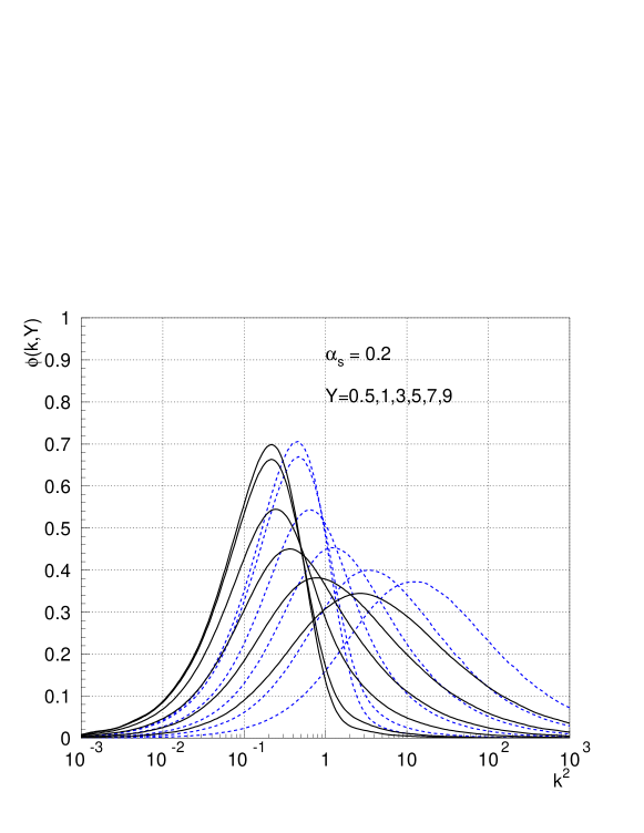
The change from the correlator of Wilson lines in the fundamental representation to the adjoint one corresponds to the emission of the gluon from the triple Pomeron vertex itself. This emission is not prohibited by the Abramovsky–Gribov–Kancheli (AGK) cutting rules [38] for inclusive gluon production in high energy QCD. It was argued previously [39, 40] that the numerical difference in the resulting rapidity distributions is rather small. In figure 1, we compare numerical solutions (to be discussed further shortly) for the unintegrated gluon distribution using the correlator of Wilson lines in the adjoint representation (eq. 15)) with the one using the correlator of Wilson lines in the fundamental representation (eq.16). The shape of the distribution is very similar, whereas the position of the peak is different. At $Y=0$ the position of the peaks differ by the ratio of the $C_{A}/C_{F}\simeq 2$. At higher values of $Y$ this difference increases due to the faster evolution of the correlator in the adjoint representation.

Figure 1: The unintegrated gluon distribution obtained from a) correlators in the adjoint representation (eq.15) (dashed lines) and b) correlators in the fundamental representation (eq. 16) (solid lines).

The BK equation is the simplest evolution equation capturing both the leading $\ln(1/x)$ BFKL dynamics at moderately small values of $x$, as well as the recombination physics of high parton densities at very small values of $x$. In the limit where the dipole scattering amplitude is small, $T\ll 1$, the non-linear term in eq. (9) can be ignored and the BK equation reduces to the BFKL equation. In this limit, the amplitude has the solution,

$$T(r_{\perp},Y) \approx (r_{\perp}^{2}Q_{0}^{2})^{1/2}\,e^{\omega{\overline{\alpha}_{s}}Y}\exp\left(-{\ln^{2}(1/r_{\perp}^{2}Q_{0}^{2})\over 2\beta{\overline{\alpha}_{s}}Y}\right)$$ (17)

$$= \exp\left({\rho\over 2}+\omega{\overline{\alpha}}_{s}Y-{\rho^{2}\over 2\beta{\overline{\alpha}}_{s}Y}\right)\;,$$

where $\omega=4\ln 2\approx 2.77$, $\beta=28\zeta(3)\approx 33.67$ and $\rho\equiv\ln(r_{\perp}^{2}Q_{0})^{2}$. If we define the saturation condition as

$$T(r_{\perp},Y)=\frac{1}{2}\quad\mbox{at\ \ }r_{\perp}={2\over Q_{s}}\;,$$ (18)

one gets [27]

$$Q_{s}^{2}=Q_{0}^{2}\,\,e^{c{\overline{\alpha}}_{s}Y}\quad\mbox{where}\;c\approx 4.84\;.$$ (19)

A more careful analysis of the BK-equation close to the saturation boundary gives solution $c\approx 4.88$. In the strong field (saturation) limit [25] where $T\approx 1$, one finds

$$T(r_{\perp},Y)=1-{\kappa}\;\exp\left(-{1\over 4c}\,\ln^{2}(r_{\perp}^{2}Q_{s}^{2})\right)\,,$$ (20)

with $c\approx 4.84$ and where $\kappa$ is an undetermined constant. In the large $Y$ asymptotic regime, leading and next-to-leading corrections to the form of the BK amplitude and the saturation scale have been computed [26, 28].

The coupling constant $\overline{\alpha}_{s}$ in eq. (9) is fixed in the leading logarithmic approximation in $1/x$. This leads to a rather strong dependence of the saturation scale in the leading logarithmic approximation: $Q_{s}\sim x^{-\lambda_{s}}$ with $\lambda_{s}\approx 4.88\,\bar{\alpha}_{s}$. For typical values of $\alpha_{s}$, of order $0.2$-$0.3$, $\lambda_{s}$ is at least a factor of three higher than fits to the HERA and RHIC data would suggest [48]. It is therefore desirable to include at least part of the next-to-leading corrections in $\ln(1/x)$ to the BK equation. Such corrections are known to reduce significantly the Pomeron intercept in the case of the BFKL equation.

The BK equation has been solved numerically for both fixed and running coupling [22, 23, 24, 42]. These solutions have the following features:

• The dipole amplitude is shown to unitarize, and the solution exhibits geometrical scaling.

• The saturation scale has the behavior in eq. (19) or $Q_{s}\sim\exp(\sqrt{\lambda\ln 1/x})$ in the fixed and running coupling cases respectively.

• The infrared diffusion problem of the BFKL solution is cured by the non-linear term in the BK equation.

• Ultraviolet diffusion is still present in the BK equation. However, it is attenuated by including running coupling effects [22, 42, 49].

In this work, we solved the BK equation numerically, in both fixed and running coupling cases, to investigate limiting fragmentation in hadronic collisions. In the fixed coupling case, since realistic values of $\alpha_{s}$ give too high a value of $\lambda_{s}$, we solved the BK equation with very small values of $\alpha_{s}$ chosen to give $\lambda_{s}$ values that are compatible with data from HERA, RHIC and hadron colliders. (We will see that these lower values are indeed favored by the data.) This is not unreasonable because it has been shown [28] that resummed next-to-leading order corrections to the BFKL equation in the presence of a unitary boundary (à la BK) give values of the saturation scale $\lambda_{s}$ that are nearly independent of the energy, as in the LO case, but with a much smaller value of $\lambda_{s}$.

The limited running coupling studies we performed did not give nearly as good agreement with the data than the fixed coupling studies with the lower values of $\alpha_{s}$. This is likely due to the fact that the energy dependence in this case is much too fast compared to the data. Further, since our results are sensitive to small transverse momenta, they will also depend strongly on how one regulates the running of $\alpha_{S}$ in the infrared. This requires a more detailed study than reported here. We shall therefore restrict ourselves to the fixed coupling case in discussing our results in the following section.

As explained before, the “unintegrated gluon distributions” $\phi_{{}_{A,B}}$ are obtained from solutions to eq. (9). At small values of $x$, where the gluon density is high, eq. (9) captures the essential physics of saturation; we therefore use it to determine $\phi(x,k_{\perp})$ for values of $x<x_{0}$ with $x_{0}=0.01$. For larger values of $x$ ($x\geq 0.01$), we used the phenomenological extrapolation,

$$\phi(x,k_{\perp})=\bigg{(}\frac{1-x}{1-x_{0}}\bigg{)}^{\beta}\,\bigg{(}\frac{x_{0}}{x}\bigg{)}^{\lambda_{0}}\,\phi(x_{0},k_{\perp})\;,\quad x>x_{0}\;.$$ (21)

The parameter $\beta=4$ is fixed by QCD counting rules [51]. We checked that the results are not sensitive to the variation of this parameter in the range $4-5$. The parameter $\lambda_{0}$ was varied between $0$ and $0.15$ in the fits to data discussed in the following section.

The initial condition for the BK evolution, that gives $\phi(x_{0},k_{\perp})$, is given by the McLerran-Venugopalan (MV) model [13] with a fixed initial value of the saturation scale $Q_{s}^{A}(x_{0})$. For a gold nucleus, extrapolations from HERA and estimates from fits to RHIC data suggest that $(Q_{s}^{A}(x_{0}))^{2}\approx 2\,{\rm GeV}^{2}$. The saturation scale in the proton is taken to be $Q_{s}^{2}(x_{0})=(Q_{s}^{A}(x_{0}))^{2}\,(197/A)^{1/3}$. For comparison, we also considered initial conditions from the Golec-Biernat and Wusthoff (GBW) model [48]. The values of $Q_{s}^{A}$ were varied in this study to obtain best fits to the data.

4 Results for Limiting Fragmentation

Experimental data are presented in terms of the measured distributions of produced charged hadrons. Our expression in eq. (5) is for produced gluons. Rapidity distributions are dominated by low $p_{\perp}$ ($p_{\perp}\leq Q_{s}$) particles; the detailed mechanism of how such soft gluons fragment to form hadrons is unknown. However, in $e^{+}e^{-}$ collisions, several studies have been performed of hadronization; it is observed that at scales comparable to $p_{\perp}\sim Q_{s}$, the distribution of produced hadrons mirrors that of the produced gluons. This hypothesis is known as “parton-hadron” duality [19] and we shall adopt it here. We will discuss the effect of fragmentation functions shortly.

Limiting fragmentation is often experimentally studied in terms of the measured pseudo-rapidity $\eta$ of produced particles. For massless particles, $\eta$ and $y$ are the same, but they differ for massive particles. One obtains

$$y(\eta,p_{\perp},m)\;=\;\frac{1}{2}\ln\left[\frac{\sqrt{m^{2}+p_{\perp}^{2}\,{\rm ch}^{2}\eta}+p_{\perp}\,{\rm sh}\eta}{\sqrt{m^{2}+p_{\perp}^{2}\,{\rm ch}^{2}\eta}-p_{\perp}\,{\rm sh}\eta}\right]\;.$$ (22)

We choose $m$ to be of order of $m\simeq 150\,{\rm MeV}-300\,{\rm MeV}$. Our expression for $dN/dy$ of gluons has a logarithmic divergence at low $p_{\perp}$; in addition to parton-hadron duality, for self consistency, we should regulate the corresponding expression for charged hadrons with the same mass as the one used in the conversion from $y$ to $\eta$. We will later discuss the sensitivity of our results to $m$.

We now have all the ingredients necessary to calculate the multiplicity distributions in the Color Glass Condensate framework. As discussed previously, experimental data on pseudo-rapidity distributions in the projectile fragmentation region scale with $\eta-Y_{\rm beam}$ for different energies. In eq. (5), $\phi_{{}_{A}}(x_{1})$ depends on the difference $y-Y_{\rm beam}$ and $\phi_{{}_{B}}(x_{2})$ on the sum $y+Y_{\rm beam}$. To provide a sense of the $x$’s involved, consider gold-gold collisions at RHIC. For $y=Y_{\rm beam}$, which lies in the fragmentation region, and $p_{\perp}\sim m_{N}\sim 1$ GeV , $x_{1}\approx 1$ and $x_{2}\approx 2.5\cdot 10^{-5}$. One is therefore probing very small values of $x_{2}$ in nuclei in this region, where the saturation scale $Q_{s}(x_{2})$ is rather large. As we discussed previously, in this kinematic region, because of unitarity, the gluon distribution depends only weakly on $x_{2}\sim\exp(-(y+Y_{\rm beam}))$. This qualitatively explains the scaling in the limiting fragmentation region.

We now turn to our results. To reiterate, they are obtained by a) solving the BK equation to obtain eq. (11), and thereby eq. (15) for the unintegrated distribution for $x\leq 10^{-2}$, b) using eq. (21) to determine the large $x$ ($x\geq 10^{-2}$) behavior, and c) substituting these in eq. (5) to determine rapidity distribution of gluons. The pseudo-rapidity distributions are determined by the transformation in eq. (22).

Figure 2: Pseudorapidity distributions $dN/d\eta$ for charged particles from nucleon-nucleon collisions at UA5 energies [5] $\sqrt{s}=53,200,546,900\,{\rm GeV}$ and PHOBOS data [8] at $\sqrt{s}=200\,{\rm GeV}$. Upper plots: initial distribution from the MV model, lower plots: initial distribution from the GBW model. Left panels: $\lambda_{0}=0.15$, right panels $\lambda_{0}=0.0$.

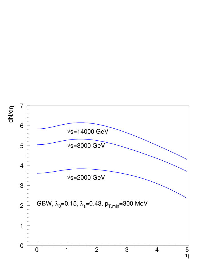
In figure 2 we show pseudo-rapidity distributions of the charged particles produced in nucleon-nucleon collisions for center of mass energies ranging from $53\,{\rm GeV}$ to $900\,{\rm GeV}$. We have performed calculations for two different input distributions at starting value of $x_{0}=0.01$, namely, the GBW and MV models. The normalization has been treated as a free parameter. Extrapolations to large values of $x$ are performed using the formula in eq. (21). Plots on the left hand side of figure 2 are obtained for $\lambda_{0}=0.15$ whereas the right hand side plots are done for $\lambda_{0}=0.0$. The different values of $\lambda_{s}$ are obtained by varying $\alpha_{s}$ when solving the BK equation.

Note that while $\lambda_{s}$ controls the growth of $Q_{s}$ with energy, the amplitude in eq. (17) has the growth rate

$$\lambda_{\rm BK}=\frac{2.77}{4.88}\,\lambda_{s}\approx 0.57\,\lambda_{s}\,,$$

which is significantly lower. So $\lambda_{s}=0.46$, which gives reasonable fits (more on this in the next paragraph) to the pp data for the MV initial conditions, corresponds to $\lambda_{\rm BK}=0.28$, which is close to the value for the energy dependence of the amplitude in next-to-leading order resummed BK computations [28] and in empirical dipole model comparisons to the HERA data [48].

We find that our computations are extremely sensitive to the extrapolation prescription to large $x$. This is not a surprise since we are probing the wave-function of the projectile at fairly large values of $x_{1}$. From our analysis, we see that the data naively favor a non-zero value for $\lambda_{0}$ in eq. (21). The zero value of $\lambda_{0}$ results in the distributions which, in both the MV and GBW cases give reasonable fits (albeit with different normalizations) at lower energies but systematically become harder relative to the data as the energy is increased. To fit the data in the MV model up to the highest UA5 energies, a lower value of $\lambda_{s}$ than that in the GBW model is required. This is connected with the fact that MV model has tails which extend to larger values in $k_{\perp}$ than in the GBW model. As the energy is increased, the typical $k_{\perp}\sim Q_{s}(x_{2})$ does as well. We will return to this point shortly.

Figure 3: The same as figure 2 but plotted versus $\eta^{\prime}=\eta-Y_{\rm beam}$ to illustrate the region of limiting fragmentation.

In figure 3 the same distributions are shown as a function of the $\eta^{\prime}=\eta-Y_{\rm beam}$. The calculations for $\lambda_{0}=0.15$, are consistent with scaling in the limiting fragmentation region. There is a slight discrepancy between the calculations and the data in the mid-rapidity region. This discrepancy may be a hint that one is seeing violations of $k_{\perp}$ formalism in that regime because $k_{\perp}$ formalism becomes less reliable the further one is from the dilute-dense kinematics of the fragmentation regions [37, 36]. This discrepancy should grow with increasing energy. However, our parameters are not sufficiently constrained that a conclusive statement can be made.

In changing from rapidity to pseudo-rapidity distributions, one has to use a Jacobian with a mass parameter. We have chosen this parameter, for consistency, to be the same as our $p_{\perp}$ cut-off for the integration over the transverse momentum in the formula for the gluon production. We have checked the sensitivity of our calculations to variations in the $p_{\perp}$ cut-off $m$ in the range $150-300\,{\rm MeV}$. In figure 4 we show the results for the pp collisions with two different values of $p_{\perp,{\rm min.}}\;=\;150,300\,{\rm GeV}$. The ‘dip’ in the pseudo-rapidity distribution becomes more or less pronounced when the parameter $m$ is decreased or increased respectively. We note that in order to obtain a reasonable description of the data we also had to adjust the other parameters (normalization and $\lambda_{s}$).

Figure 4: Calculations for different values of the infrared $p_{T}$ cutoff compared to the pp data in figure 2.

In figure 5 we show the extrapolation to higher energies, in particular the LHC range of energies for the calculation with the GBW input. We observed previously that the MV initial distribution, when evolved to these higher energies, gives a rapidity distribution which is very flat in the $-5<\eta<5$ regime. We noted that this is because the average transverse momentum grows with the energy giving a significant contribution from the high $k_{\perp}$ tail of the distribution in the MV input in eq. (21).

The effect of fragmentation functions on softening the spectra in the limiting fragmentation region can be simply understood by the following qualitative argument. The inclusive hadron distribution can be expressed as

$$\frac{dN_{h}}{d^{2}p_{\perp}dy}=\int_{z_{\rm min.}}^{1}\frac{dz}{z}\,\frac{dN_{g}}{d^{2}q_{\perp}dy}\,D_{g\rightarrow h}\left(z=\frac{p_{\perp}}{q_{\perp}},\mu^{2}\right)\,,$$ (23)

where $D_{g\rightarrow h}(z,\mu^{2})$ is the fragmentation function denoting the probability, at the scale $\mu^{2}$, that a gluon fragment into a hadron carrying a fraction $z$ of its transverse momentum. For simplicity, we only consider here the probability for gluons fragmenting into the hadron. The lower limit of the integral can be determined from the kinematic requirement that $x_{1,2}\leq 1$–we obtain,

$$z_{\rm min.}=\frac{q_{\perp}}{m_{N}}\,e^{y-Y_{\rm beam}}\,.$$ (24)

if $z_{\rm min.}$ were zero, the effect of including fragmentation effects would simply be to multiply eq. (23) by an overall constant factor. At lower energies, the typical value of $q_{\perp}$ is small for a fixed $y-Y_{\rm beam}$; the value of $z_{\rm min.}$ is quite low. However, as the center of mass energy is increased, the typical $q_{\perp}$ value grows slowly with the energy. This has the effect of raising $z_{\rm min.}$ for a fixed $y-Y_{\rm beam}$, thereby lowering the value of the multiplicity in eq.(23) for that $y-Y_{\rm beam}$. Note further that eq. (24) suggests that there is a kinematic bound on $q_{\perp}$ as a function of $y-Y_{\rm beam}$–only very soft gluons can contribute to the inclusive multiplicity.

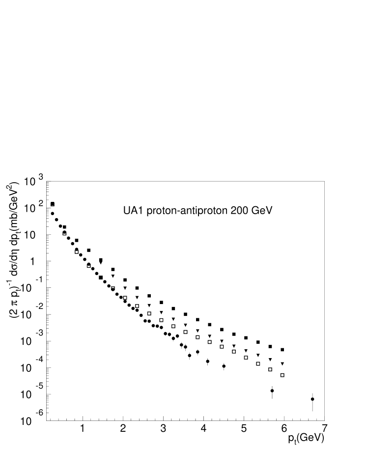
In figure 6 we illustrate $p_{\perp}$ distributions obtained from the MV input compare to the UA1 data [52]. We compare the calculation with and without the fragmentation function. The fragmentation function has been taken from [53]. Clearly the “bare” MV model does not describe the data at large $k_{\perp}$ because it does not include fragmentation function effects which, as discussed, make the spectrum less flat. In contrast, because the $k_{\perp}$ spectrum of the GBW model dies exponentially at large $k_{\perp}$, this “unphysical” $k_{\perp}$ behavior mimics the effect of fragmentation functions–see figure 6. Hence extrapolations of this model, as shown in figure 5 give a more reasonable looking result. Similar conclusions were reached previously in Ref. [44].

Figure 5: Predictions for higher center-of-mass energies: $\sqrt{s}=2,8,14\,{\rm TeV}$ for GBW input model. Parameter in the large $x$ extrapolation was set to $\lambda_{0}=0.15$.

Figure 6: $p_{\perp}$ distribution from eq. (5) with MV (full squares) and GBW (full triangles) initial conditions. The MV initial condition–with the fragmentation function included–is denoted by the open squares. The distribution is averaged over the rapidity region $y=0.0-2.5$, to compare with data (in 200 GeV/nucleon proton-antiproton collisions in the same pseudo-rapidity range) on charged hadron $p_{\perp}$ distributions from the UA1 collaboration: full circles.

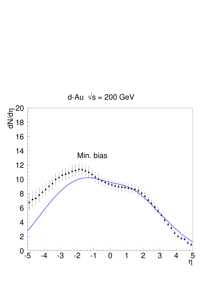
We next compute the pseudo-rapidity distribution in deuteron-gold collisions. In figure 7 we show the result for the calculation compared with the dA data [8]. The unintegrated gluons were extracted from the pp and AA data. The overall shape of the distribution matches well on the deuteron side with the minimum-bias data. The disagreement on the nuclear fragmentation side is easy to understand since, as mentioned earlier, it requires a better implementation of nuclear geometry effects. Similar conclusions were reached in Ref. [31] in their comparisons to the RHIC deuteron-gold data.

Figure 7: Comparison of computations to minimum bias deuteron-gold data at RHIC [8]. Calculation done using the MV model as a starting distribution for the evolution.

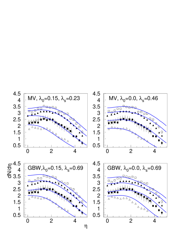
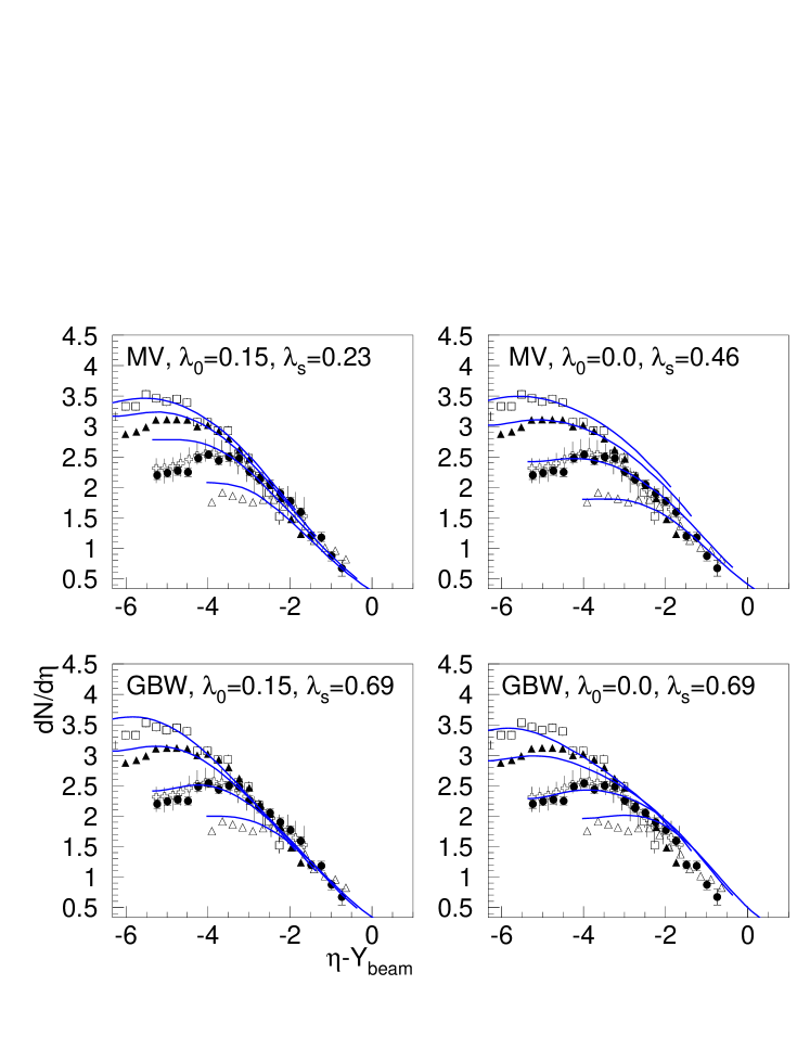
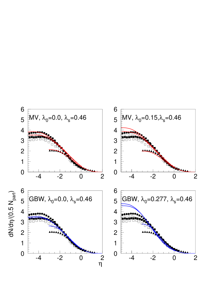
We now apply our considerations to central nucleus–nucleus collisions. In figure 8 we present fits to data on the pseudo-rapidity distributions in gold–gold collisions from the PHOBOS, BRAHMS and STAR collaborations. The data [8] are for $\sqrt{s}=19.6,130,200\,{\rm GeV}$ and the BRAHMS data [7] are for $\sqrt{s}=130,200\,{\rm GeV}$. A reasonable description of limiting fragmentation is achieved in this case as well. One again has discrepancies in the central rapidity region as in the pp case. As mentioned previously, a natural explanation for this discrepancy is the violation of $k_{\perp}$-factorization. It is expected that these violations decrease the multiplicity in this regime [37, 36] relative to extrapolations using $k_{\perp}$-factorization. We find that values of $Q_{s}^{A}\approx 1.3$ GeV for the saturation scale give the best fits. This value is consistent with other estimates [37, 30, 33]. Apparently the gold-gold data are better described by the calculations which have $\lambda_{0}=0.0$. This might be related to the difference in the large $x$ distributions in the proton and nucleus. Also, slightly higher values of $\lambda_{s}$ are preferred. This variation of parameters from AA to pp case might be also connected with the fact that in our approach the impact parameter is integrated out, so that there is no detailed information on the nuclear geometry. A more detailed calculation with the impact parameter dependence taken into account is left for future investigations.

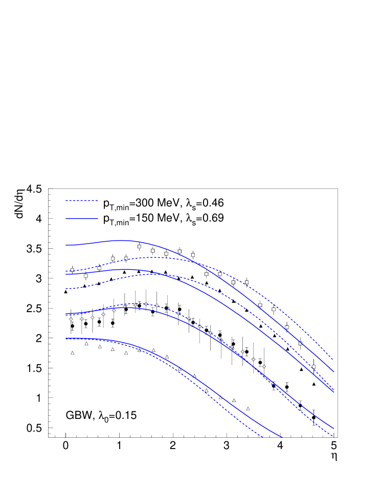
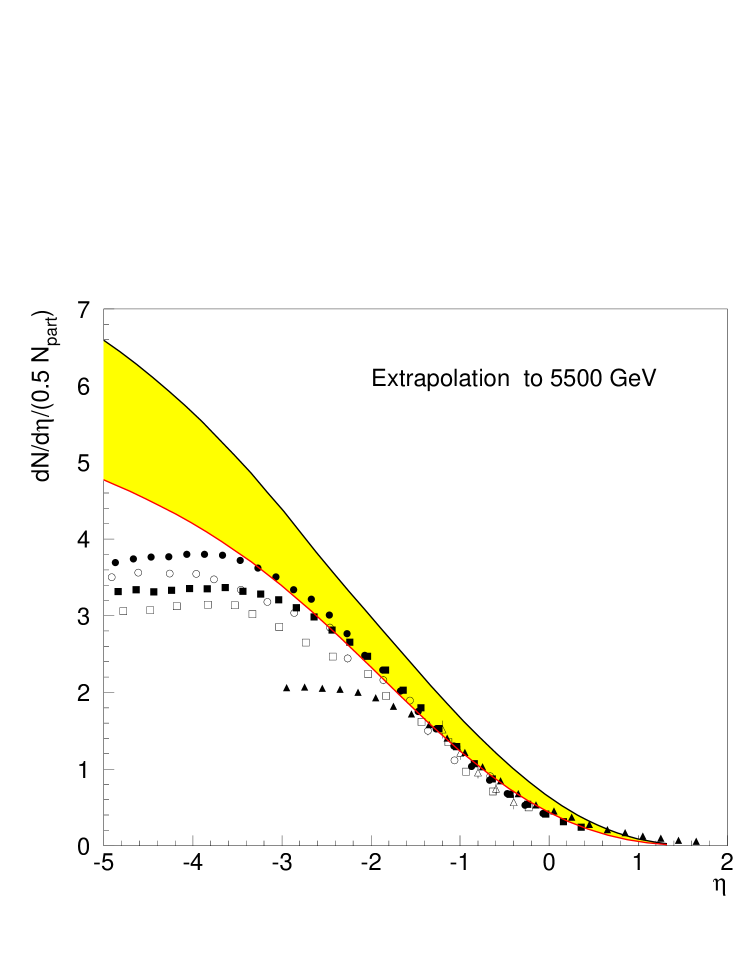
In fig. 9 we show the extrapolation of two calculations to higher energy $\sqrt{s}=5500\;{\rm GeV}$. We note that the calculation within the MV model gives results which would violate the scaling in the limiting fragmentation region by approximately $25\%$ at larger $y-Y_{\rm beam}$. This violation is partly because of the effect of fragmentation functions discussed previously and in part due to the fact that the integrated parton distributions from the MV model do not obey Bjorken scaling at large values of $x$. In the latter case, the violations are proportional to $\ln(Q_{s}^{2}(x_{2}))$ as discussed previously. The effects of the former are simulated by the GBW model-the extrapolation of which, to higher energies, is shown by the dashed line. The band separating the two therefore suggests the systematic uncertainity in such an extrapolation coming from a) the choice of initial conditions and b) the effects of fragmentation functions which are also uncertain at lower transverse momenta.

Finally, the transverse momentum distribution in the gold-gold collisions is presented in fig. 10. The data at $\sqrt{s}=200{\rm GeV}$ are from the PHOBOS collaboration [11]. Again, in this case, the calculation without fragmentation function tends to overshoot the data significantly at high values of $p_{t}$. Including fragmentation function effects [53] results in a better agreement with the shape of the $p_{t}$ distribution as expected. A more detailed study to extract parameters that give the best chi-squared values will be performed at a later date.

Figure 8: Pseudorapidity distributions normalized by the number of participants for charged hadrons in gold-gold collisions from the PHOBOS collaboration at energies $19.6,130,200\,{\rm GeV}$ (filled triangles , squares and circles), BRAHMS collaboration at energies $130,200\,{\rm GeV}$ (open squares and circles) . The data from the STAR collaboration at energy $62.4\,{\rm GeV}$ (open triangles) are not visible on this plot but can be seen more clearly in fig. 9. Upper plots: initial distributions from the MV model; lower plots: initial distributions from the GBW model.

Figure 9: Extrapolation of calculations for gold-gold collisions shown in fig. 8 to the LHC energy $\sqrt{s}=5500\;{\rm GeV}$/ nucleon. For comparison, the same data at lower energies are shown. (See fig. 8.) The band is an estimate of the systematic uncertainty of our approach. Its lower border corresponds to the GBW input with $\lambda_{0}=0,\lambda_{s}=0.46$, and its upper border to the MV input with $\lambda_{0}=0,\lambda_{s}=0.46$.

Figure 10: $p_{\perp}$ distribution from eq. (5) with MV (full triangles) initial conditions. The MV initial condition with the fragmentation function included is denoted by the full squares. The distribution is averaged over the pseudo-rapidity region $y=0.2-1.4$, to compare with data in 200 GeV/nucleon gold-gold collisions (open circles).

5 Conclusions

We studied here the phenomenon of limiting fragmentation in the Color Glass Condensate framework. In the dilute-dense (projectile-target) kinematics of the fragmentation regions, one can derive (in this framework) an expression for inclusive gluon distributions which is $k_{\perp}$ factorizable into the product of “unintegrated” gluon distributions in the projectile and target. From the general formula for gluon production(eq. (5)), limiting fragmentation is a consequence of two factors:

• Unitarity of the $U$ matrices which appear in the definition of the unintegrated gluon distribution in eq. (6).

• Bjorken scaling at large $x_{1}$, namely, the fact that the integrated gluon distribution at large $x$, depends only on $x_{1}$ and not on the scale $Q_{s}(x_{2})$. (The residual scale dependence consequently leads to the dependence on the total center-of-mass energy.)

Deviations from the limiting curve at experimentally accessible energies are very interesting because they can potentially teach us about how parton distributions evolve at high energies. In the CGC framework, the Balitsky–Kovchegov equation determines the evolution of the unintegrated parton distributions with energy from an initial scale in $x$ chosen to be $x_{0}=0.01$. This choice of scale is inspired by model comparisons to the HERA data.

We compared our results to data on limiting fragmentation from pp collisions at various experimental facilities over a wide range of collider energies, and to collider data from RHIC for deuteron-gold and gold-gold collisions. We obtained results for two different models of initial conditions at $x\geq x_{0}$; the McLerran-Venugopalan model (MV) and the Golec-Biernat–Wusthoff (GBW) model. In addition to the two parameters in the initial conditions ($\lambda_{s}$ and $\lambda_{0}$), we also studied the sensitivity of our results to an infrared momentum cut-off $m$ (chosen to be the same value in the $y\rightarrow\eta$ conversion for hadrons).

We found reasonable agreement for this wide range of collider data for the limited set of parameters. Clearly these can be fine tuned by introducing further details about nuclear geometry. That would introduce further parameters but on the other hand there is more data for different centrality cuts as well-we leave these detailed comparisons for future studies. In addition, an important effect, which improves agreement with data, is to account for the fragmentation of gluons in hadrons. In particular, the MV model, which has the right leading order large $k_{\perp}$ behavior, but no fragmentation effects, is much harder than the data. The latter falls as a much higher power of $k_{\perp}$. Since even rapidity distributions at higher energies data are more sensitive to larger $k_{\perp}$, we expect this discrepancy to show up in our studies of limiting fragmentation and indeed it does. We noticed that taking this into account lead to much more plausible extrapolations of fits of existing data to LHC energies. This “gluon fragmentation” contribution also suggests that the “flat” deviations that we found (for fits with MV initial conditions) for $\lambda_{s}=0.46$ ($\lambda_{\rm BK}=0.28$) are diminished.

Clearly, the procedure employed in this paper needs further improvements. One of them is the impact parameter dependence of the unintegrated gluon distribution functions. We discussed briefly “gluon fragmentation” effects (with different fragmentation function sets) which need to be taken into account. Furthermore, large $x$ distributions also need to be better constrained and consistency with computations of other final states in the CGC framework established. Finally, the factorization formula used in this paper involves only gluons; for more realistic estimates, one should also include quark distributions in this framework.

References

- [1] J. Benecke, T.T. Chou, C.N. Yang and E. Yen, Phys. Rev. 188 (1969) 2159.
- [2] A. Donnachie and P.V. Landshoff, Phys. Lett. B296 (1992) 227.
- [3] M.M. Block and F. Halzen, Phys. Rev. D70 (2004) 091901; Phys. Rev. D72 (2005) 036006, Erratum-ibid. D72 (2005) 039902.
- [4] V. Berardi et al., TOTEM coll., CERN-LHCC-2004-002.
- [5] G.J Alner et al, Z. Phys. C33 (1986) 1.
- [6] J.E. Elias et al, Phys. Rev. D 22 (1980) 13.
- [7] I.G. Bearden et al, BRAHMS coll., Phys. Lett. B 523 (2001) 227; Phys. Rev. Lett. 88 (2002) 20230.
- [8] B.B. Back et al, PHOBOS coll., Phys. Rev. Lett., 91, (2003), 052303; nucl-ex/0509034.
- [9] J. Adams et al, STAR coll., Phys. Rev. Lett. 95 (2005) 062301; Phys. Rev. C73 (2006) 034906.
- [10] B.B. Back et al, PHOBOS coll., Phys. Rev. C70, (2004) 061901(R) .
- [11] B.Back et al, PHOBOS coll., Phys. Lett. B578 (2004) 297.
- [12] J. Jalilian-Marian, Phys. Rev. C 70 (2004) 027902.
- [13] L.D. McLerran and R. Venugopalan, Phys. Rev. D49 (1994) 2233; Phys. Rev. D49 (1994) 3352; Phys. Rev. D50 (1994) 2225.
- [14] For a review of the CGC, see: E. Iancu and R. Venugopalan, hep-ph/0303204.
- [15] J. Jalilian-Marian, A. Kovner, L.D. McLerran and H. Weigert, Phys. Rev. D55: 5414 (1997); J. Jalilian-Marian, A. Kovner, A. Leonidov and H. Weigert, Nucl. Phys. B 504 (1997) 415; Phys. Rev. D 59 (1999) 014014; J. Jalilian-Marian, A. Kovner and H. Weigert, Phys. Rev. D 59 (1999) 014015; E. Iancu, A. Leonidov and L.D. McLerran, Nucl.Phys. A692 (2001) 583; E. Ferreiro, E. Iancu, A. Leonidov and L.D. McLerran, Nucl. Phys. A 703, 489 (2002); E. Iancu, A. Leonidov and L. D. McLerran, Phys. Lett. B510, 145 (2001).
- [16] I. I. Balitsky, Nucl. Phys. B463 (1996) 99; Phys. Rev. Lett. 81 (1998) 2024; Phys. Rev. D60 (1999) 014020; Phys. Lett. B518 (2001) 235.
- [17] Yu. V. Kovchegov, Phys. Rev. D60 (1999) 034008; Phys. Rev. D 61, 074018 (2000).
- [18] A.H. Mueller, hep-ph/0111244, CU-TH-1035.
- [19] Y.L. Dokshitzer, V.A. Khoze, A.H. Mueller and S.I. Troian, Basics of perturbative QCD, Ed. Frontières, Gif-sur-Yvette, France, p274 (1991).
- [20] J. Jalilian-Marian and Y. V. Kovchegov, Prog. Part. Nucl. Phys. 56, 104 (2006).
-
[21]
L. N. Lipatov, Sov. J. Nucl. Phys.
23 (1976) 338;
E. A. Kuraev, L. N. Lipatov and V. S. Fadin, Sov. Phys. JETP 45 (1977) 199;
I. I. Balitsky and L. N. Lipatov, Sov. J. Nucl. Phys. 28 (1978) 338. -
[22]
M. A. Braun, Eur. Phys. J. C16 (2000) 337; hep-ph/0010041;
N. Armesto and M. A. Braun, Eur. Phys. J. C20 (2001) 517. - [23] E. Gotsman, E.M. Levin, M. Lublinsky and U. Maor, Nucl. Phys. A 696 (2001) 851; E. Gotsman, E.M. Levin, M. Lublinsky and U. Maor, Eur. Phys. J. C27 (2003) 411; E. Levin and M. Lublinsky, Nucl. Phys. A696 (2001) 833; M. Lublinsky, Eur. Phys. J. C21 (2001) 513.
- [24] K. Golec-Biernat, L. Motyka and A.M. Staśto, Phys. Rev. D65 (2002) 074037.
- [25] E. Levin and K. Tuchin, Nucl. Phys. A691, 779 (2001); E. Iancu, A. Leonidov and L. D. McLerran, Phys. Lett. B510, 133 (2001).
- [26] S. Munier and R. Peschanski, Phys. Rev. D69 (2004) 034008.
- [27] A.H. Mueller and D. Triantafyllopoulos, Nucl. Phys. B640 (2002) 331.
- [28] D. N. Triantafyllopoulos, Nucl. Phys. B648, 293 (2003); Acta Phys. Polon. B36, 3593 (2005).
- [29] L.V. Gribov, E.M. Levin and M.G. Ryskin, Phys. Rept. 100 (1983) 1.
- [30] D. Kharzeev and E. Levin, Phys. Lett. B523 (2001) 79;
- [31] D. Kharzeev, E. Levin and M. Nardi, Phys. Rev. C71 (2005) 054903; Nucl. Phys. A730 (2004) 448, Erratum-ibid. A743 (2004) 329; Nucl. Phys. A747 (2005) 609.
- [32] A. Dumitru, L. Gerland and M. Strikman, Phys. Rev. Lett. 90, 092301 (2003); [Erratum-ibid. 91, 259901 (2003)]
- [33] H. Kowalski and D. Teaney, Phys. Rev. D68, 114005 (2003).
- [34] Y.V. Kovchegov and K. Tuchin, Phys. Rev. D65 (2002) 074026.
- [35] D. Kharzeev, Y. V. Kovchegov and K. Tuchin, Phys. Rev. D68, 094013 (2003).
- [36] I. Balitsky, Phys. Rev. D72, 074027 (2005).
- [37] A. Krasnitz, Y. Nara and R. Venugopalan, Phys. Rev. Lett. 87, 192302 (2001); Nucl. Phys. A717, 268 (2003); Nucl. Phys. A727, 427 (2003).
- [38] V. A. Abramovsky, V. N. Gribov and O. V. Kancheli, Yad. Fiz. 18, 595 (1973) [Sov. J. Nucl. Phys., 18, 308 (1974)].
- [39] M.A. Braun, Phys. Lett. B599 (2004) 269.
- [40] M.A. Braun, Eur. Phys. J. C42 (1995) 169, hep-ph/0502184.
- [41] M.A. Braun, Phys. Lett. B576 (2003) 115.
- [42] K. Rummukainen and H. Weigert, Nucl. Phys. A739 (2004) 183.
[43]
M. Hirai, S. Kumano and M. Miyama, Phys. Rev. D64 (2001) 034003;
M. Hirai, S. Kumano and T.-H. Nagai, Phys. Rev. C70 (2004) 044905. K. J. Eskola, V. Kolhinen and C. Salgado, Eur. Phys. J. C9 (1999) 61, D. De Florian and Sassot, Phys. Rev. D69 (2004) 074028. - [44] A. Szczurek, Acta Phys. Polon. B34 (2003) 3191.
- [45] J.-P. Blaizot, F. Gelis and R. Venugopalan, Nucl. Phys. A743 (2004) 13.
- [46] J. P. Blaizot, F. Gelis and R. Venugopalan, Nucl. Phys. A743 (2004) 57.
- [47] A. Bialas and M. Jeżabek, Phys. Lett. B590 (2004) 233.
- [48] K. Golec-Biernat and M. Wusthoff, Phys. Rev. D59 (1999) 014017.
- [49] J.L. Albacete, N. Armesto, J.G. Milhano, C.A. Salgado and U.A. Wiedemann, Phys. Rev. D71 (2005) 014003.
- [50] H. Fujii, F. Gelis and R. Venugopalan, hep-ph/0603099; Phys. Rev. Lett. 95 (2005) 162002.
- [51] S. J. Brodsky and G. R. Farrar, Phys. Rev. D11, 1309 (1975); V. A. Matveev, R. M. Muradian and A. N. Tavkhelidze, Lett. Nuovo Cim. 7, 719 (1973).
- [52] C. Albajar et al., UA1 coll., Nucl. Phys. B335 (1990) 261.
- [53] B.A. Kniehl, G. Kramer and B. Potter, Nucl. Phys. B582 (2000) 514.