Production of black holes and their angular momentum distribution in models with split fermions

Abstract

In models with TeV-scale gravity it is expected that mini black holes will be produced in near-future accelerators. On the other hand, TeV-scale gravity is plagued with many problems like fast proton decay, unacceptably large $n-{\bar{n}}$ oscillations, flavor changing neutral currents, large mixing between leptons, etc.. Most of these problems can be solved if different fermions are localized at different points in the extra dimensions. We study the cross-section for the production of black holes and their angular momentum distribution in these models with “split” fermions. We find that, for a fixed value of the fundamental mass scale, the total production cross section is reduced compared with models where all the fermions are localized at the same point in the extra dimensions. Fermion splitting also implies that the bulk component of the black hole angular momentum must be taken into account in studies of the black hole decay via Hawking radiation.

I Introduction

There are relatively few robust experimental predictions of quantum gravity. One of those few is that particle collisions with center-of-mass energies sufficiently greater than the fundamental scale of quantum gravity, whatever that may be, should result in the formation of black holes. Unfortunately, in traditional models of quantum gravity the fundamental scale of gravity is the Planck scale, $M_{Pl}\simeq 1.5\times 10^{19}$GeV – an energy scale well beyond the reach of both particle accelerators and (because of the rapid decrease in cosmic ray flux with increasing energy) cosmic ray detectors. However, over the last decade considerable attention has focused on models in which the fundamental quantum gravity energy scale $M_{\star}\mathrel{\raise 1.29167pt\hbox{$>$}\mkern-14.0mu\lower 2.58334pt\hbox{$\sim$}}1$TeV ADD . In these models, the weakness of gravity is due to the existence of extra dimensions with large volume, $V^{(d)}$, in fundamental units $\ell_{\star}^{d}\equiv(1/M_{\star})^{d}$. (Here $d$ is the number of extra dimensions.)

The characteristic size of the extra dimensions can be as large as $0.2$mm (although it is generally much smaller). This leaves a lot of room for classical description of higher dimensional objects, eg. higher dimensional black holes. If two incoming particles collide with a center-of-mass (COM) energy $E_{CM}$ that is greater than $M_{*}$, and an impact parameter smaller than the gravitational radius (Schwarzschild radius for a static or outermost horizon radius for a rotating black hole) corresponding to $E_{CM}$, then one expect a black hole of mass $M_{bh}\mathrel{\raise 1.29167pt\hbox{$<$}\mkern-14.0mu\lower 2.58334pt\hbox{$\sim$}}E_{CM}$ will form. The exciting possibility is that such black holes might be produced and studied in near-future accelerator experiments BHacc . For example, the Large Hadron Collider (LHC), due to start operating in $2007$, will have $E_{CM}\simeq 14$TeV. Numerical estimates BHacc have suggested that it should produce ${\cal O}(10^{7})$ black holes per year if $M_{\star}\mathrel{\raise 1.29167pt\hbox{$<$}\mkern-14.0mu\lower 2.58334pt\hbox{$\sim$}}1$TeV. Black holes might also be produced by ultra-high energy cosmic rays scattering off nucleons in the Earth’s atmosphere fs and be observed using new detectors like the Auger observatory (however see ssd ).

Low scale quantum gravity certainly offers a rich opportunity for higher dimensional phenomenology. However, if one is concerned about realistic predictions for actual accelerator processes (eg. black hole production at the LHC), one must worry about a host of unacceptable predictions of low scale quantum gravity models problems . Low scale gravity is plagued with many problems like fast proton decay, unacceptably large $n\bar{n}$ oscillations, flavor changing neutral currents, large mixing between leptons, etc..

One solution to at least some of these problems is to gauge baryon (B) and lepton (L) number. However, gauging B or L has proven to be problematic. If $U(1)_{B}$ were an unbroken gauge symmetry, there would be a long range interaction not seen in experiments. Therefore, $U(1)_{B}$ needs to be broken down to a discrete gauge symmetry. The leftover discrete symmetry could preserve baryon number modulo some integer KraussWilczek . To suppress dangerous $n\rightarrow\bar{n}$ (neutron-antineutron) oscillations one must forbid both $\Delta B=1$ and $2$ operators. The allowed operators of lowest dimension would then be $\Delta B\geq 3$, and would be of dimension $12$ and higher. The most common problem in building models with gauged baryon number is arranging for the cancellation of gauge anomalies IbanezRoss . This requires either an unusual charge assignment to existing particles or the introduction of new exotic particles. There are other problems related to the idea of gauge coupling unification. The same statements are true for $U(1)_{L}$ as an unbroken gauge symmetry. It is therefore convenient to search for alternative solutions to the problems of TeV scale gravity.

A widely studied alternative to gauging baryon or lepton number in order to protect the proton is the so called “split fermion” model ArkaniHamedetal . In this model, standard model fields are confined to a “thick” brane – much thicker than $M_{\star}^{-1}$. Quarks and leptons are stuck on different three-dimensional slices within the thick brane (or on different branes), separated by much more than $M_{\star}^{-1}$. This separation causes an exponential suppression of all direct quantum-gravity couplings (of the type QQQL) between quarks and leptons, by resulting in exponentially small wave functions overlaps. If the spatial separation between the quarks and leptons is greater by a factor of at least 10 than the widths of their wave functions, then the proton decay rate will be safely suppressed.

The splitting of leptons from quarks does not suppress $\Delta B=2$ processes, like $n-{\bar{n}}$ oscillations, which are mediated by operators of the type uddudd. That requires, for example, further splitting between up-type and down-type quarks. Since the experimental limits on $\Delta B=2$ operators are much less stringent than those on $\Delta B=1$ operators, it is enough that the u and d quarks be separated by a factor of several times the width of their wave functions.

Splitting between the different quark flavors may have some unexpected advantages. Namely, one can explain Yukawa coupling hierarchy by introducing quark “geography” in extra dimensions geog . Presumably, the Higgs field, H, propagates freely between the sheets (branes) where quarks, Q, are localized. Different separations between different quark flavors results in different wave function overlaps for operators of the type HQQ involving those flavors, and thus different effective four-dimensional Yukawa couplings.

The need to suppress both flavor changing neutral currents and mixing between the neutrino generations requires further splitting between the different lepton flavors and generations. Finally, there is a problem of unacceptably large left-handed Majorana neutrino masses. This cannot be solved by splitting but requires some other fix. However, the purpose of this paper is to discuss black hole phenomenology at the LHC and our discussion is not much affected by the details of lepton location in extra dimensions. We therefore assume that the black hole phenomenology will be unaffected by the particular solution to the neutrino left-handed Majorana mass problem.

At low energies that do not probe the separation between the fermions, we must recover the standard ($3+1$)-dimensional results. These energies are not interesting for black hole production at the LHC. However, at energies and momentum transfers high enough to produce black holes, one will probe the fermion separations. One therefore expects that the “standard” ($3+1$)-dimensional black hole production cross section and angular momentum distribution will be significantly modified.

After a black hole is formed (eg. at the LHC), it decays by emitting Hawking radiation with temperature $T\sim 1/r_{h}$, where $r_{h}$ is the horizon radius of the black hole. Thermal Hawking radiation consists of two parts: (1) particles propagating along the brane, and (2) bulk radiation. The bulk radiation includes bulk gravitons. The bulk radiation is usually neglected. The justification is as follows. The wavelength of emitted radiation is larger than the size of the black hole, so the black hole behaves as a point radiator, radiating mostly in s-wave. Thus, the radiation for each particle mode will be equally probable in every direction (brane or bulk). For each particle that can propagate in the bulk there is a whole tower of bulk Kaluza-Klein excitations, but, since each excitation is only weakly coupled (due to small wave function overlap) to the small black hole, the whole tower counts only as one particle. Since the total number of species that are living on the brane is quite large ( $\sim 60$) while there is only one graviton, radiation along the brane should be dominant (see eg. EHM ).

This reasoning works very well if the black hole is not rotating. Rotation can significantly modify this conclusion. For high energy scattering of two particles with a non-zero impact parameter, the formation of a rotating black hole is much more probable than the formation of a non-rotating black hole. One expects that mainly highly rotating mini black holes will be formed in such scattering.

The number of graviton degrees of freedom in $(n+1)$-dimensional space-time is $N=(n+1)(n-2)/2$, which is just the number of possible polarizations of a spin 2 particle in an $n$-dimensional space. For example, for $n+1=10$ we have $N=35$. If a black hole is non-rotating, we expect emission of particles with non-zero spin (eg. gravitons) to be suppressed with respect to emission of scalar quanta as happens in $(3+1)$-dimensional space-time Page:76 (see also Section 10.5 FrNo and references therein). However, rotating black holes exhibit the phenomenon of super-radiance. Due to the existence of an ergosphere (a region between the infinite redshift surface and the event horizon), some of the modes of radiation get amplified, taking away the rotational energy of the black hole. Super-radiance is strongly spin-dependent, and emission of higher spin particles is strongly favored. For an extremal rotating black hole, the emission of gravitons is a dominant effect. For example, $(3+1)$-dimensional numerical calculations done by Page Page:76 (see also FrNo ) show that the probability of emission of a graviton by an extremal rotating black hole is about 100 times higher than the probability of emission of a photon or neutrino. In Kerr5D , it was shown that super-radiance also exists in higher dimensional space-times. Mini black holes created in high energy scattering are expected to have high angular momentum. We therefore expect a much higher proportion of the initial black hole mass to be dissipated as bulk gravitons.

It is known that in the highly non-linear, time-dependent and violent process of black hole creation, much of the initial center of mass energy is lost to gravitational radiation. This is up to 30% in $3+1$ dimensions, and may be larger in higher dimensions, due to the larger number of gravitational degrees of freedom. Since gravitons are not bound to the brane, most of them would be radiated in the bulk. Bulk graviton radiation may well dominate over the radiation of other particles in the brane, at least in the first stages of black hole evaporation.

For an observer located on the brane, the first signature of bulk graviton emission is missing energy in the detector. Also, as a result of the bulk graviton emission, the black hole will generically recoil in bulk directions. In the canonical context of a thin brane, this recoil can move the black hole off the brane, unless it is bound to the brane by some other force. (In some Randall-Sundrum type models this bulk recoil is forbidden by a $Z_{2}$ symmetry.) After the black hole leaves the brane, it cannot emit brane-confined standard model particles anymore. Black hole radiation would be abruptly terminated for an observer located on the brane. The probability for something like this to happen depends on many factors (black hole mass, brane tension…) and was studied in recoil ; flux .

In brane-world models in which standard model fermions are localized on a thin brane with a delta function wave function, a black hole that is formed in collisions of the standard model particles will have only a brane component of its angular momentum. Bulk graviton emission, as discussed above, if it is not s-wave, can also give the black hole a non-zero bulk component of angular momentum.

If, however, the localization wave function has a spread of order $\Delta\simeq M_{\star}^{-1}$, then black holes made in collisions of relativistic particles with $E_{CM}\simeq M_{\star}$ will have bulk angular momenta of order $\Delta E_{CM}\simeq 1$.

In the split fermion model the initial bulk component of the angular momentum of the initial particles can be quite large, since the quarks are localized at different points in the extra dimensions. Thus the black hole made in such a collision would be expected to have a non-zero bulk angular momentum. Bulk emission by such black holes will be significant.

In this paper we consider the consequences of this possibility that the black holes formed in high energy collisions will have appreciable bulk and brane angular momentum. We look at both the production cross-section and the angular momentum distribution.

II An Illustrative Model

It is only in the context of a definite model that we can perform explicit calculations. As we shall see there is enormous freedom in the properties of models. We shall therefore begin by defining a particular model, proceed to calculate within that model, and then attempt to distill from the results those features that are generic.

We start with the quarks. There is a freedom of exactly where in the extra dimensions we should localize the various quarks. For the sake of definiteness, we adopt the phenomenologically motivated scheme from geog where the quark separations are set to reproduce the hierarchies present in the Yukawa couplings of the standard model.

Left and right-handed quarks of each flavor are in different locations. These are given in fundamental units in table 1, and and are depicted in figure 1.

Table 1: The positions (in fundamental units) of the quark fields in the illustrative model of geog .

. Quark type Position ($M_{\star}^{-1}$) $Q_{1}=(u,d)_{L}$ -7.6067 $Q_{2}=(c,s)_{L}$ 6.9522 $Q_{3}=(t,b)_{L}$ 0.0 $U_{1}=u_{R}$ -2.7357 $U_{2}=c_{R}$ 10.4362 $U_{3}=t_{R}$ 0.9012 $D_{1}=d_{R}$ 11.3682 $D_{2}=s_{R}$ -3.2250 $D_{3}=b_{R}$ 3.0511

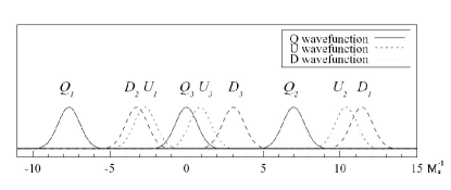
Figure 1: Fermion distribution in extra dimensions in the illustrative model of geog .

We also have some freedom in choosing the extra-dimensional profile of the quark wave functions. We will consider two cases: (1) each quark is sharply localized at a single point in the extra dimensions (i.e. Dirac delta function profile) and (2) the quarks have bulk wave functions with a Gaussian profile. In case (2), we take the width of the Gaussian profile to be $\Delta=M_{\star}^{-1}$.

Since Higgs and gauge bosons (gluons, W’s, Z’s and photons) must interact with all the quarks (and leptons) they can not be localized at one point but have to propagate between the sheets where the fermions are localized. We take the wave functions of these particles to be uniform across the full brane.

Finally, gravitons are not confined to the mini-bulk defined by the standard model thick brane (which may contain several sub-branes where different fermions are localized), but can propagate everywhere in the full bulk.

III Black hole production cross section

Consider two particles colliding with a center of mass energy $E_{CM}$. They will also have an angular momentum $J$ in their center of mass frame. If the impact parameter between the two colliding particles is smaller than the diameter of the horizon of an $(n+1)$-dimensional black hole of mass $M=E_{CM}$ and angular momentum J,

$$b<2r_{h}(n,M,J),$$ (1)

then a black hole will form BHacc . We can say that the incoming particles interacted via non-linear quantum gravity interactions. Since the incoming particles in question are highly relativistic (therefore there is no gravitational focusing), the cross section for this process is precisely equal to the interaction area $\pi(2r_{h})^{2}$.

In our case, where the incident particles are separated in both the ordinary and the extra dimensions, they will have a non-zero impact parameter $b_{e}$ in the bulk directions. No black hole will therefore be formed if their minimal four-dimensional separation (along the brane) exceeds $\sqrt{4r_{h}^{2}(n,E_{CM},J)-b_{e}^{2}}$. The black hole production cross section will therefore be

$$\sigma_{production}(E_{CM},J)=\pi(4r_{h}^{2}(n,E_{CM},J)-b_{e}^{2}).$$ (2)

This cross section is smaller than the usually quoted $\pi 4r_{s}^{2}(n,E_{CM})$ , both because of the effect of the extra-dimensional separation, $b_{e}$, and because the horizon radius, $r_{h}$, is smaller than the Schwarzschild radius, $r_{s}$, whenever $J\neq 0$.

III.1 The impact parameter

The total black hole production cross section depends on the maximal impact parameter between two particles that can yield a black hole of a certain mass – twice the horizon radius of the black hole with the combined center-of-mass energy and angular momentum of the two particles. We must therefore determine this horizon radius.

In Boyer-Lindquist coordinates, the metric for an $(n+1)$-dimensional black hole with angular momentum parallel to the z-axis is:

$$ds^{2} = \left(1-\frac{\mu r^{4-n}}{\Sigma(r,\theta)}\right)dt^{2}$$ (3)

$$- \sin^{2}\theta\left(r^{2}+a^{2}\left(+\sin^{2}\theta\frac{\mu r^{4-n}}{\Sigma(r,\theta)}\right)\right)d\phi^{2}$$

$$+ 2a\sin^{2}\theta\frac{\mu r^{4-n}}{\Sigma(r,\theta)}dtd\phi$$

$$- \frac{\Sigma}{\Delta}dr^{2}-\Sigma d\theta^{2}-r^{2}cos^{2}\theta d^{n-3}\Omega$$

where

$$\Sigma=r^{2}+a^{2}cos^{2}\theta$$

$$\Delta=r^{2}+a^{2}-\mu r^{4-n}.$$ (4)

$$M=\frac{(n-1)A_{n-1}}{16\pi G_{n}}\mu$$ (5)

is the mass of the black hole, and

$$J=\frac{2Ma}{n-1}$$ (6)

is its angular momentum.

Here

$$A_{n-1}=\frac{2\pi^{(n-1)/2}}{\Gamma((n-1)/2)}$$ (7)

is the hyper-surface area of a $(n-1)$-dimensional unit sphere.

The higher dimensional gravitational constant $G_{n}$ is defined as

$$G_{n}=\frac{\pi^{n-4}}{4M_{\star}^{n-1}}$$ (8)

The horizon occurs when $\Delta=0$. That is at a radius given implicitly by

$$r^{(n)}_{h}=\left[\frac{\mu}{1+(a/r^{(n)}_{h})^{2}}\right]^{\frac{1}{n-2}}=\frac{r^{(n)}_{s}}{\left[1+(a/r^{(n)}_{h})^{2}\right]^{\frac{1}{n-2}}}.$$ (9)

Here

$$r^{(n)}_{s}=\mu^{1/(n-2)}.$$ (10)

is the Schwarzschild radius of an $(n+1)$-dimensional black hole. That is

$$r^{(n)}_{s}(us,n,M_{pl})=k(n)M_{pl}^{-1}[\sqrt{us}/M_{pl}]^{1/(n-2)}$$ (11)

$$k(n)\equiv\left[2^{n-3}{\pi}^{(n-6)/2}\frac{\Gamma[n/2]}{n-1}\right]^{1/(n-2)}$$ (12)

If two highly relativistic particles collide with center of mass energy $E_{C}M$, and total impact parameter $b$, then their angular momentum in the center of mass frame before the collision is $J_{in}=bE_{CM}/2$. Suppose that the black hole is formed initially retaining all this energy and angular momentum. Then the mass and angular momentum of the black hole will be $M=M_{in}=\sqrt{s^{\prime}}$ and $J=J_{in}$. A black hole will form if:

$$b<2r^{(n)}_{h}(M_{in},J_{in})\,.$$ (13)

Therefore the maximum impact parameter satisfies

$$b_{max}=2r^{(n)}_{h}(E_{CM},b_{max}E_{CM}/2)\,.$$ (14)

We see that $b_{max}$ is a function of both $E_{CM}$ and the number of dimensions, $n$ ida .

Using equation (9), we can rewrite condition (14)

$$0=\left(\frac{b_{max}}{2}\right)^{2}+\left(\frac{n-1}{4}{b_{max}}\right)^{2}-\mu\left(\frac{b_{max}}{2}\right)^{-d+1}.$$ (15)

We thus obtain for the maximum value of the impact parameter

$$b_{max}(E_{CM};n)=2\frac{r^{(n)}_{s}(E_{CM})}{\left[1+\left(\frac{n-1}{2}\right)^{2}\right]^{1\over{n-2}}}\,.$$ (16)

This result was obtained in ida .

III.2 Cross section when quarks are not separated in bulk directions

If the quarks are not separated in the bulk directions (i.e. $b_{e}=0$), but rather all the standard model particles are localized at a single point in the bulk, then the geometric cross section for black hole production is $\pi(4r_{h}^{2}(n,E_{CM},J))$. The presence of $d$ extra dimensions changes only the value of the horizon radius, as per equation (16).

At the LHC, each proton will have $E=7$TeV in the COM frame. Therefore, the total proton-proton center of mass energy will be $\sqrt{s}=14$TeV. If two partons have energy $vE$ and $\frac{uE}{v}$, much greater than their respective masses, then the parton-parton collision will have

$$s^{\prime}=|p_{i}+p_{j}|^{2}=|v(E,E)+\frac{u}{v}(E,-E)|^{2}=4uE^{2}=us\,.$$ (17)

The center of mass energy for these two partons will be $\sqrt{us}$, as will be the 4-momentum transfer $Q^{2}$. The largest impact parameter between the two particles that can form a black hole with this mass will be $2r_{h}$.

The total proton-proton cross section for black hole production is therefore

$$\sigma^{pp\to BH}(s;n,M_{\star})=\int_{M_{\star}^{2}/s}^{1}\!\!\!\!du\int_{u}^{1}\frac{dv}{v}\pi\left[b_{max}(\sqrt{us})\right]^{2}$$

$$\quad\quad\times\sum_{ij}f_{i}(v,Q=\sqrt{us})f_{j}(u/v,Q=\sqrt{us})\,.$$ (18)

Here $f_{i}(v,Q)$ is the i-th parton distribution function. Loosely this is the expected number of partons of type i and momentum $vQ$ to be found in the proton in a collision at momentum transfer $Q$. This result was also obtained in ida .

III.3 Cross section when quarks are separated

Next, we consider the case when two partons can be located in different points of the extra dimensions. Denote the wave functions of the particles in the extra dimensions as $f^{(e)}_{i}({\vec{x}_{e}})$ and $f^{(e)}_{j}({\vec{x}_{e}})$ (normalized such that $\int|f^{(e)}_{i}(x_{e})|^{2}d^{n-3}x_{e}=1$). The probability that the particles’ separation in the extra dimensions will be $b_{e}$ is therefore

$$P^{ij}_{e}(b_{e})=\int b_{e}^{n-4}d^{n-4}\Omega_{b_{e}}\int d^{n}x_{e}\left|f_{ei}(\vec{x_{e}})f_{ej}(\vec{x_{e}}+\vec{b_{e}})\right|^{2}.$$ (19)

The $(n-3)$-dimensional integral $\int d^{n-3}x_{e}$ is over all possible positions ${\vec{x}_{e}}$ in the extra dimension; the angular integral , $\int d^{n-4}\Omega_{b_{e}}$ , is over all extra-dimensional orientations of ${\vec{b}_{e}}$. $P_{e}$ can be evaluated analytically in simple cases, such as for Gaussian wave functions.

For a given impact parameter $b$ in the ordinary dimensions, $b_{e}$ can take all possible values from zero to $\sqrt{b_{max}(s^{\prime}=us;n)^{2}-b^{2}}$. The contribution to the total cross section from the impact parameter interval $[b,b+db]$, must therefore be weighted by

$$w^{ij}_{e}(b)=\int_{0}^{\sqrt{b_{max}(\sqrt{us})^{2}-b^{2}}}P^{ij}_{e}(b_{e})db_{e}\,.$$ (20)

Applying this to equation (III.2 ) we obtain

$$\sigma^{pp}(s,n,M_{\star}) =\sum_{ij}\int_{M_{\star}^{2}/s}^{1}du\int_{u}^{1}\frac{dv}{v}\int_{0}^{b_{max}(us;n)}w^{ij}_{e}(b)2\pi bdb$$ (21)

$$\times f_{i}(v,Q)f_{j}(u/v,Q)\,.$$

III.4 The Differential Cross-section, $\frac{d\sigma}{dJ}$

The symmetry group of rotations in $n$ spatial dimensions, $SO(n)$ has $\left[n/2\right]$ (the integer part of $n/2$) Casimir operators. This means that there are $\left[n/2\right]$ independent planes of rotations with the same number of parameters of rotation. In the usual ($3+1$)-dimensional case, $n=3$, so there is only one parameter of rotation.

In general, angular momentum is defined as:

$$J^{ij}=\int d^{N}x(x^{i}T^{j0}-x^{j}T^{i0})$$ (22)

where $T^{ij}$ is the momentum density.

Thus, in general, there is a single plane of rotation located within the brane directions and can be one or more planes of rotation extending into the extra dimensions. However, in the case at hand, there are only two particles involved in the collision, with linear momentum along the brane. They move towards each other along two lines that, assuming a non-zero impact parameter, define a single plane. Therefore, assuming our black hole initially carries only the energy and angular momentum of these progenitors, we can always redefine our coordinate system so that the black hole has only one plane of rotation (with a single parameter of rotation). Of course, if $b_{e}\neq 0$, this plane of rotation will be at an angle with respect to the brane. There will therefore be a non-zero bulk component of the angular momentum.

Consider two relativistic particles with center-of-mass energy $s^{\prime}=\sqrt{us}$. In the center of mass frame, each has energy $s^{\prime}/2$, and momentum $\pm s^{\prime}/2$. The angular momentum of the system about its center of mass is

$$J=2\frac{s^{\prime}}{2}\frac{b}{2}=\frac{\sqrt{us}b}{2}.$$ (23)

Since

$$\left(\frac{d\sigma}{db}\right)_{\!\!s^{\prime}}=2\pi b,$$ (24)

therefore

$$\left(\frac{d\sigma}{dJ}\right)_{\!\!s^{\prime}}=\frac{4\pi b}{\sqrt{us}}=\frac{8\pi J}{us}$$ (25)

Eq. (25) is valid for any two partons. For the total cross section, we need to sum over all partons and integrate over all parton momenta.

Combining Eq. (21) and Eq. (25), the cross section change with the brane component of angular momentum becomes

$$\left(\frac{d\sigma^{pp}}{dJ}\right)_{\!\!s} = \sum_{ij}\int_{\max(\frac{M_{\star}^{2}}{s},\frac{4J^{2}}{b^{2}s})}^{1}du\int^{1}_{u}\frac{dv}{v}\frac{8\pi J}{us}w^{ij}_{e}\left(b=\frac{2J}{\sqrt{us}}\right)$$ (26)

$$\times f_{i}(v,Q=\sqrt{us})f_{j}(u/v,Q=\sqrt{us})$$

Similarly, the bulk component of the angular momentum is

$$J_{e}=\frac{\sqrt{us}b_{e}}{2}\,.$$ (27)

Therefore,

$$\left(\frac{d\sigma^{pp}}{dJ_{e}}\right)_{\!\!s}\!\! = \!\!\sum_{ij}\int_{\frac{M_{\star}^{2}}{s}}^{1}du\int^{1}_{u}\frac{dv}{v}\left[P^{ij}_{e}\left(b_{e}\right)\pi\left(b_{max}(\sqrt{us})^{2}-b_{e}^{2}\right)\right]$$ (28)

$$\times f_{i}(v,Q=\sqrt{us})f_{j}(u/v,Q=\sqrt{us}),$$

where $b_{e}=2J_{e}/\sqrt{us}$.

IV Results

IV.1 Cross-section decreases with inter-quark spacing

As two partons are separated in the extra dimensions, their maximum separation along the brane directions becomes smaller, as does the associated black hole production cross section. Thus, the black hole production cross-section is reduced in split-brane models compared to the case where all the quarks and gluons are localized on the same thin brane.

Figure 2: Ratio of black hole production cross-section for the $(4+1)$-dimensional split fermion model to the black hole production cross-section for a $(4+1)$-dimensional model with all the standard model particles localized at a single point, ($\sigma_{split}/\sigma_{nosplit}$) as a function of the size of the extra dimension. The fermion wave functions in both cases are taken to be delta-functions. In the split fermion model, the gluons are permitted to move freely in the thick brane.

As previously mentioned, the extra-dimensional profile of quark wave functions is not well known. We consider two cases: delta-function profiles, and Gaussian profiles.

We first consider the case where the quarks are sharply localized at some point in the extra-dimensional space, with Dirac delta function wave-functions. Gluons can freely propagate between the sheets where quarks are localized, and are taken to have flat (uniform) profiles. The relative location of the quarks is initially set as in our illustrative split-fermion model (section “An illustrative model”). We want to study how the cross section decreases as the separation between the quarks (which we call the size of the extra dimension) increases. So, we change the size of the extra dimension by rescaling the distance between the quarks, while keeping the fundamental energy scale $M_{\star}$ fixed. In Fig. 2, we plot, as a function of the size (in units of $(1{\rm TeV})^{-1}$) of a single extra dimension, the ratio of the black hole production cross section in the split-fermion model to the cross-section in a model with all standard model particles localized at a single point. We do this for a variety of fundamental energy scales from $1$TeV to $10$TeV.

If the size of the extra dimension is smaller than the size of the black hole produced, then the split fermion model is indistinguishable from the un-split model. Therefore the ratio of the cross section in these two cases approaches unity. As the size of the extra dimension increases, and the separation between fermions increases in the split-fermion model, the maximum $(3+1)$-dimensional impact parameter that results in black hole creation decreases. (It is $\sqrt{4r_{h}^{2}-b_{e}^{2}}$ as opposed to $r_{h}$ in the unsplit model.) Therefore, the cross section ratio decreases. The production of smaller mass black holes is affected more than the production of large black holes.

The higher $M_{\star}$, the more rapidly the split fermion black hole production cross section decreases with the increasing size of the extra dimension. This decline ceases when the size of the extra dimension exceeds the size of the black hole. Beyond that point, fermions that are not at the same location in the extra dimension will be too far to interact to form a black hole. Gluons will still contribute but their interaction is also suppressed by the size of the extra dimension. For $(4+1)$ dimensions, the suppression factor is the ratio of the black hole horizon $r_{h}$ to the size $L$ of the extra dimension. Interactions among fermions that are co-located in the extra dimensions will clearly make the dominant contribution, eg. uu and dd type of interaction. The cross section ratio therefore becomes a fixed number, which is however different for different values of $M_{\star}$, because of energy dependent PDF’s. The reason is that as $M_{\star}$ increases, gluon contribution decreases in the non-split case, and since the non-split cross section is in the denominator, the cross section ratio increases.

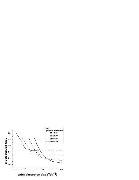
Figure 3: As in figure 2, we show the ratio of black hole production cross-section for the $(4+1)$-dimensional split fermion model to the black hole production cross-section for a $(4+1)$-dimensional model with all the standard model particles localized at a single point, ($\sigma_{split}/\sigma_{nosplit}$) as a function of the size of the extra dimension. Unlike in figure 2, the fermion wave functions are taken to be Gaussian.

We next consider the case where the fermion wave-functions in the extra dimension are Gaussian. The gluons can move freely in the extra dimension between the sheets where quarks are localized, and are taken to have flat (uniform) profiles.. As before, so long as the size of the extra dimension is very small, the ratio of the black hole production cross-section in this split brane model to the production cross section in a single brane model is very close unity. At an intermediate size of the extra dimension, the cross section in the split fermion model is again suppressed due to the reduced interaction range. As expected, the decay is slower for the Gaussian wave function than for the delta function. For larger distances between the fermions the ratio decays again with $r_{h}/L$. These features can be seen in Fig. 3.

Finally, we consider the thick brane case. Strictly speaking, this is not one of the sub-classes of the split fermion model. Rather it is the case where the brane on which the standard model fields are localized is not infinitely thin but has some finite thickness. Here, we take flat (homogeneous) distribution functions for both quarks and the gluons. Some characteristics are the same as for the previous two cases. When the size of the extra dimension is small compared to the size of the produced black holes, there is no difference between the thick and thin brane cases. As the thickness of the brane increases, the cross section ratio decreases very quickly. But for large thickness of the brane (much larger than typical black hole size), there is no specific size of extra dimensions (brane thickness) where the ratio stops decreasing sharply as in the two previous cases. Instead, the cross section ratio decreases like $r_{h}/L$. For higher $M_{\star}$, $r_{h}$ is smaller, and higer $M_{\star}$ curves decay faster. These features can be seen in Fig. 4.

Figure 4: This figure shows the ratio of black hole production cross-section for the $(4+1)$-dimensional thick brane model where all the standard model particles have uniform distribution along the extra dimension, to the black hole production cross-section for a $(4+1)$-dimensional model with all the standard model particles localized at a single point, ($\sigma_{thick}/\sigma_{thin}$) as a function of the size of the extra dimension.

IV.2 Angular momentum distribution

The angular momentum of the black holes produced at the LHC cannot be directly measured. However, a black hole’s angular momentum strongly affects its Hawking radiation, especially through the super-radiance effect described in the introduction. In most analysis of Hawking radiation from mini black holes, the bulk component of angular momentum is neglected. However, in the split fermion model, this assumption cannot be justified. Our results show that the bulk component of angular momentum can be as large as the brane component, thus greatly amplifying bulk radiation (at least in the initial stages after formation, while the black hole is still rotating fast).

We must emphasize that the angular momentum analysis performed here is classical. It is likely that the results and even the conclusions will change if quantum corrections are not negligible.

IV.2.1 One extra dimension

We first consider the $(4+1)$-dimensional case. In Fig. 6, we plot the differential cross-section $\frac{d\sigma}{dJ}$. This encodes the expected number of black holes to be created as a function of their angular momentum. We take $M_{\star}=5TeV$ and fix the size of the extra dimension as $L=10M_{\star}^{-1}$. We we take the fermions to have Gaussian wave functions in the extra dimension. The distributions of both bulk and brane components of the angular momentum are plotted. For comparison, on the same graph, we also show the distribution of the brane component of angular momentum for the the case where fermions are not split.

We see that the cross section in the non-split case increases with angular momentum linearly. After the angular momentum reaches the maximum that the smallest black hole can provide (most of the produced black holes will have the smallest possible mass), the cross section decreases very quickly. To produce higher angular momentum black holes, one needs higher energy partons. From inspection of the parton distribution functions pdfs (Fig. 5), one can see that the number of higher energy partons decreases very quickly. Thus, at very high angular momenta, the cross section will be suppressed.

Figure 5: Parton distribution functions

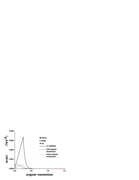
Figure 6: Angular momentum distribution for a $(4+1)$-dimensional model. The fermions have Gaussian profile in the extra dimension. Gluons have uniform (flat) profile in extra dimensions. For comparison, we keep the plot in the non-split case (solid line). $M_{\star}=5TeV$, $L=10M_{\star}^{-1}$.

As expected, in the split fermions case, the cross section is reduced compared to the un-split case. The cross section still reaches its maximum when the angular momentum in the brane directions is comparable to the maximum that the smallest black hole can provide (since most of the produced black holes will be the smallest possible).

Regarding the bulk component of angular momentum, since the cross section will not be suppressed, if the distance between partons in extra dimensions is zero, zero angular momentum will have the highest cross section. However, this is an artifact of one extra dimension. This feature will change if there is more than one extra dimension.

IV.2.2 Two extra dimensions

We next consider the case with two extra dimensions. The fermions again are taken to have Gaussian wave functions in the extra dimensions. ¿From figure 7, we see that the probability distribution of the brane component of the angular momentum behaves similarly as in $(4+1)$-dimensions. Not so the bulk component of the angular momentum. In particular, the most likely value of the bulk component of the angular momentum is no longer zero. When there are two extra dimensions, the probability to find two particles at the same location (which will yield zero bulk angular momentum) becomes very small. Therefore, though one obtains the highest cross section when particles that are not separated in extra space collide, this configuration is unlikely if there is more than one extra dimension.

Figure 7: Angular momentum distribution for a $(5+1)$-dimensional model. The fermions have Gaussian profile in the extra dimensions. Gluons have uniform (flat) profile in extra dimensions. For comparison, we keep the plot in the non-split case (solid line). $M_{\star}=5TeV$, $L=10M_{\star}^{-1}$.

Finally, in Fig. 8, we show the case of a thick brane (flat quark and gluon profiles). The size of the extra dimensions is ${\cal O}(M_{\star}^{-1})$. The brane and bulk angular momentum distributions are very similar in this case. We should first note that in any case most of the produced black holes will have the smallest possible mass (production of heavier black holes is suppressed in proportion to their mass). At distances of the order of the gravitational radius of these small black holes (i.e. $\sim M_{\star}^{-1}$) one does not distinguish much between the brane and bulk directions. Therefore, the difference between the bulk and brane angular momentum distribution is small in this case.

Figure 8: Angular momentum distribution in 5+1D. The fermions and gluons have uniform (flat) profile in extra dimensions. For comparison, we keep the plot in the non-split case (solid line). $M_{\star}=5TeV$, $L=M_{\star}^{-1}$.

V Conclusion

Black hole production at the LHC may be one of the earliest signatures of TeV-scale quantum gravity. This topic has been subject to an extensive investigation HKM ; 1 ; 2 ; 3 ; 4 ; 5 ; 6 ; 7 ; 9 ; 10 ; 11 ; 12 ; 13 ; 14 ; 15 ; 16 ; 17 ; 18 ; 19 ; 20 ; 21 ; 22 ; 23 ; 24 ; 25 ; 26 ; 27 ; 28 ; 29 ; 30 ; 31 ; 32 ; 33 ; 34 ; 35 ; 36 ; 37 ; 37.5 ; 38 ; 39 ; 40 ; 41 ; 42 ; 43 ; 44 ; 45 ; 46 ; 47 ; 48 ; 49 ; 50 ; 51 ; 52 ; 53 . In order to make serious predictions, one needs to work within the context of realistic phenomenologically valid models. In the first place one has to suppress a very rapid quantum gravity mediated proton decay. There are also many other problems related to TeV-scale quantum gravity like large $n-{\bar{n}}$ oscillations, flavor changing neutral currents, large mixing between leptons, etc.. It is widely accepted that so-called ‘split fermion” model (where fermions are localized at different points in extra dimensions) can solve most of these problems.

In this paper we re-examined black holes production and their angular momentum distribution in the context of this model with split fermions. As a consequence of separation of partons in the extra dimensions, we find that the total production cross section is reduced compared with models where all the fermions are localized in the same point in extra dimensions.

Due to the non-zero impact parameter, most of the produced black holes will be rotating. Split fermions imply that the bulk component of the black hole angular momentum can not be neglected and must be taken into account in studies of Hawking radiation from such black holes. In a follow on work (in preparation) with collaborators from the ATLAS consortium we will consider the impact of these and related effects on experimentally measurable quantities.

Acknowledgements:

We thank Cigdem Issever, Nicholas Brett and Jeff Tseng of the Oxford ATLAS group for many productive conversations. GDS is supported in part by fellowships from the John Simon Guggenheim Memorial Foundation and the Beecroft Institute for Particle Astrophysics and Cosmology, Oxford. He thanks the Beecroft Institute and Oxford Physics for their hospitality during the course of this research. This research is supported by a grant from the US DOE to the particle-astrophysics theory group at CWRU.

References

- (1) N. Arkani-Hamed, S. Dimopoulos and G. Dvali, Phys. Lett. B429, 263 (1998).
- (2) T. Banks, W. Fischler, hep-th/9906038 ; S. Dimopoulos, G. Landsberg, Phys. Rev. Lett. 87 161602 (2001) ; S. B. Giddings and S. Thomas, Phys. Rev. D65 056010 (2002)
- (3) J.L. Feng, A.D. Shapere, Phys. Rev. Lett. 88 021303 (2002)
- (4) D. Stojkovic, G. D. Starkman, D.C. Dai, Phys. Rev. Lett 96 041303 (2006)
- (5) N. Arkani-Hamed, S. Dimopoulos, G.R. Dvali, Phys.Rev. D59 086004 (1999); F. C. Adams, G. L. Kane, M. Mbonye, M. J. Perry, Int.J.Mod.Phys. A16 2399 (2001); D. Stojkovic, G. D. Starkman, F. C. Adams, gr-qc/0604072
- (6) L.M. Krauss and F. Wilczek, Phys. Rev. Lett. 62, 1221 (1989).
- (7) L.E. Ibanez and G.G. Ross, Nucl. Phys. B368, 3 (1992).
- (8) N. Arkani-Hamed, M. Schmaltz, Phys. Rev. D61 033005 (2000); N. Arkani-Hamed, Y. Grossman, M. Schmaltz, Phys. Rev. D61 115004 (2000)
- (9) Eugene A. Mirabelli and Martin Schmaltz Phys.Rev.D61 113011 (2000)
- (10) R. Emparan, G. T. Horowitz, R. C. Myers Phys.Rev.Lett.85 499 (2000)
- (11) D. N. Page, Phys. Rev. D13 198 (1976); Phys. Rev. D14 3260 (1976).
- (12) V. Frolov and I. Novikov. Black Hole Physics: Basic Concepts and New Developments (Kluwer Academic Publ.), 1998.
- (13) V. P. Frolov, D. Stojkovic, Phys. Rev. D67 084004 (2003); Phys. Rev. D68 064011 (2003)
- (14) V. Frolov, D. Stojkovic, Phys. Rev. Lett. 89 151302 (2002); Phys. Rev. D66 084002 (2002); D. Stojkovic, Phys.Rev.Lett. 94 011603 (2005)
- (15) D. Stojkovic, JHEP 0409:061 (2004)
- (16) D. Ida, K. Oda, S. C. Park, Phys.Rev.D67 064025 (2003) Erratum-ibid.D69 049901 (2004); hep-ph/0312061
- (17) J. Pumplin et al. JHEP 0207, 012 (2002)[hep-ph/0201195]; D. Stump et al., JHEP 0310, 046 (2003)[hep-ph/0303013].
- (18) T. Han, G. D. Kribs and B. McElrath, Phys. Rev. Lett. 90, 031601 (2003)
- (19) A. Flachi, O. Pujolas, M. Sasaki, T. Tanaka, hep-th/0601174; A. Flachi, T. Tanaka, Phys. Rev. Lett. 95 161302 (2005)
- (20) T. G. Rizzo, hep-ph/0601029; hep-ph/0510420; JHEP 0501 028 (2005)
- (21) D.K. Park, hep-th/0512021; hep-th/0511159; hep-th/0603224
- (22) M. Casals, P. Kanti, E. Winstanley, hep-th/0511163
- (23) R. da Rocha, C. H. Coimbra-Araujo, JCAP 0512 009 (2005)
- (24) A.S. Cornell, W. Naylor, M. Sasaki; hep-th/0510009
- (25) J. Grain, A. Barrau, P. Kanti, Phys.Rev.D72 104016 (2005)
- (26) H. Yoshino, T. Shiromizu, M. Shibata, Phys.Rev. D72 084020 (2005)
- (27) G. Duffy, C. Harris, P. Kanti, E. Winstanley, JHEP 0509 049 (2005)
- (28) E. Jung, D.K. Park, Nucl.Phys. B731 171 (2005)
- (29) L. Lonnblad, M. Sjodahl, T. Akesson, JHEP 0509 019 (2005)
- (30) J.I. Illana, M. Masip, D. Meloni, Phys.Rev.D72 024003 (2005)
- (31) E. Jung, S. Kim, D.K. Park, Phys.Lett. B619 347 (2005); Phys.Lett. B614 78 (2005)
- (32) H. Yoshino, V. S. Rychkov, Phys.Rev. D71 104028 (2005)
- (33) A.S. Majumdar, N. Mukherjee, Int.J.Mod.Phys. D14 1095 (2005); astro-ph/0403405
- (34) A. Perez-Lorenzana, hep-ph/0503177
- (35) D. Ida, K. Oda, S. C. Park, Phys.Rev. D71 124039 (2005);hep-th/0602188
- (36) V. P. Frolov, D. V. Fursaev, D. Stojkovic, Class. Quant. Grav. 21 3483 (2004); JHEP 0406 057 (2004);
- (37) A.N. Aliev, A.E. Gumrukcuoglu, Phys.Rev. D71 104027 (2005); A.N. Aliev, gr-qc/0505003; A.N. Aliev, V. P. Frolov, Phys.Rev.D69 084022 (2004)
- (38) P. Kanti, J. Grain, A. Barrau, Phys.Rev. D71 104002 (2005); P. Kanti, K. Tamvakis, Phys.Rev. D65 084010 (2002); P. Kanti, J. March-Russell, Phys.Rev.D67 104019 (2003); P. Kanti, Int.J.Mod.Phys.A19 4899 (2004)
- (39) H. Yoshino, Y. Nambu, Phys.Rev. D70 084036 (2004)
- (40) E. F. Eiroa, gr-qc/0511004; Phys.Rev. D71 083010 (2005)
- (41) P. S. Apostolopoulos, N. Brouzakis, E. N. Saridakis, N. Tetradis Phys.Rev. D72 044013 (2005)
- (42) S. Creek, O. Efthimiou, P. Kanti, K. Tamvakis, hep-th/0601126
- (43) D. Stojkovic, Phys.Rev.D67 045012 (2003)
- (44) E. Berti, V. Cardoso, M. Casals, Phys.Rev. D73 024013 (2006)
- (45) M. Vasudevan, K. A. Stevens, Phys.Rev. D72 124008 (2005)
- (46) B. M.N. Carter, I. P. Neupane, Phys.Rev. D72 043534 (2005)
- (47) L. Lonnblad, M. Sjodahl, T. Akesson, JHEP 0509 019 (2005)
- (48) V. Frolov, M. Snajdr and D. Stojkovic, Phys. Rev. D68 044002 (2003);
- (49) M. Nozawa, K. Maeda, Phys.Rev. D71 084028 (2005)
- (50) C. M. Harris, hep-ph/0502005
- (51) Y. Morisawa, D. Ida, Phys.Rev.D71 044022 (2005)
- (52) V. Cardoso, G. Siopsis, S. Yoshida, Phys.Rev. D71 024019 (2005); V. Cardoso, J. P.S. Lemos, Phys.Lett. B621 219 (2005); V. Cardoso, O.J.C. Dias, J. P.S. Lemos, Phys.Rev.D67 064026 (2003); V. Cardoso, O. J.C. Dias, J. L. Hovdebo, R. C. Myers, hep-th/0512277
- (53) A. Cafarella, C. Coriano, T.N. Tomaras, hep-ph/0412037; A. Sheykhi, N. Riazi, hep-th/0605042
- (54) A. Chamblin, F. Cooper, G. C. Nayak, Phys.Rev. D70 075018 (2004); Phys.Rev. D69 065010 (2004)
- (55) G. D. Starkman, D. Stojkovic, M. Trodden, Phys.Rev.Lett. 87 231303 (2001); Phys.Rev.D63 103511 (2001)
- (56) D. Ida, Y. Uchida, Y. Morisawa, Phys.Rev.D67 084019 (2003)
- (57) E.J. Ahn, M. Cavaglia, hep-ph/0511159
- (58) M. Cavaglia, S. Das, Class.Quant.Grav. 21 4511 (2004); M. Cavaglia, S. Das, R. Maartens, Class.Quant.Grav. 20 L205 (2003)
- (59) V. Cardoso, M. Cavaglia, L. Gualtieri, hep-th/0512116
- (60) L. A. Anchordoqui, J. L. Feng, H. Goldberg, A. D. Shapere, Phys.Lett.B594 363 (2004); Phys.Rev.D68 104025 (2003); Phys.Rev.D66 024033 (2002); Phys.Rev.D65 124027 (2002); L. Anchordoqui, H. Goldberg, Phys.Rev.D67 064010 (2003); L. Anchordoqui, T. Han, D. Hooper, S. Sarkar, hep-ph/0508312
- (61) A. Casanova, E. Spallucci, Class.Quant.Grav. 23 R45 (2006)
- (62) J. E. Aman, N. Pidokrajt, Phys.Rev.D73 024017 (2006); S. Wu, Q. Jiang, hep-th/0603082
- (63) U. Harbach, M. Bleicher, hep-ph/0601121
- (64) B. Koch, M. Bleicher, S. Hossenfelder, JHEP 0510 053 (2005); S. Hossenfelder, Phys.Lett. B598 92 (2004)
- (65) M. Fairbairn, hep-ph/0509191
- (66) R. Casadio, B. Harms, Int. J. Mod. Phys. A17 4635 (2002); G.L. Alberghi, R. Casadio, D. Galli, D. Gregori, A. Tronconi, V. Vagnoni, hep-ph/0601243
- (67) P. Davis, hep-th/0602118; P. Krtous, J. Podolsky, Class.Quant.Grav. 23 1603 (2006)
- (68) K.A. Bronnikov, S.A. Kononogov, V.N. Melnikov, gr-qc/0601114
- (69) N. Kaloper, D. Kiley, JHEP 0603 077 (2006)
- (70) A. Lopez-Ortega, Gen.Rel.Grav. 35 1785 (2003)
- (71) S. Hossenfelder, S. Hofmann, M. Bleicher and H. Stoecker, Phys. Rev. D 66, 101502 (2002)