May 2006

TWO PARTICLE CORRELATIONS INSIDE ONE JET

AT “MODIFIED LEADING LOGARITHMIC APPROXIMATION”

OF QUANTUM CHROMODYNAMICS

I: EXACT SOLUTION OF THE EVOLUTION EQUATIONS AT SMALL $\boldsymbol{X}$

Redamy Perez-Ramos

Laboratoire de Physique Théorique et Hautes Energies

Unité Mixte de Recherche UMR 7589

Université Pierre et Marie Curie-Paris6; CNRS; Université Denis Diderot-Paris7

Abstract: We discuss correlations between two particles in jets at high energy colliders and exactly solve the MLLA evolution equations in the small $x$ limit. We thus extend the Fong-Webber analysis to the region away from the hump of the single inclusive energy spectrum. We give our results for LEP, Tevatron and LHC energies, and compare with existing experimental data.

Keywords: Perturbative Quantum Chromodynamics, Particle Correlations in jets, High Energy Colliders

1 INTRODUCTION

Perturbative QCD (pQCD) successfully predicts inclusive energy spectra of particles in jets. To this end it was enough to make one step beyond the leading “Double Logarithmic Approximation” (DLA) which is known to overestimate soft gluon multiplication, and to describe parton cascades with account of first sub-leading single logarithmic (SL) effects. Essential SL corrections to DLA arise from:

$\ast$  the running coupling $\alpha_{s}(k_{\perp}^{2})$;

$\ast$  decays of a parton into two with comparable energies, $z\sim 1$ (the so called “hard corrections”, taken care of by employing exact DGLAP [1] splitting functions);

$\ast$  kinematical regions of successive parton decay angles of the same order of magnitude, $\Theta_{i+1}\sim\Theta_{i}$. The solution to the latter problem turned out to be extremely simple namely, the replacement of the strong angular ordering (AO), $\Theta_{i+1}\ll\Theta_{i}$, imposed by gluon coherence in DLA , by the exact AO condition $\Theta_{i+1}\leq\Theta_{i}$ (see [2] and references therein). The corresponding approximation is known as MLLA (Modified Leading Logarithm Approximation) and embodies the next-to-leading correction, of order $\gamma_{0}^{2}$, to the parton evolution “Hamiltonian”, $\gamma_{0}\propto\sqrt{\alpha_{s}}$ being the DLA multiplicity anomalous dimension [2].

So doing, single inclusive charged hadron spectra (dominated by pions) were found to be mathematically similar to that of the MLLA parton spectrum, with an overall proportionality coefficient ${\cal K}^{ch}$ normalizing partonic distributions to the ones of charged hadrons; ${\cal K}^{ch}$ depends neither on the jet hardness nor on the particle energy. This finding was interpreted as an experimental confirmation of the Local Parton–Hadron Duality hypothesis (LPHD) (for a review see [3][4] and references therein). However, in the ratio of two particle distribution and the product of two single particle distributions that determine the correlation, this non-perturbative parameter cancels. Therefore, one expects this observable to provide a more stringent test of parton dynamics. At the same time, it constitutes much harder a problem for the naive perturbative QCD (pQCD) approach.

The correlation between two soft gluons was tackled in DLA in [5]. The first realistic prediction with account of next-to-leading (SL) effects was derived by Fong and Webber in 1990 [6]. They obtained the expression for the two particle correlator in the kinematical region where both particles were close in energy to the maximum (”hump”) of the single inclusive distribution. In [7] this pQCD result was compared with the OPAL $e^{+}e^{-}$ annihilation data at the $Z^{0}$ peak: the analytical calculations were found to have largely overestimated the measured correlations.

In this paper we use the formalism of jet generating functionals [8] to derive the MLLA evolution equations for particle correlators (two particle inclusive distributions). We then use the soft approximation for the energies of the two particle by neglecting terms proportional to powers of $x_{1},x_{2}\ll 1$ ($x$ is the fraction of the jet energy carried away by the corresponding particle). Thus simplified, the evolution equations can be solved iteratively and their solutions are given explicitly in terms of logarithmic derivatives of single particle distributions.

This allows us to achieve two goals. First, we generalize the Fong–Webber result by extending its domain of application to the full kinematical range of soft particle energies. Secondly, by doing this, we follow the same logic as was applied in describing inclusive spectra namely, treating exactly approximate evolution equations. Strictly speaking, such a solution, when formally expanded, inevitably bears sub-sub-leading terms that exceed the accuracy with which the equations themselves were derived. This logic, however, was proved successful in the case of single inclusive spectra [9], which demonstrated that MLLA equations, though approximate, fully take into account essential physical ingredients of parton cascading: energy conservation, coherence, running coupling constant. Applying the same logic to double inclusive distributions should help to elucidate the problem of particle correlations in QCD jets.

The paper is organized as follows.

$\bullet$ in section 2 we recall the formalism of jet generating functionals and their evolution equations; we specialize first to inclusive energy spectrum, and then to 2-particle correlations;

$\bullet$ in section 3, we solve exactly the evolution equations in the low energy (small $x$) limit; how various corrections are estimated and controlled is specially emphasized;

$\bullet$ section 4 is dedicated to correlations in a gluon jet; the equation to be solved iteratively is exhibited, and an estimate of the order of magnitudes of various contributions is given;

$\bullet$ section 5 is dedicated to correlations in a quark jet, and follows the same lines as section 4;

$\bullet$ in section 6 we give all numerical results, for LEP-I, Tevatron and LHC. They are commented, compared with Fong-Webber for OPAL, but all detailed numerical investigations concerning the size of various corrections is postponed, for the sake of clarity, to appendix E;

$\bullet$ a conclusion summarizes this work.

Six appendices provide all necessary theoretical demonstrations and numerical investigations.

$\bullet$ in appendix A and B we derive the exact solution of the evolution equations for the gluon and quark jet correlators;

$\bullet$ appendix C is a technical complement to subsection 4.2;

$\bullet$ in appendix D we demonstrate the exact solution of the MLLA evolution equation for the inclusive spectrum and give analytic expressions for its derivatives;

$\bullet$ appendix E is dedicated to a numerical analysis of all corrections that occur in the iterative solutions of the evolution equations;

$\bullet$ in appendix F we perform a comparison between DLA and MLLA correlators.

2 EVOLUTION EQUATIONS FOR JET GENERATING FUNCTIONALS

Consider (see Fig. 1) a jet generated by a parton of type $A$ (quark or gluon) with 4-momentum $p=(p_{0}\equiv E,\vec{p})$.

Figure 1: Two-particle correlations and Angular Ordering

A generating functional $Z(E,\Theta;\{u\})$ can be constructed [8] that describes the azimuth averaged parton content of a jet of energy $E$ with a given opening half-angle $\Theta$; by virtue of the exact angular ordering (MLLA), it satisfies the following integro-differential evolution equation [2]

$$\frac{d}{d\ln\Theta}Z_{A}\left(p,\Theta;\{u\}\right)\!\! \!\!=\!\! \!\!\frac{1}{2}\sum_{B,C}\int_{0}^{1}dz\>\Phi_{A}^{B[C]}(z)\ \frac{\alpha_{s}\left(k^{2}_{\perp}\right)}{\pi}$$ (2)

$$\Big{(}Z_{B}\big{(}zp,\Theta;\{u\}\big{)}\ Z_{C}\big{(}(1-z)p,\Theta;\{u\}\big{)}-Z_{A}\big{(}p,\Theta;\{u\}\big{)}\Big{)};$$

in (2), $z$ and $(1-z)$ are the energy-momentum fractions carried away by the two offspring of the $A\to BC$ parton decay described by the standard one loop splitting functions

$$\Phi_{q}^{q[g]}(z)=C_{F}\,\frac{1+z^{2}}{1-z},\quad\Phi_{q}^{g[q]}(z)=C_{F}\,\frac{1+(1-z)^{2}}{z},$$ (3)

$$\Phi_{g}^{q[\bar{q}]}(z)=T_{R}\left(z^{2}+(1-z)^{2}\right),\quad\Phi_{g}^{g[g]}(z)=2C_{A}\left(\frac{1-z}{z}+\frac{z}{1-z}+z(1-z)\right),$$ (4)

$$C_{A}=N_{c},\quad C_{F}=(N_{c}^{2}-1)/2N_{c},\quad T_{R}=1/2,$$ (5)

where $N_{c}$ is the number of colors; $Z_{A}$ in the integral in the r.h.s. of (2) accounts for 1-loop virtual corrections, which exponentiate into Sudakov form factors.

$\alpha_{s}(q^{2})$ is the running coupling constant of QCD

$$\alpha_{s}(q^{2})=\frac{4\pi}{4N_{c}\beta\ln\displaystyle\frac{q^{2}}{\Lambda^{2}_{QCD}}},$$ (6)

where $\Lambda_{QCD}\approx$ a few hundred $MeV$’s is the intrinsic scale of QCD, and

$$\beta=\frac{1}{4N_{c}}\Big{(}\frac{11}{3}N_{c}-\frac{4}{3}n_{f}T_{R}\Big{)}$$ (7)

is the first term in the perturbative expansion of the $\beta$ function, $n_{f}$ the number of light quark flavors.

If the radiated parton with 4-momentum $k=(k_{0},\vec{k})$ is emitted with an angle $\Theta$ with respect to the direction of the jet, one has ($k_{\perp}$ is the modulus of the transverse trivector $\vec{k}_{\perp}$ orthogonal to the direction of the jet) $k_{\perp}\simeq|\vec{k}|\Theta\approx k_{0}\Theta\approx zE\Theta$ when $z\ll 1$ or $(1-z)E\Theta$ when $z\to 1$, and a collinear cutoff $k_{\perp}\geq Q_{0}$ is imposed.

In (2) the symbol $\{u\}$ denotes a set of probing functions $u_{a}(k)$ with $k$ the 4-momentum of a secondary parton of type $a$. The jet functional is normalized to the total jet production cross section such that

$$Z_{A}(p,\Theta;u\equiv 1)=1;$$ (8)

for vanishingly small opening angle it reduces to the probing function of the single initial parton

$$Z_{A}(p,\Theta\to 0;\{u\})=u_{A}(k\equiv p).$$ (9)

To obtain exclusive $n$-particle distributions one takes $n$ variational derivatives of $Z_{A}$ over $u(k_{i})$ with appropriate particle momenta, $i=1\ldots n$, and sets $u\equiv 0$ after wards; inclusive distributions are generated by taking variational derivatives around $u\equiv 1$.

2.1 Inclusive particle energy spectrum

The probability of soft gluon radiation off a color charge (moving in the $z$ direction) has the polar angle dependence

$$\frac{\sin\theta\,d\theta}{2(1-\cos\theta)}=\frac{d\sin(\theta/2)}{\sin(\theta/2)}\simeq\frac{d\theta}{\theta};$$

therefore, we choose the angular evolution parameter to be

$$Y=\ln\frac{2E\sin(\Theta/2)}{Q_{0}}\Rightarrow dY=\frac{d\sin(\Theta/2)}{\sin(\Theta/2)};$$ (10)

this choice accounts for finite angles ${\cal O}(1)$ up to the full opening half-angle $\Theta=\pi$, at which

$$Y_{\Theta=\pi}=\ln\frac{2E}{Q_{0}},$$

where $2E$ is the center-of-mass annihilation energy of the process $e^{+}e^{-}\to q\bar{q}$. For small angles (10) reduces to

$$Y\simeq\ln\frac{E\Theta}{Q_{0}},\quad\Theta\ll 1,\quad\frac{d}{dY}=\frac{d}{d\ln\Theta},$$ (11)

where $E\Theta$ is the maximal transverse momentum of a parton inside the jet with opening half-angle $\Theta$.

To obtain the inclusive energy distribution of parton $a$ emitted at angles smaller than $\Theta$ with momentum $k_{a}$, energy $E_{a}=xE$ in a jet $A$, i.e. the fragmentation function ${D}_{A}^{\,a}(x,Y)$, we take the variational derivative of (2) over $u_{a}(k)$ and set $u\equiv 1$ (which also corresponds to $Z=1$) according to

$$x{D_{A}^{a}}(x,Y)=E_{a}\frac{\delta}{\delta u(k_{a})}Z_{A}\left(k,\Theta;\left\{u\right\}\right)\Big{|}_{u=1},$$ (12)

where we have chosen the variables $x$ and $Y$ rather than $k_{a}$ and $\Theta$.

Two configurations must be accounted for: $B$ carrying away the fraction $z$ and $C$ the fraction $(1-z)$ of the jet energy, and the symmetric one in which the role of $B$ and $C$ is exchanged. Upon functional differentiation they give the same result, which cancels the factor $1/2$. The system of coupled linear integro-differential equations that comes out is

$$\frac{d}{dY}\,x{D}^{a}_{A}(x,Y)=\int_{0}^{1}dz\sum_{B}\Phi_{A}^{B}(z)\,\frac{\alpha_{s}}{\pi}\left[\frac{x}{z}{D}^{a}_{B}\left(\frac{x}{z},Y+\ln z\right)-\frac{1}{2}x{D}^{a}_{A}(x,Y)\right].$$ (13)

We will be interested in the region of small $x$ where fragmentation functions behave as

$$x{D}(x)\stackrel{{\scriptstyle x\ll 1}}{{\sim}}\rho(\ln x),$$ (14)

with $\rho$ a smooth function of $\ln x$. Introducing logarithmic parton densities

$$Q=x{D}^{\,a}_{Q}(x,Y),\quad G=x{D}^{\,a}_{G}(x,Y),$$ (15)

respectively for quark and gluon jets, we obtain from (13)

$$Q_{y}\equiv\frac{dQ}{dy}\!\! \!\!=\!\! \!\!\int_{0}^{1}dz\>\frac{\alpha_{s}}{\pi}\>\Phi_{q}^{g}(z)\>\bigg{[}\Big{(}Q(1-z)-Q\Big{)}+G(z)\bigg{]},$$ (16)

$$G_{y}\equiv\frac{dG}{dy}\!\! \!\!=\!\! \!\!\int_{0}^{1}dz\>\frac{\alpha_{s}}{\pi}\>\bigg{[}\Phi_{g}^{g}(z)\Big{(}G(z)-zG\Big{)}+n_{f}\;\Phi_{g}^{q}(z)\,\Big{(}2Q(z)-G\Big{)}\bigg{]},$$ (17)

where, for the sake of clarity, we have suppressed $x$ and $Y$ and only kept the dependence on the integration variable $z$, e.g.,

$$G(z)\equiv\frac{x}{z}{D}^{a}_{G}\bigg{(}\frac{x}{z},Y+\ln z\bigg{)},$$ (18)

such that

$$G=G(1),\quad Q=Q(1).$$ (19)

Some comments are in order concerning these equations.

• We chose to express the derivative with respect to the jet opening angle $\Theta$ on the l.h.s.’s of equations (16)(17) in terms of

  $$y\equiv Y-\ell=\ln\frac{xE\Theta}{Q_{0}}=\ln\frac{E_{a}\Theta}{Q_{0}},\quad\ell\equiv\ln\frac{1}{x}=\ln\frac{E}{E_{a}},$$ (20)

  instead of $Y$ defined in (10). The variable $y$ is convenient for imposing the collinear cutoff condition $k_{\perp}\simeq xE\sin\theta\geq Q_{0}$ since, for small angles, it translates simply into $y\geq 0$;

• to obtain (16) one proceeds as follows. When $B$ is a quark in (13) , since $A$ is also a quark, one gets two contributions: the real contribution ${D_{B=q}^{a}}$ and the virtual one $-\frac{1}{2}{D_{A=q}^{a}}$;

  • in the virtual contribution, since $\Phi_{q}^{q}(z)=\Phi_{q}^{g}(1-z)$, the sum over $B$ cancels the factor $1/2$;

  • in the real contribution, when it is a quark, it is associated with $\Phi_{q}^{q}(z)$ and, when it is a gluon, with $\Phi_{q}^{g}(z)$; we use like above the symmetry $\Phi_{q}^{q}(z)=\Phi_{q}^{g}(1-z)$ to only keep one of the two, namely $\Phi_{q}^{q}$, at the price of changing the corresponding $D(z)$ into ${D}(1-z)$;

• to obtain (17), one goes along the following steps; now $A=g$ and $B=q$ or $g$;

  • like before, the subtraction term does not depend on $B$ and is summed over $B=q$ and $B=g$, with the corresponding splitting functions $\Phi_{g}^{q}$ and $\Phi_{g}^{g}$. In the term $\Phi_{g}^{g}$, using the property $\Phi_{g}^{g}(z)=\Phi_{g}^{g}(1-z)$ allows us to replace $\frac{1}{2}\int_{0}^{1}dz\Phi_{g}^{g}(z)=\int_{0}^{1}z\Phi_{g}^{g}(z)$. This yields upon functional differentiation the $-zG$ term in (17). For $B=q$, $2n_{f}$ flavors ($n_{f}$ flavors of quarks and $n_{f}$ flavors of anti-quarks) yield identical contributions, which, owing to the initial factor $1/2$ finally yields $n_{f}$;

  • concerning the real terms, $\Phi_{g}^{g}G$ in (17) comes directly from $\Phi_{g}^{g}\frac{x}{z}{D_{g}^{a}}$ in (13). For $B=q$, $2n_{f}$ flavors of quarks and antiquarks contribute equally since at $x\ll 1$ sea quarks are produced via gluons . This is why we have multiplied $Q(z)$ by $2n_{f}$ in (17).

Now we recall that both splitting functions $\Phi_{q}^{g}(z)$ and $\Phi_{g}^{g}$ are singular at $z=0$; the symmetric gluon-gluon splitting $\Phi_{g}^{g}(z)$ is singular at $z=1$ as well. The latter singularity in (17) gets regularized by the factor $\big{(}G(z)-zG\big{)}$ which vanishes at $z\to 1$. This regularization can be made explicit as follows

$$\int_{0}^{1}dz\Phi_{g}^{g}(z)\>\Big{(}G(z)-zG\Big{)}\equiv\int_{0}^{1}dz\Phi_{g}^{g}(z)\>\bigg{[}(1-z)G(z)+z\Big{(}G(z)-G\Big{)}\bigg{]};$$

since $\Phi_{g}^{g}(z)=\Phi_{g}^{g}(1-z)$, while leaving the first term $\int_{0}^{1}dz\Phi_{g}^{g}(z)(1-z)G(z)$ unchanged, we can rewrite the second

$$\int_{0}^{1}dz\Phi_{g}^{g}(z)z\Big{(}G(z)-G\Big{)}=\int_{0}^{1}dz\Phi_{g}^{g}(z)(1-z)\Big{(}G(1-z)-G\Big{)},$$

such that, re-summing the two, $(1-z)$ gets factorized and one gets

$$\int_{0}^{1}dz\Phi_{g}^{g}(z)\>\Big{(}G(z)-zG\Big{)}=\int_{0}^{1}dz\Phi_{g}^{g}(z)(1-z)\bigg{[}G(z)+\Big{(}G(1-z)-G\Big{)}\bigg{]}.$$ (21)

Terms proportional to $G(z)$ on r.h.s.’s of equations (16)(17) remain singular at $z\!\to\!0$ and produce enhanced contributions due to the logarithmic integration over the region $x\ll z\ll 1$.

Before discussing the MLLA evolution equations following from (16) and (17), let us derive similar equation for two particle correlations inside one jet.

2.2 Two parton correlations

We study correlation between two particles with fixed energies $x_{1}=\omega_{1}/E$, $x_{2}=\omega_{2}/E$ ($x_{1}>x_{2}$) emitted at arbitrary angles $\Theta_{1}$ and $\Theta_{2}$ smaller than the jet opening angle $\Theta$. If these partons are emitted in a cascading process, then $\Theta_{1}\geq\Theta_{2}$ by the AO property; see Fig. 1.

2.2.1 Equations

Taking the second variational derivative of (2) with respect to $u(k_{1})$ and $u(k_{2})$, one gets a system of equations for the two-particle distributions $G^{(2)}$ and $Q^{(2)}$ in gluon and quark jets, respectively:

$$Q^{(2)}_{y}\!\!\! \!\!=\!\! \!\!\!\int dz\>\frac{\alpha_{s}}{\pi}\>\Phi_{q}^{g}(z)\bigg{[}G^{(2)}(z)\!+\!\Big{(}Q^{(2)}(1\!-\!z)\!\!-Q^{(2)}\Big{)}+G_{1}(z)Q_{2}(1\!-\!z)\!+\!G_{2}(z)Q_{1}(1\!-\!z)\bigg{]},$$ (22)

$$G^{(2)}_{y}\!\!\! \!\!=\!\! \!\!\!\int dz\>\frac{\alpha_{s}}{\pi}\>\Phi_{g}^{g}(z)\bigg{[}\Big{(}G^{(2)}(z)\!-\!zG^{(2)}\Big{)}+G_{1}(z)G_{2}(1\!-\!z)\bigg{]}$$ (24)

$$\hskip 85.35826pt+\int dz\>\frac{\alpha_{s}}{\pi}\>n_{f}\Phi^{q}_{g}(z)\bigg{[}\Big{(}2Q^{(2)}(z)\!-\!G^{(2)}\Big{)}\!+\!2Q_{1}(z)Q_{2}(1\!-\!z)\bigg{]}.$$

Like before, the notations have been lightened to a maximum, such that $Q^{(2)}=Q^{(2)}(z=1),\ G^{(2)}=G^{(2)}(z=1)$. More details about the variables on which $Q^{(2)}$ depend are given in subsection 3.2. Now using (16) we construct the $y$-derivative of the product of single inclusive spectra. Symbolically,

$$(Q_{1}Q_{2})_{y}\!\! \!\!=\!\! \!\!Q_{2}\int_{0}^{1}dz\frac{\alpha_{s}}{\pi}\Phi_{q}^{g}(x)\Big{[}\big{(}Q_{1}(1-z)-Q_{1}\big{)}+G_{1}(z)\Big{]}$$ (26)

$$\hskip 85.35826pt+Q_{1}\int_{0}^{1}dz\frac{\alpha_{s}}{\pi}\Phi_{q}^{g}(x)\Big{[}\big{(}Q_{2}(1-z)-Q_{2}\big{)}+G_{2}(z)\Big{]}.$$

Subtracting this expression from (22) we get

$$(Q^{(2)}-Q_{1}Q_{2})_{y}\!\! \!\!=\!\! \!\!\int\!dz\>\frac{\alpha_{s}}{\pi}\>\Phi_{q}^{g}(z)\>\bigg{[}G^{(2)}(z)+\Big{(}Q^{(2)}(1-z)-Q^{(2)}\Big{)}$$ (28)

$$\hskip-28.45274pt+\Big{(}G_{1}(z)-Q_{1}\Big{)}\Big{(}Q_{2}(1-z)-Q_{2}\Big{)}+\Big{(}G_{2}(z)-Q_{2}\Big{)}\Big{(}Q_{1}(1-z)-Q_{1}\Big{)}\bigg{]}.$$

For the gluon jet, making use of (17) we analogously obtain from (24)

$$(G^{(2)}-G_{1}G_{2})_{y}\!\! \!\!=\!\! \!\!\int dz\>\frac{\alpha_{s}}{\pi}\Phi_{g}^{g}(z)\>\bigg{[}\Big{(}G^{(2)}(z)-zG^{(2)}\Big{)}+\Big{(}G_{1}(z)-G_{1}\Big{)}\Big{(}G_{2}(1-z)-G_{2}\Big{)}\bigg{]}$$ (29)

$$\!\!+\!\! \!\!\int dz\>\frac{\alpha_{s}}{\pi}\,n_{f}\Phi_{g}^{q}(z)\>\bigg{[}2\Big{(}Q^{(2)}(z)-Q_{1}(z)Q_{2}(z)\Big{)}-\Big{(}G^{(2)}-G_{1}G_{2}\Big{)}$$ (30)

$$\!\!+\!\! \!\!\Big{(}2Q_{1}(z)-G_{1}\Big{)}\Big{(}2Q_{2}(1-z)-G_{2}\Big{)}\bigg{]}.$$ (31)

The combinations on the l.h.s.’s of (28) and (29) form correlation functions which vanish when particles 1 and 2 are produced independently. They represent the combined probability of emitting particle 2 with $\ell_{2},y_{2},\ldots$ when particle 1 with $\ell_{1},y_{1},\ldots$ is emitted, too. This way of representing the r.h.s.’s of the equations is convenient for estimating the magnitude of the various terms.

3 SOFT PARTICLE APPROXIMATION

In the standard DGLAP region $x={\cal O}(1)$ ($\ell={\cal O}(0)$), the $x$ dependence of parton distributions is fast while scaling violation is small

$$\frac{\partial_{\ell}{D}_{G,Q}(\ell,y)}{D_{G,Q}}\equiv\psi_{\ell}={\cal O}(1),\qquad\frac{\partial_{y}{D}_{G,Q}(\ell,y)}{D_{G,Q}}\equiv\psi_{y}={\cal O}(\alpha_{s}).$$ (32)

With $x$ decreasing, the running coupling gets enhanced while the $x$-dependence slows down so that, in the kinematical region of the maximum (”hump”) of the inclusive spectrum the two logarithmic derivatives become of the same order:

$$\psi_{y}\sim\psi_{\ell}={\cal O}(\sqrt{\alpha_{s}}),\quad y\simeq\ell\simeq\textstyle{\frac{1}{2}}Y.$$ (33)

This allows to significantly simplify the equations for inclusive spectra (16)(17) and two particle correlations (28)(29) for soft particles, $x_{i}\ll 1$, which determine the bulk of parton multiplicity in jets. We shall estimate various contributions to evolution equations in order to single out the leading and first sub-leading terms in $\sqrt{\alpha_{s}}$ to construct the MLLA equations.

3.1 MLLA spectrum

We start by recalling the logic of the MLLA analysis of the inclusive spectrum. In fact (16)(17) are identical to the DGLAP evolution equations but for one detail: the shift $\ln z$ in the variable $Y$ characterizing the evolution of the jet hardness $Q$. Being the consequence of exact angular ordering, this modification is negligible, within leading log accuracy in $\alpha_{s}Y$, for energetic partons when $|\ln z|<|\ln x|={\cal O}(1)$. For soft particles, however, ignoring this effect amounts to corrections of order ${\cal O}((\alpha_{s}\ln^{2}x)^{n})$ that drastically modify the character of the parton yield in time-like jets as compared with space-like deep inelastic scattering (DIS) parton distributions.

The MLLA logic consists of keeping the leading term and the first next-to-leading term in the right hand sides of evolution equations (16)(17). Meanwhile, the combinations $\Big{(}Q(1-z)-Q\Big{)}$ in (16) and $\Big{(}G(1-z)-G\Big{)}$ in (21) produce next-to-MLLA corrections that can be omitted; indeed, in the small-$x$ region the parton densities $G(x)$ and $Q(x)$ are smooth functions (see 14) of $\ln x$ and we can estimate, say, $G(1-z)-G$, using (14), as

$$G(1-z)-G\equiv G\Big{(}\frac{x}{1-z},Y+\ln(1-z)\Big{)}-G\big{(}x,Y\big{)}\simeq\psi_{\ell}\;G\;\ln(1-z).$$

Since $\psi_{\ell}\sim\sqrt{\alpha_{s}}$ (see 79), combined with $\alpha_{s}$ this gives a next-to-MLLA correction ${\cal O}(\gamma_{0}^{3})$ to the r.h.s. of (17). Neglecting these corrections we arrive at

$$Q_{y}\!\! \!\!=\!\! \!\!\int_{x}^{1}dz\>\frac{\alpha_{s}}{\pi}\>\Phi_{q}^{g}(z)G(z),$$ (34)

$$G_{y}\!\! \!\!=\!\! \!\!\int_{x}^{1}dz\>\frac{\alpha_{s}}{\pi}\bigg{[}(1-z)\Phi_{g}^{g}(z)G(z)+n_{f}\Phi_{g}^{q}(z)\Big{(}2Q(z)-G\Big{)}\bigg{]}.$$ (35)

To evaluate (34), we rewrite (see (3))

$$\Phi_{q}^{g}(z)=C_{F}\left(\frac{2}{z}+z-2\right);$$

the singularity in $1/z$ yields the leading (DLA) term; since $G(z)$ is a smoothly varying function of $\ln z$ (see (14)(15)), the main $z$ dependence of this non-singular part of the integrand we only slightly alter by replacing $(z-2)G(z)$ by $(z-2)G$, which yields

$$Q_{y}=\int_{x}^{1}dz\>\frac{\alpha_{s}}{\pi}C_{F}\bigg{(}\frac{2}{z}G(z)+(z-2)G\bigg{)}\!\! \!\!=\!\! \!\!\frac{C_{F}}{N_{c}}\int_{x}^{1}\frac{dz}{z}\>\frac{2N_{c}\alpha_{s}}{\pi}G(z)-\frac{3}{4}\frac{C_{F}}{N_{c}}\frac{2N_{c}\alpha_{s}}{\pi}G$$ (36)

where $\alpha_{s}=\alpha_{s}(\ln z)$ in the integral term while in the second, it is just a constant. To get the last term in (36) we used

$$\int_{0}^{1}dz(z-2)=-\frac{3}{2}.$$ (37)

To evaluate (35) we go along similar steps. $\Phi_{g}^{q}$ being a regular function of $z$, we replace $2Q(z)-G$ with $2Q-G$; $\Phi_{g}^{g}(z)$ also reads (see (3))

$$\Phi_{g}^{g}(z)=2C_{A}\bigg{(}\frac{1}{z(1-z)}-2+z(1-z)\bigg{)};$$

the singularity in $1/(1-z)$ disappears, the one in $1/z$ we leave unchanged, and in the regular part we replace $G(z)$ with $G$. This yields

$$G_{y}\!\! \!\!=\!\! \!\!\int_{x}^{1}dz\>\frac{\alpha_{s}}{\pi}\bigg{[}2C_{A}\bigg{(}\frac{1}{z}G(z)+(1-z)\Big{(}-2+z(1-z)\Big{)}G\bigg{)}+n_{f}T_{R}\Big{(}z^{2}+(1-z)^{2}\Big{)}\Big{(}2Q-G\Big{)}\bigg{]}$$ (38)

$$\!\!=\!\! \!\!2C_{A}\int_{x}^{1}\frac{dz}{z}\>\frac{\alpha_{s}}{\pi}G(z)-\bigg{(}\frac{11}{6}C_{A}+\frac{2}{3}n_{f}T_{R}\bigg{)}\frac{\alpha_{s}}{\pi}G+\frac{4}{3}n_{f}T_{R}\frac{\alpha_{s}}{\pi}\;Q;$$

the comparison of the singular leading (DLA) terms of (36) and (38) shows that

$$Q\stackrel{{\scriptstyle DLA}}{{=}}\frac{C_{F}}{C_{A}}G,$$ (39)

which one uses to replace $Q$ accordingly, in the last (sub-leading) term of (38) (the corrections would be next-to-MLLA (see 47) and can be neglected). This yields the MLLA equation for $G$ where we set $C_{A}=N_{c}$:

$$G_{y}\!\! \!\!=\!\! \!\!\int_{x}^{1}\frac{dz}{z}\>\;\frac{2N_{c}\alpha_{s}}{\pi}G(z)-a\frac{2N_{c}\alpha_{s}}{\pi}G$$ (40)

with

$$a=\frac{11}{12}+\frac{n_{f}T_{R}}{3N_{c}}\bigg{(}1-\frac{2C_{F}}{N_{c}}\bigg{)}\>=\>\frac{1}{4N_{c}}\bigg{[}\frac{11}{3}N_{c}+\frac{4}{3}n_{f}T_{R}\bigg{(}1-\frac{2C_{F}}{N_{c}}\bigg{)}\bigg{]}\stackrel{{\scriptstyle n_{f}=3}}{{=}}0.935.$$ (41)

$a$ parametrizes “hard” corrections to soft gluon multiplication and sub-leading $g\to q\bar{q}$ splittings .

We define conveniently the integration variables $z$ and $\Theta^{\prime}$ satisfying $x\leq z\leq 1$ and $xE/Q_{0}\leq\Theta^{\prime}\leq\Theta$ through

$$\ell^{\prime}=\ln\frac{z}{x}\quad\text{and}\quad y^{\prime}=\ln\frac{xE\Theta^{\prime}}{Q_{0}}$$ (42)

The condition $x\leq z\leq 1$ is then equivalent to $0\leq\ell^{\prime}\leq\ell$ and $xE/Q_{0}\leq\Theta^{\prime}\leq\Theta$ is $0\!\leq\!y^{\prime}\!\leq\!y$. Therefore,

$$\int_{x}^{1}\frac{dz}{z}=\int_{0}^{\ell}d\ell^{\prime},\qquad\int_{Q_{0}/xE}^{\Theta}\frac{d\Theta^{\prime}}{\Theta^{\prime}}=\int_{0}^{y}dy.$$

We end up with the following system of integral equations of (36) and (40) for the spectrum of one particle inside a quark and a gluon jet

$$Q(\ell,y)=\delta(\ell)+\frac{C_{F}}{N_{c}}\bigg{[}\int_{0}^{\ell}d\ell^{\prime}\int_{0}^{y}dy^{\prime}\gamma_{0}^{2}(\ell^{\prime}+y^{\prime})\Big{(}G(\ell^{\prime},y^{\prime})-\frac{3}{4}\delta(\ell^{\prime}-\ell)\Big{)}G(\ell^{\prime},y^{\prime})\bigg{]},$$ (43)

$$G(\ell,y)=\delta(\ell)+\int_{0}^{\ell}d\ell^{\prime}\int_{0}^{y}dy^{\prime}\gamma_{0}^{2}(\ell^{\prime}+y^{\prime})\Big{(}1-a\delta(\ell^{\prime}-\ell)\Big{)}G(\ell^{\prime},y^{\prime})$$ (44)

that we write in terms of the anomalous dimension

$$\gamma_{0}=\gamma_{0}(\alpha_{s})=\sqrt{\frac{2N_{c}\alpha_{s}}{\pi}}$$ (45)

which determines the rate of multiplicity growth with energy. Indeed, using (6), (20) and (45) one gets

$$\gamma_{0}^{2}(zE\Theta^{\prime})=\frac{1}{\beta\ln\left(\displaystyle{\frac{zE\Theta^{\prime}}{\Lambda_{QCD}}}\right)}=\frac{1}{\beta\left(\ln\displaystyle{\frac{z}{x}}+\displaystyle{\frac{xE\Theta^{\prime}}{Q_{0}}}+\lambda\right)}\equiv\gamma_{0}^{2}(\ell^{\prime}+y^{\prime})=\frac{1}{\beta(\ell^{\prime}+y^{\prime}+\lambda)}.$$

with $\lambda=\ln(Q_{0}/\Lambda_{QCD})$. In particular, for $z=1$ and $\Theta^{\prime}=\Theta$ one has

$$\gamma_{0}^{2}=\frac{1}{\beta(\ell+y+\lambda)}=\frac{1}{\beta(Y+\lambda)},\qquad\ell+y=Y.$$ (46)

The DLA relation (39) can be refined to

$$Q(\ell,y)=\frac{C_{F}}{C_{A}}\Big{[}1+\left(a-{\textstyle{\frac{3}{4}}}\right)\Big{(}\psi_{\ell}+a\big{(}\psi_{\ell}^{2}+\psi_{\ell\,\ell}\big{)}\Big{)}+{\cal O}(\gamma_{0}^{2})\Big{]}G(\ell,y),$$ (47)

where

$$\psi_{\ell}=\frac{1}{G(\ell,y)}\frac{dG(\ell,y)}{d\ell},\quad\psi_{\ell}^{2}+\psi_{\ell\,\ell}=\frac{1}{G(\ell,y)}\frac{d^{2}G(\ell,y)}{d\ell^{2}}.$$

Indeed subtracting (44) and (43) gives

$$Q(\ell,y)-\frac{C_{F}}{N_{c}}G(\ell,y)=\frac{C_{F}}{N_{c}}\Big{(}a-\frac{3}{4}\Big{)}\int_{0}^{y}dy^{\prime}\gamma_{0}^{2}G(\ell,y^{\prime});$$ (48)

iterating twice (44) yields

$$\int_{0}^{y}dy^{\prime}\gamma_{0}^{2}G(\ell,y^{\prime})=G_{\ell}+aG_{\ell\,\ell}+{\cal O}(\gamma_{0}^{2})=G(\ell,y)\Big{(}\psi_{\ell}+a\big{(}\psi_{\ell}^{2}+\psi_{\ell\,\ell}\big{)}\Big{)}+{\cal O}(\gamma_{0}^{2})$$

which is then plugged in (48) to get (47). $\psi_{\ell}^{2}+\psi_{\ell\,\ell}$ can be easily estimated from subsection 4.2 to be ${\cal O}(\gamma_{0}^{2})$. In MLLA, (47) reduces to

$$Q(\ell,y)=\frac{C_{F}}{C_{A}}\Big{[}1+\left(a-{\textstyle{\frac{3}{4}}}\right)\psi_{\ell}(\ell,y)+{\cal O}(\gamma_{0}^{2})\Big{]}G(\ell,y).$$ (49)

3.2 MLLA correlation

We estimate analogously the magnitude of various terms on the r.h.s. of (28) and (29). Terms proportional to $Q_{2}(1-z)-Q_{2}$ and to $Q_{1}(1-z)-Q_{1}$ in the second line of (28) will produce next-to-MLLA corrections that we drop out. In the first line, $Q^{(2)}(1-z)-Q^{(2)}$ ($Q^{(2)}(z)$ is also a smooth function of $\ln z$) will also produce higher order corrections that we neglect. We get

$$(Q^{(2)}-Q_{1}Q_{2})_{y}=\int_{x_{1}}^{1}dz\>\frac{\alpha_{s}}{\pi}\>\Phi_{q}^{g}(z)\>G^{(2)}(z),$$ (50)

where we consider $z\!\geq\!x_{1}\!\geq\!x_{2}$. In the first line of (29) we drop for identical reasons the term proportional to $G_{2}(1-z)-G_{2}$, and the term $G^{(2)}(z)-zG^{(2)}$ is regularized in the same way as we did for $G(z)-zG$ in (17). In the second non-singular line, we use the smooth behavior of $\phi_{g}^{q}(z)$ to neglect the $z$ dependence in all $G^{(2)}$, $Q^{(2)}$, $G$ and $Q$ so that it factorizes and gives

$$(G^{(2)}-G_{1}G_{2})_{y}\!\! \!\!=\!\! \!\!\int_{x_{1}}^{1}dz\>\frac{\alpha_{s}}{\pi}\,(1-z)\Phi_{g}^{g}(z)\>G^{(2)}(z)$$ (51)

$$\hskip-85.35826pt+\int_{0}^{1}dz\>\frac{\alpha_{s}}{\pi}\,n_{f}\Phi_{g}^{q}(z)\>\bigg{[}2\big{(}Q^{(2)}-Q_{1}Q_{2}\big{)}-\big{(}G^{(2)}-G_{1}G_{2}\big{)}+(2Q_{1}-G_{1})\,(2Q_{2}-G_{2})\bigg{]}.$$

At the same level of approximation, we use the leading order relations

$$Q_{i}=\frac{C_{F}}{N_{c}}\,G_{i},\qquad Q^{(2)}-Q_{1}Q_{2}=\frac{C_{F}}{N_{c}}\,\left(G^{(2)}-G_{1}G_{2}\right);$$ (52)

the last will be proved consistent in the following. This makes the equation for the correlation in the gluon jet self contained, we then get

$$(G^{(2)}-G_{1}G_{2})_{y}\!\! \!\!=\!\! \!\!\int_{x_{1}}^{1}dz\>\frac{\alpha_{s}}{\pi}\,(1-z)\Phi_{g}^{g}(z)\>G^{(2)}(z)$$ (53)

$$\hskip-85.35826pt+\int_{0}^{1}dz\>\frac{\alpha_{s}}{\pi}\,n_{f}\Phi_{g}^{q}(z)\>\bigg{(}2\frac{C_{F}}{N_{c}}-1\bigg{)}\bigg{[}\big{(}G^{(2)}-G_{1}G_{2}\big{)}+\bigg{(}2\frac{C_{F}}{N_{c}}-1\bigg{)}G_{1}G_{2})\bigg{]}.$$

Like for the spectra, we isolate the singular terms $2C_{F}/z$ and $2C_{A}/z(1-z)$ of the splitting functions $\phi_{q}^{g}$ and $\phi_{g}^{g}$ respectively (see(3) and (4)). We then write (50) and (53) as follows

$$(Q^{(2)}-Q_{1}Q_{2})_{y}=\int_{x_{1}}^{1}dz\>\frac{\alpha_{s}}{\pi}\>2C_{F}\bigg{[}\frac{1}{z}G^{(2)}(z)+\frac{1}{2}(z-2)G^{(2)}\bigg{]},$$ (54)

$$(G^{(2)}-G_{1}G_{2})_{y}\!\! \!\!=\!\! \!\!\int_{x_{1}}^{1}dz\>\frac{\alpha_{s}}{\pi}\,2C_{A}\bigg{[}\frac{1}{z}G^{(2)}(z)+(1-z)\Big{(}-2+z(1-z)\Big{)}G^{(2)}\bigg{]}$$ (55)

$$\hskip-99.58464pt+\int_{0}^{1}dz\>\frac{\alpha_{s}}{\pi}\,n_{f}T_{R}\Big{[}z^{2}+(1-z)^{2}\Big{]}\bigg{(}2\frac{C_{F}}{N_{c}}-1\bigg{)}\bigg{[}\big{(}G^{(2)}-G_{1}G_{2}\big{)}+\bigg{(}2\frac{C_{F}}{N_{c}}-1\bigg{)}G_{1}G_{2}\bigg{]},$$

which already justifies a posteriori the last equation in (52). One then proceeds with the $z$ integration of the polynomials that occur in the non-singular terms (that of (54) was already written in (37)). For the term $\propto G^{(2)}$ which we factorize by $2C_{A}$, we find (see (41) for the expression of $a$)

$$\int_{0}^{1}dz\bigg{[}(1-z)\Big{(}\!-2+z(1-z)\Big{)}+\frac{n_{f}T_{R}}{2C_{A}}\Big{(}z^{2}+(1-z)^{2}\Big{)}\bigg{(}2\frac{C_{F}}{N_{c}}-1\bigg{)}\bigg{]}=-a,$$ (56)

while in the one $\propto G_{1}G_{2}$ we have simply

$$\frac{n_{f}T_{R}}{C_{A}}\bigg{(}1-2\frac{C_{F}}{N_{c}}\bigg{)}\bigg{(}1-\frac{C_{F}}{N_{c}}\bigg{)}\int_{0}^{1}dz\left[z^{2}+(1-z)^{2}\right]=\frac{2n_{f}T_{R}}{3C_{A}}\bigg{(}1-2\frac{C_{F}}{N_{c}}\bigg{)}\bigg{(}1-\frac{C_{F}}{N_{c}}\bigg{)}.$$ (57)

Introducing

$$b=\frac{11}{12}-\frac{n_{f}T_{R}}{3N_{c}}\left(1-\frac{2C_{F}}{N_{c}}\right)^{2}=\frac{1}{4N_{c}}\bigg{[}\frac{11}{3}N_{c}-\frac{4}{3}n_{f}T_{R}\bigg{(}1-2\frac{C_{F}}{N_{c}}\bigg{)}^{2}\bigg{]}\stackrel{{\scriptstyle n_{f}=3}}{{=}}0.915$$ (58)

allows us to express (57) with $C_{A}=N_{c}$ as

$$a-b=\frac{2n_{f}T_{R}}{3N_{c}}\bigg{(}1-\frac{2C_{F}}{N_{c}}\bigg{)}\bigg{(}1-\frac{C_{F}}{N_{c}}\bigg{)}\stackrel{{\scriptstyle n_{f}=3}}{{=}}0.02,$$ (59)

such that (54) and (55) can be easily rewritten in the form

$$\left(Q^{(2)}-Q_{1}Q_{2}\right)_{y}=\frac{C_{F}}{N_{c}}\int_{x_{1}}^{1}\frac{dz}{z}\frac{2N_{c}\alpha_{s}}{\pi}G^{(2)}(z)-\frac{3}{4}\frac{C_{F}}{N_{c}}\frac{2N_{c}\alpha_{s}}{\pi}G^{(2)},$$ (60)

$$\left(G^{(2)}-G_{1}G_{2}\right)_{y}=\int_{x_{1}}^{1}\frac{dz}{z}\frac{2N_{c}\alpha_{s}}{\pi}G^{(2)}(z)-a\frac{2N_{c}\alpha_{s}}{\pi}G^{(2)}+(a-b)\frac{2N_{c}\alpha_{s}}{\pi}G_{1}G_{2}.$$ (61)

Again, $\alpha_{s}=\alpha_{s}(\ln z)$ in the leading contribution while in the sub-leading ones it is a constant. We now introduce the following convenient variables and notations to rewrite correlation evolution equations

$$\ell_{i}=\ln\frac{1}{x_{i}}=\ln\frac{E}{\omega_{i}},\quad i=1,2$$ (62)

$$y_{i}=\ln\frac{\omega_{i}\Theta}{Q_{0}}=\ln\frac{x_{i}E\Theta}{Q_{0}}=Y-\ell_{i}\quad\text{and}\quad\eta=\ln\frac{x_{1}}{x_{2}}=\ell_{2}-\ell_{1}=y_{1}-y_{2}>0.$$ (63)

The transverse momentum of parton with energy $zE$ is $k_{\perp}\approx zE\Theta_{1}$. We conveniently define the integration variables $z$ and $\Theta_{1}$ satisfying $x_{1}\!\leq\!z\!\leq\!1$ and $\Theta_{2}\!\leq\!\Theta_{1}\!\leq\!\Theta$ with $\Theta_{2}\!\geq\!(\Theta_{2})_{min}\!=\!Q_{0}/\omega_{2}$ through

$$\ell=\ln\frac{z}{x_{1}},\qquad y=\ln\frac{x_{2}E\Theta_{1}}{Q_{0}},$$ (64)

then we write

$$\gamma_{0}^{2}(zE\Theta_{1})=\frac{1}{\beta\left(\ln\displaystyle{\frac{z}{x_{1}}}+\ln\displaystyle{\frac{x_{2}E\Theta_{1}}{Q_{0}}}+\ln\displaystyle{\frac{x_{1}}{x_{2}}}+\lambda\right)}\equiv\gamma_{0}^{2}(\ell+y)=\frac{1}{\beta(\ell+y+\eta+\lambda)}.$$ (65)

In particular, for $z=1$ and $\Theta_{1}=\Theta$ we have

$$\gamma_{0}^{2}=\frac{1}{\beta(\ell_{1}+y_{2}+\eta+\lambda)}=\frac{1}{\beta(Y+\lambda)},\qquad\ell_{1}+y_{2}+\eta=Y.$$

The condition $x_{1}\!\leq\!z\!\leq\!1$ translates into $0\!\leq\!\ell\!\leq\!\ell_{1}$, while $(\Theta_{2})_{min}\!\leq\!\Theta_{1}\!\leq\!\Theta$ becomes $0\!\leq\!y\!\leq\!y_{2}$. Therefore,

$$\int_{x_{1}}^{1}\frac{dz}{z}=\int_{0}^{\ell_{1}}d\ell\quad\text{and}\quad\int_{Q_{0}/\omega_{2}}^{\Theta}\frac{d\Theta_{1}}{\Theta_{1}}=\int_{0}^{y_{2}}dy.$$

One gets finally the MLLA system of equations of (60)(61) for quark and gluon jets correlations

$$\hskip-25.6073ptQ^{(2)}(\ell_{1},y_{2},\eta)\!-\!Q_{1}(\ell_{1},y_{1})Q_{2}(\ell_{2},y_{2})\!\!\! \!\!=\!\! \!\!\!\frac{C_{F}}{N_{c}}\!\!\int_{0}^{\ell_{1}}\!\!\!d\ell\!\int_{0}^{y_{2}}\!\!\!dy\,\gamma_{0}^{2}(\ell+y)\Big{[}\!1\!-\!\frac{3}{4}\delta(\ell-\ell_{1})\!\Big{]}G^{(2)}(\ell,y,\eta),$$ (66)

$$\hskip-25.6073ptG^{(2)}(\ell_{1},y_{2},\eta)-G_{1}(\ell_{1},y_{1})G_{2}(\ell_{2},y_{2})\!\!\! \!\!\!=\!\!\! \!\!\!\!\int_{0}^{\ell_{1}}\!\!d\ell\!\int_{0}^{y_{2}}\!\!dy\,\gamma_{0}^{2}(\ell+y)\Big{[}\!1-a\delta(\ell-\ell_{1})\!\Big{]}G^{(2)}(\ell,y,\eta)$$ (67)

$$\!\!\!+\!\!\! \!\!\!(a-b)\int_{0}^{y_{2}}dy\>\gamma_{0}^{2}(\ell_{1}+y)G(\ell_{1},y+\eta)G(\ell_{1}+\eta,y).$$

In the last line of (67) we have made used of (63) to write

$$G_{1}\equiv G(\ell_{1},y_{1})=G(\ell_{1},y_{2}+\eta),\quad G_{2}\equiv G(\ell_{2},y_{2})=G(\ell_{1}+\eta,y_{2}).$$ (68)

The first term in (66) and (67) represents the DLA contribution; the terms proportional to $\delta$ functions or to $a$, $b$, represent MLLA corrections. $a-b$ appearing in (67) and defined in (59) is proportional to $n_{f}$, positive and color suppressed.

4 TWO PARTICLE CORRELATION IN A GLUON JET

4.1 Iterative solution

Since equation (67) for a gluon jet is self contained, it is our starting point. We define the normalized correlator ${\cal C}_{g}$ by

$$G^{(2)}={\cal C}_{g}(\ell_{1},y_{2},\eta)\ G_{1}\,G_{2},$$ (69)

where $G_{1}$ and $G_{2}$ are expressed in (68). Substituting (69) into (67) one gets (see appendix A) the following expression for the correlator

$${\cal C}_{g}-1=\frac{1-\delta_{1}-b\left(\psi_{1,\ell}+\psi_{2,\ell}-[\beta\gamma_{0}^{2}]\right)-\left[a\chi_{\ell}+\delta_{2}\right]}{1+\Delta+\delta_{1}+\Big{[}a\left(\chi_{\ell}+{[\beta\gamma_{0}^{2}]}\right)+\delta_{2}\Big{]}}$$ (70)

which is to be evaluated numerically. We have introduces the following notations and variables

$$\quad\chi=\ln{\cal C}_{g},\qquad\chi_{\ell}=\frac{d\chi}{d\ell},\qquad\chi_{y}=\frac{d\chi}{dy};$$ (71)

$$\psi_{1}=\ln G_{1},\qquad\psi_{1,\ell}=\frac{1}{G_{1}}\frac{dG_{1}}{d\ell},\qquad\psi_{1,y}=\frac{1}{G_{1}}\frac{dG_{1}}{dy};$$ (72)

$$\psi_{2}=\ln G_{2},\qquad\psi_{2,\ell}=\frac{1}{G_{2}}\frac{dG_{2}}{d\ell},\qquad\psi_{2,y}=\frac{1}{G_{2}}\frac{dG_{2}}{dy};$$ (73)

$$\Delta=\gamma_{0}^{-2}\Big{(}\psi_{1,\ell}\psi_{2,y}+\psi_{1,y}\psi_{2,\ell}\Big{)};$$ (74)

$$\delta_{1}=\gamma_{0}^{-2}\Big{[}\chi_{\ell}(\psi_{1,y}+\psi_{2,y})+\chi_{y}(\psi_{1,\ell}+\psi_{2,\ell})\Big{]};$$ (75)

$$\delta_{2}=\gamma_{0}^{-2}\Big{(}\chi_{\ell}\chi_{y}+\chi_{\ell\,y}\Big{)}.$$ (76)

As long as ${\cal C}_{g}$ is changing slowly with $\ell$ and $y$, (70) can be solved iteratively. The expressions of $\psi_{\ell}$ and $\psi_{y}$, as well as the numerical analysis of the other quantities are explicitly given in appendices D.2 and E for $\lambda=0$ ($Q_{0}=\Lambda_{QCD}$), the so call “limiting spectrum”. Consequently, (70) will be computed in the same limit.

4.2 Estimate of magnitude of various contributions

To estimate the relative rôle of various terms in (70) we can make use of a simplified model for the MLLA spectrum in which one neglects the variation of $\alpha_{s}$, hence of $\gamma_{0}$ in (40). It becomes, after differentiating with respect to $\ell$

$$G_{\ell\,y}=\gamma_{0}^{2}\big{(}G-a\,G_{\ell}\big{)}.$$ (77)

The solution of this equation is the function for $\gamma_{0}^{2}=const$ (see appendix C for details)

$$G(\ell,y)\stackrel{{\scriptstyle x\ll 1}}{{\simeq}}\exp{\Big{(}2\gamma_{0}\sqrt{\ell\,y}-a\gamma_{0}^{2}\,y\Big{)}}.$$ (78)

The subtraction term $\propto a$ in (78) accounts for hard corrections (MLLA) that shifts the position of the maximum of the single inclusive distribution toward larger values of $\ell$ (smaller $x$) and partially guarantees the energy balance during soft gluons cascading (see [2][4] and references therein). The position of the maximum follows from (78)

$$\ell_{max}=\frac{Y}{2}(1+a\gamma_{0}).$$

From (78) one gets

$$\psi_{\ell}=\gamma_{0}\sqrt{\frac{y}{\ell}},\qquad\psi_{y}=\gamma_{0}\sqrt{\frac{\ell}{y}}-a\gamma_{0}^{2},\qquad\psi_{\ell\,y}\sim\psi_{\ell\,\ell}\sim\psi_{y\,y}={\cal O}(\gamma_{0}^{3}),\quad\ell^{-1}\sim y^{-1}={\cal O}(\gamma_{0}^{2})$$ (79)

and the function $\Delta$ in (74) becomes

$$\Delta\!\! \!\!=\!\! \!\!\left(\sqrt{\frac{y_{1}\ell_{2}}{\ell_{1}y_{2}}}+\sqrt{\frac{\ell_{1}y_{2}}{y_{1}\ell_{2}}}\right)-a\gamma_{0}\left(\sqrt{\frac{y_{1}}{\ell_{1}}}+\sqrt{\frac{y_{2}}{\ell_{2}}}\right)$$ (80)

$$\!\!=\!\! \!\!2\cosh(\mu_{1}-\mu_{2})-a\gamma_{0}(e^{\mu_{1}}+e^{\mu_{2}});\qquad\mu_{i}=\textstyle{\frac{1}{2}}\displaystyle\ln\frac{y_{i}}{\ell_{i}}.$$ (81)

We see that $\Delta={\cal O}(1)$ and depends on the ratio of logarithmic variables $\ell$ and $y$. One step further is needed before we can estimate the order of magnitude of $\chi_{\ell}$, $\chi_{y}$ and $\chi_{\ell\,y}$. Indeed, the leading contribution to these quantities is obtained by taking the leading (DLA) piece of (70), that is

$$\chi\stackrel{{\scriptstyle DLA}}{{\simeq}}\ln\left(1+\frac{1}{1+\Delta}\right);$$

then, it is easy to get

$$\chi_{\ell}=-\frac{\Delta_{\ell}}{(1+\Delta)(2+\Delta)},\quad\chi_{y}=-\frac{\Delta_{y}}{(1+\Delta)(2+\Delta)};$$

we have roughly

$$\chi_{\ell}\propto\mu_{\ell},\quad\chi_{y}\propto\mu_{y},\quad\chi_{\ell\,y}\propto\mu_{\ell}\,\mu_{y};$$

since $\mu_{i,\ell}=\mu_{i,y}={\cal O}(\gamma_{0}^{2})$ one gets

$$\chi_{\ell}\sim\chi_{y}={\cal O}(\gamma_{0}^{2}),\qquad\chi_{\ell\,y}\sim\chi_{\ell}\chi_{y}={\cal O}(\gamma_{0}^{4}),$$ (82)

which entails for the corrections terms $\delta_{1}$ and $\delta_{2}$ in (75) (76)

$$\delta_{1}={\cal O}(\gamma_{0}),\qquad\delta_{2}={\cal O}(\gamma_{0}^{2}).$$ (83)

The term $\delta_{1}$ constitutes a MLLA correction while $\delta_{2}$ as well as other terms that are displayed in square brackets in (70) are of order $\gamma_{0}^{2}$ and are, formally speaking, beyond the MLLA accuracy.

4.3 MLLA reduction of (70)

Dropping ${\cal O}(\gamma_{0}^{2})$ terms , the expression for the correlator would simplify to

$${\cal C}_{g}-1\stackrel{{\scriptstyle MLLA}}{{\approx}}\frac{1-b\left(\psi_{1,\ell}+\psi_{2,\ell}\right)-\delta_{1}}{1+\Delta+\delta_{1}}.$$ (84)

4.4 $\boldsymbol{{\cal C}_{g}\geq 0}$ in the soft approximation

${\cal C}_{g}$ must obviously be positive. By looking at ${\cal C}_{g}\geq 0$ one determines the region of applicability of our soft approximation. Using (84), the condition reads

$$2+\Delta>b(\psi_{1,\ell}+\psi_{2,\ell}).$$ (85)

For the sake of simplicity, we employ the model (78)(79)(81), this gives

$$2\big{(}1+\cosh(\mu_{1}-\mu_{2})\big{)}>\gamma_{0}(a+b)\big{(}e^{\mu_{1}}+e^{\mu_{2}}\big{)},$$ (86)

which translates into

$$\sqrt{\frac{\ell_{1}}{y_{1}}}+\sqrt{\frac{\ell_{2}}{y_{2}}}>\gamma_{0}\,(a+b).$$ (87)

For $\ell_{1}$, $\ell_{2}\ll Y$ we can set $y_{1}\simeq y_{2}\simeq Y$ and, using $\gamma_{0}^{2}\simeq 1/{\beta Y}$ , we get the condition

$$\sqrt{\ell_{1}}+\sqrt{\ell_{2}}>\frac{a+b}{\sqrt{\beta}}\simeq 2.1,$$ (88)

which is satisfied as soon as $\ell_{1}>1$ ($\ell_{2}>\ell_{1}$); so, for $x_{1}\lesssim 0.4,x_{2}<x_{1}$, the correlation $\cal C$ is positive.

4.5 The sign of $\boldsymbol{({\cal C}_{g}-1)}$

In the region of relatively hard particles $({\cal C}_{g}-1)$ becomes negative. To find out at which value of $\ell$ it happens, we use the simplified model and take, for simplicity, $\ell_{1}=\ell_{2}=\ell_{\pm}$.

The condition $1=\delta_{1}+b\big{(}\psi_{1,\ell}+\psi_{2,\ell}\big{)}$, using (20)(46)(79) and neglecting $\delta_{1}$ which vanishes at $\ell_{1}\approx\ell_{2}$ reads

$$1-b\gamma_{0}\cdot 2\sqrt{\frac{Y-\ell_{\pm}}{\ell_{\pm}}}=0\Leftrightarrow\ell_{\pm}=\displaystyle\frac{M_{g}}{1+\frac{M_{g}}{Y}},\quad M_{g}=\frac{4b^{2}}{\beta}\simeq 4.5.$$ (89)

Thus in the $Y\to\infty$ limit the correlation between two equal energy partons in a gluon jet turns negative at a fixed value, $x>x_{\pm}\simeq\exp(4.5)=1/90$. For finite energies this energy is essentially larger; in particular, for $Y=5.2$ (which corresponds to LEP-I energy) (89) gives $\ell_{\pm}\simeq 2.4$ ($x_{\pm}\simeq 1/11$).

For the Tevatron, let us for instance take the typical value $Y=6.0$, one has $\ell_{\pm}\simeq 2.6$ and finally, for the LHC we take the typical one, $Y=7.5$, one gets the corresponding $\ell_{\pm}\simeq 2.8$. This is confirmed numerically in Figs. 2, 7 and 9.

5 TWO PARTICLE CORRELATIONS IN A QUARK JET

5.1 Iterative solution

We define the normalized correlator ${\cal C}_{q}$ by

$$Q^{(2)}={\cal C}_{q}(\ell_{1},y_{2},\eta)\ Q_{1}\,Q_{2},$$ (90)

where $Q_{1}$ and $Q_{2}$ are expressed like in (68) for $G_{1}$ and $G_{2}$. By differentiating (66) with respect to $\ell_{1}$ and $y_{2}$, one gets (see appendix B)

$${\cal C}_{q}-1=\displaystyle\frac{\frac{N_{c}}{C_{F}}{\cal C}_{g}\Big{[}1-\textstyle{\frac{3}{4}}\Big{(}\psi_{1,\ell}+\psi_{2,\ell}+[\chi_{\ell}]-[\beta\gamma_{0}^{2}]\Big{)}\Big{]}\frac{C_{F}}{N_{c}}\frac{G_{1}}{Q_{1}}\frac{C_{F}}{N_{c}}\frac{G_{2}}{Q_{2}}-\tilde{\delta}_{1}-[\tilde{\delta}_{2}]}{\widetilde{\Delta}+\Big{[}1-\textstyle{\frac{3}{4}}\big{(}\psi_{1,\ell}-[\beta\gamma_{0}^{2}]\big{)}\Big{]}\frac{C_{F}}{N_{c}}\frac{G_{1}}{Q_{1}}+\Big{[}1-\textstyle{\frac{3}{4}}\big{(}\psi_{2,\ell}-[\beta\gamma_{0}^{2}]\big{)}\Big{]}\frac{C_{F}}{N_{c}}\frac{G_{2}}{Q_{2}}+\tilde{\delta}_{1}+[\tilde{\delta}_{2}]},$$ (91)

which is used for numerical analysis. $G_{i}/Q_{i}$ is computed using (47). The terms ${\cal O}(\gamma_{0}^{2})$ are the one that can be neglected when staying at MLLA (see 5.2). We have introduced, in addition to (71)-(76), the following notations

$$\widetilde{\Delta}\!\! \!\!=\!\! \!\!\gamma_{0}^{-2}\Big{(}\varphi_{1,\ell}\varphi_{2,y}+\varphi_{1,y}\varphi_{2,\ell}\Big{)},$$ (92)

$$\tilde{\delta}_{1}\!\! \!\!=\!\! \!\!\gamma_{0}^{-2}\Big{[}\sigma_{\ell}(\varphi_{1,y}+\varphi_{2,y})+\sigma_{y}(\varphi_{1,\ell}+\varphi_{2,\ell})\Big{]},$$ (93)

$$\tilde{\delta}_{2}\!\! \!\!=\!\! \!\!\gamma_{0}^{-2}\Big{(}\sigma_{\ell}\sigma_{y}+\sigma_{\ell\,y}\Big{)},$$ (94)

with

$$\varphi_{k}=\ln Q_{k},\quad\sigma=\ln{\cal C}_{q}.$$ (95)

Accordingly, (91) will be computed for $\lambda=0$, the analysis of the previous functions is done in appendix E.

5.2 MLLA reduction of (91)

Using (49), which entails $\frac{C_{F}}{N_{c}}\frac{G_{i}}{Q_{i}}\simeq 1-\big{(}a-\frac{3}{4}\big{)}\psi_{i,\ell}+{\cal O}(\gamma_{0}^{2})$, reduces (125) to

$${\cal C}_{q}-1\!\! \!\!=\!\! \!\!\displaystyle\frac{\frac{N_{c}}{C_{F}}{\cal C}_{g}\Big{[}1-a\big{(}\psi_{1,\ell}+\psi_{2,\ell}\big{)}-\frac{3}{4}[\chi_{\ell}-\beta\gamma_{0}^{2}]\Big{]}-{\cal C}_{q}(\tilde{\delta}_{1}+[\tilde{\delta}_{2}])}{2+\widetilde{\Delta}-a\big{(}\psi_{1,\ell}+\psi_{2,\ell}\big{)}+[\frac{3}{2}\beta\gamma_{0}^{2}]}$$ (96)

$$\!\!=\!\! \!\!\displaystyle\frac{\frac{N_{c}}{C_{F}}{\cal C}_{g}\Big{[}1-a\big{(}\psi_{1,\ell}+\psi_{2,\ell}\big{)}-\frac{3}{4}[\chi_{\ell}-\beta\gamma_{0}^{2}]\Big{]}-\tilde{\delta}_{1}-[\tilde{\delta}_{2}]}{2+\widetilde{\Delta}-a\big{(}\psi_{1,\ell}+\psi_{2,\ell}\big{)}+[\frac{3}{2}\beta\gamma_{0}^{2}]+\tilde{\delta}_{1}+\tilde{\delta}_{2}}.$$ (97)

As demonstrated in appendix B.2, $\tilde{\Delta}=\Delta+{\cal O}(\gamma_{0}^{2})$ and

$${\cal C}_{q}(\tilde{\delta}_{1}+\tilde{\delta}_{2})\simeq\frac{N_{c}}{C_{F}}{\cal C}_{g}(\delta_{1}+\delta_{2});$$ (98)

and (96) becomes

$${\cal C}_{q}-1\approx\displaystyle\frac{N_{c}}{C_{F}}\,\frac{{\cal C}_{g}\Big{[}1-a\big{(}\psi_{1,\ell}+\psi_{2,\ell}\big{)}-\frac{3}{4}[\chi_{\ell}-\beta\gamma_{0}^{2}]-\delta_{1}-[\delta_{2}]\Big{]}}{2+\Delta-a\big{(}\psi_{1,\ell}+\psi_{2,\ell}\big{)}+[\frac{3}{2}\beta\gamma_{0}^{2}]]}.$$ (99)

Would we neglect, according to (82)(83), next to MLLA terms, which amounts to dropping all ${\cal O}(\gamma_{0}^{2})$ corrections, (97) would simply reduce to

$${\cal C}_{q}-1\!\!\stackrel{{\scriptstyle MLLA}}{{\approx}}\!\!\frac{N_{c}}{C_{F}}\,\frac{\displaystyle{\cal C}_{g}\Big{[}1-a\big{(}\psi_{1,\ell}+\psi_{2,\ell}\big{)}\Big{]}-\delta_{1}}{2+\Delta-a\big{(}\psi_{1,\ell}+\psi_{2,\ell}\big{)}+\delta_{1}}.$$ (100)

Furthermore, comparing (99) and (84) and using the magnitude estimates of subsection 4.2 allows to make an expansion in the small ${\cal O}(\gamma_{0})$ corrections $\delta_{1}$, $\psi_{1,\ell}$ and $\psi_{2,\ell}$ to get

$$\frac{{\cal C}_{q}-1}{{\cal C}_{g}-1} \stackrel{{\scriptstyle MLLA}}{{\simeq}} \frac{N_{c}}{C_{F}}\bigg{[}1+(b-a)(\psi_{1,\ell}+\psi_{2,\ell})\frac{1+\Delta}{2+\Delta}\bigg{]}$$ (101)

$$\approx \frac{N_{c}}{C_{F}}\Big{[}1+(b-a)(\psi_{1,\ell}+\psi_{2,\ell})\Big{(}{\cal C}_{g}^{DLA}\Big{)}^{-1}\Big{]},$$ (102)

where we have consistently used the DLA expression ${\cal C}_{g}^{DLA}=\displaystyle\frac{2+\Delta}{1+\Delta}$. $(a-b)$ is given in (59). The deviation of the ratio from the DLA value $N_{c}/C_{F}$ is proportional to $n_{f}$, is color suppressed and numerical small.

5.3 $\boldsymbol{{\cal C}_{q}\geq 0}$ in the soft approximation

Since we neglect NMLLA corrections and the running of $\alpha_{s}$, we can make use of (102) in order to derive the positivity constrain for the quark correlator. In the r.h.s. of (102) we can indeed neglect the MLLA correction in the square brackets because it is numerically small (for instance, for $\gamma_{0}\simeq 0.5$ it is $\approx 10^{-3}$). Therefore, ${\cal C}_{q}$ changes sign when

$${\cal C}_{g}\geq 1-\frac{C_{F}}{N_{c}}=\frac{5}{9}\approx\frac{1}{2},$$

(87) gets therefore replaced by

$$\sqrt{\frac{\ell_{1}}{y_{1}}}+\sqrt{\frac{\ell_{2}}{y_{2}}}>\frac{4}{5}(a+2b)\gamma_{0},$$

which finally, following the same steps, gives

$$\sqrt{\ell_{1}}+\sqrt{\ell_{2}}>\frac{4}{5}\frac{a+2b}{\sqrt{\beta}}\simeq 2.6.$$

The last inequality is satisfied as soon as $\ell_{1}>1.6$ ($\ell_{2}>\ell_{1}$). This condition slightly differs from that of the gluon correlator in 4.5.

5.4 The sign of $\boldsymbol{({\cal C}_{q}-1)}$

From (100), ${\cal C}_{q}-1$ changes sign for

$${\cal C}_{q}-1\approx\frac{N_{c}}{C_{F}}\,\frac{\displaystyle{\cal C}_{g}\Big{[}1-a\big{(}\psi_{1,\ell}+\psi_{2,\ell}\big{)}\Big{]}}{2+\Delta-a\big{(}\psi_{1,\ell}+\psi_{2,\ell}\big{)}}>0$$ (103)

which gives the condition

$$1=a\big{(}\psi_{1,\ell}+\psi_{2,\ell}\big{)}.$$

This gives a formula identical to (89) with the exchange $b\rightarrow a$; $a$ being slightly larger than $b$, we find now a parameter $M_{q}=4a^{2}/\beta\simeq 4.66$. The corresponding $\ell_{\pm}$ at which $({\cal C}_{q}-1)$ will change sign is slightly higher than for gluons; for example at $Y=5.2$, $\ell_{\pm}\simeq 2.5\;(x_{\pm}\simeq 1/12)$, $Y=6.0$, $\ell_{\pm}\simeq 2.7\;(x_{\pm}\simeq 1/13)$, $Y=7.5$, $\ell_{\pm}\simeq 2.9\;(x_{\pm}\simeq 1/16)$. This is confirmed numerically in figures 3, 8 and 10.

6 NUMERICAL RESULTS

In order to lighten the core of the paper, only the main lines and ideas of the calculations, and the results, are given here; the numerical analysis of (MLLA and NMLLA) corrections occurring in (70) and (91) is the object of appendix E, that we summarize in subsection 6.3 below. We present our results as functions of $(\ell_{1}+\ell_{2})$ and $(\ell_{1}-\ell_{2})$.

6.1 The gluon jet correlator

In order to implement the iterative solution of the first line of (70), we define

$$\Upsilon_{g}=\ln\Bigg{[}1+\displaystyle\frac{1-b(\psi_{1,\ell}+\psi_{2,\ell}-[\beta\gamma_{0}^{2}])}{1+\Delta+[a\beta\gamma_{0}^{2}]}\Bigg{]}$$ (104)

as the starting point of the procedure. It represent the zeroth order of the iteration for $\chi\equiv\ln{\cal C}_{g}$. The terms proportional to derivatives of $\chi$ in the numerator and denominator of (70) are the objects of the iteration and do not appear in (104); the parameter $\Delta$ depends (see (74)) only on the logarithmic derivatives $\psi_{\ell},\psi_{y}$ of the inclusive spectrum $G$ which are determined at each step, by the exact solution (152) (156) for $G$ demonstrated in appendix D. The leading piece (DLA) of (104)

$$\Upsilon_{g}\stackrel{{\scriptstyle DLA}}{{=}}\ln\Bigg{[}1+\displaystyle\frac{1}{1+\Delta}\Bigg{]}$$

is the one that should be used when reducing (70) to MLLA. We have instead consistently kept sub-leading (MLLA and NMLLA) corrections in (104) in order to follow the same logic that proved successful for the single inclusive spectrum.

6.2 The quark jet correlator

We start now from (91) and define, like for gluons

$$\Upsilon_{q}=\ln\left\{1+\displaystyle\frac{\frac{N_{c}}{C_{F}}{\cal C}_{g}\Big{[}1-\textstyle{\frac{3}{4}}\Big{(}\psi_{1,\ell}+\psi_{2,\ell}+[\chi_{\ell}-\beta\gamma_{0}^{2}]\Big{)}\Big{]}\frac{C_{F}}{N_{c}}\frac{G_{1}}{Q_{1}}\frac{C_{F}}{N_{c}}\frac{G_{2}}{Q_{2}}}{\widetilde{\Delta}+\Big{[}1-\textstyle{\frac{3}{4}}\big{(}\psi_{1,\ell}-[\beta\gamma_{0}^{2}]\big{)}\Big{]}\frac{C_{F}}{N_{c}}\frac{G_{1}}{Q_{1}}+\Big{[}1-\textstyle{\frac{3}{4}}\big{(}\psi_{2,\ell}-[\beta\gamma_{0}^{2}]\big{)}\Big{]}\frac{C_{F}}{N_{c}}\frac{G_{2}}{Q_{2}}}\right\}$$ (105)

as the starting point of the iterative procedure, i.e. the zeroth order of the iteration for $\sigma\equiv\ln{\cal C}_{q}$; it again includes MLLA (and some NMLLA) corrections. Since the iteration concerns ${\cal C}_{q}$, the terms proportional to ${\cal C}_{g}$ and to its derivative $\chi_{\ell}$ must be present in (105). All other functions are determined, like above, by the exact solution of (152) and (156) for $G$.

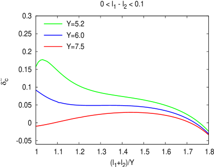
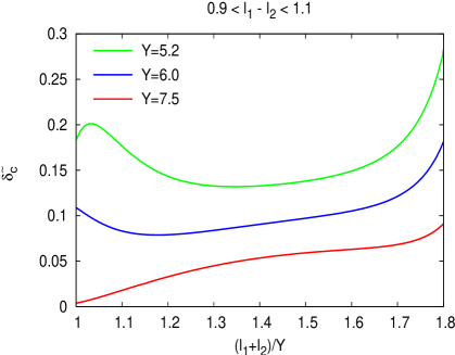
We have replaced in the denominator of (105) $\tilde{\Delta}$ with $\Delta$, which amounts to neglecting ${\cal O}(\gamma_{0}^{2})$ corrections, because the coefficient of $\gamma_{0}^{-2}(\tilde{\Delta}-\Delta)$ is numerically very small; this occurs for two combined reasons: it is proportional to $(a-3/4)$ which is small, and the combination $(\psi_{1,\ell\,y}\psi_{2,\ell}+\psi_{2,\ell,\ell}\psi_{1,y}+\psi_{2,\ell\,y}\psi_{1,\ell}+\psi_{1,\ell\,\ell}\psi_{2,y})$ that appears in (131) is very small (see Fig. 13). Accordingly,

$$\Upsilon_{q}\stackrel{{\scriptstyle DLA}}{{=}}\ln\Bigg{[}1+\frac{N_{c}}{C_{F}}\displaystyle\frac{1}{1+\Delta}\Bigg{]}.$$

We can use this simplified expression for the MLLA reduction of (91).

6.3 The role of corrections; summary of appendix E

Analysis have been done separately for a gluon and a quark jet; their conclusions are very similar.

That $\psi_{\ell}$ and $\psi_{y}$, which are ${\cal O}(\gamma_{0})$ should not exceed reasonable values (fixed arbitrarily to $1$) provides an interval of reliability of our calculations; for example, at LEP-I

$$2.5\leq\ell\leq 4.5\ \text{or}\ 5\leq\ell_{1}+\ell_{2}\leq 9,\quad Y=5.2.$$ (106)

This interval is shifted upwards and gets larger when $Y$ increases.

$\Upsilon_{g}$ and $\Upsilon_{q}$ defined in (104) and (105) and their derivatives are shown to behave smoothly in the confidence interval (106).

The roles of all corrections $\delta_{1},\delta_{2},\Delta$ for a gluon jet, $\tilde{\delta}_{1},\tilde{\delta}_{2},\tilde{\Delta}$ for a quark jet, have been investigated individually. They stay under control in (106). While, in its center, their relative values coincide with what is expected from subsection 4.2, NMLLA corrections can become larger than MLLA close to the bounds; this could make our approximations questionable. Two cases may occur which depend on NMLLA corrections not included in the present frame of calculation; either they largely cancel with the included ones and the sum of all NMLLA corrections is (much) smaller than those of MLLA: then pQCD is trustable at $Y=5.2$; or they do not, the confidence in our results at this energy is weak, despite the fast convergence of the iterative procedure which occurs thanks to the “accidental” observed cancellation between MLLA and those of NMLLA which are included. The steepest descent method [10][11], in which a better control is obtained of MLLA corrections alone, will shed some more light on this question. The global role of all corrections in the iterative process does not exceed $30\%$ for $Y=5.2$ (OPAL) at the bounds of (106); it is generally much smaller, though never negligible. In particular, $\delta_{1}+\delta_{2}+a\Upsilon_{g,\ell}$ for gluons (or $\tilde{\delta}_{1}+\tilde{\delta}_{2}$ for quarks) sum up to ${\cal O}(10^{-2})$ at LEP energy scale (they reach their maximum ${\cal O}(10^{-1})$ at the bound of the interval corresponding to the $30\%$ evoked above).

The role of corrections decreases when the total energy $Y$ of the jet increases, which makes our calculations all the more reliable.

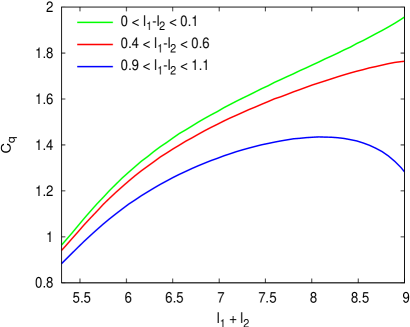
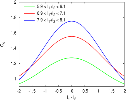
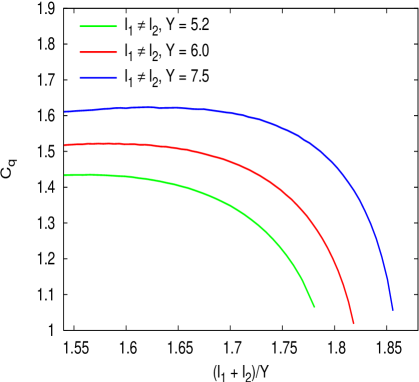
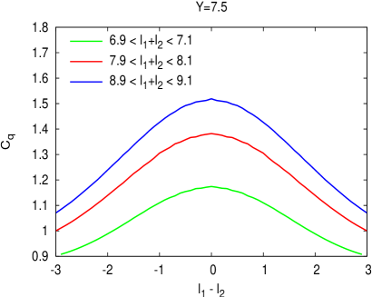
6.4 Results for LEP-I

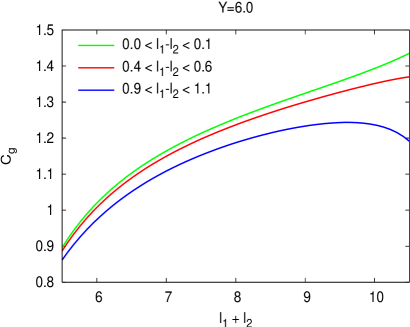
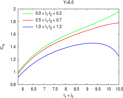
In $e^{+}e^{-}\rightarrow q\bar{q}$ collisions at the $Z^{0}$ peak, $Q=91.2\,\text{GeV}$, $Y=5.2$, and $\gamma_{0}\simeq 0.5$. In Fig. 2 we give the results for gluon jets and in Fig. 3 for quark jets.

Figure 2: ${\cal C}_{g}$ for the LEP-I ($Y=7.5$) inside a gluon jet as function of $\ell_{1}+\ell_{2}$ (left) and of $\ell_{1}-\ell_{2}$ (right)

Figure 3: ${\cal C}_{q}$ for the LEP-I ($Y=7.5$) inside a quark jet as function of $\ell_{1}+\ell_{2}$ (left) and of $\ell_{1}-\ell_{2}$ (right)

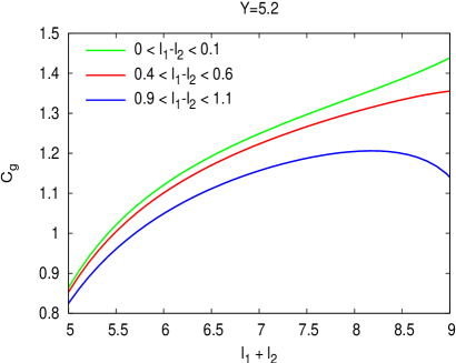
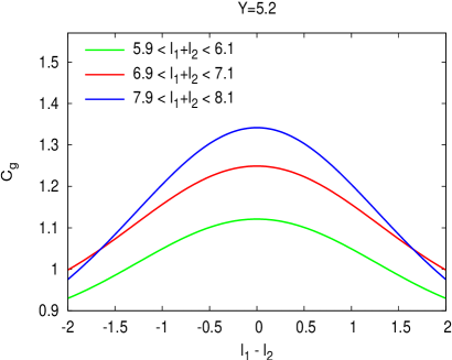
6.4.1 Comments

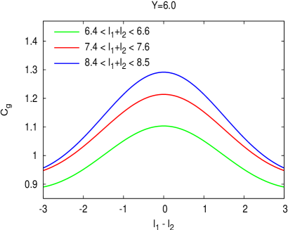
Near the maximum of the single inclusive distribution ($\ell_{1}\approx\ell_{2}\approx\frac{Y}{2}(1+a\gamma_{0})$) our curves are linear functions of $(\ell_{1}+\ell_{2})$ and quadratic functions of $(\ell_{1}-\ell_{2})$, in agreement with the Fong-Webber analysis [6].

$({\cal C}_{q}-1)$ is roughly twice $({\cal C}_{g}-1)$ since gluons cascade twice more than quarks ($\frac{N_{c}}{C_{F}}\approx 2$). The difference is clearly observed from Fig. 2 and Fig. 3 (left) near the hump of the single inclusive distribution ($\ell_{1}+\ell_{2}\simeq 7.6$), that is where most of the partonic multiplication takes place.

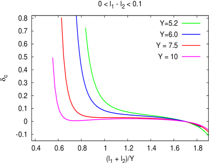
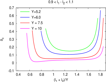
In both cases, $\cal C$ reaches its largest value for $\ell_{1}\approx\ell_{2}$ and steadily increases as a function of $(\ell_{1}+\ell_{2})$ (Fig. 2, left); for $\ell_{1}\neq\ell_{2}$, it increases with $(\ell_{1}+\ell_{2})$, then flattens off and decreases.

Both ${\cal C}$’s decrease as $|\ell_{1}-\ell_{2}|$ becomes large (Fig. 2 and 3, right). The quark’s tail is steeper than the gluon’s; for $5.9<\ell_{1}+\ell_{2}<6.1$, $({\cal C}-1)$ becomes negative when $\ell_{1}-\ell_{2}$ increases; ${\cal C}\geq 1$ as soon as $\ell_{1},\ell_{2}\geq 2.75\,(x_{1},x_{2}\leq 0.06)$; this bounds is close to $\ell\geq 2.4$ found in subsection 4.5 or $\ell\geq 2.5$ of (181).

One finds the limit

$${\cal C}_{g\,or\,q}\stackrel{{\scriptstyle\ell_{1}+\ell_{2}\to 2Y}}{{\longrightarrow}}1.$$ (107)

Figure 4: Decrease of the correlation for $\ell_{1}\neq\ell_{2}$ at $Y=5.2$, $Y=6.0$ and $Y=7.5$

Actually, one observes on Figs. 2, 3 and 4 that a stronger statement holds. Namely, when we take the limit $\ell_{2}\to Y$ for the softer particle, the correlator goes to $1$. This is the consequence of QCD coherence. The softer gluon is emitted at larger angles by the total color charge of the jet and thus becomes de-correlated with the internal partonic structure of the jet.

The same phenomenon explains the flattening and the decrease of ${\cal C}$’s at $\ell_{1}\neq\ell_{2}$.

An interesting phenomenon is the seemingly continuous increase of ${\cal C}_{g}$ and ${\cal C}_{q}$ at large $Y$ for $\ell_{1}\approx\ell_{2}$ (green curves in figs. 2 and 3 left). Like we discussed in [12] concerning inclusive distributions, here we reach a domain where a perturbative analysis cannot be trusted because of the divergence of $\alpha_{s}$. Indeed, when $(\ell_{1}+\ell_{2})$ gets close to its limiting kinematical value ($2Y$), both $y_{1}$ and $y_{2}$ get close to $0$, such that the corresponding $\alpha_{s}(k_{1\perp}^{2})$ and $\alpha_{s}(k_{2\perp}^{2})$ cannot but become out of control. Away from the $\ell_{1}\approx\ell_{2}$ diagonal, taking $\ell_{2}\to Y$ ($y_{2}\to 0$), we have $y_{1}\to\eta>0$ and the emission of the harder parton still stays under control.

The two limitations of our approach already pointed at in [12] are found again here:

$\ast$ $x$ should be small enough such that our soft approximation stays valid;

$\ast$ no running coupling constant should get too large such that pQCD stays reliable.

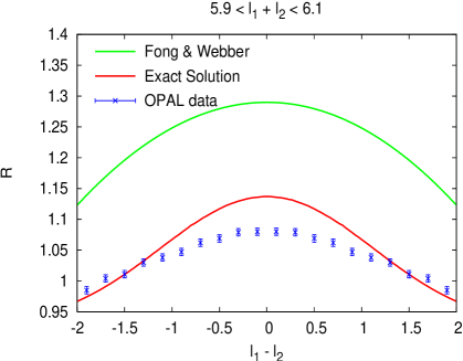
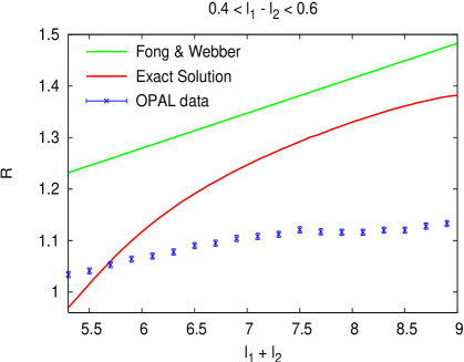
6.5 Comparison with the data from LEP-I

OPAL results are given in terms of

$$R\left(\ell_{1},\ell_{2},Y\right)\>=\>\frac{1}{2}+\frac{1}{2}{\cal C}_{q}\left(\ell_{1},\ell_{2},Y\right).$$

In Fig. 5 we compare our prediction with the OPAL data [7] and the Fong-Webber curves (see subsection 6.6 and [6]).

Figure 5: Correlations $R$ between two particles produced in $e^{+}e^{-}\rightarrow q\bar{q}$ compared with the OPAL data and the Fong-Webber approximation

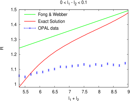
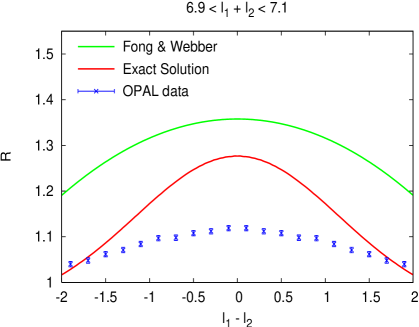
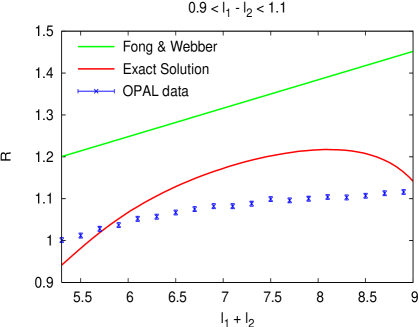
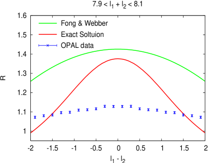
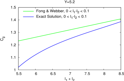
6.6 Comparing with the Fong-Webber approximation

The only pQCD analysis of two-particle correlations in jets beyond DLA was performed by Fong and Webber in 1990. In [6] the next-to-leading ${\cal O}({\gamma_{0}})$ correction, ${\cal C}_{g\,or\,q}=1+\sqrt{\alpha_{s}}+\cdots$, to the normalized two-particle correlator was calculated. This expression was derived in the region $|\ell_{1}-\ell_{2}|/Y\ll 1$, that is when the energies of the registered particles are close to each other (and to the maximum of the inclusive distribution [2][4][13]). In this approximation the correlation function is quadratic in $(\ell_{1}-\ell_{2})$ and increases linearly with $(\ell_{1}+\ell_{2})$, see (109). For example, if one replaces the expression of the single inclusive distribution distorted gaussian [13] (obtained in the region $\ell\approx\frac{Y}{2}(1+a\gamma_{0})$) into (84) the MLLA result for a gluon jet reads

$${\cal C}_{g}(\ell_{1},\ell_{2},Y)\approx 1+\frac{1-\bigg{(}5b-3b\displaystyle{\frac{\ell_{1}+\ell_{2}}{Y}}\bigg{)}\gamma_{0}+{\cal O}(\gamma_{0}^{2})}{3+9\bigg{(}\displaystyle{\frac{\ell_{1}-\ell_{2}}{Y}}\bigg{)}^{2}-\left(2\beta+5a-3a\displaystyle{\frac{\ell_{1}+\ell_{2}}{Y}}\right)\gamma_{0}+{\cal O}(\gamma_{0}^{2})},$$ (108)

where we have neglected the MLLA correction $\delta_{1}\simeq(\ell_{1}-\ell_{2})^{2}\sqrt{\alpha_{s}}\simeq 0$ near the hump of the single inclusive distribution ($\ell_{1}\approx\ell_{2}\approx\frac{Y}{2}(1+a\gamma_{0})$). The Fong-Webber answer is obtained by expanding (108) in $\gamma_{0}$ to get [6]

$${\cal C}_{g}^{(\mbox{\scriptsize FW})}\approx\frac{4}{3}-\left(\frac{\ell_{1}-\ell_{2}}{Y}\right)^{2}+\left[-\frac{5}{3}\left(b-\frac{1}{3}a\right)+\frac{2}{9}\beta+\left(b-\frac{1}{3}a\right)\left(\frac{\ell_{1}+\ell_{2}}{Y}\right)\right]\gamma_{0}+{\cal O}(\gamma_{0}^{2}).$$ (109)

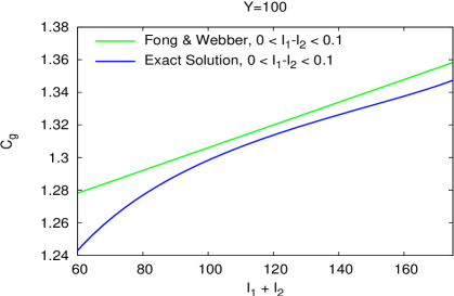
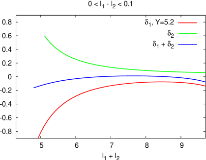
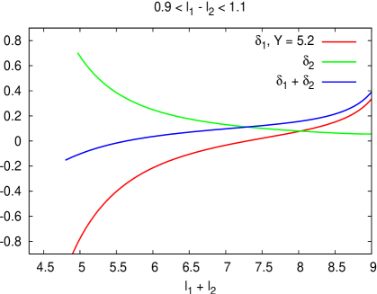
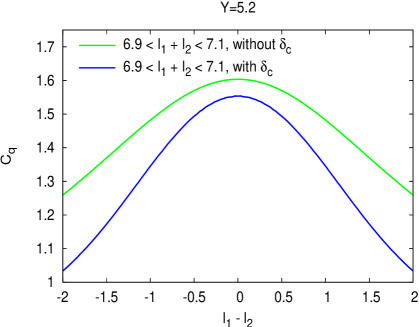
In Fig. 6 we compare, choosing for pedagogical reasons $Y=5.2$ and $Y=100$, our exact solution of the evolution equation with the Fong-Webber predictions [6] for two particle correlations. The mismatch in both cases is, as seen on (109), ${\cal O}(\gamma_{0}^{2})$, and decreases for smaller values of the perturbative expansion parameter $\gamma_{0}$. In particular, at $Y=100$, ($\gamma_{0}^{2}\simeq 0.01$) the exact solution (70) gets close to (109). This comparison is analogous in the case of a quark jet.

We do not perform in the present work such an expansion but keep instead the ratios (70) and (91) as exact solutions of the evolution equations.

Figure 6: Exact ${\cal C}_{g}$ compared with Fong-Webber’s at $Y=5.2$ (left) and $Y=100$ (right)

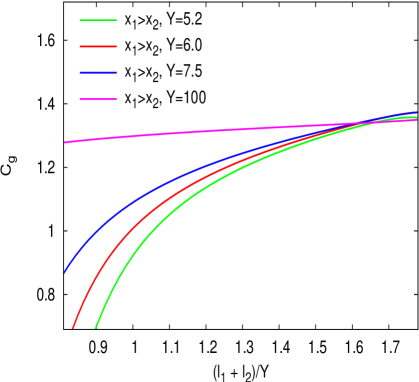
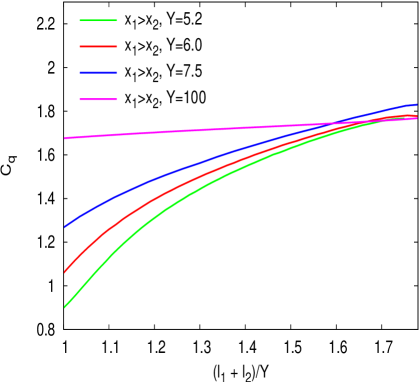
6.7 Predictions for Tevatron and LHC

In hadronic high energy colliders, the nature of the jet (quark or gluon) is not determined, and one simply detects outgoing hadrons, which can originate from either type; one then introduces a “mixing” parameter $\omega$, which is to be determined experimentally, such that, the expression for two particle correlations can be written as a linear combination of ${\cal C}_{g}$ and ${\cal C}_{q}$

$${\cal C}^{mixed}(\omega;\ell_{1},\ell_{2},Y)=A(\omega;\ell_{1},\ell_{2},Y)\,{\cal C}_{q}(\ell_{1},\ell_{2},Y)+B(\omega;\ell_{1},\ell_{2},Y)\,{\cal C}_{g}(\ell_{1},\ell_{2},Y),$$ (110)

where

$$A(\omega;\ell_{1},\ell_{2},Y)=\frac{\omega\,\left[\displaystyle{\frac{Q(\ell_{1},Y)}{G(\ell_{1},Y)}}\displaystyle{\frac{Q(\ell_{2},Y)}{G(\ell_{2},Y)}}\right]}{\bigg{[}1+\omega\bigg{(}\displaystyle{\frac{Q(\ell_{1},Y)}{G(\ell_{1},Y)}}-1\bigg{)}\bigg{]}\bigg{[}1+\omega\bigg{(}\displaystyle{\frac{Q(\ell_{2},Y)}{G(\ell_{2},Y)}}-1\bigg{)}\bigg{]}}$$

and

$$B(\omega;\ell_{1},\ell_{2},Y)=\frac{(1-\omega)}{\bigg{[}1+\omega\bigg{(}\displaystyle{\frac{Q(\ell_{1},Y)}{G(\ell_{1},Y)}}-1\bigg{)}\bigg{]}\bigg{[}1+\omega\bigg{(}\displaystyle{\frac{Q(\ell_{2},Y)}{G(\ell_{2},Y)}}-1\bigg{)}\bigg{]}}.$$

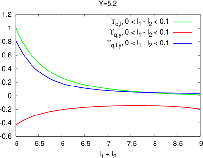
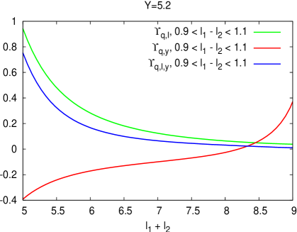
We plug in respectively (70) (91) for ${\cal C}_{g}$ and ${\cal C}_{q}$; the predictions for the latter are given in Figs. 7 and 8 for the Tevatron, Figs. 9 and 10 for the LHC.

Figure 7: ${\cal C}_{g}$ for the Tevatron ($Y=6.0$) as function of $\ell_{1}+\ell_{2}$ (left) and of $\ell_{1}-\ell_{2}$ (right)

Figure 8: ${\cal C}_{q}$ for the Tevatron ($Y=6.0$) as function of $\ell_{1}+\ell_{2}$ (left) and of $\ell_{1}-\ell_{2}$ (right)

Figure 9: ${\cal C}_{g}$ for the LHC ($Y=7.5$) inside a gluon jet as function of $\ell_{1}+\ell_{2}$ (left) and of $\ell_{1}-\ell_{2}$ (right)

Figure 10: ${\cal C}_{q}$ for the LHC ($Y=7.5$) inside a gluon jet as function of $\ell_{1}+\ell_{2}$ (left) and of $\ell_{1}-\ell_{2}$ (right)

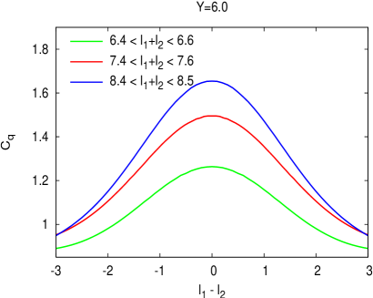
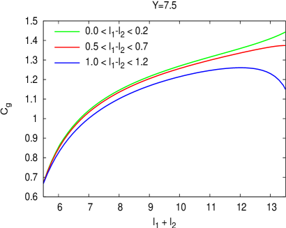
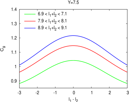
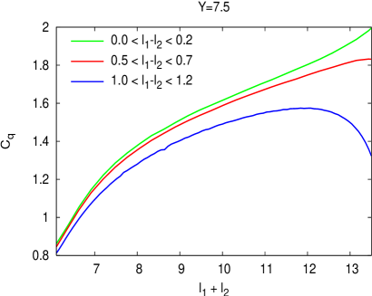
6.7.1 Comments

For both $Y=6.0$ (Tevatron) and $Y=7.5$ (LHC), the global behavior given in 6.4.1 also holds. The interval corresponding to the condition ${\cal C}_{g\,or\,q}>1$ is shifted toward larger values of $\ell$ (smaller $x$) as compared with the $Y=5.2$ case, in agreement with the predictions of (4.5) and (5.4). Numerically, this is achieved for $\ell>2.9$ ($\ell>3.2$) at $Y=6.0$ ($Y=7.5$) in a gluon jet at the Tevatron (LHC). For a quark jet, these values become respectively $\ell>3.1$ ($\ell>3.3$) and one can check that they are close to the approximated ones obtained in (4.5) and (5.4).

One notices that correlations increase as the total energy (Y) increases (LHC $>$ TeV $>$ LEP-I).

6.8 Asymptotic behavior of $\boldsymbol{{\cal C}_{g\,or\,q}}$

We display in Fig. 11 the asymptotic behavior of ${\cal C}_{g}$ and ${\cal C}_{q}$ when $Y$ increases.

$${\cal C}_{g}\stackrel{{\scriptstyle Y\to\infty}}{{\longrightarrow}}\frac{<n(n-1)>_{g}}{<n>_{g}^{2}}\approx 1+\frac{1}{3}\approx 1.33,\quad{\cal C}_{q}\stackrel{{\scriptstyle Y\to\infty}}{{\longrightarrow}}\frac{<n(n-1)>_{q}}{<n>_{q}^{2}}\approx 1+\frac{1}{3}\frac{N_{c}}{C_{F}}=1.75,$$

where $n$ is the multiplicity inside one jet. These limits coincide with those of the DLA multiplicity correlator [14][15]. It confirms the consistency of our approach.

Figure 11: Asymptotic behavior of ${\cal C}_{g}$ and ${\cal C}_{q}$ when $Y$ increases

7 CONCLUSION

In this paper two particle correlations between soft partons in quark and gluon jets were considered.

Corresponding evolution equations for parton correlators were derived in the next to leading approximation of perturbative QCD, known as MLLA, which accounts for QCD coherence (angular ordering) on soft gluon multiplication, hard corrections to parton splittings and the running coupling effects.

The MLLA equations for correlators were analyzed and solved iteratively. This allowed us to generalize the result previously obtained by Fong and Webber in [6] that was valid in the vicinity of the maximum of the single inclusive parton energy distribution (”hump”).

In particular, we have analyzed the regions of moderately small $x$ above which the correlation becomes ”negative” (${\cal C}-1<0$). This happens when suppression because of the limitation of the phase space takes over the positive correlation due to gluon cascading.

Also, the correlation vanishes (${\cal C}\to 1$) when one of the partons becomes very soft ($\ell=\ln 1/x\to Y=\ln E\Theta/Q_{0}$). The reason for that is dynamical rather than kinematical: radiation of a soft gluon occurs at large angles which makes the radiation coherent and thus insensitive to the internal parton structure of the jet ensemble.

Qualitatively, our MLLA result agrees better with available OPAL data than the Fong–Webber prediction. There remains however a significant discrepancy, markedly at very small $x$. In this region non-perturbative effects are likely to be more pronounced. They may undermine the applicability to particle correlations of the local parton–hadron duality considerations that were successful in translating parton level predictions to hadronic observations in the case of more inclusive single particle energy spectra.

Forthcoming data from Tevatron as well as future studies at LHC should help to elucidate the problem.

Acknowledgments: It is a great pleasure to thank Yuri Dokshitzer and Bruno Machet for their guidance and encouragements. I thank François Arléo, Bruno Durin for many discussions and Gavin Salam for his expert help in numerical calculations.

Appendix A DERIVATION OF THE GLUON CORRELATOR $\boldsymbol{{\cal C}_{g}}$ IN (70)

One differentiates $G^{(2)}-G_{1}G_{2}\equiv G_{1}G_{2}\big{(}{\cal C}_{g}-1\big{)}$ with respect to $\ell_{1}$ and $y_{2}$ and use the evolution equations (44) and (67).

By explicit differentiation and using the definitions (refeq:nota4bis)-(76) one gets

$$\Big{[}G_{1}G_{2}\big{(}{\cal C}_{g}-1\big{)}\Big{]}_{\ell\,y}\!\! \!\!=\!\! \!\!G_{1}G_{2}\Big{[}{\cal C}_{g,\ell\,y}+{\cal C}_{g,\ell}\big{(}\psi_{1,y}+\psi_{2,y}\big{)}+{\cal C}_{g,y}\big{(}\psi_{1,\ell}+\psi_{2,\ell}\big{)}\Big{]}$$ (111)

$$\!\!+\!\! \!\!({\cal C}_{g}-1)\Big{[}G_{1}G_{2}\big{(}\psi_{1,\ell}\psi_{2,y}+\psi_{2,\ell}\psi_{1,y}\big{)}+G_{1}G_{2,\ell\,y}+G_{2}G_{1,\ell\,y}\Big{]};$$ (112)

the definition (71) of $\chi$ entails ${\cal C}_{g,\ell}=\chi_{\ell}{\cal C}_{g}$, ${\cal C}_{g,y}=\chi_{y}{\cal C}_{g}$, ${\cal C}_{g,\ell\,y}={\cal C}_{g}\big{(}\chi_{\ell\,y}+\chi_{\ell}\chi_{y}\big{)}$, such that (112) rewrites

$$\Big{[}G^{(2)}-G_{1}G_{2}\Big{]}_{\ell\,y}\!\! \!\!=\!\! \!\!{\cal C}_{g}\;G_{1}G_{2}\Big{[}\big{(}\chi_{\ell\,y}+\chi_{\ell}\chi_{y}\big{)}+\chi_{\ell}\big{(}\psi_{1,y}+\psi_{2,y}\big{)}+\chi_{y}\big{(}\psi_{1,\ell}+\psi_{2,\ell}\big{)}\Big{]}$$ (113)

$$\!\!+\!\! \!\!({\cal C}_{g}-1)\Big{[}G_{1}G_{2}\big{(}\psi_{1,\ell}\psi_{2,y}+\psi_{1,y}\psi_{2,\ell}\big{)}+G_{1}G_{2,\ell\,y}+G_{2}G_{1,\ell\,y}\Big{]}.$$ (114)

By differentiating the evolution equation for the inclusive spectra (44) with respect to $y$ and $\ell$ one gets

$$G_{k,\ell\,y}=\gamma_{0}^{2}\Big{(}1-a\big{(}\psi_{k,\ell}-{\beta}\gamma_{0}^{2}\big{)}\Big{)}G_{k},$$ (115)

where one has used the definition (72)(73) of $\psi_{k,\ell}$ to replace $\frac{dG_{k}}{d\ell}$ with $G_{k}\psi_{k,\ell}$, and (46) to evaluate $\frac{d}{d\ell}\gamma_{0}^{2}=-\beta\gamma_{0}^{4}$. Substituting into (114) yields

$$\frac{l.h.s.(\ref{eq:eveeqglu})\big{|}_{\ell\,y}}{\gamma_{0}^{2}G_{1}G_{2}}=({\cal C}_{g}-1)\bigg{(}2-a\left(\psi_{1,\ell}+\psi_{2,\ell}\right)+\frac{\psi_{1,\ell}\psi_{2,y}+\psi_{1,y}\psi_{2,\ell}}{\gamma_{0}^{2}}+2a{\beta}\gamma_{0}^{2}\bigg{)}+{\cal C}_{g}\big{(}\delta_{1}+\delta_{2}\big{)},$$ (116)

where $\delta_{1}$ and $\delta_{2}$ are defined in (75) (76).

Differentiating now the r.h.s. of (67) with respect to $y_{2}$ and $\ell_{1}$, one gets

$$\frac{r.h.s.(\ref{eq:eveeqglu})\Big{|}_{\ell\,y}}{\gamma_{0}^{2}\,G_{1}G_{2}}={\cal C}_{g}\big{(}1-a\left(\psi_{1,\ell}+\psi_{2,\ell}-{\beta}\gamma_{0}^{2}\right)\Big{)}-{\cal C}_{g}a\chi_{\ell}+(a-b)\left(\psi_{1,\ell}+\psi_{2,\ell}-{\beta}\gamma_{0}^{2}\right).$$ (117)

Equating the expressions (116) and (117) for the correlation function we derive

$$({\cal C}_{g}-1)\Big{(}1+\Delta+\delta_{1}+a\left(\chi_{\ell}+{\beta\gamma_{0}^{2}}\right)+\delta_{2}\Big{)}=1-b\big{(}\psi_{1,\ell}+\psi_{2,\ell}-\beta\gamma_{0}^{2}\big{)}-\delta_{1}-(a\chi_{\ell}+\delta_{2}),$$ (118)

which gives (70).

Appendix B DERIVATION OF THE QUARK CORRELATOR $\boldsymbol{{\cal C}_{q}}$ IN (91)

B.1 Derivation of (91)

The method is the same as in appendix A: one evaluates now $\big{[}Q^{(2)}-{Q_{1}}{Q_{2}}\big{]}_{\ell\,y}\equiv\Big{[}{\cal C}_{q}-1)Q_{1}Q_{2}\Big{]}_{\ell\,y}$.

First, by differentiating the evolution equation (66), one gets

$$\big{[}Q^{(2)}-{Q_{1}}{Q_{2}}\big{]}_{\ell\,y}=\frac{C_{F}}{N_{c}}\gamma_{0}^{2}{\cal C}_{g}G_{1}G_{2}\Big{(}1-\frac{3}{4}\big{(}\psi_{1,\ell}+\psi_{2,\ell}+\chi_{\ell}-\beta\gamma_{0}^{2}\big{)}\Big{)};$$ (119)

then, one explicitly differentiates $\Big{[}({\cal C}_{q}-1)Q_{1}Q_{2}\Big{]}$ and makes use of

$$Q_{k,\ell\,y}=\frac{C_{F}}{N_{c}}\gamma_{0}^{2}G_{k}\Big{(}1-\frac{3}{4}(\psi_{k,\ell}-\beta\gamma_{0}^{2})\Big{)},$$ (120)

which comes directly from differentiating the r.h.s of (43) with respect to $\ell$ and $y$; this yields

$$\big{[}Q^{(2)}-{Q_{1}}{Q_{2}}\big{]}_{\ell\,y}\!\! \!\!=\!\! \!\!{\cal C}_{q}Q_{1}Q_{2}\Big{[}\sigma_{\ell}\big{(}\varphi_{1,y}+\varphi_{2,y}\big{)}+\sigma_{\ell}\big{(}\varphi_{1,\ell}+\varphi_{2,\ell}\big{)}+\sigma_{\ell\,y}+\sigma_{\ell}\sigma_{y}\Big{]}$$ (123)

$$+\big{(}{\cal C}_{q}-1\big{)}Q_{1}Q_{2}\gamma_{0}^{2}\Big{[}\varphi_{1,\ell}\varphi_{2,y}+\varphi_{1,y}\varphi_{2,\ell}\Big{]}$$

$$\hskip-56.9055pt+\big{(}{\cal C}_{q}-1\big{)}\gamma_{0}^{2}\frac{C_{F}}{N_{c}}\Big{[}\big{(}G_{1}Q_{2}+Q_{1}G_{2}\big{)}-\frac{3}{4}G_{1}Q_{2}\big{(}\psi_{1,\ell}-\beta\gamma_{0}^{2}\big{)}-\frac{3}{4}Q_{1}G_{2}\big{(}\psi_{2,\ell}-\beta\gamma_{0}^{2}\big{)}\Big{]};$$

equating (119) and (LABEL:eq:explidif) gives

$${\cal C}_{q}-1=\frac{\frac{N_{c}}{C_{F}}{\cal C}_{g}\bigg{[}1-\frac{3}{4}\Big{(}\psi_{1,\ell}+\psi_{2,\ell}+\chi_{\ell}-\beta\gamma_{0}^{2}\Big{)}\bigg{]}\frac{C_{F}}{N_{c}}\frac{G_{1}}{Q_{1}}\frac{C_{F}}{N_{c}}\frac{G_{2}}{Q_{2}}-{\cal C}_{q}\big{(}\tilde{\delta}_{1}+\tilde{\delta}_{2}\big{)}}{\widetilde{\Delta}+\Big{[}1-\frac{3}{4}\big{(}\psi_{1,\ell}-\beta\gamma_{0}^{2}\big{)}\Big{]}\frac{C_{F}}{N_{c}}\frac{G_{1}}{Q_{1}}+\Big{[}1-\frac{3}{4}\big{(}\psi_{2,\ell}-\beta\gamma_{0}^{2}\big{)}\Big{]}\frac{C_{F}}{N_{c}}\frac{G_{2}}{Q_{2}}},$$ (125)

which leads (91).

B.2 Expressing $\boldsymbol{\widetilde{\Delta}}$, $\boldsymbol{\tilde{\delta}_{1}}$ and $\boldsymbol{\tilde{\delta}_{2}}$ in terms of gluon-related quantities

All the intricacies of (125) lie in $\widetilde{\Delta}$, $\tilde{\delta}_{1}$ and $\tilde{\delta}_{2}$ defined in (94), which involve the quark related quantities $\sigma$ and $\varphi$ (95). In what follows, we will express them in terms of the gluon related quantities $\chi$ and $\psi$ (71)(72)(73).

B.2.1 Expression for $\boldsymbol{\tilde{\Delta}}$

Differentiating (47) with respect to $\ell$ yields

$$Q_{k,\ell}=\frac{C_{F}}{N_{c}}G_{k,\ell}\bigg{[}1+\Big{(}a-\frac{3}{4}\Big{)}\psi_{k,\ell}\bigg{]}+\frac{C_{F}}{N_{c}}G_{k}\bigg{(}a-\frac{3}{4}\bigg{)}\psi_{k,\ell\,\ell}+{\cal O}(\gamma_{0}^{4});$$ (126)

then

$$\varphi_{\ell}=\frac{Q_{k,\ell}}{Q_{k}}=\left\{\frac{C_{F}}{N_{c}}G_{k,\ell}\Big{[}1+\Big{(}a-\frac{3}{4}\Big{)}\psi_{k,\ell}\Big{]}+\frac{C_{F}}{N_{c}}G_{k}\Big{(}a-\frac{3}{4}\Big{)}\psi_{k,\ell\,\ell}\right\}\Big{[}G_{k}^{-1}-\Big{(}a-\frac{3}{4}\Big{)}\psi_{k,\ell}G_{k}^{-1}\Big{]}$$ (127)

yields

$$\varphi_{k,\ell}=\psi_{k,\ell}+\Big{(}a-\frac{3}{4}\Big{)}\psi_{k,\ell\,\ell}+{\cal O}(\gamma_{0}^{4}).$$ (128)

Differentiating (47) with respect to $y$ yields

$$Q_{k,y}=\frac{C_{F}}{N_{c}}G_{k,y}\bigg{[}1+\Big{(}a-\frac{3}{4}\Big{)}\psi_{k,\ell}\bigg{]}+\frac{C_{F}}{N_{c}}G_{k}\bigg{(}a-\frac{3}{4}\bigg{)}\psi_{k,\ell\,y}+{\cal O}(\gamma_{0}^{4}),$$ (129)

and, finally,

$$\varphi_{k,y}=\psi_{k,y}+\Big{(}a-\frac{3}{4}\Big{)}\psi_{k,\ell\,y}+{\cal O}(\gamma_{0}^{4}).$$ (130)

Using (128) and (130) in $\widetilde{\Delta}$ given by (94) gives

$$\widetilde{\Delta}\approx\Delta+\Big{(}a-\frac{3}{4}\Big{)}\Big{(}\psi_{1,\ell\,y}\psi_{2,\ell}+\psi_{2,\ell\,\ell}\psi_{1,y}+\psi_{2,\ell\,y}\psi_{1,\ell}+\psi_{1,\ell\,\ell}\psi_{2,y}\Big{)}\gamma_{0}^{-2},$$ (131)

which shows in particular, that $\widetilde{\Delta}\approx\Delta+{\cal O}(\gamma_{0}^{2})$.

B.2.2 Expression for $\boldsymbol{\tilde{\delta}_{1},\tilde{\delta}_{2}}$

(94) entails ${\cal C}_{q}\gamma_{0}^{2}\tilde{\delta}_{1}={\cal C}_{q,\ell}\big{(}\varphi_{1,y}+\varphi_{2,y}\big{)}+{\cal C}_{q,y}\big{(}\varphi_{1,\ell}+\varphi_{2,\ell}\big{)}$; since ${\cal C}_{q,\ell}$ and ${\cal C}_{q,y}$ are ${\cal O}(\gamma_{0}^{2})$ and considering (130) and (128), we can approximate

$${\cal C}_{q}\gamma_{0}^{2}\tilde{\delta}_{1}={\cal C}_{q,\ell}\big{(}\psi_{1,y}+\psi_{2,y}\big{)}+{\cal C}_{q,y}\big{(}\psi_{1,\ell}+\psi_{2,\ell}\big{)}+{\cal O}(\gamma_{0}^{5}),$$ (132)

which needs evaluating ${\cal C}_{q,\ell}$ and ${\cal C}_{q,y}$ in terms of gluonic quantities. Actually, since ${\cal C}_{q}\tilde{\delta}_{1}$ and ${\cal C}_{q}\tilde{\delta}_{2}$ occur as MLLA and NMLLA corrections in (125), it is enough to take the leading (DLA) term of ${\cal C}_{q}$ to estimate them

$${\cal C}_{q}^{DLA}=1+\frac{N_{c}}{C_{F}}\frac{1}{1+\Delta}=1-\frac{N_{c}}{C_{F}}+\frac{N_{c}}{C_{F}}\Big{(}1+\frac{1}{1+\Delta}\Big{)};$$ (133)

differentiating then over $\ell$ and $y$ yields

$${\cal C}_{q,\ell}^{DLA} = -\frac{N_{c}}{C_{F}}\frac{\Delta_{\ell}}{\Big{(}1+\Delta\Big{)}^{2}}=\frac{N_{c}}{C_{F}}{\cal C}_{g,\ell}^{DLA},$$ (134)

$${\cal C}_{q,y}^{DLA} = -\frac{N_{c}}{C_{F}}\frac{\Delta_{y}}{\Big{(}1+\Delta\Big{)}^{2}}=\frac{N_{c}}{C_{F}}{\cal C}_{g,y}^{DLA}.$$ (135)

Substituting (134), (135) into (132) one gets

$${\cal C}_{q}\tilde{\delta}_{1}={\cal C}_{g}\delta_{1}+{\cal{O}}(\gamma_{0}^{3}).$$ (136)

Likewise, calculating $\gamma_{0}^{2}{\cal C}_{q}\tilde{\delta}_{2}$ needs evaluating ${\cal C}_{q,\ell\,y}^{DLA}$ in terms of gluonic quantities. Using (134) one gets

$${\cal C}_{q}\tilde{\delta}_{2}={\cal C}_{g}\delta_{2}+{\cal{O}}(\gamma_{0}^{4}).$$ (137)

Accordingly, ${\cal C}_{q}(\tilde{\delta}_{1}+\tilde{\delta}_{2})$ can be replaced by ${\cal C}_{g}(\delta_{1}+\delta_{2})$ to get the solution (125). This approximation is used to get the MLLA solution (100) of (125).

Appendix C DLA INSPIRED SOLUTION OF THE MLLA EVOLUTION EQUATIONS FOR THE INCLUSIVE SPECTRUM

This appendix completes subsection 4.2. For pedagogical reasons we will estimate the solution of (44) when neglecting the running of $\alpha_{s}$ (constant-$\gamma_{0}^{2}$) (see [2][4] and references therein). We perform a Mellin’s transformation of $G(\ell,y)$

$$G\left(\ell,y\right)=\iint_{C}\frac{d\omega\,d\nu}{\left(2\pi i\right)^{2}}\,e^{\omega\ell}\,e^{\nu y}\,{\cal G}\left(\omega,\nu\right).$$ (138)

The contour C lies to the right of all singularities. In (44) one set the lower bounds for $\ell$ and $y$ to $-\infty$ since these integrals are vanishing when one closes the C-contour to the right. Using the Mellin’s representation for $\delta(\ell)$

$$\delta(\ell)=\iint_{C}\frac{d\omega d\nu}{\left(2\pi i\right)^{2}}\,e^{\omega\ell}\,e^{\nu y}\frac{1}{\nu},$$ (139)

one gets

$${\cal{G}}\left(\omega,\nu\right)=\displaystyle{\frac{1}{\nu-\gamma_{0}^{2}\big{(}1/\omega-a\big{)}}}.$$ (140)

Substituting (140) into (138) and extracting the pole ($\nu_{0}=\gamma_{0}^{2}\big{(}1/\omega-a\big{)}$) from the denominator of (140) one gets rid of the integration over $\nu$ and obtains the following representation

$$G\left(\ell,y\right)=\int_{C}\frac{d\omega}{2\pi i}\exp{\Big{[}\omega\ell+\gamma_{0}^{2}\big{(}1/\omega-a\big{)}y\Big{]}};$$ (141)

finally treating $\ell$ as a large variable (soft approximation $x\ll 1$) allows us to have an estimate of (141) by performing the steepest descent method; one then has

$$G(\ell,y)\stackrel{{\scriptstyle x\ll 1}}{{\approx}}\frac{1}{2}\sqrt{\frac{\gamma_{0}\,y^{1/2}}{{\pi\,\ell^{3/2}}}}\exp{\left(2\gamma_{0}\sqrt{\ell\,y}-a\gamma_{0}^{2}\,y\right)}.$$ (142)

However, since we are interested in getting logarithmic derivatives; in this approximation we can drop the normalization factor of (142) which leads to sub-leading corrections that we do not take into account here; we can use instead

$$G(\ell,y)\stackrel{{\scriptstyle x\ll 1}}{{\simeq}}\exp{\left(2\gamma_{0}\sqrt{\ell\,y}-a\gamma_{0}^{2}\,y\right)},$$ (143)

which is (78).

Appendix D EXACT SOLUTION OF THE MLLA EVOLUTION EQUATION FOR THE INCLUSIVE SPECTRUM

We solve (44) by performing a Mellin’s transformation of the following function ($\gamma_{0}^{2}$ , $\beta$ and $\lambda$ are defined in (46), (7)):

$$F\left(\ell,y\right)=\gamma_{0}^{2}(\ell+y)G\left(\ell,y\right),$$

that is,

$$F\left(\ell,y\right)=\iint_{C}\frac{d\omega d\nu}{\left(2\pi i\right)^{2}}\,e^{\omega\ell}\,e^{\nu y}\,{\cal F}\left(\omega,\nu\right).$$ (144)

Substituting (144) into (44) we obtain:

$${\beta}\left(\ell+y+\lambda\right)\iint\frac{d\omega d\nu}{\left(2\pi i\right)^{2}}\,e^{\omega\ell}\,e^{\nu y}\,{\cal F}\left(\omega,\nu\right)\!\! \!\!=\!\! \!\!\iint\frac{d\omega d\nu}{\left(2\pi i\right)^{2}}\,e^{\omega\ell}\,e^{\nu y}\left[\frac{1}{\nu}+\frac{{\cal F}\left(\omega,\nu\right)}{\omega\nu}\right]$$

$$\!\!-\!\! \!\!a\!\!\iint\frac{d\omega d\nu}{\left(2\pi i\right)^{2}}\,e^{\omega\ell}\,e^{\nu y}\frac{{\cal F}(\omega,\nu)}{\nu},$$

where we have again replaced $\delta(\ell)$ by its Mellin’s representation (139). Then using the equivalence $\ell\leftrightarrow\frac{\partial}{\partial\omega},\,y\leftrightarrow\frac{\partial}{\partial\nu}$, we integrate the l.h.s. by parts and obtain:

$$\beta\!\!\iint\frac{d\omega d\nu}{\left(2\pi i\right)^{2}}\left[\left(\frac{\partial}{\partial\omega}\!+\!\frac{\partial}{\partial\nu}\!+\!\lambda\right)e^{\omega\ell+\nu y}\right]{\cal F}\left(\omega,\nu\right)=\beta\!\!\iint\frac{d\omega d\nu}{\left(2\pi i\right)^{2}}\left(\lambda{\cal F}\!-\!\frac{\partial{\cal F}}{\partial\omega}\!-\!\frac{\partial{\cal F}}{\partial\nu}\right)\,e^{\omega\ell+\nu y}.$$

We are finally left with the following inhomogeneous differential equation:

$$\beta\left(\lambda{\cal F}\!-\!\frac{\partial{\cal F}}{\partial\omega}\!-\!\frac{\partial{\cal F}}{\partial\nu}\right)=\frac{1}{\nu}\!+\!\frac{{\cal F}}{\omega\nu}-a\frac{{\cal F}}{\nu}.$$ (145)

The variables $\omega$ and $\nu$ can be changed conveniently to

$$\omega^{\prime}=\frac{\omega+\nu}{2},\qquad\nu^{\prime}=\frac{\omega-\nu}{2},$$

such that (145) is now decoupled and can be easily solved:

$$\beta\left(\lambda{\cal F}-\frac{d{\cal F}}{d\omega^{\prime}}\right)=\frac{1}{\omega^{\prime}-\nu^{\prime}}+\frac{{\cal F}}{\omega^{\prime 2}-\nu^{\prime 2}}-a\frac{{\cal F}}{\omega^{\prime}-\nu^{\prime}}.$$

The solution of the corresponding homogeneous equation, written as a function of $\omega$ and $\nu$, is the following:

$${\cal F}^{h}\left(\omega,\nu\right)=\frac{1}{\beta}\int_{0}^{\infty}\frac{ds}{\nu+s}\left(\frac{\omega\left(\nu+s\right)}{\left(\omega+s\right)\nu}\right)^{1/\beta\left(\omega-\nu\right)}\left(\frac{\nu}{\nu+s}\right)^{a/\beta}.$$

We finally obtain the exact solution of (44) given by the following Mellin’s representation:

$$G\left(\ell,y\right)=\left(\ell\!+\!y\!+\!\lambda\right)\!\!\iint\frac{d\omega\,d\nu}{\left(2\pi i\right)^{2}}e^{\omega\ell+\nu y}\!\!\int_{0}^{\infty}\frac{ds}{\nu+s}\!\!\left(\frac{\omega\left(\nu+s\right)}{\left(\omega+s\right)\nu}\right)^{1/\beta\left(\omega-\nu\right)}\!\!\left(\frac{\nu}{\nu+s}\right)^{a/\beta}\,e^{-\lambda s}.$$ (146)

(146) will be estimated using the steepest descent method in a forthcoming work that will treat two particles correlations at $Q_{0}\geq\Lambda_{QCD}$ ($\lambda=\ln(Q_{0}/\Lambda_{QCD})\neq 0$) [10][11]. Substituting (146) into (67) one has the Mellin’s representation inside a quark jet

$$Q(\ell,y)\!\!=\!\!(\ell\!+\!y\!+\!\lambda)\!\!\iint\frac{d\omega\,d\nu}{\left(2\pi i\right)^{2}}e^{\omega\ell+\nu y}\left(\frac{\gamma_{0}^{2}}{\omega\nu}-\frac{3}{4}\frac{\gamma_{0}^{2}}{\nu}\right)\!\!\int_{0}^{\infty}\frac{ds}{\nu+s}\!\!\left(\!\frac{\omega\left(\nu+s\right)}{\left(\omega+s\right)\nu}\!\right)^{1/\beta\left(\omega-\nu\right)}\!\!\left(\frac{\nu}{\nu+s}\right)^{a/\beta}\!\!e^{-\lambda s};$$

where $\gamma_{0}^{2}/\omega\nu={\cal O}(1)$ and the second term is the MLLA correction $\gamma_{0}^{2}/\nu={\cal O}(\gamma_{0})$.

D.1 Limiting Spectrum, $\boldsymbol{\lambda=0}$

We set $\lambda=0$ (that is $Q_{0}=\Lambda_{QCD}$) in (146) and change variables as follows

$$\bar{\omega}=\omega-\nu,\quad s+\bar{\omega}t=\bar{\omega}/u,\quad A\equiv A(\bar{\omega})=\frac{1}{\beta\bar{\omega}},\quad B=a/\beta$$

to get ($\ell+y=Y$ is used as a variable)

$$G\left(\ell,Y\right)=\int_{\epsilon_{1}-i\infty}^{\epsilon_{1}+i\infty}\frac{d\bar{\omega}}{2\pi i}x^{-\bar{\omega}}\bar{\omega}Y\int_{\epsilon_{2}-i\infty}^{\epsilon_{2}+i\infty}\frac{dt}{2\pi i}\,e^{\bar{\omega}Yt}\left(\frac{t}{1+t}\right)^{-A}t^{B}\int_{0}^{t^{-1}}\,du\,u^{B-1}\left(1+u\right)^{-A};$$ (147)

the last integral of (147) is the representation of the hypergeometric functions of the second kind (see  [16])

$$\int_{0}^{t^{-1}}\,du\,u^{B-1}\left(1+u\right)^{-A}=\frac{t^{-B}}{B}\,_{2}F_{1}\left(A,B;B+1;-t^{-1}\right);$$

for $\Re B>0$, we also have

$${}_{2}F_{1}\left(a,b;c;x\right)=\sum_{n=0}^{\infty}\frac{\left(a\right)_{n}\left(b\right)_{n}x^{n}}{\left(c\right)_{n}n!},$$

where for example

$$\left(a\right)_{n}=\frac{\Gamma\left(a+n\right)}{\Gamma\left(a\right)}=a\left(a+1\right)...\left(a+n-1\right).$$

Therefore (147) can be rewritten in the form:

$$G\left(\ell,Y\right)=\frac{Y}{B}\int_{\epsilon_{1}-i\infty}^{\epsilon_{1}+i\infty}\frac{d\bar{\omega}}{2\pi i}x^{-\bar{\omega}}\bar{\omega}\int_{\epsilon_{2}-i\infty}^{\epsilon_{2}+i\infty}\frac{dt}{2\pi i}\,e^{\bar{\omega}Yt}\left(\frac{t}{1+t}\right)^{-A}\,_{2}F_{1}\left(A,B;B+1;-t^{-1}\right).$$ (148)

By making use of the identity [17]:

$$\left(1+t^{-1}\right)\,_{2}F_{1}\left(-A+B+1,1;B+1;-t^{-1}\right)=\left(\frac{t}{1+t}\right)^{-A}\,_{2}F_{1}\left(A,B;B+1;-t^{-1}\right),$$

we split (148) into two integrals. The solution of the second one is given by the hypergeometric function of the first kind  [17]:

$$\int_{\epsilon_{2}-i\infty}^{\epsilon_{2}+i\infty}\frac{dt}{2\pi i}\,e^{\bar{\omega}Yt}\,t^{-1}\,_{2}F_{1}\left(-A+B+1,1;B+1;-t^{-1}\right)\!=\!_{1}F_{1}\left(-A+B+1;B+1;-\bar{\omega}Y\right).$$ (149)

Taking the derivative of (149) over $(\bar{\omega}Y)$ we obtain:

$$\int_{\epsilon_{2}-i\infty}^{\epsilon_{2}+i\infty}\frac{dt}{2\pi i}\,e^{\bar{\omega}Yt}\,_{2}F_{1}\left(-A+B+1,1;B+1;-t^{-1}\right)\!=\!-\frac{d}{d\left(-\bar{\omega}Y\right)}\,_{1}F_{1}\left(-A+B+1;B+1;-\bar{\omega}Y\right),$$

where,

$${}_{1}F_{1}\left(a;b;x\right)\equiv\Phi\left(a;b;x\right)=\sum_{n=0}^{\infty}\frac{\left(a\right)_{n}x^{n}}{\left(b\right)_{n}n!}.$$

We finally make use of the identity  [17]:

$${}_{1}F_{1}\left(-A+B+1;B+2;-\bar{\omega}Y\right)\!\! \!\!=\!\! \!\!\frac{B+1}{A}\Big{[}\,_{1}F_{1}\left(-A+B+1;B+1;-\bar{\omega}Y\right)\Big{.}$$

$$\!\!-\!\! \!\!\Big{.}\frac{d}{d\left(-\bar{\omega}Y\right)}\,_{1}F_{1}\left(-A+B+1;B+1;-\bar{\omega}Y\right)\Big{]}$$

to get (${}_{1}F_{1}\equiv\Phi$):

$$G\left(\ell,Y\right)=\frac{Y}{\beta B\left(B+1\right)}\int_{\epsilon-i\infty}^{\epsilon+i\infty}\frac{d\bar{\omega}}{2\pi i}x^{-\bar{\omega}}\Phi\left(-A+B+1,B+2,-\bar{\omega}Y\right);$$ (150)

we can rename $\bar{\omega}\rightarrow\omega$ and set $Y=\ell+y$, which yields

$$G\left(\ell,y\right)\!\! \!\!=\!\! \!\!\frac{\ell+y}{\beta B\left(B+1\right)}\int_{\epsilon-i\infty}^{\epsilon+i\infty}\frac{d{\omega}}{2\pi i}x^{-{\omega}}\Phi\left(-A+B+1,B+2,-{\omega}(\ell+y)\right)$$ (151)

$$\!\!=\!\! \!\!\frac{\ell+y}{\beta B\left(B+1\right)}\int_{\epsilon-i\infty}^{\epsilon+i\infty}\frac{d{\omega}}{2\pi i}e^{-{\omega}y}\Phi\left(A+1,B+2,{\omega}(\ell+y)\right).$$

We thus demonstrated that the integral representation (146) is equivalent to (150) in the limit $\lambda=0$. In this problem all functions are derived using (151), and one fixes the value of $Y=\ln(Q/Q_{0})$ (that is fixing the hardness of the process under consideration), such that each result is presented as a function of the energy fraction in the logarithmic scale $\ell=\ln(1/x)$. As demonstrated in [2] [12], the inclusive spectrum can be obtained using (150) and the result is

$$G(\ell,Y)=2\frac{\Gamma(B)}{\beta}\Re\left(\int_{0}^{\frac{\pi}{2}}\frac{d\tau}{\pi}\,e^{-B\alpha}\ {\cal F}_{B}(\tau,y,\ell)\right),$$ (152)

where the integration is performed with respect to $\tau$ defined by $\displaystyle\alpha=\frac{1}{2}\ln\left(\frac{Y}{\ell}-1\right)+i\tau$,

$${\cal F}_{B}(\tau,\ell,Y)\!\! \!\!=\!\! \!\!\left[\frac{\cosh\alpha-\displaystyle{\left(1-\frac{2\ell}{Y}\right)}\sinh\alpha}{\displaystyle\frac{Y}{\beta}\,\frac{\alpha}{\sinh\alpha}}\right]^{B/2}I_{B}\Big{(}2\sqrt{Z(\tau,\ell,Y)}\Big{)},$$ (153)

$$Z(\tau,\ell,Y)\!\! \!\!=\!\! \!\!\frac{Y}{\beta}\,\frac{\alpha}{\sinh\alpha}\,\left[\cosh\alpha-\left(1-\frac{2\ell}{Y}\right)\sinh\alpha\right];$$ (156)

$I_{B}$ is the modified Bessel function of the first kind.

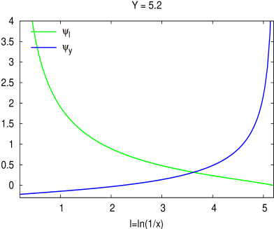
D.2 Logarithmic derivatives of the spectrum, $\boldsymbol{\lambda=0}$

Using the expressions derived in [12] and fixing the sum $\ell+y=Y$, one gets

$$\frac{d}{d\ell}G\left(\ell,Y\right)=2\frac{\Gamma(B)}{\beta}\int_{0}^{\frac{\pi}{2}}\frac{d\tau}{\pi}\,e^{-B\alpha}\left[\frac{1}{Y}\left(1+2e^{\alpha}\sinh{\alpha}\right){\cal{F}}_{B}+\frac{1}{\beta}e^{\alpha}{\cal{F}}_{B+1}\right];$$ (157)

and

$$\frac{d}{dy}G\left(\ell,y\right)\!=\!2\frac{\Gamma(B)}{\beta}\!\int_{0}^{\frac{\pi}{2}}\frac{d\tau}{\pi}\,e^{-B\alpha}\left[\frac{1}{Y}\left(1+2e^{\alpha}\sinh{\alpha}\right){\cal{F}}_{B}+\frac{1}{\beta}e^{\alpha}{\cal{F}}_{B+1}\right.\left.-\frac{2\sinh\alpha}{Y}{\cal{F}}_{B-1}\right].$$ (158)

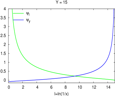
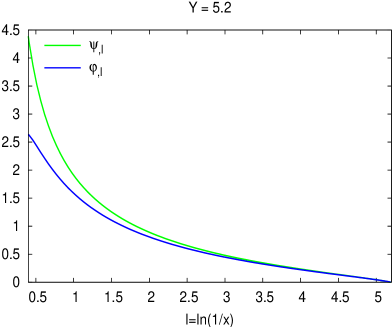
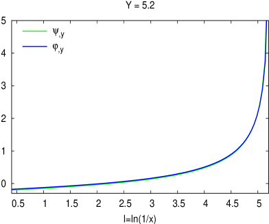
Logarithmic derivatives $\psi_{\ell}$ and $\psi_{y}$ are then constructed according to their definition (72)(73) by dividing (157) and (158) by the inclusive spectrum (152).

Using the expression of Bessel’s series, one gets

$\bullet$ for $\ell\rightarrow 0$;

$$\psi_{\ell} \stackrel{{\scriptstyle\ell\to 0}}{{\simeq}} \frac{a}{\beta\ell}+c_{1}\ln\left(\frac{Y}{\ell}-1\right)\to\infty,$$ (159)

$$c_{1} = \frac{2^{a/\beta+2}}{\pi(a+2\beta)}\int_{0}^{\pi/2}d\tau\,(\cos\tau)^{a/\beta+2}\left[\cos\left(\frac{a}{\beta}\tau\right)-\tan\tau\sin\left(\frac{a}{\beta}\tau\right)\right]=0.4097>0,$$ (160)

$$\psi_{y} \stackrel{{\scriptstyle\ell\to 0}}{{\simeq}} -a\gamma_{0}^{2}+c_{1}\frac{\ell}{y}\to-a\gamma_{0}^{2}.$$ (161)

$\bullet$ for $\ell\rightarrow Y\Leftrightarrow y\rightarrow 0$;

$$\psi_{\ell} \stackrel{{\scriptstyle y\to 0}}{{\simeq}} c_{2}\left(\frac{Y}{\ell}-1\right)\to 0,$$ (162)

$$c_{2} = \frac{2^{a/\beta+2}}{\pi(a+2\beta)}\int_{0}^{\pi/2}d\tau\,(\cos\tau)^{a/\beta+2}\left[\cos\left(\frac{a}{\beta}\tau\right)+\tan\tau\sin\left(\frac{a}{\beta}\tau\right)\right]=0.9218>0;$$ (163)

$$\psi_{y} \stackrel{{\scriptstyle y\to 0}}{{\simeq}} -c_{2}\ln\left(\frac{Y}{\ell}-1\right)\to\infty.$$ (164)

They are represented in Fig. 12 as functions of $\ell$ for two different values of $Y$ ($=5.2,15$).

D.3 Double derivatives

In the core of this paper we also need the expression for $\psi_{,\ell,\ell}$

$$\psi_{\ell\,\ell}=\frac{1}{G}G_{\ell\,\ell}-(\psi_{\ell})^{2}.$$ (165)

By differentiating twice (151) with respect to $\ell$, one gets

$$G_{\ell\,\ell}(\ell,y) \!\!=\!\! \frac{2}{\ell+y}\left(G_{\ell}(\ell,y)-\frac{1}{\ell+y}G(\ell,y)\right)$$ (168)

$$+\frac{(\ell+y)\Gamma(B)}{\beta\Gamma(B+3)}\int_{\epsilon-i\infty}^{\epsilon+i\infty}\frac{d\omega}{2\pi i}e^{-\omega y}\omega^{2}\left(A^{2}+3A+2\right)\Phi\left(A+3,B+4;\omega(\ell+y)\right).$$

Using the procedure of [12] (appendix A.2) and setting $y=Y-\ell$, the result for $G_{\ell\,\ell}$ reads

$$G_{\ell\,\ell}(\ell,Y) \!\!=\!\! \frac{2}{Y}\left(G_{\ell}(\ell,Y)-\frac{1}{Y}G(\ell,Y)\right)$$ (172)

$$+2\frac{\Gamma(B)}{\beta}\int_{0}^{\frac{\pi}{2}}\frac{d\alpha}{\pi}\,e^{-(B-2)\alpha}\left[\frac{1}{\beta^{2}}\,{\cal{F}}_{B+2}+\frac{6}{\beta Y}\sinh\alpha\,{\cal{F}}_{B+1}+\frac{8}{Y^{2}}\sinh^{2}\alpha\,{\cal{F}}_{B}\right].$$

Likewise, for

$$\psi_{y\,y}=\frac{1}{G}G_{y\,y}-(\psi_{y})^{2},$$ (174)

where

$$G_{y\,y}(\ell,y) \!\!=\!\! \gamma_{0}^{2}G(\ell,y)+\frac{1}{Y}\bigg{(}G_{y}(\ell,y)-G_{\ell}(\ell,y)\bigg{)}$$ (177)

$$+\frac{1}{\beta}\frac{(\ell+y)\Gamma(B)}{\Gamma(B+2)}\int_{\epsilon-i\infty}^{\epsilon+i\infty}\frac{d\omega}{2\pi i}e^{-\omega y}\left(\omega^{2}-\frac{\omega}{\beta}\right)\Phi\left(A+1,B+3;\omega(\ell+y)\right),$$

one gets

$$G_{y\,y}(\ell,Y) \!\!=\!\! \gamma_{0}^{2}G(\ell,Y)+\frac{1}{Y}\bigg{(}G_{y}(\ell,Y)-G_{\ell}(\ell,Y)\bigg{)}$$ (180)

$$+4\frac{\Gamma(B)}{\beta}\int_{0}^{\frac{\pi}{2}}\frac{d\alpha}{\pi}\,e^{-(B+1)\alpha}\left[2(B+1)\frac{\sinh^{2}\alpha}{Y^{2}}\,{\cal{F}}_{B-1}-\frac{1}{\beta}\frac{\sinh\alpha}{Y}\,{\cal{F}}_{B}\right].$$

Finally,

$$\psi_{\ell\,y}=\psi_{y\,\ell}=\gamma_{0}^{2}\left[1-a\left(\psi_{\ell}-\beta\gamma_{0}^{2}\right)\right]-\psi_{\ell}\psi_{y}.$$

$\psi_{\ell\,\ell}$, $\psi_{y\,y}$ and $\psi_{\ell\,y}$ are drawn in Fig. 13 of appendix E.1.1 as functions of $\ell$ for fixed $Y$. They are all ${\cal{O}}(\gamma_{0}^{3})$.

Appendix E NUMERICAL ANALYSIS OF CORRECTIONS

In this section, we present plots for the derivatives of $\psi$, and $\varphi$ (see (72)(73) and (95)), for $\Upsilon$ and its derivatives (see (104)(105)), for $\Delta$, $\delta_{1}$, $\delta_{2}$ (see (71)-(76)) and the combination $\delta_{c}\equiv\delta_{1}+\delta_{2}+a\Upsilon_{\ell}$, $\tilde{\delta}_{c}\equiv\tilde{\delta}_{1}+\tilde{\delta}_{2}$.

E.1 Gluon jet

E.1.1 $\boldsymbol{\psi}$ and its derivatives

This subsection is associated with appendices D.2 and D.3 . It enables in particular to visualize the behaviors of $\psi_{\ell}$ and $\psi_{y}$ when $\ell\to 0$ or $y\to 0$, as described in (161) and (164), and to set the $\ell$ interval within which our calculation can be trusted.

Figure 12: Derivatives $\psi_{\ell}$ and $\psi_{y}$ as functions of $\ell$ at fixed $Y=5.2$ (left) and $Y=15$ (right)

Figure 13: Double derivatives $\psi_{\ell\,\ell}$, $\psi_{\ell\,y}$ and $\psi_{y\,y}$ as functions of $\ell$ at fixed $Y$

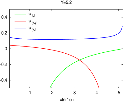
In Fig.12 are drawn $\psi_{\ell}$ and $\psi_{y}$ as functions of $\ell$ for two values $Y=5.2$ corresponding to LEP working conditions, and $Y=15$ corresponding to an unrealistic “high energy limit”.

$\psi_{\ell}$ and ($\psi_{y}$) being both ${\cal{O}}(\gamma_{0})$, they should not exceed a “reasonable value”; setting this value to $1$, $|\psi_{\ell}|<1$ and $|\psi_{y}|<1$ set, for $Y=5.2$, a confidence interval

$$2.5\leq\ell\leq 4.5.$$ (181)

In the high energy limit $Y=15$, this interval becomes, $4.5\leq\ell\leq 13$, in agreement with 4.5.

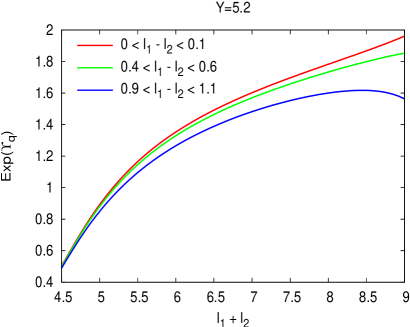
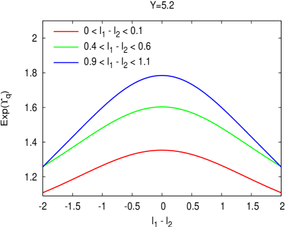
E.1.2 $\boldsymbol{\Delta(\ell_{1},\ell_{2},Y)}$

$\Delta$ has been defined in (74), in which $\psi_{1,\ell}$ and $\psi_{1,y}$ are functions of $\ell_{1}$ and $Y$, $\psi_{2,\ell}$ and $\psi_{2,y}$ are functions of $\ell_{2}$ and $Y$.

Studying the limits $\ell\to 0$ and $\ell\to Y$ of subsection D.2:

• for $\ell_{1},\,\ell_{2}\rightarrow Y$ one gets (using the results of D.2)

  $$\Delta\simeq-c_{2}^{\,2}\left(\frac{Y-\ell_{1}}{\ell_{1}}\ln\frac{Y-\ell_{2}}{\ell_{2}}+\frac{Y-\ell_{2}}{\ell_{2}}\ln\frac{Y-\ell_{1}}{\ell_{1}}\right),$$ (182)

  such that

  $$\Delta\stackrel{{\scriptstyle\ell_{1}-\ell_{2}\to 0}}{{\longrightarrow}}0,\quad\Delta\stackrel{{\scriptstyle\ell_{1}-\ell_{2}\to\infty}}{{\longrightarrow}}+\infty.$$ (183)

• for $\ell_{1},\,\ell_{2}\rightarrow 0$ one gets (according to D.2):

  $$\Delta\simeq-a\gamma_{0}^{2}\left[\frac{a}{\beta}\left(\frac{1}{\ell}_{1}+\frac{1}{\ell}_{2}\right)+c_{1}\left(\ln\frac{Y-\ell_{1}}{\ell_{1}}+\ln\frac{Y-\ell_{2}}{\ell_{2}}\right)\right]\to-\infty.$$ (184)

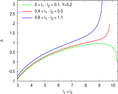
In Fig. 14 (left) $\Delta$ is plotted as a function of $\ell_{1}+\ell_{2}$ for three different values of $\ell_{1}-\ell_{2}$ $(0.1,\,0.5,\,1.0)$; the condition (181) translates into

$$5.0\leq\ell_{1}+\ell_{2}\leq 9.0;$$ (185)

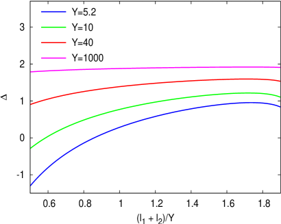
on Fig. 14 (right) the asymptotic limit $\Delta\rightarrow 2$ for very large $Y$ clearly appears (we have taken $\ell_{1}-\ell_{2}=0.1$); it is actually its DLA value [2]; this is not surprising since, in the high energy limit $\gamma_{0}$ becomes very small and sub-leading corrections (hard corrections and running coupling effects) get suppressed.

Figure 14: $\Delta$ as a function of $\ell_{1}+\ell_{2}$ for $Y=5.2$ (left) and its asymptotic behavior (right, $\ell_{1}-\ell_{2}=0.1$)

E.1.3 $\boldsymbol{\Upsilon_{g}}$ and its derivatives

Fig. 15 exhibits the smooth behavior of $\exp{(\Upsilon_{g})}$ as a function of $(\ell_{1}+\ell_{2})$ in the whole range of applicability of our approximation (we have chosen the same values of $(\ell_{1}-\ell_{2})$ as for Fig. 14), and as a function of $(\ell_{1}-\ell_{2})$ for three values of $(\ell_{1}+\ell_{2})$ ($6.0,7.0,8.0$). So, the iterative procedure is safe and corrections stay under control.

Figure 15: $\exp{(\Upsilon_{g})}$ as a function of $\ell_{1}+\ell_{2}$ (left) and, $\ell_{1}-\ell_{2}$ (right) for $Y=5.2$

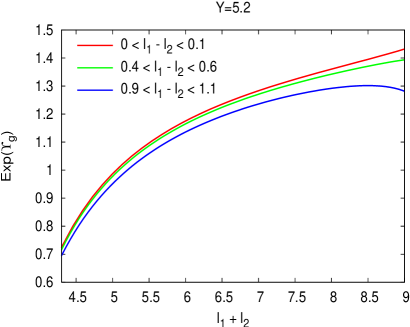
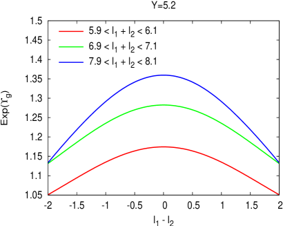
Fig. 16 displays the derivatives of $\Upsilon_{g}$. (186), (187) and (188) have been plotted at $Y=5.2$, for $(\ell_{1}-\ell_{2})=0.1$ (left) and $(\ell_{1}-\ell_{2})=1.0$ (right). The size and shape of these corrections agree with our expectations ($\Upsilon_{g,\ell}=\Upsilon_{g,y}={\cal{O}}(\gamma_{0}^{2})$, $\Upsilon_{g,\ell\,y}={\cal{O}}(\gamma_{0}^{4})$).

For explicit calculations, we have used

$$\Upsilon_{g,\ell}\!\!\! \!\!\!=\!\!\! \!\!\!-\frac{\left[1\!-\!b\left(\psi_{1,\ell}\!+\!\psi_{2,\ell}\!-\!{\beta}\gamma_{0}^{2}\right)\right]\left(\Delta_{\ell}\!-\!a\beta^{2}\gamma_{0}^{4}\right)}{\left(1\!+\!\Delta\!+\!a\beta\gamma_{0}^{2}\right)\left[2\!+\!\Delta\!-\!b\left(\psi_{1,\ell}\!+\!\psi_{2,\ell}\!-\!\,{\beta}\gamma_{0}^{2}\right)\right]}\!-\!\frac{b\left(\psi_{1,\ell\,\ell}\!+\!\psi_{2,\ell\,\ell}\!+\!{\beta^{2}}\gamma_{0}^{4}\right)}{2\!+\!\Delta\!-\!b\left(\psi_{1,\ell}\!+\!\psi_{2,\ell}\!-\!{\beta}\gamma_{0}^{2}\right)},$$ (186)

$$\Upsilon_{g,y}\!\!\! \!\!\!=\!\!\! \!\!\!-\frac{\left[1\!-\!b\left(\psi_{1,\ell}\!+\!\psi_{2,\ell}\!-\!{\beta}\gamma_{0}^{2}\right)\right]\left(\Delta_{y}\!-\!a\beta^{2}\gamma_{0}^{4}\right)}{\left(1\!+\!\Delta\!+\!a\beta\gamma_{0}^{2}\right)\left[2\!+\!\Delta\!-\!b\left(\psi_{1,\ell}\!+\!\psi_{2,\ell}\!-\!{\beta}\gamma_{0}^{2}\right)\right]}\!-\!\frac{b\left(\psi_{1,\ell\,y}\!+\!\psi_{2,\ell\,y}\!+\!{\beta^{2}}\gamma_{0}^{4}\right)}{2\!+\!\Delta\!-\!b\left(\psi_{1,\ell}\!+\!\psi_{2,\ell}\!-\!{\beta}\gamma_{0}^{2}\right)},$$ (187)

$$\Upsilon_{g,\ell\,y}\!\!\! \!\!\!=\!\!\! \!\!\!\frac{\partial\Upsilon_{g,y}}{\partial\ell},$$ (188)

where

$$\Delta_{\ell}\!\! \!\!=\!\! \!\!\gamma_{0}^{-2}\left[\psi_{1,\ell\,\ell}\psi_{2,y}+\psi_{1,\ell}\psi_{2,y\,\ell}+\psi_{2,\ell\,\ell}\psi_{1,y}+\psi_{2,\ell}\psi_{1,y\,\ell}\right]+\beta\gamma_{0}^{2}\Delta,$$ (189)

$$\Delta_{y}\!\! \!\!=\!\! \!\!\gamma_{0}^{-2}\left[\psi_{1,\ell\,y}\psi_{2,y}+\psi_{1,\ell}\psi_{2,y\,y}+\psi_{2,\ell y}\psi_{1,y}+\psi_{2,\ell}\psi_{1,y\,y}\right]+\beta\gamma_{0}^{2}\Delta.$$ (190)

For the expressions of $\psi_{\ell\,\ell}$, $\psi_{\ell\,y}=\psi_{y\,\ell}$ and $\psi_{y\,y}$, the reader is directed to D.3. (188) has been computed numerically (its analytical expression is too heavy to be easily manipulated).

Figure 16: $\Upsilon_{g,\ell}$, $\Upsilon_{g,y}$ and $\Upsilon_{g,\ell\,y}$ as functions of $\ell_{1}+\ell_{2}$ for $Y=5.2$, $\ell_{1}-\ell_{2}=0.1$ (left) and $\ell_{1}-\ell_{2}=1.0$ (right)

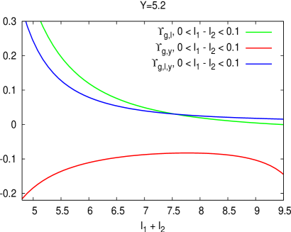
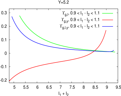
E.1.4 $\boldsymbol{\delta_{1}}$, $\boldsymbol{\delta_{2}}$, $\boldsymbol{\delta_{c}}$

$\delta_{1}$ and $\delta_{2}$ are defined in (71)(76). We also define

$$\delta_{c}=\delta_{1}+\delta_{2}+a\Upsilon_{\ell},$$ (191)

which appears in the numerator of the first line of (70).

Fig. 17 displays the behavior of $\delta_{1}$, $\delta_{2}$ and $\delta_{1}+\delta_{2}$ at $Y=5.2$ for $\ell_{1}-\ell_{2}=0.1$ and $\ell_{1}-\ell_{2}=1.0$. We recall that these curves can only be reasonably trusted in the interval (185).

Though $|\delta_{1}|={\cal{O}}(\gamma_{0})$ (MLLA) should be numerically larger than $|\delta_{2}|={\cal{O}}(\gamma_{0}^{2})$ (NMLLA), it turns out that for relatively large $\gamma_{0}\sim 0.5$ (Y=5.2), $|\delta_{1}|\sim|\delta_{2}|$, and that strong cancellations occur in their sum. As $\gamma_{0}$ decreases (or $Y$ increases) $|\delta_{1}|\gg|\delta_{2}|$, in agreement with the perturbative expansion conditions.

In Fig. 18 we represent $\delta_{c}$ for different values of $Y$; it shows how the sum of corrections (MLLA and NMLLA) stay under control in the confidence interval (185). For $Y=5.2$ one reaches a regime where it becomes slightly larger than $0.1$ away from the region $x_{1}\approx x_{2}$ (see upper curve on the right of Fig. 18) but still, since $1$ (which is the leading term in the numerator of (70)) $\gg 0.1$, our approximation can be trusted.

Figure 17: $\delta_{1}$, $\delta_{2}$ and $\delta_{1}+\delta_{2}$ as functions of $\ell_{1}+\ell_{2}$ for $\ell_{1}-\ell_{2}=0.1$ (left) and $\ell_{1}-\ell_{2}=1.0$ (right)

Figure 18: $\delta_{c}$ as a function of $(\ell_{1}+\ell_{2})/Y$ for $\ell_{1}-\ell_{2}=0.1$ (left) and $\ell_{1}-\ell_{2}=1.0$ (right)

E.1.5 The global role of corrections in the iterative procedure

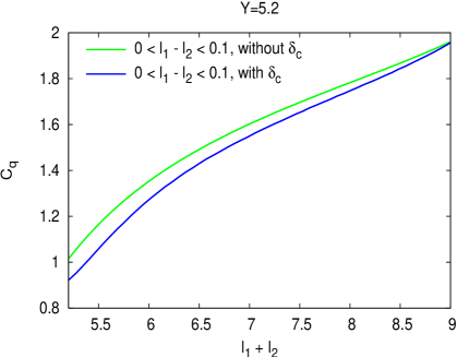
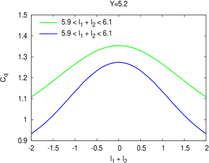
Fig. 19 shows the role of $\delta_{c}$ on the correlation function: we represent the bare function $\exp{\Upsilon_{g}}$ (see 104) as in Fig. 15, together with (70). For $(\ell_{1}-\ell_{2})=0.1$ ($\ell_{1}\approx\ell_{2}$) and $(\ell_{1}-\ell_{2})=1.0$, it is shown how $\delta_{c}$ modifies the shape and size of $\exp{\Upsilon_{g}}$. When $\ell_{1}\neq\ell_{2}$ ($(\ell_{1}-\ell_{2})=1.0$), $\delta_{c}$ decreases the correlations. They are also represented as a function of $(\ell_{1}-\ell_{2})$ when $(\ell_{1}+\ell_{2})$ is fixed ( to $6.0$ and $7.0$). The increase of $\delta_{c}$ as one goes away from the diagonal $\ell_{1}\!\approx\!\ell_{2}$ (see Fig. 18 for $(\ell_{1}-\ell_{2})=1.0$) explain the difference between the green and blue curves; this substantially modifies the tail of the correlations.

When $Y$ gets larger, the role of $\delta_{c}$ decreases: at $Y=7.5$ (LHC conditions) the difference between the two curves becomes negligible.

Figure 19: ${\cal C}_{g}$ (blue) compared with $\exp\Upsilon_{g}$ (green)

E.2 Quark jet

E.2.1 $\boldsymbol{\varphi}$ and its derivatives

Fig. 20 displays the derivatives $\varphi_{\ell}$ and $\varphi_{y}$ together with those $\psi_{\ell}$ and $\psi_{y}$ for the gluon jet, at $Y=5.2$. There sizes and shapes are the same since the logarithmic derivatives of the single inclusive distributions inside a gluon or a quark jet only depend on their shapes (the normalizations cancel in the ratio), which is the same in both cases. The mismatch at small $\ell$ between $\varphi_{\ell}$ and $\psi_{\ell}$ stems from the behavior of $\psi_{\ell\,\ell}$ $\psi_{\ell\,\ell}\stackrel{{\scriptstyle\ell\to 0}}{{\longrightarrow}}-\infty$. Therefore, in the interval of applicability of the soft approximation (128) and (130) can be approximated by $\psi_{\ell}$ and $\psi_{y}$ respectively.

Figure 20: Derivatives $\varphi_{g,\ell}$ and $\varphi_{gy}$ as functions of $\ell$ at fixed $Y=5.2$ (left), compared with $\psi_{\ell}$ and $\psi_{y}$

E.2.2 $\boldsymbol{\tilde{\Delta}(\ell_{1},\ell_{2},Y)}$

The last statement in E.2.1 numerically supports the approximation (131), that is

$$\tilde{\Delta}\approx\Delta+{\cal O}(\gamma_{0}^{2}).$$

We get rid of the heavy ${\cal O}(\gamma_{0}^{2})$ factor in (131) to ease our numerical calculations. Hence, the behavior of $\tilde{\Delta}$ is already given in Fig. 14.

E.2.3 $\boldsymbol{\Upsilon_{q}}$ and its derivatives

The smooth behavior of $\exp\Upsilon_{q}$ is displayed in Fig. 21 as a function of the sum $(\ell_{1}+\ell_{2})$ for fixed $(\ell_{1}-\ell_{2})$ and vice versa. The normalization of $(\exp\Upsilon_{q}-1)$ is roughly twice larger ($\times\frac{Nc}{CF}\approx 2$) than that of $(\exp\Upsilon_{g}-1)$. We then consider derivatives of this expression to get the corresponding iterative corrections shown in Fig. 22. The behavior of $\Upsilon_{q,\ell}({\cal O}(\gamma_{0}^{2}))$, $\Upsilon_{q,y}({\cal O}(\gamma_{0}^{2}))$ and $\Upsilon_{q,\ell\,y}({\cal O}(\gamma_{0}^{4}))$ is in good agreement with our expectations as far as the order of magnitude and the normalization are concerned (see also Fig. 16) .

Figure 21: $\exp{(\Upsilon_{q})}$ as a function of $\ell_{1}+\ell_{2}$ (left) and, $\ell_{1}-\ell_{2}$ (right) for $Y=5.2$

Figure 22: Corrections $\Upsilon_{q,\ell}$, $\Upsilon_{q,y}$ and $\Upsilon_{q,\ell,y}$ as functions of $\ell_{1}+\ell_{2}$ for $\ell_{1}-\ell_{2}=0.1$ (left) and $\ell_{1}-\ell_{2}=1.0$ (right) at $Y=5.2$

E.2.4 $\boldsymbol{\tilde{\delta}_{1}}$, $\boldsymbol{\tilde{\delta}_{2}}$ and $\boldsymbol{\tilde{\delta}_{c}}$

We define

$$\tilde{\delta}_{c}=\tilde{\delta}_{1}+\tilde{\delta}_{2}$$

as it appears in both the numerator and denominator of (91). In Fig. 23 are displayed $\tilde{\delta}_{1}$, $\tilde{\delta}_{2}$ and their sum $\tilde{\delta}_{c}$ as functions of the sum $(\ell_{1}+\ell_{2})$ at fixed $(\ell_{1}-\ell_{2})$ ($\ell_{1}-\ell_{2}=0.1$, left) ($\ell_{1}-\ell_{2}=1.0$, right).

At $Y=5.2$, which corresponds to $\gamma_{0}\approx 0.5$, the relative magnitude of $\tilde{\delta}_{1}$ and $\tilde{\delta}_{2}$ is inverted with respect to what is expected from respectively MLLA and NMLLA corrections (see subsection 4.2). This is the only hint that, at this energy, the expansion should be pushed to include all NMLLA corrections to be reliable.

Large cancellations are, like for gluons, seen to occur in $\tilde{\delta}_{c}$, making the sum of corrections quite small. In order to study the behavior of $\tilde{\delta}_{c}$ as $Y$ increases, it is enough to look at Fig. 24 where we compare $\tilde{\delta}_{c}$ at $Y=5.2,\,6.0,\,7.5$.

Figure 23: $\tilde{\delta}_{1}$, $\tilde{\delta}_{2}$ and $\tilde{\delta}_{1}+\tilde{\delta}_{2}$ as functions of $\ell_{1}+\ell_{2}$ for $\ell_{1}-\ell_{2}=0.1$ (left) and $\ell_{1}-\ell_{2}=1.0$ (right) at $Y=5.2$

Figure 24: $\tilde{\delta}_{c}$ as a function of $(\ell_{1}+\ell_{2})/Y$ for $\ell_{1}-\ell_{2}=0.1$ (left) and $\ell_{1}-\ell_{2}=1.0$ (right) at $Y=5.2,\,6.0,\,7.5$

E.2.5 Global role of corrections in the iterative procedure

It is displayed in Fig. 25. ${\tilde{\delta}_{c}}$ does not affect $\exp\Upsilon_{q}$ near the main diagonal ($\ell_{1}=\ell_{2}$), but it does far from it. We find the same behavior as in the case of a gluon jet.

Figure 25: ${\cal C}_{q}$ (blue) compared with $\exp\Upsilon_{q}$ (green)

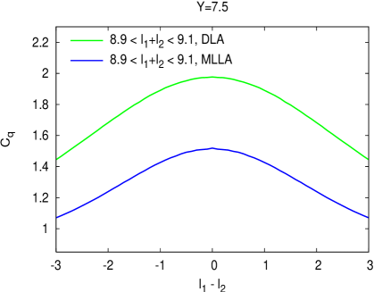
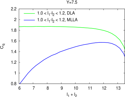
Appendix F COMPARING DLA AND MLLA CORRELATIONS

In Fig. 26 we compare the quark correlator at DLA and MLLA. The large gap between the two curves accounts for the energy balance that is partially restored in MLLA by introducing hard corrections in the partonic evolution equations (terms $\propto$ $a$, $b$ and $\frac{3}{4}$); the DLA curve is obtained by setting $a$, $b$ and $\frac{3}{4}$ to zero in (70) and (91); ${\cal C}_{q}$ is a practically constant function of $\ell_{1}+\ell_{2}$ in almost the whole range, and decreases when $\ell_{1}+\ell_{2}\rightarrow 2Y$ by the running of $\alpha_{s}$. The MLLA increase of ${\cal C}_{q}$ with $\ell_{1}+\ell_{2}$ follows from energy conservation. Similar results are obtained for ${\cal C}_{g}$.

Figure 26: Comparing DLA and MLLA correlations

List of Figures

1. 1 Two-particle correlations and Angular Ordering
2. 2 ${\cal C}_{g}$ for the LEP-I ($Y=7.5$) inside a gluon jet as function of $\ell_{1}+\ell_{2}$ (left) and of $\ell_{1}-\ell_{2}$ (right)
3. 3 ${\cal C}_{q}$ for the LEP-I ($Y=7.5$) inside a quark jet as function of $\ell_{1}+\ell_{2}$ (left) and of $\ell_{1}-\ell_{2}$ (right)
4. 4 Decrease of the correlation for $\ell_{1}\neq\ell_{2}$ at $Y=5.2$, $Y=6.0$ and $Y=7.5$
5. 5 Correlations $R$ between two particles produced in $e^{+}e^{-}\rightarrow q\bar{q}$ compared with the OPAL data and the Fong-Webber approximation
6. 6 Exact ${\cal C}_{g}$ compared with Fong-Webber’s at $Y=5.2$ (left) and $Y=100$ (right)
7. 7 ${\cal C}_{g}$ for the Tevatron ($Y=6.0$) as function of $\ell_{1}+\ell_{2}$ (left) and of $\ell_{1}-\ell_{2}$ (right)
8. 8 ${\cal C}_{q}$ for the Tevatron ($Y=6.0$) as function of $\ell_{1}+\ell_{2}$ (left) and of $\ell_{1}-\ell_{2}$ (right)
9. 9 ${\cal C}_{g}$ for the LHC ($Y=7.5$) inside a gluon jet as function of $\ell_{1}+\ell_{2}$ (left) and of $\ell_{1}-\ell_{2}$ (right)
10. 10 ${\cal C}_{q}$ for the LHC ($Y=7.5$) inside a gluon jet as function of $\ell_{1}+\ell_{2}$ (left) and of $\ell_{1}-\ell_{2}$ (right)
11. 11 Asymptotic behavior of ${\cal C}_{g}$ and ${\cal C}_{q}$ when $Y$ increases
12. 12 Derivatives $\psi_{\ell}$ and $\psi_{y}$ as functions of $\ell$ at fixed $Y=5.2$ (left) and $Y=15$ (right)
13. 13 Double derivatives $\psi_{\ell\,\ell}$, $\psi_{\ell\,y}$ and $\psi_{y\,y}$ as functions of $\ell$ at fixed $Y$
14. 14 $\Delta$ as a function of $\ell_{1}+\ell_{2}$ for $Y=5.2$ (left) and its asymptotic behavior (right, $\ell_{1}-\ell_{2}=0.1$)
15. 15 $\exp{(\Upsilon_{g})}$ as a function of $\ell_{1}+\ell_{2}$ (left) and, $\ell_{1}-\ell_{2}$ (right) for $Y=5.2$
16. 16 $\Upsilon_{g,\ell}$, $\Upsilon_{g,y}$ and $\Upsilon_{g,\ell\,y}$ as functions of $\ell_{1}+\ell_{2}$ for $Y=5.2$, $\ell_{1}-\ell_{2}=0.1$ (left) and $\ell_{1}-\ell_{2}=1.0$ (right)
17. 17 $\delta_{1}$, $\delta_{2}$ and $\delta_{1}+\delta_{2}$ as functions of $\ell_{1}+\ell_{2}$ for $\ell_{1}-\ell_{2}=0.1$ (left) and $\ell_{1}-\ell_{2}=1.0$ (right)
18. 18 $\delta_{c}$ as a function of $(\ell_{1}+\ell_{2})/Y$ for $\ell_{1}-\ell_{2}=0.1$ (left) and $\ell_{1}-\ell_{2}=1.0$ (right)
19. 19 ${\cal C}_{g}$ (blue) compared with $\exp\Upsilon_{g}$ (green)
20. 20 Derivatives $\varphi_{g,\ell}$ and $\varphi_{gy}$ as functions of $\ell$ at fixed $Y=5.2$ (left), compared with $\psi_{\ell}$ and $\psi_{y}$
21. 21 $\exp{(\Upsilon_{q})}$ as a function of $\ell_{1}+\ell_{2}$ (left) and, $\ell_{1}-\ell_{2}$ (right) for $Y=5.2$
22. 22 Corrections $\Upsilon_{q,\ell}$, $\Upsilon_{q,y}$ and $\Upsilon_{q,\ell,y}$ as functions of $\ell_{1}+\ell_{2}$ for $\ell_{1}-\ell_{2}=0.1$ (left) and $\ell_{1}-\ell_{2}=1.0$ (right) at $Y=5.2$
23. 23 $\tilde{\delta}_{1}$, $\tilde{\delta}_{2}$ and $\tilde{\delta}_{1}+\tilde{\delta}_{2}$ as functions of $\ell_{1}+\ell_{2}$ for $\ell_{1}-\ell_{2}=0.1$ (left) and $\ell_{1}-\ell_{2}=1.0$ (right) at $Y=5.2$
24. 24 $\tilde{\delta}_{c}$ as a function of $(\ell_{1}+\ell_{2})/Y$ for $\ell_{1}-\ell_{2}=0.1$ (left) and $\ell_{1}-\ell_{2}=1.0$ (right) at $Y=5.2,\,6.0,\,7.5$
25. 25 ${\cal C}_{q}$ (blue) compared with $\exp\Upsilon_{q}$ (green)
26. 26 Comparing DLA and MLLA correlations

References

- [1] V.N. Gribov and L.N. Lipatov: Sov. J. Nucl. Phys. 15 (1972) 438 and 675; L.N. Lipatov: Sov. J. Nucl. Phys. 20 (1975) 94; A.P. Bukhvostov, L.N. Lipatov and N.P. Popov: Sov. J. Nucl. Phys. 20 (1975) 286; G. Altarelli and G. Parisi: Nucl. Phys. B 126 (1977) 298; Yu.L. Dokshitzer: Sov. Phys. JETP 46 (1977) 641.
- [2] Yu.L. Dokshitzer, V.A. Khoze, A.H. Mueller and S.I. Troyan: Basics of Perturbative QCD, Editions Frontières, Paris, 1991.
- [3] Yu.L. Dokshitzer, V.A. Khoze, S.I. Troyan and A.H. Mueller: Rev. Mod. Phys. 60 (1988) 373-388.
- [4] V.A. Khoze and W. Ochs: Int. J. Mod. Phys. A12 (1997) 2949.
- [5] Yu.L. Dokshitzer, V.S. Fadin and V.A. Khoze: Z. Phys C18 (1983) 37.
- [6] C.P. Fong and B.R. Webber: Phys. Lett. B 241 (1990) 255.
- [7] OPAL Collab.: Phys. Lett. B 287 (1992) 401.
- [8] K. Konishi, A. Ukawa, and G. Veneziano: Nucl. Phys. B 157 (1979) 45.
- [9] OPAL Collab., M.Z. Akrawy et al.: Phys. Lett. B 247 (1990) 617; TASSO Collab., W. Braunschweig et al.: Z. Phys. C 47 (1990) 198; L3 Collab., B. Adeva et al.: L3 Preprint 025 (1991).
- [10] R. Perez-Ramos: “Two particle correlations inside one jet at “Modified Leading logarithmic Approximation” of Quantum Chromodynamics; II: steepest descent evaluation”, in preparation.
- [11] R. Perez-Ramos: Thèse de Doctorat, Université Denis Diderot - Paris 7 (2006).
- [12] R. Perez-Ramos & B. Machet: “MLLA inclusive hadronic distributions inside one jet at high energy colliders”, hep-ph/0512236, JHEP 04 (2006) 043.
- [13] C.P. Fong and B.R. Webber: Phys. Lett. B 229 (1989) 289.
- [14] E.D. Malaza and B.R. Webber: Nucl. Phys. B 267 (1986) 702.
- [15] Yu.L. Dokshitzer, V.S. Fadin and V.A. Khoze: Phys. Lett. B 115 (1982) 242.
- [16] I.S. Gradshteyn and I.M. Ryzhik: Table of Integrals, Series, and Products, Academic Press (New York and London) 1965.
- [17] L.J. Slater, D. Lit., Ph.D. Thesis: Confluent Hypergeometric Functions, Cambridge at the University Press, 1960.