BCS/BEC crossover in Quark Matter
and Evolution of its Static and Dynamic properties
– from the atomic unitary gas to color superconductivity –

Abstract

We study the evolution of dynamic properties of the BCS/BEC (Bose-Einstein Condensate) crossover in a relativistic superfluid as well as its thermodynamics. We put particular focus on the change in the soft mode dynamics throughout the crossover, and find that three different effective theories describe it; these are, the time-dependent Ginzburg-Landau (TDGL) theory in the BCS regime, the Gross-Pitaevskii (GP) theory in the BEC regime, and the relativistic Gross-Pitaevskii (RGP) equation in the relativistic BEC (RBEC) regime. Based on these effective theories, we discuss how the physical nature of soft mode changes in the crossover. We also discuss some fluid-dynamic aspects of the crossover using these effective theories with particular focus on the shear viscosity. In addition to the study of soft modes, we show that the “quantum fluctuation” is present in the relativistic fermion system, which is in contrast to the usual Nozières–Schmit-Rink (NSR) theory. We clarify the physical meaning of the quantum fluctuation, and find that it drastically increases the critical temperature in the weak coupling BCS regime.

I Introduction

Quantum ChromoDynamics (QCD) is expected to exhibit a surprisingly rich phase structure at finite temperature and/or density. The lattice calculations strongly support the conjecture that the nuclear matter undergoes a phase transition to the color-deconfined quark-gluon plasma (QGP) phase at some critical temperature Karsch:1994hm ; Karsch:2003jg . The QGP is a longstanding theoretical issue since the discovery of the asymptotic freedom of QCD Gross:1973ju and is now being searched experimentally in the Relativistic Heavy Ion Collider (RHIC) Arsene:2004fa .

The QGP was originally thought as the weakly coupled plasma and its early conjectured signature Matsui:1986dk was based on this observation, i.e., the strong suppression of heavy $q\bar{q}$ bound states above $T_{c}$. However, the lattice calculations of mesonic spectral functions using the Maximum Entropy Method (MEM) show that the mesonic bound states persist well above the critical temperature Umebo . Moreover, the RHIC data of the collective flow together with the theoretical analyses using the parton cascade simulation Molnar:2001ux and the hydrodynamics Teaney:2003kp suggests the strongly correlated plasma where the partonic cross section is almost $50$ times larger than its perturbative estimate. The recent lattice calculation of the shear viscosity to entropy ratio Nakamura:2004sy in the purely gluonic plasma also shows the value which is a factor 2-3 smaller than its perturbative estimate Arnold:2000dr ; the lattice value is rather close to the minimum bound $(1/4\pi)$ speculated in Kovtun:2004de using the string theory together with the AdS/CFT correspondence Policastro:2001yc .

These theoretical and experimental results show that the characteristics of the QGP are, (i) the existence of the quasi-bound states above $T_{c}$ and (ii) an almost perfect fluidity with small sound-attenuation length Asakawa:2006tc . Some theoretical efforts have been devoted to understanding such a strongly coupled QGP Shuryak:2003ty ; Simonov:2005jj ; Castorina:2005tm ; He:2005bd in which there exist two temperatures, one for the deconfining transition or chiral-restoration ($T_{c}$) and the other for the vanishing of resonances ($T^{*}>T_{c}$). The existence of the mesonic correlation above the chiral-restoration temperature $T_{c}$ was suggested earlier Hatsuda:1985eb using the NJL model analysis Hatsuda:1994pi ; Klevansky:1992qe .

The baryonic matter is also expected to be deconfined to quark matter when it is compressed, which was conjectured in Collins:1974ky or even earlier Itoh:1970uw . Moreover, a variety of color superconducting phases at high baryon density is suggested Bailin:1983bm ; Iwasaki:1994ij ; reviews . It is now widely accepted that the ground state of quark matter is the Color-Flavor-Locked (CFL) phase Alford:1998mk at extremely high density where the gap and critical temperature can be studied by the perturbative Dyson-Schwinger type equations Son:1998uk ; Schafer:1999jg ; Brown:1999aq ; Schafer:1999fe . In contrast, which phase is realized at relatively low density relevant to compact stars still remains a matter of debate because there is no general scheme. However, recent extensive studies based on effective models have revealed that there may arise a surprisingly rich variety of non-BCS exotic phases Alford:2003fq ; Fukushima:2004zq ; Abuki:2004zk ; Ruster:2005jc ; Ciminale:2006sm ; Kitazawa:2006zp ; Fukushima:2006su ; He:2006tn once the kinematical constraints such as the neutrality with respect to the color and electric charges are incorporated. Due to a relatively large strange quark mass, these kinematic effects plays an important role there. Such a stressed pairing is attracting broad interest not only from the QCD community but also from the audience of the atomic polarized Fermi gas Carlson:2005kg ; Son:2005qx ; Gubankova:2006gj ; Mannarelli:2006hr .

Another (and perhaps more direct) source of difficulty in investigating the pairing at low density is the presence of dynamical effects due to its strong coupling nature. As the system goes towards lower density, the gauge coupling grows and some strong coupling effects beyond the mean field approximation (MFA) come to play an important role as pointed out earlier by evaluating the Cooper pair correlation length within the MFA Matsuzaki:1999ww ; Abuki:2001be . Some theoretical efforts to examine the strong coupling effects beyond the MFA were then made with a particular focus on the precursory soft mode Kitazawa:2001ft ; Kitazawa:2003cs ; Kitazawa:2005vr , where non-vanishing diquark correlation and the pseudogap above the critical temperature are reported. Along with this line, the limit temperature $T^{*}$ where the resonances decouple from the spectrum is evaluated both for the chiral and diquark channels in He:2005bd .

Such existence of two temperature scales at strong coupling may be naturally understood in the scenario of the crossover from the BCS pairing to the Bose-Einstein condensate (BEC), i.e., the BCS/BEC crossover eagles ; leggett ; nozieres . The BCS/BEC crossover has been the longstanding theoretical idea first discussed in the context of a theory of superconductivity in low concentration systems such as SrTiO₃ doped with Zr eagles . It has also been introduced to understand the isotropic nature of elementally excitation in ³He superfluid where the spin fluctuation results in strong attraction in ${}^{3}P$ channel leading to the non-$s$-wave pairing leggett . Their work was extended to finite temperature in nozieres where the fluctuation about the MFA was inevitably included within the gaussian approximation. The basic concept of the BCS/BEC crossover is the following; in the weak coupling, the system exhibits the BCS superconductivity due to the attraction and the large density of state at the Fermi surface, while in the strong coupling, the composite bosons are formed at $T^{*}$ prior to their condensation to the bosonic zero mode at $T_{c}<T^{*}$. Although the symmetry breaking pattern is the same in both sides and therefore there is no sharp phase boundary in between, the mechanism of the condensation is completely different in the sense that the former has a dynamical origin while the latter has a rather kinematical origin; in the BEC side, the short range quantum effects are taken only into the structure of composite boson.

So far, the BCS/BEC crossover has been widely discussed in various contexts including not only the liquid ³He leggett or the high $T_{c}$ superconductivity highTc , but also the nuclear matter Lombardo:2001ek , and the magnetically trapped alkali atom systems ohashi02 . Although the crossover scenario in color superconductivity was conjectured in the literature Matsuzaki:1999ww ; Abuki:2001be ; Fukushima:2004bj , the first explicit investigation of this problem was given very recently in Nishida:2005ds where it is shown that the relativistic fermion system exhibits the two-step crossovers; one is the ordinary BCS/BEC crossover but with some unconventional behaviour of the critical temperature brought about by relativistic effects, and the other is the crossover from the BEC to the relativistic BEC (RBEC) kapusta where the critical temperature increases up to the order of Fermi energy. Recently the existence of the RBEC phase has been confirmed at $T=0$ in the Leggett’s flamework and the evolution of collective modes are reported He:2007kd . Investigation of such a relativistic crossover is also performed in a boson-fermion model Nawa:2005sb ; Deng:2006ed which together with a chemical equilibrium condition enables us to describe the crossover thermodynamics with a boson mass or chemical potential controlled by hand. A possible importance of the diquark BEC in QCD phase diagram at low density is demonstrated in a model calculation Rezaeian:2006yj . The BCS/BEC crossover is also discussed in Babaev:1999iz with possible relevance to the chiral transition using the nonlinear sigma model. Moreover, in recent work Castorina:2005tm , it is discussed with special emphasis on the chiral pseudogap phase above $T_{c}$.

As above, the BCS/BEC crossover is discussed in the QCD context to give an insight into the strong coupling nature of the quark-gluon plasma in either low or high density. However, how the transport and hydrodynamic properties change throughout the crossover remains unclarified; this is interesting because it may provide some unified view on the two apparently independent aspects of QGP, i.e., (i) the survival of the bound states above $T_{c}$ and (ii) the perfect liquidity.

It is also worth mentioning that the hydrodynamic properties of the unitary Fermi gas have recently attracted considerable attention both experimentally Thomas ; Grimm-collective ; Thomas-breakdown ; Thomas-2transitions ; OHara ; Salomon-intE and theoretically Gelman:2004fj ; Schaefer:2007pr ; Son:2005tj . The unitary Fermi gas is the intermediate of the BCS/BEC crossover, where the $s$-wave scattering length diverges. Such strongly coupled system can be created in the atomic traps with the external magnetic field fine tuned to the Feshbach resonance regal04 . It provides us with a theoretical challenge to describe such a unique many body system which is universal in the sense that there is no intrinsic dimensionful parameter except for temperature and density Nishida:2006br . Understanding such system also may shed light on the physics of high $T_{c}$ superconductivity highTc , and possibly, the QGP.

The aim of this paper is to understand how the transport properties of the relativistic fermion system, as well as its thermodynamics, change throughout the BCS/BEC crossover. In order to do this, we first formulate the relativistic Nozières–Schmitt-Rink (NSR) framework extending our earlier work Nishida:2005ds to fermions having SU$(2)_{\rm F}$ flavor and SU$(3)_{\rm c}$ color with a little refined regularization scheme. We then derive the effective theory for soft modes and study how this effective theory changes as the system moves from BCS to (R)BEC regime. Based on this effective theory, we will discuss some of fluid dynamic aspects of the crossover with particular focus on the shear viscosity and its ratio to the entropy which serves as a measure of “perfect liquidity”.

The rest of this paper is organized as follows: In Sec. II, we formulate the Nozières–Schmit-Rink theory for a relativistic fermion system. It turns out that, in contrast to the nonrelativistic system, the relativistic fermion system has an additional source of fluctuation, i.e., the “quantum fluctuation” which we have just ignored in our previous study Nishida:2005ds . Our framework is not restricted to quark matter, and may be used for the other relativistic fermion systems such as a possible neutrino superfluid trapped in compact stars at the early stage of their thermal evolution Kapusta:2004gi . In Sec. III, we discuss the static part of problem, i.e., thermodynamics, the pair size, the spectrum, etc. In Sec. IV, we derive the effective theory for soft modes and study how it evolves with the crossover. In addition, we discuss the shear viscosity to entropy ratio based on the effective theory. In Sec. V, we investigate the density dependence of the crossover. We also study how the “quantum fluctuation” affects the crossover. In Sec. VI, we make concluding remarks and perspectives.

II Formulation

In this section, we extend the Nozières–Schmit-Rink theory so as to apply it to study relativistic fermions interacting via a point attraction. In Sec. II.1, we derive the thermodynamic potential up to the gaussian fluctuation about the MFA. In Sec. II.2, we introduce an intuitive representation of the thermodynamic potential in terms of the spectral density. In Sec. II.3, we introduce the in-medium phase shift which enables us to handle easily the fluctuation effect to the number conservation. In Sec. II.4, we discuss the Thouless criterion and present how to renormalize it using the low energy scattering parameter, the scattering length. In Sec. II.5, we give the renormalization scheme for the dynamic pair susceptibility. In Sec. II.6, we end up with a couple of basic equations, i.e., the number conservation, and the Thouless criterion.

II.1 Nozières–Schmit-Rink theory for a relativistic fermion system

We start with the following four-Fermi model inspired by the one-gluon exchange (OGE) Nishida:2005ds ,

$${\mathcal{L}}=\bar{q}(i\hbox to5.30904pt{\hbox to0.0pt{\hbox to5.30904pt{\hss/\hss}\hss}\hbox{$\partial$}}+\hbox to6.02548pt{\hbox to0.0pt{\hbox to6.02548pt{\hss/\hss}\hss}\hbox{$\mu$}}-m)q-\frac{g^{2}}{2}\sum_{a=1}^{8}\bar{q}T^{a}\gamma_{\mu}q\,\bar{q}T^{a}\gamma^{\mu}q.$$ (1)

Here quark has $N_{c}=3$ colors and $N_{f}=2$ flavors, and $T^{a}=\lambda^{a}/2$ is the Gell-Mann matrix for color. At high density, we expect the pair formation in the $J^{P}=0^{+}$, and the color-flavor triplet channel Bailin:1983bm , i.e.,

$$(P_{\eta})_{ab}^{ij}=iC\gamma_{5}\epsilon^{ij}\epsilon_{abc}.$$ (2)

The indices $\{i,j,\cdots\}$ represent flavors and $\{a,b,\cdots\}$ indicate colors. Fierz transformation allows us to re-write the Lagrangian Eq. (1) as follows.

$$\begin{array}[]{rcl}{\mathcal{L}}&=&\bar{q}(i\hbox to5.30904pt{\hbox to0.0pt{\hbox to5.30904pt{\hss/\hss}\hss}\hbox{$\partial$}}+\hbox to6.02548pt{\hbox to0.0pt{\hbox to6.02548pt{\hss/\hss}\hss}\hbox{$\mu$}}-m)q+\frac{G}{4}\sum_{\eta=1}^{3}[iq^{t}P_{\eta}q][i\bar{q}\bar{P}_{\eta}\bar{q}^{t}]\\[8.61108pt] &&+\frac{G}{4}\sum_{\eta=1}^{3}[iq^{t}P_{\eta}\gamma_{5}q][i\bar{q}\bar{P}_{\eta}\gamma_{5}\bar{q}^{t}]\cdots\\[8.61108pt] \end{array},$$ (3)

with $G=\frac{N_{c}+1}{4N_{c}}g^{2}$. Though we find the attraction in the scaler $q\bar{q}$ channel, we shall ignore this channel throughout this paper; consequently, our framework is not reliable in the vicinity of the chiral-restoration density. By introducing a spinor doublet $Q=(q,\bar{q})^{t}$, we write

$$\begin{array}[]{rcl}{\mathcal{L}}&=&\displaystyle\frac{1}{2}\bar{Q}\left(\begin{array}[]{cc}i\hbox to5.30904pt{\hbox to0.0pt{\hbox to5.30904pt{\hss/\hss}\hss}\hbox{$\partial$}}+\hbox to6.02548pt{\hbox to0.0pt{\hbox to6.02548pt{\hss/\hss}\hss}\hbox{$\mu$}}-m&0\\ 0&i\hbox to5.30904pt{\hbox to0.0pt{\hbox to5.30904pt{\hss/\hss}\hss}\hbox{$\partial$}}^{t}-\hbox to6.02548pt{\hbox to0.0pt{\hbox to6.02548pt{\hss/\hss}\hss}\hbox{$\mu$}}^{t}+m\\ \end{array}\right)Q\\[8.61108pt] &&\displaystyle+\frac{G}{4}\bar{Q}\left(\begin{array}[]{cc}0&0\\ P_{\eta}&0\\ \end{array}\right)Q\bar{Q}\left(\begin{array}[]{cc}0&\bar{P}_{\eta}\\ 0&0\\ \end{array}\right)Q.\end{array}$$ (4)

Here, we have defined $\bar{P}_{\eta}=\gamma_{0}(P_{\eta})^{\dagger}\gamma_{0}$. Then the partition function is

$$Z=\int{\mathcal{D}}Q\exp\biggl{[}-\int_{0}^{\beta}d\tau\int d\mbox{\boldmath$x$}{\mathcal{L}}_{E}(Q)\biggr{]},$$ (5)

where ${\mathcal{L}}_{E}=-{\mathcal{L}}|_{t\to-i\tau}$ is the Lagrangian density in the Euclid space, which is periodic in the imaginary time interval $[0,\beta]$. Introducing the Hubberd-Stratnobich fields

$$\begin{array}[]{rcl}\Delta_{\eta}(\tau,x)&=&\frac{G}{2}\biggl{\langle}\bar{Q}\left(\begin{array}[]{cc}0&0\\ P_{\eta}&0\\ \end{array}\right)Q\biggr{\rangle},\\[4.30554pt] \Delta^{*}_{\eta}(\tau,x)&=&\frac{G}{2}\biggl{\langle}\bar{Q}\left(\begin{array}[]{cc}0&\bar{P}_{\eta}\\ 0&0\\ \end{array}\right)Q\biggr{\rangle},\\[4.30554pt] \end{array}$$ (6)

and integrating out quark fields, we obtain

$$\begin{array}[]{rcl}Z&=&\displaystyle\int{\mathcal{D}}\Delta{\mathcal{D}}\Delta^{*}\exp\left[-\int d\tau d\mbox{\boldmath$x$}\left(\frac{|\Delta(-i\tau,\mbox{\boldmath$x$})|^{2}}{G}\right)\right]\\[8.61108pt] &&\displaystyle\times\exp\left[\frac{1}{2}{\rm log}\,\underset{(x,y)}{\rm Det}\left(\begin{array}[]{cc}S_{Fx,y}^{-1}&\bar{P}_{\eta}\Delta(x)\delta_{x,y}\\ P_{\eta}\Delta^{*}(x)\delta_{x,y}&\bar{S}_{Fx,y}^{-1}\end{array}\right)\right].\\[8.61108pt] \end{array}$$ (7)

Here the bare propagator is defined by

$$\begin{array}[]{rcl}S_{Fx,y}^{-1}&=&(i\hbox to5.30904pt{\hbox to0.0pt{\hbox to5.30904pt{\hss/\hss}\hss}\hbox{$\partial$}}+\hbox to6.02548pt{\hbox to0.0pt{\hbox to6.02548pt{\hss/\hss}\hss}\hbox{$\mu$}}-m)\delta_{x,y},\\[8.61108pt] \bar{S}_{Fx,y}^{-1}&=&\gamma_{5}CS_{Fy,x}^{-1}C\gamma_{5}.\end{array}$$ (8)

$\delta_{x,y}$ is the delta function antiperiodic in the imaginary time $\tau$; in momentum space,

$$\delta_{x,y}=T\sum_{n}\int\frac{d\mbox{\boldmath$p$}}{(2\pi)^{3}}e^{-i\omega_{n}(\tau_{x}-\tau_{y})+i\mbox{\boldmath$\scriptstyle p$}\cdot(\mathstrut\mbox{\scriptsize{\boldmath$x$}}\mathstrut-\mathstrut\mbox{\scriptsize{\boldmath$y$}}\mathstrut)},$$ (9)

with $\omega_{n}$ being the fermionic Matsubara-frequency. Introducing the following notations for the Nambu-Gor’kov propagator and self energy,

$$\begin{array}[]{rcl}\mbox{\boldmath$S$}_{Fx,y}^{-1}&=&\left(\begin{array}[]{cc}S_{Fx,y}^{-1}&0\\ 0&\bar{S}_{Fx,y}^{-1}\end{array}\right),\\[12.91663pt] -\mbox{\boldmath$\Sigma$}_{x,y}&=&\left(\begin{array}[]{cc}0&\bar{P}_{\eta}\Delta_{\eta}(x)\delta_{x,y}\\ P_{\eta}\Delta^{*}_{\eta}(x)\delta_{x,y}&0\end{array}\right),\\[8.61108pt] \end{array}$$ (10)

we can write the partition function in the following form where the fluctuation contribution is factorized:

$$Z(\mu,T)\equiv e^{-\beta\Omega(\mu,T)}=Z_{0}(\mu,T)Z_{\rm fluc}(\mu,T),$$ (11)

where $Z_{\rm fluc}$ is the part coming from the fluctuation:

$$\begin{array}[]{rcl}Z_{\rm fluc}&=&\displaystyle\int{\mathcal{D}}\Delta{\mathcal{D}}\Delta^{*}\exp\left[-\int d\tau d\mbox{\boldmath$x$}\left(\frac{|\Delta_{\eta}(-i\tau,\mbox{\boldmath$x$})|^{2}}{G}\right)\right]\\[8.61108pt] &&\displaystyle\times\exp\left[\frac{1}{2}{\rm log}\,\underset{(x,y)}{\rm Det}\left(\delta_{x,y}-\sum_{z}\mbox{\boldmath$S$}_{Fx,z}\mbox{\boldmath$\Sigma$}_{z,y}\right)\right].\\[8.61108pt] \end{array}$$ (12)

$\sum_{z}$ is a shorthand notation of $\int_{0}^{\beta}d\tau_{z}\int d\mbox{\boldmath$z$}$. The free partition function $Z_{0}$ is $e^{-\beta\Omega_{0}}$ with $\Omega_{0}$ being the thermodynamic potential for free (massive) quarks:

$$\begin{array}[]{rcl}\displaystyle\frac{\Omega_{0}}{V}&=&\displaystyle-2N_{f}N_{c}\,T\sum_{\alpha=\pm}\int\!\!\!\frac{d\mbox{\boldmath$p$}}{(2\pi)^{3}}\log\left(1+e^{-\epsilon_{p\alpha}/T}\right),\\[4.30554pt] \end{array}$$ (13)

where $\epsilon_{p\pm}=\sqrt{\mathstrut m^{2}+p^{2}}\mp\mu$, and the vacuum fluctuation which has no dependence on $(\mu,T)$ is suppressed.

Up to quadratic order in $(\Delta,\Delta^{*})$ (the gaussian approximation), we have

$$Z_{\rm fluc}\equiv e^{-\beta\Omega_{\rm fluc}}=\prod_{\eta,N,\mathstrut\mbox{\scriptsize{\boldmath$P$}}\mathstrut}\int d\Delta_{\eta}(i\Omega_{N},\mbox{\boldmath$P$})d\Delta^{*}_{\eta}(i\Omega_{N},\mbox{\boldmath$P$})\exp\left[-\frac{T}{V}\left(\frac{1}{G}-\chi_{\mu,T}(i\Omega_{N},\mbox{\boldmath$P$})\right)|\Delta_{\eta}(i\Omega_{N},\mbox{\boldmath$P$})|^{2}\right],$$ (14)

where $\Omega_{N}$ and $P$ denote the bosonic Matsubara-frequency and momentum. The pair correlation function $\chi_{\mu,T}(i\Omega_{N},\mbox{\boldmath$P$})$ at one-loop level is defined by Kitazawa:2001ft ; Kitazawa:2005vr

$$\begin{array}[]{rcl}\displaystyle\chi_{\mu,T}(i\Omega_{N},\mbox{\boldmath$P$})&=&\displaystyle 2T\sum_{n}\int\!\!\!\frac{d\mbox{\boldmath$q$}}{(2\pi)^{3}}\mbox{tr}\Big{[}S_{F}(i\omega_{n}+i\Omega_{N},\mbox{\boldmath$q$}+\mbox{\boldmath$P$})S_{F}(-i\omega_{n},-\mbox{\boldmath$q$})\Big{]}\\[8.61108pt] &=&\displaystyle-2\int\!\!\!\frac{d\mbox{\boldmath$q$}}{(2\pi)^{3}}\bigg{(}1+\frac{m^{2}+\mbox{\boldmath$q$}\cdot(\mbox{\boldmath$q$}+\mbox{\boldmath$P$})}{E_{\mathstrut\mbox{\scriptsize{\boldmath$q$}}\mathstrut}E_{\mathstrut\mbox{\scriptsize{\boldmath$q$}}\mathstrut+\mathstrut\mbox{\scriptsize{\boldmath$P$}}\mathstrut}}\bigg{)}\frac{1-f_{F}(E_{\mathstrut\mbox{\scriptsize{\boldmath$q$}}\mathstrut+\mathstrut\mbox{\scriptsize{\boldmath$P$}}\mathstrut}-\mu)-f_{F}(E_{\mathstrut\mbox{\scriptsize{\boldmath$q$}}\mathstrut}-\mu)}{i\Omega_{N}+2\mu-E_{\mathstrut\mbox{\scriptsize{\boldmath$q$}}\mathstrut+\mathstrut\mbox{\scriptsize{\boldmath$P$}}\mathstrut}-E_{\mathstrut\mbox{\scriptsize{\boldmath$q$}}\mathstrut}}\\[8.61108pt] &&\displaystyle-4\int\!\!\!\frac{d\mbox{\boldmath$q$}}{(2\pi)^{3}}\bigg{(}1-\frac{m^{2}+\mbox{\boldmath$q$}\cdot(\mbox{\boldmath$q$}+\mbox{\boldmath$P$})}{E_{\mathstrut\mbox{\scriptsize{\boldmath$q$}}\mathstrut}E_{\mathstrut\mbox{\scriptsize{\boldmath$q$}}\mathstrut+\mathstrut\mbox{\scriptsize{\boldmath$P$}}\mathstrut}}\bigg{)}\frac{-f_{F}(E_{\mathstrut\mbox{\scriptsize{\boldmath$q$}}\mathstrut+\mathstrut\mbox{\scriptsize{\boldmath$P$}}\mathstrut}-\mu)+f_{F}(E_{\mathstrut\mbox{\scriptsize{\boldmath$q$}}\mathstrut}+\mu)}{i\Omega_{N}+2\mu-E_{\mathstrut\mbox{\scriptsize{\boldmath$q$}}\mathstrut+\mathstrut\mbox{\scriptsize{\boldmath$P$}}\mathstrut}+E_{\mathstrut\mbox{\scriptsize{\boldmath$q$}}\mathstrut}}\\[8.61108pt] &&\displaystyle+2\int\!\!\!\frac{d\mbox{\boldmath$q$}}{(2\pi)^{3}}\bigg{(}1+\frac{m^{2}+\mbox{\boldmath$q$}\cdot(\mbox{\boldmath$q$}+\mbox{\boldmath$P$})}{E_{\mathstrut\mbox{\scriptsize{\boldmath$q$}}\mathstrut}E_{\mathstrut\mbox{\scriptsize{\boldmath$q$}}\mathstrut+\mathstrut\mbox{\scriptsize{\boldmath$P$}}\mathstrut}}\bigg{)}\frac{1-f_{F}(E_{\mathstrut\mbox{\scriptsize{\boldmath$q$}}\mathstrut+\mathstrut\mbox{\scriptsize{\boldmath$P$}}\mathstrut}+\mu)-f_{F}(E_{\mathstrut\mbox{\scriptsize{\boldmath$q$}}\mathstrut}+\mu)}{i\Omega_{N}+2\mu+E_{\mathstrut\mbox{\scriptsize{\boldmath$q$}}\mathstrut+\mathstrut\mbox{\scriptsize{\boldmath$P$}}\mathstrut}+E_{\mathstrut\mbox{\scriptsize{\boldmath$q$}}\mathstrut}},\\[8.61108pt] \end{array}$$ (15)

where $S_{F}(\omega_{n},\mbox{\boldmath$p$})$ is the Fourier transform of the fermion propagator $S_{Fx,y}$, i.e., the inverse of Eq. (8). Integrating out the gaussian fluctuation leads to the following expression for thermodynamic potential.

$$\Omega(\mu,T)=\Omega_{0}(\mu,T)+\Omega_{\rm fluc}(\mu,T),\\$$ (16)

with the gaussian fluctuation being defined by

$$\begin{array}[]{rcl}\Omega_{\rm fluc}&=&\displaystyle d_{B}T\sum_{N:\mbox{\scriptsize even}}\int\!\!\!\frac{d\mbox{\boldmath$P$}}{(2\pi)^{3}}\log\left[\frac{1}{G}-\chi_{\mu,T}(i\Omega_{N},\mbox{\boldmath$P$})\right].\\[12.91663pt] &&\displaystyle-d_{B}\int_{-\infty}^{\infty}d\Omega\int\!\!\!\frac{d\mbox{\boldmath$P$}}{(2\pi)^{3}}\log\left[\frac{1}{G}-\chi_{0}(i\Omega,\mbox{\boldmath$P$})\right],\\[8.61108pt] \end{array}$$ (17)

where $d_{B}=\frac{N_{c}(N_{c}-1)}{2}$ is the number of “flavors” of boson and $\chi_{0}\equiv\chi_{\mu=0,T=0}$; we have subtracted the “vacuum” contribution at $\mu=T=0$, which in general leads a $G$-dependent fermion mass and wavefunction renormalization through a Hartree and higher order terms tokumitsu . Some notes are in order here. (i) The fluctuation is symmetric under $\mu\leftrightarrow-\mu$ as it should be. This is guaranteed by the charge conjugation property $\chi_{-\mu,T}(-i\Omega_{N},\mbox{\boldmath$P$})|=\chi_{\mu,T}(i\Omega_{N},\mbox{\boldmath$P$})$. (ii) The above formula is analytic above some $T_{c}$ below which the system undergoes the transition to pairing phase.

The dynamic pair susceptibility $\Gamma(\omega,\mbox{\boldmath$P$})$ can be obtained by the analytic continuation of pair correlation, Eq. (15), to the real $\omega$-axis:

$$\Gamma_{\mu,T}^{-1}(\omega,\mbox{\boldmath$P$})=\frac{1}{G}-\chi_{\mu,T}(\omega+i\delta,\mbox{\boldmath$P$}).$$ (18)

II.2 Thermodynamic potential in terms of spectral density

We introduce a spectral density at some coupling strength $G=\mathcal{G}$ by

$$-\frac{1}{1/\mathcal{G}-\chi_{\mu,T}(i\Omega_{N},\mbox{\boldmath$P$})}=\int_{-\infty}^{\infty}\frac{d\omega}{\pi}\frac{\rho^{\mathcal{G}}_{\mu,T}(\omega,\mbox{\boldmath$P$})}{i\Omega_{N}-\omega}.$$ (19)

It is clear that the spectral density is related to the imaginary part of the dynamic pair susceptibility at $\mathcal{G}$.

$$\rho^{\mathcal{G}}_{\mu,T}(\omega,\mbox{\boldmath$P$})={{\rm Im}\,}\Gamma_{\mu,T}^{\mathcal{G}}(\omega,\mbox{\boldmath$P$})$$ (20)

To express the thermodynamic potential in terms of the spectral density, we differentiate and integrate Eq. (17) with respect to $G$. We obtain

$$\begin{array}[]{rcl}\Omega_{\rm fluc}&=&\displaystyle d_{B}\int_{0}^{G}\frac{d\mathcal{G}}{\mathcal{G}^{2}}\int_{-\infty}^{\infty}\frac{d\omega}{\pi}\frac{d\mbox{\boldmath$P$}}{(2\pi)^{3}}{T}\sum_{N}\frac{\omega\rho^{\mathcal{G}}_{\mu,T}(\omega,\mbox{\boldmath$P$})}{\Omega_{N}^{2}+\omega^{2}}\\[12.91663pt] &&\displaystyle-(\mbox{$T=\mu=0$ part})\end{array}$$ (21)

Because of the identity $\rho_{-\mu,T}^{\mathcal{G}}(\omega,\mbox{\boldmath$P$})=-\rho_{\mu,T}^{\mathcal{G}}(-\omega,\mbox{\boldmath$P$})$, the thermodynamic potential still possesses the charge conjugation symmetry. By performing the Matsubara-summation, we obtain

$$\begin{array}[]{rcl}\Omega_{\rm fluc}&=&\displaystyle-d_{B}\int_{0}^{G}\!\frac{d\mathcal{G}}{\mathcal{G}^{2}}\int_{-\infty}^{\infty}\!\frac{d\omega}{\pi}\frac{d\mbox{\boldmath$P$}}{(2\pi)^{3}}\tilde{f}_{B}(\omega)\rho^{\mathcal{G}}_{\mu,T}(\omega,\mbox{\boldmath$P$})\\[8.61108pt] &&\displaystyle-d_{B}\int_{0}^{G}\!\frac{d\mathcal{G}}{\mathcal{G}^{2}}\int_{-\infty}^{\infty}\!\frac{d\omega}{\pi}\frac{d\mbox{\boldmath$P$}}{(2\pi)^{3}}\frac{\epsilon(\omega)}{2}{\it\Delta}\rho^{\mathcal{G}}_{\mu,T}(\omega,\mbox{\boldmath$P$}).\end{array}$$ (22)

where $\tilde{f}_{B}(\omega)=f_{B}(\omega)+\theta(-\omega)$ with $f_{B}(\omega)=1/(e^{\beta\omega}-1)$ being the bose distribution function. We have defined the in-medium spectral shift ${\it\Delta}\rho^{\mathcal{G}}_{\mu,T}(\omega,\mbox{\boldmath$P$})=\rho^{\mathcal{G}}_{\mu,T}(\omega,\mbox{\boldmath$P$})-\rho_{0}^{\mathcal{G}}(\omega,\mbox{\boldmath$P$})$ with $\rho_{0}^{\mathcal{G}}(\omega,\mbox{\boldmath$P$})=\rho_{0,0}^{\mathcal{G}}(\omega,\mbox{\boldmath$P$})$ being the spectral density at $\mu=T=0$. We denote the first term by $\Omega_{\rm NSR}$, and the second term by $\Omega_{\rm qfl}$ hereafter. The total fluctuation is then the sum of these two pieces.

$$\Omega_{\rm fluc}=\Omega_{\rm NSR}+\Omega_{\rm qfl},$$ (23)

where

$$\Omega_{\rm NSR}=\displaystyle-d_{B}\int_{0}^{G}\!\frac{d\mathcal{G}}{\mathcal{G}^{2}}\int_{-\infty}^{\infty}\!\frac{d\omega}{\pi}\frac{d\mbox{\boldmath$P$}}{(2\pi)^{3}}\tilde{f}_{B}(\omega)\rho^{\mathcal{G}}_{\mu,T}(\omega,\mbox{\boldmath$P$}),$$ (24)

and

$$\Omega_{\rm qfl}=-d_{B}\int_{0}^{G}\!\frac{d\mathcal{G}}{\mathcal{G}^{2}}\int_{-\infty}^{\infty}\!\frac{d\omega}{\pi}\frac{d\mbox{\boldmath$P$}}{(2\pi)^{3}}\frac{\epsilon(\omega)}{2}{\it\Delta}\rho^{\mathcal{G}}_{\mu,T}(\omega,\mbox{\boldmath$P$}).$$ (25)

$\Omega_{\rm NSR}$ is the Nozières–Schmit-Rink correction to the thermodynamic potential and roughly corresponds to the thermal fluctuation, while $\Omega_{\rm qfl}$ can be regarded as the quantum fluctuation which is ignored in the nonrelativistic Nozières–Schmit-Rink theory. If we take the limit $T\to 0$, the former goes to zero, but the latter remains:

$$\begin{array}[]{l}-d_{B}\int_{0}^{G}\!\frac{d\mathcal{G}}{\mathcal{G}^{2}}\int_{-\infty}^{\infty}\!\frac{d\omega}{\pi}\frac{d\mathstrut\mbox{\scriptsize{\boldmath$P$}}\mathstrut}{(2\pi)^{3}}\frac{\epsilon(\omega)}{2}\left[\rho^{\mathcal{G}}_{\mu,0}(\omega,\mbox{\boldmath$P$})-\rho^{\mathcal{G}}_{0}(\omega,\mbox{\boldmath$P$})\right].\\[8.61108pt] \end{array}$$ (26)

$\Omega_{\rm qfl}$ may play an important role at low temperatures, but we shall ignore this contribution for a while because (i) the fluctuation itself is less significant in the weak coupling (low $T_{c}$) regime, and (ii) the charge conjugation symmetry is maintained even if $\Omega_{\rm qfl}$ is ignored. We will come back to this problem in Sec. V where we examine how large this “quantum correction” is.

II.3 Thermodynamic potential in terms of phase shift

It is sometimes more convenient to express the thermodynamic potential in terms of the in-medium phase shift rather than the spectral density. It may be defined by the integration of the spectral density:

$$\begin{array}[]{rcl}\displaystyle\int_{0}^{G}\!\frac{d\mathcal{G}}{\mathcal{G}^{2}}\rho^{\mathcal{G}}_{\mu,T}(\omega,\mbox{\boldmath$P$})&=&\displaystyle\frac{i}{2}\log\left(\frac{\frac{1}{G}-\chi_{\mu,T}(\omega+i\delta,\mbox{\boldmath$P$})}{\frac{1}{G}-\chi_{\mu,T}(\omega-i\delta,\mbox{\boldmath$P$})}\right)\\[17.22217pt] &\equiv&\delta_{\mu,T}(\omega,\mbox{\boldmath$P$}),\end{array}$$ (27)

i.e., the argument of the dynamic pair susceptibility

$$\frac{\frac{1}{G}-\chi_{\mu,T}(\omega\pm i\delta,\mbox{\boldmath$P$})}{\big{|}\frac{1}{G}-\chi_{\mu,T}(\omega,\mbox{\boldmath$P$})\big{|}}=e^{\mp i\delta_{\mu,T}(\omega,\mathstrut\mbox{\scriptsize{\boldmath$P$}}\mathstrut)}.$$ (28)

The phase shift possesses the charge conjugation $\delta_{-\mu,T}(-\omega,\mbox{\boldmath$P$})=-\delta_{\mu,T}(\omega,\mbox{\boldmath$P$})$. Using this phase shift, we can express $\Omega_{\rm NSR}$ and $\Omega_{\rm qfl}$ as

$$\begin{array}[]{rcl}\Omega_{\rm NSR}&=&\displaystyle\!\!-d_{B}\int_{-\infty}^{\infty}\!\frac{d\omega}{\pi}\frac{d\mbox{\boldmath$P$}}{(2\pi)^{3}}\tilde{f}_{B}(\omega)\delta_{\mu,T}(\omega,\mbox{\boldmath$P$}),\\[12.91663pt] \Omega_{\rm qfl}&=&\displaystyle\!\!-d_{B}\int_{-\infty}^{\infty}\!\frac{d\omega}{\pi}\frac{d\mbox{\boldmath$P$}}{(2\pi)^{3}}\frac{\epsilon(\omega)}{2}{\it\Delta\delta_{\mu,T}}(\omega,\mbox{\boldmath$P$}),\\[4.30554pt] \end{array}$$ (29)

where the in-medium shift of the phase shift is defined by ${\it\Delta}\delta_{\mu,T}(\omega,\mbox{\boldmath$P$})\equiv\delta_{\mu,T}(\omega,\mbox{\boldmath$P$})-\delta_{0}(\omega,\mbox{\boldmath$P$})$ with $\delta_{0}(\omega,\mbox{\boldmath$P$})\equiv\delta_{0,0}(\omega,\mbox{\boldmath$P$})$ being the phase shift in vacuum. $\Omega_{\rm NSR}$ is exactly of the same form as that derived by the Nozières–Schmitt-Rink nozieres .

II.4 Thouless criterion and the renormalization of the coupling

In the weak coupling regime, the Thouless condition determines the critical temperature. This condition ensures the divergence of the long wavelength limit of the dynamic pair susceptibility at the critical temperature for a given chemical potential $\mu$:

$$\Gamma^{-1}_{\mu,T_{c}}(0,\mbox{\boldmath$0$})=\frac{1}{G}-\chi_{\mu,T_{c}}(0,\mbox{\boldmath$0$})=0.$$ (30)

$\chi_{\mu,T}(0,\mbox{\boldmath$0$})$ can be calculated as

$$\chi_{\mu,T_{c}}(0,\mbox{\boldmath$0$})=2\int\!\!\frac{d\mbox{\boldmath$q$}}{(2\pi)^{3}}\frac{\tanh\frac{E_{q}-\mu}{2T_{c}}}{E_{q}-\mu}+(\mu\rightarrow-\mu).$$ (31)

which is quadratically divergent. Accordingly, the critical temperature should depend on the cutoff as

$$T_{c}=\Lambda f(m/\Lambda,\mu/\Lambda,G\Lambda^{2}),$$ (32)

where $f$ is some function. We can reduce the cutoff dependence via the partial renormalization of the coupling using the low energy information about the scattering $T$-matrix. We here consider the fermion-fermion scattering $(f(1)+f(2)\to f(3)+f(4))$ with $(1,2,3,4)$ labeling the momentum, color, flavor and helicity of each quark, as $(\mbox{``1''}=(\mbox{\boldmath$p$},a,i,h_{1}),\,\mbox{``2''}=(-\mbox{\boldmath$p$},b,j,h_{2})),\,(\mbox{``3''}=(\mbox{\boldmath$k$},c,k,h_{3}),\,\mbox{``4''}=(-\mbox{\boldmath$k$},d,l,h_{4}))$. Then the on-shell $T$-matrix can be parameterized as

$$T(12\rightarrow 34)=T(\mbox{\boldmath$p$},\mbox{\boldmath$k$})\big{(}\Gamma_{12}\Gamma_{34}-(3\leftrightarrow 4)\big{)},$$ (33)

where $\Gamma_{12}$ is defined by

$$\Gamma_{12}=\frac{\varepsilon_{ab}}{\sqrt{\mathstrut 2}}\frac{\varepsilon_{ij}}{\sqrt{\mathstrut 2}}\frac{\sigma^{3}_{h_{1}h_{2}}}{\sqrt{\mathstrut 2}}.$$ (34)

$\sigma^{3}$ is the Pauli matrix. $T(\mbox{\boldmath$p$},\mbox{\boldmath$k$})$ can be evaluated with the Lippman-Schwinger equation as

$$T(\mbox{\boldmath$p$},\mbox{\boldmath$k$})=\frac{-G}{1-G\chi_{0}(2E_{p}+i\delta,\mbox{\boldmath$0$})}\equiv-\Gamma_{0}(2E_{p},\mbox{\boldmath$0$}).$$ (35)

Here, $\Gamma_{0}$ is the dynamic pair susceptibility, Eq. (18), at $\mu=T=0$, i.e., $\Gamma_{0}(\omega,\mbox{\boldmath$P$})=\Gamma_{0,0}(\omega,\mbox{\boldmath$P$})$. Using the definition of the phase shift function introduced in the previous section, we find the following expression for the scattering amplitude $f(\mbox{\boldmath$p$},\mbox{\boldmath$k$})=-\frac{\bar{m}}{2\pi}T(\mbox{\boldmath$p$},\mbox{\boldmath$k$})$ with ($\bar{m}=m/2$) being the reduced mass

$$f(\mbox{\boldmath$p$},\mbox{\boldmath$k$})=\frac{m}{4\pi}||\Gamma_{0}(2E_{p},\mbox{\boldmath$0$})||e^{i\delta_{0}(2E_{p},\mathstrut\mbox{\scriptsize{\boldmath$0$}}\mathstrut)}.$$ (36)

At sufficiently low energy $p=k\ll m$, one can make use of $2E_{p}\cong 2m+\frac{p^{2}}{m}$ in the above formula, and the result should be matched with the general form of the low-energy expansion of scattering amplitude, i.e.,

$$\begin{array}[]{rcl}&&f(\mbox{\boldmath$p$},\mbox{\boldmath$k$})=\frac{e^{i\delta}\sin\delta}{p}=\frac{1}{p\cot\delta-ip}\sim\frac{1}{-\frac{1}{a_{s}}+\frac{1}{2}r_{e}p^{2}-ip},\end{array}$$ (37)

where $a_{s}$ is the $s$-wave scattering length and $r_{e}$ is the effective range. We find the scattering length is quadratically divergent as

$$\begin{array}[]{rcl}\displaystyle-\frac{m}{4\pi a_{s}}&=&\displaystyle\frac{1}{G}-2\int\!\!\frac{d\mbox{\boldmath$q$}}{(2\pi)^{3}}\left(\frac{1}{E_{q}-m}+\frac{1}{E_{q}+m}\right),\\[4.30554pt] \end{array}$$ (38)

From now, we use the renormalized coupling $G_{R}$ instead of $a_{s}$ itself for notational simplicity; that is defined by

$$\frac{1}{G_{R}}\equiv\frac{m}{4\pi a_{s}}.$$ (39)

Eq. (38) can be written as

$$-\frac{1}{G_{R}}=\frac{1}{G}-\chi_{0}(2m,\mbox{\boldmath$0$}).$$ (40)

Using this renormalized coupling, the gap equation can be casted into the following form:

$$\begin{array}[]{rcl}\displaystyle-\frac{1}{G_{R}}&=&\displaystyle 2\int\!\!\frac{d\mbox{\boldmath$q$}}{(2\pi)^{3}}\biggl{(}\frac{\tanh\frac{E_{q}-\mu}{2T_{c}}}{E_{q}-\mu}-\frac{1}{E_{q}-m}\\[8.61108pt] &&\qquad\qquad\qquad+\,(\mu,m\rightarrow-\mu,-m)\biggl{)}.\end{array}$$ (41)

It can be easily seen that this integral still has a weak logarithmic divergence. This is in contrast to the nonrelativistic case where the UV divergence can be completely taken away because of the quadratic momentum dependence of the single fermion excitation, $p^{2}/2m$, in the energy denominator. $T_{c}$ is now parameterized by

$$T_{c}=mf_{R}(\mu/m,G_{R}m^{2};\ln(\Lambda/m)).$$ (42)

$f_{R}$ is again some unknown function. The apparent cutoff dependence seems to be smaller than the Eq. (32).

Eq. (41) can also be formally written as

$$-\frac{1}{G_{R}}-\chi^{\rm Ren}_{\mu,T_{c}}(0,\mbox{\boldmath$0$})=0,$$ (43)

with the renormalized pair correlation function

$$\chi_{\mu,T}^{\rm Ren}(\omega,\mbox{\boldmath$P$})\equiv\chi_{\mu,T}(\omega,\mbox{\boldmath$P$})-\chi_{0}(2m,\mbox{\boldmath$0$}).$$ (44)

We next discuss the bound state equation in vacuum $\mu=T=0$ in terms of the renormalized coupling. The bound state or the resonance pole in two fermion scattering can be determined by

$$-\frac{1}{G_{R}}-\chi^{\rm Ren}_{0}(\omega,\mbox{\boldmath$0$})=0,$$ (45)

where $\chi^{\rm Ren}_{0}(\omega,\mbox{\boldmath$P$})\equiv\chi^{\rm Ren}_{0,0}(\omega,\mbox{\boldmath$P$})$. Because $\chi_{0}^{\rm Ren}(2m,0)=0$, if $-1/G_{R}>0$ then the resonance pole is located at $|\omega|>2m$. Otherwise it is located at $|\omega|<2m$, which corresponds to the stable bound state because ${\rm Im}\,\chi(|\omega|<2m,\mbox{\boldmath$0$})=0$. Then the critical coupling $G_{R}=G_{0}$ for the zero binding is given by the condition

$$-\frac{1}{G_{0}}-\chi^{\rm Ren}_{0}(2m,\mbox{\boldmath$0$})=-\frac{1}{G_{0}}=0,$$ (46)

i.e., $1/a_{s}=0$ which is sometimes called as the unitary limit. If the coupling is above this critical coupling ($1/G_{R}>0$) and if the bound state is sufficiently loosely bound so that the pole $\omega$ satisfies $0<4m^{2}-\omega^{2}\ll m^{2}$, then the bound state pole can be approximated model-independenty by the unitary condition; that is

$$|\omega|\cong 2m-\frac{1}{ma_{s}^{2}}=2m-\frac{16\pi^{2}}{m^{3}G_{R}^{2}}.$$ (47)

The binding energy is given as usual by $1/ma_{s}^{2}$. In our relativistic case, we have another typical coupling $1/G_{c}$ which is stronger than the unitary coupling: When the coupling approaches this critical point $1/G_{R}\to 1/G_{c}-0$, the bound state becomes massless. This critical coupling satisfies the following condition,

$$-\frac{1}{G_{c}}=\chi_{0}^{\rm Ren}(0,\mbox{\boldmath$0$})=-|\chi_{0}^{\rm Ren}(0,\mbox{\boldmath$0$})|.$$ (48)

When the attraction is increased beyond this $G_{c}$, the vacuum becomes unstable against the formation of $qq$-condensate which leads to the Majorana mass gap in the single quark excitation even in vacuum.

It is also noteworthy that because of the identity

$$\chi^{\rm Ren}_{\mu,0}(\omega,\mbox{\boldmath$0$})=\chi^{\rm Ren}_{0}(\omega+2\mu,\mbox{\boldmath$0$}),$$ (49)

the Thouless condition $(-1/G_{R}-\chi^{\rm Ren}_{\mu,T}(0,\mbox{\boldmath$0$})=0)$ rather determines the chemical potential $\mu$ in the region $-1/G_{R}\ll 0$ and $2(m-\mu)\gg T$ where the Pauli-blocking gives only a minor effect ($\chi^{\rm Ren}_{\mu,T}(0,\mbox{\boldmath$0$})\sim\chi^{\rm Ren}_{\mu,0}(0,\mbox{\boldmath$0$})$). Such conditions are actually realized in the nonrelativistic BEC regime, where $\mu$ should be about one half of bound state energy at rest, but with small $T$-dependent entropic correction melo93 .

Before closing this section, let us briefly discuss the $m\to 0$ limit. Although we have introduced the renormalized coupling $G_{R}$ via $a_{s}$, the low energy information about $f(\mbox{\boldmath$p$},\mbox{\boldmath$k$})$ assuming $p\ll m\neq 0$, if we extend the definition of $G_{R}$ by Eq. (41), the succeeding discussion can be applied even to the $m=0$ case. By defining an appropriate function $f^{\prime}_{R}$, Eq. (42) can be casted into $T_{c}=\mu f^{\prime}_{R}(m/\mu,G_{R}\mu^{2},\ln(\Lambda/\mu))$ in which it is rather clear that it has a smooth massless limit. Also in this limit, $1/G_{0}=1/G_{c}=0$ as is clear from their definitions, Eq. (46) and Eq. (48) combined with $\chi^{\rm Ren}_{0}(0,0)=0$.

II.5 Renormalization of the dynamic pair susceptibility

In this section, we polish up the argument in the previous section. By doing this, it turns out that we only need a regularization of the vacuum (and also real) part of the dynamic pair susceptibility.

First we notice that the imaginary part of $\Gamma_{\mu,T}^{-1}(\omega,\mbox{\boldmath$P$})$ is finite while the real part is divergent. Thus, we only look at the real part ${{\rm Re}\,}\Gamma_{\mu,T}^{-1}(\omega,\mbox{\boldmath$P$})$ leaving the explicit formula of the imaginary part in the Appendix. The real part of the pair dynamic susceptibility can be decomposed into two part:

$${\rm Re}\,\Gamma^{-1}_{\mu,T}(\omega,\mbox{\boldmath$P$})={\rm Re}\,\Gamma^{-1}_{0}(\omega+2\mu,\mbox{\boldmath$P$})-{\rm Re}\,\chi^{\rm mat}_{\mu,T}(\omega,\mbox{\boldmath$P$}),$$ (50)

where we have defined the “pair susceptibility” in the vacuum $(\mu=T=0)$ as

$$\begin{array}[]{rcl}\Gamma^{-1}_{0}(z,\mbox{\boldmath$P$})&\equiv&\displaystyle\frac{1}{G}-\chi_{0}(z,\mbox{\boldmath$P$}),\\[8.61108pt] \end{array}$$ (51)

with $\chi_{0}$ being $\chi_{\mu=0,T=0}$. The explicit forms of $\chi_{0}$ and $\chi^{\rm mat}_{\mu,T}$ can be read from Eq. (15),

$$\begin{array}[]{rcl}{\rm Re}\,\chi_{0}(z,\mbox{\boldmath$P$})&=&\displaystyle-2\int\!\!\!\frac{d\mbox{\boldmath$q$}}{(2\pi)^{3}}\bigg{(}1+\frac{m^{2}+\mbox{\boldmath$q$}\cdot(\mbox{\boldmath$q$}+\mbox{\boldmath$P$})}{E_{\mathstrut\mbox{\scriptsize{\boldmath$q$}}\mathstrut}E_{\mathstrut\mbox{\scriptsize{\boldmath$q$}}\mathstrut+\mathstrut\mbox{\scriptsize{\boldmath$P$}}\mathstrut}}\bigg{)}\left[\frac{\mathcal{P}}{z-E_{\mathstrut\mbox{\scriptsize{\boldmath$q$}}\mathstrut+\mathstrut\mbox{\scriptsize{\boldmath$P$}}\mathstrut}-E_{\mathstrut\mbox{\scriptsize{\boldmath$q$}}\mathstrut}}-\frac{\mathcal{P}}{z+E_{\mathstrut\mbox{\scriptsize{\boldmath$q$}}\mathstrut+\mathstrut\mbox{\scriptsize{\boldmath$P$}}\mathstrut}+E_{\mathstrut\mbox{\scriptsize{\boldmath$q$}}\mathstrut}}\right],\\[8.61108pt] {\rm Re}\,\chi_{\mu,T}^{\rm mat}(\omega,\mbox{\boldmath$P$})&=&\displaystyle+4\int\!\!\!\frac{d\mbox{\boldmath$q$}}{(2\pi)^{3}}\bigg{(}1+\frac{m^{2}+\mbox{\boldmath$q$}\cdot(\mbox{\boldmath$q$}+\mbox{\boldmath$P$})}{E_{\mathstrut\mbox{\scriptsize{\boldmath$q$}}\mathstrut}E_{\mathstrut\mbox{\scriptsize{\boldmath$q$}}\mathstrut+\mathstrut\mbox{\scriptsize{\boldmath$P$}}\mathstrut}}\bigg{)}\left[\frac{{\mathcal{P}}\,f_{F}(E_{\mathstrut\mbox{\scriptsize{\boldmath$q$}}\mathstrut}-\mu)}{\omega+2\mu-E_{\mathstrut\mbox{\scriptsize{\boldmath$q$}}\mathstrut+\mathstrut\mbox{\scriptsize{\boldmath$P$}}\mathstrut}-E_{\mathstrut\mbox{\scriptsize{\boldmath$q$}}\mathstrut}}-\frac{{\mathcal{P}}\,f_{F}(E_{\mathstrut\mbox{\scriptsize{\boldmath$q$}}\mathstrut}+\mu)}{\omega+2\mu+E_{\mathstrut\mbox{\scriptsize{\boldmath$q$}}\mathstrut+\mathstrut\mbox{\scriptsize{\boldmath$P$}}\mathstrut}+E_{\mathstrut\mbox{\scriptsize{\boldmath$q$}}\mathstrut}}\right]\\[8.61108pt] &&\displaystyle-4\int\!\!\!\frac{d\mbox{\boldmath$q$}}{(2\pi)^{3}}\bigg{(}1-\frac{m^{2}+\mbox{\boldmath$q$}\cdot(\mbox{\boldmath$q$}+\mbox{\boldmath$P$})}{E_{\mathstrut\mbox{\scriptsize{\boldmath$q$}}\mathstrut}E_{\mathstrut\mbox{\scriptsize{\boldmath$q$}}\mathstrut+\mathstrut\mbox{\scriptsize{\boldmath$P$}}\mathstrut}}\bigg{)}\left[\frac{{\mathcal{P}}\,f_{F}(E_{\mathstrut\mbox{\scriptsize{\boldmath$q$}}\mathstrut}+\mu)}{\omega+2\mu-E_{\mathstrut\mbox{\scriptsize{\boldmath$q$}}\mathstrut+\mathstrut\mbox{\scriptsize{\boldmath$P$}}\mathstrut}+E_{\mathstrut\mbox{\scriptsize{\boldmath$q$}}\mathstrut}}-\frac{{\mathcal{P}}\,f_{F}(E_{\mathstrut\mbox{\scriptsize{\boldmath$q$}}\mathstrut}-\mu)}{\omega+2\mu-E_{\mathstrut\mbox{\scriptsize{\boldmath$q$}}\mathstrut}+E_{\mathstrut\mbox{\scriptsize{\boldmath$q$}}\mathstrut+\mathstrut\mbox{\scriptsize{\boldmath$P$}}\mathstrut}}\right].\\[8.61108pt] \end{array}$$ (52)

From these formulas, we can see that $\chi^{\rm mat}_{\mu,T}(\omega,\mbox{\boldmath$P$})$ is finite while the vacuum part $\chi_{0}(z,\mbox{\boldmath$P$})$ is quadratically divergent. In the same way as in the previous section, we can reduce the divergence in $\Gamma^{-1}_{0}$ by the renormalization of the attractive coupling (see Eq. (38)).

$$\begin{array}[]{rcl}{\rm Re}\,\Gamma^{-1}_{0}(\omega+2\mu,\mbox{\boldmath$P$})&=&\displaystyle\frac{1}{G}-\chi_{0}(\omega+2\mu,\mbox{\boldmath$P$})\\[8.61108pt] &\to&\displaystyle-\frac{1}{G_{R}}-\chi_{0}^{\rm Ren}(\omega+2\mu,\mbox{\boldmath$P$})\\[8.61108pt] &\equiv&{\rm Re}\,\Gamma^{-1}_{0\rm Ren}(\omega+2\mu,\mbox{\boldmath$P$}),\end{array}$$ (53)

with $\chi_{0}^{\rm Ren}(\omega+2\mu,\mbox{\boldmath$P$})=\chi_{0}(\omega+2\mu,\mbox{\boldmath$P$})-\chi_{0}(2m,\mbox{\boldmath$0$})$. The momentum integral in the right hand side is again logarithmically divergent. We arrived at the following renormalized pair susceptibility:

$$\begin{array}[]{rcl}\big{[}\Gamma^{{\rm Ren}}_{\mu,T}(\omega,\mbox{\boldmath$P$})\big{]}^{-1}&=&{\rm Re}\,\Gamma^{-1}_{0\rm Ren}(\omega+2\mu,\mbox{\boldmath$P$})\\[8.61108pt] &&-{\rm Re}\,\chi^{\rm mat}_{\mu,T}(\omega,\mbox{\boldmath$P$})\\[8.61108pt] &&-i\,{\rm Im}\,\chi_{\mu,T}(\omega+i\delta,\mbox{\boldmath$P$}).\\[8.61108pt] \end{array}$$ (54)

We note here again that only the first term has a logarithmic divergence. The renormalized Thouless condition which we have derived in the previous section can be expressed in the compact form:

$$\big{[}\Gamma^{\rm Ren}_{\mu,T_{c}}(0,\mbox{\boldmath$0$})\big{]}^{-1}=0.$$ (55)

This is exactly the same as Eq. (13) if the matter part of the integral in Eq. (13), the piece being proportional to $f_{F}$, is evaluated without a cutoff $\Lambda$.

II.6 Number conservation

Using the renormalized dynamic pair susceptibility discussed in the previous section, the in-medium spectral density and phase shift can be defined by

$$\begin{array}[]{rcl}\rho^{\rm Ren}_{\mu,T}(\omega,\mbox{\boldmath$P$})&=&{\rm Im}\,\Gamma^{\rm Ren}_{\mu,T}(\omega,\mbox{\boldmath$P$}),\\[8.61108pt] \delta^{\rm Ren}_{\mu,T}(\omega,\mbox{\boldmath$P$})&=&{\rm Arg}\left[\Gamma^{\rm Ren}_{\mu,T}(\omega,\mbox{\boldmath$P$})\right].\end{array}$$ (56)

The total density $N_{\rm tot}(\mu,T)$ is given by the derivative of the thermodynamic potential with respect to $\mu$:

$$\begin{array}[]{rcl}N_{\rm tot}(\mu,T)&=&N_{\rm MF}(\mu,T)\\[8.61108pt] &&\displaystyle+d_{B}\int_{-\infty}^{\infty}\!\!\frac{d\omega}{\pi}\frac{d\mbox{\boldmath$P$}}{(2\pi)^{3}}\tilde{f}_{B}(\omega)\frac{\partial\delta_{\mu,T}^{\rm Ren}(\omega,\mbox{\boldmath$P$})}{\partial\mu},\end{array}$$ (57)

where $N_{\rm MF}(\mu,T)=-\frac{\partial\Omega_{0}(\mu,T)}{\partial\mu}$ is the quark number density from free quarks. This contribution can be further decomposed into two parts, i.e., the contribution from quarks, and that from antiquarks, i.e.,

$$N_{\rm MF}(\mu,T)=N_{q}(\mu,T)-N_{\bar{q}}(\mu,T),$$ (58)

with

$$\begin{array}[]{rcl}N_{q}(\mu,T)&=&\displaystyle 2N_{c}N_{f}\int\!\!\frac{d\mbox{\boldmath$q$}}{(2\pi)^{3}}f_{F}(E_{q}-\mu),\\[8.61108pt] N_{\bar{q}}(\mu,T)&=&\displaystyle 2N_{c}N_{f}\int\!\!\frac{d\mbox{\boldmath$q$}}{(2\pi)^{3}}f_{F}(E_{q}+\mu).\end{array}$$ (59)

The second term in Eq. (57) represents the quark number density from pair correlation, which we denote by

$$N_{\rm NSR}(\mu,T)=d_{B}\int_{-\infty}^{\infty}\!\!\frac{d\omega}{\pi}\frac{d\mbox{\boldmath$P$}}{(2\pi)^{3}}\tilde{f}_{B}(\omega)\frac{\partial\delta_{\mu,T}^{\rm Ren}(\omega,\mbox{\boldmath$P$})}{\partial\mu}.$$ (60)

In order to give an intuitive interpretation of this formula, we extract some specific contributions from this expression. We first note the identity

$$\begin{array}[]{rcl}\displaystyle\frac{\partial\delta_{\mu,T}^{\rm Ren}(\omega,\mbox{\boldmath$P$})}{\partial\mu}&=&\displaystyle-\rho_{\mu,T}^{\rm Ren}(\omega,\mbox{\boldmath$P$})\frac{\partial{\rm Re}\,\big{[}\Gamma_{\mu,T}^{\rm Ren}(\omega,\mbox{\boldmath$P$})^{-1}\big{]}}{\partial\mu}\\[8.61108pt] &&\displaystyle-{\rm Re}\,\Gamma_{\mu,T}^{\rm Ren}(\omega,\mbox{\boldmath$P$})\frac{\partial{\rm Im}\,\big{[}\Gamma_{\mu,T}^{\rm Ren}(\omega,\mbox{\boldmath$P$})^{-1}\big{]}}{\partial\mu}.\\[8.61108pt] \end{array}$$ (61)

We focus on the first term because the second term plays only minor role as long as $(\mu,T)$ satisfies the Thouless condition. The number density from the first part is

$$\begin{array}[]{rcl}d_{B}\int_{-\infty}^{\infty}\!\!\frac{d\omega}{\pi}\frac{d\mathstrut\mbox{\scriptsize{\boldmath$P$}}\mathstrut}{(2\pi)^{3}}\tilde{f}_{B}(\omega)\rho_{\mu,T}^{\rm Ren}(\omega,\mbox{\boldmath$P$})\frac{\partial{\rm Re}\,[-\Gamma_{\mu,T}^{\rm Ren}(\omega,\mathstrut\mbox{\scriptsize{\boldmath$P$}}\mathstrut)^{-1}]}{\partial\mu}.\end{array}$$ (62)

If the attractive coupling is strong enough $(1/G_{R}\mathrel{\mathchoice{\vbox{\offinterlineskip\halign{\hfil$\displaystyle#$\hfil\cr>\crcr\vskip 0.0pt\cr\sim\crcr}}}{\vbox{\offinterlineskip\halign{\hfil$\textstyle#$\hfil\cr>\crcr\vskip 0.0pt\cr\sim\crcr}}}{\vbox{\offinterlineskip\halign{\hfil$\scriptstyle#$\hfil\cr>\crcr\vskip 0.0pt\cr\sim\crcr}}}{\vbox{\offinterlineskip\halign{\hfil$\scriptscriptstyle#$\hfil\cr>\crcr\vskip 0.0pt\cr\sim\crcr}}}}0)$, we have a stable bound boson (antiboson) pole in the spectral function.

$$\begin{array}[]{rcl}\left[\rho^{\rm Ren}_{\mu,T}(\omega,\mbox{\boldmath$P$})\right]_{\mbox{\scriptsize pole part}}&=&Z_{B}^{\mu,T}\delta(\omega+2\mu-E_{B\mathstrut\mbox{\scriptsize{\boldmath$P$}}\mathstrut}^{\mu,T})\\[8.61108pt] &&-Z_{\bar{B}}^{\mu,T}\delta(\omega+2\mu+E_{\bar{B}\mathstrut\mbox{\scriptsize{\boldmath$P$}}\mathstrut}^{\mu,T}),\\[8.61108pt] \end{array}$$ (63)

where $Z_{B}^{\mu,T}$, $E_{B\mathstrut\mbox{\scriptsize{\boldmath$P$}}\mathstrut}^{\mu,T}$ ($Z_{\bar{B}}^{\mu,T}$, $E_{\bar{B}\mathstrut\mbox{\scriptsize{\boldmath$P$}}\mathstrut}^{\mu,T}$) are the wavefunction renormalization and the bound state energy for boson (antiboson). $E_{B\mathstrut\mbox{\scriptsize{\boldmath$P$}}\mathstrut}^{\mu,T}$ and $E_{\bar{B}\mathstrut\mbox{\scriptsize{\boldmath$P$}}\mathstrut}^{\mu,T}$ are defined by the following bound state pole conditions:

$$\begin{array}[]{rcl}&&\Gamma_{\mu,T}^{\rm Ren}(E_{B\mathstrut\mbox{\scriptsize{\boldmath$P$}}\mathstrut}^{\mu,T}-2\mu,\mbox{\boldmath$P$})^{-1}=0,\\ &&\Gamma_{\mu,T}^{\rm Ren}(-E_{B\mathstrut\mbox{\scriptsize{\boldmath$P$}}\mathstrut}^{\mu,T}-2\mu,\mbox{\boldmath$P$})^{-1}=0.\end{array}$$ (64)

Imaginary parts should vanish for stable bound states. The wavefunction renormalizations are calculated by

$$\begin{array}[]{rcl}&&\displaystyle Z_{B}^{\mu,T}=\frac{\pi}{\Big{|}\partial\Gamma^{\rm Ren}_{\mu,T}(\omega,\mathstrut\mbox{\scriptsize{\boldmath$P$}}\mathstrut)^{-1}\big{/}\partial\omega\Big{|}_{\omega=E_{BP}^{\mu,T}-2\mu}},\\[12.91663pt] &&\displaystyle Z_{\bar{B}}^{\mu,T}=\frac{\pi}{\Big{|}\partial\Gamma^{\rm Ren}_{\mu,T}(\omega,\mathstrut\mbox{\scriptsize{\boldmath$P$}}\mathstrut)^{-1}\big{/}\partial\omega\Big{|}_{\omega=-E_{\bar{B}P}^{\mu,T}-2\mu}}.\\[8.61108pt] \end{array}$$ (65)

Substituting these expressions to Eq. (62), we find the following bound state contributions to $N_{\rm NSR}(\mu,T)$

$$\begin{array}[]{rcl}&&\displaystyle d_{B}\int\!\!\frac{d\mbox{\boldmath$P$}}{(2\pi)^{3}}\Biggl{[}2-\frac{\partial E_{B\mathstrut\mbox{\scriptsize{\boldmath$P$}}\mathstrut}^{\mu,T}}{\partial\mu}\Biggr{]}\tilde{f}_{B}(E_{B\mathstrut\mbox{\scriptsize{\boldmath$P$}}\mathstrut}^{\mu,T}-2\mu)\\[12.91663pt] &&\displaystyle-d_{B}\int\!\!\frac{d\mbox{\boldmath$P$}}{(2\pi)^{3}}\Biggl{[}2+\frac{\partial E_{\bar{B}\mathstrut\mbox{\scriptsize{\boldmath$P$}}\mathstrut}^{\mu,T}}{\partial\mu}\Biggr{]}\tilde{f}_{B}(E_{\bar{B}\mathstrut\mbox{\scriptsize{\boldmath$P$}}\mathstrut}^{\mu,T}+2\mu).\\[8.61108pt] \end{array}$$ (66)

We denote the first term by $N_{B}(\mu,T)$ and the second term by $-N_{\bar{B}}(\mu,T)$. Note that the “effective” quark number charge of (anti)boson slightly deviates from $(-)2$, which is caused by the Pauli-blocking effect. The remaining contribution to $N_{\rm NSR}(\mu,T)$ comes from unstable pair correlation such as the $qq$-continuum excitation or the Landau damping. We define these contribution by

$$N_{\rm un}(\mu,T)\equiv N_{\rm NSR}(\mu,T)-N_{B}(\mu,T)+N_{\bar{B}}(\mu,T).$$ (67)

	Weak coupling BCS ($G_{R}^{-1}\ll 0$)	Crossover regime	BEC ($0\ll G_{R}^{-1}\ll G_{c}^{-1}$)
(A) Thouless criterion	$T_{c}\sim E_{F}\mathstrut e^{-\frac{\pi}{2k_{F}|a_{s}|}}$	$(\mu_{c},T_{c})$	$2\mu_{c}\sim 2m-\frac{1}{ma_{s}^{2}}$
(B) Number equation	$\mu_{c}\sim E_{F}$	$(\mu_{c},T_{c})$	$T_{c}\sim\frac{k_{F}^{2}}{\pi^{1/3}m}\left(\frac{2}{3(N_{c}-1)\zeta_{2/3}}\right)^{2/3}$
Physical gap at $T=0$	$2\Delta_{0}\sim{2}{\pi}e^{-\gamma_{\rm E}}(=3.53)T_{c}$	$\sim 2\sqrt{\mathstrut\Delta_{0}^{2}+(m-\mu_{c})^{2}}$	$2m-2\mu_{c}$

Table 1: The roles of two basic equations. $E_{F}=\sqrt{\mathstrut k_{F}^{2}+m^{2}}$ is the Fermi energy, and the $s$-wave scattering length is related to the renormalized coupling by $a_{s}=mG_{R}/4\pi$.

The chemical potential $\mu_{c}$ may be determined by the quark number conservation:

$$N_{c}N_{f}\frac{k_{F}^{3}}{3\pi^{2}}\equiv N_{\rm tot}(\mu_{c},T)=N_{\rm MF}(\mu_{c},T)+N_{\rm NSR}(\mu_{c},T),$$ (68)

where the Fermi momentum $k_{F}$ is introduced as a parameter which controls quark number density; we fix the total charge of the system as $N_{\rm tot}=N_{c}N_{f}\frac{k_{F}^{3}}{3\pi^{2}}$. In the weak coupling, this equation actually determines the chemical potential $\mu_{c}\sim E_{F}\equiv\sqrt{\mathstrut k_{F}^{2}+m^{2}}$, while in the strong coupling region, it rather determines $T_{c}$ because the Thouless condition determines $\mu_{c}$.

In the following, we derive some analytic approximations for $T_{c}$ in the strong coupling. As noted, the Thouless condition in the strong coupling is essentially the bound state (Bethe-Salpeter) equation in vacuum where $2\mu_{c}$ plays a role of boson mass $M_{B}=2\mu_{c}<2m$. Then the fermionic contribution to the number density gives only a minor contribution and instead the bound state contributions dominate the total density. Therefore we approximate the number equation Eq. (68) as

$$\begin{array}[]{rcl}\displaystyle\frac{N_{\rm tot}}{2d_{B}}=\int\frac{d\mathstrut\mbox{\scriptsize{\boldmath$P$}}\mathstrut}{(2\pi)^{3}}\Big{[}f_{B}(E_{B\mathstrut\mbox{\scriptsize{\boldmath$P$}}\mathstrut}^{\mu_{c},T}-2\mu_{c})-f_{B}(E_{\bar{B}\mathstrut\mbox{\scriptsize{\boldmath$P$}}\mathstrut}^{\mu_{c},T}+2\mu_{c})\Big{]}.\\[4.30554pt] \end{array}$$ (69)

We further approximate this for the following two cases, i.e., (1) nonrelativistic case and (2) relativistic case.

(1) Nonrelativistic BEC; this means that the boson mass $2\mu_{c}$ is much larger than the boson’s kinetic energy $N_{\rm tot}^{2/3}/4\mu_{c}$ or $T_{c}$, i.e.

$$2\mu_{c}\gg N_{\rm tot}^{2/3}/4\mu_{c}.$$ (70)

This may allow us to approximate boson’s dispersion as

$$E_{B\mathstrut\mbox{\scriptsize{\boldmath$P$}}\mathstrut}^{\mu_{c},T}\sim 2\mu_{c}+\frac{P^{2}}{4\mu_{c}}.$$ (71)

Then the boson pole in Eq. (69) dominates the integral because of the bose-enhancement factor. We have

$$\frac{N_{\rm tot}}{2d_{B}}=\left(\frac{\mu_{c}T}{\pi}\right)^{3/2}\zeta(3/2).$$ (72)

Therefore, if the temperature becomes smaller than the critical value

$$T<T_{\rm BEC}^{\rm NR}=\frac{k_{F}^{2}}{\pi^{1/3}\mu_{c}}\left(\frac{N_{f}}{N_{c}-1}\frac{1}{3\zeta(3/2)}\right)^{2/3},$$ (73)

the macroscopic fraction has to be condensed in the $P=0$ mode to maintain the number conservation; that is the classical BEC for the nonrelativistic bose gas. The critical temperature is of order $N_{\rm tot}^{2/3}/4\mu_{c}\,(\ll 2\mu_{c})$ which also justifies our approximation Eq. (71).

(2) Relativistic BEC; there is another situation which was first considered in kapusta ; that is the case

$$2\mu_{c}\ll N_{\rm tot}^{1/3}.$$ (74)

In this case, we have to take care both of the boson and antiboson contributions in Eq. (69). We may approximate the boson and antiboson dispersion by $\sqrt{\mathstrut 4\mu_{c}^{2}+P^{2}}$. Then, we obtain the following approximate formula in the totally same way as kapusta ,

$$\begin{array}[]{rcl}\displaystyle\frac{N_{\rm tot}}{2d_{B}}=\frac{2\mu_{c}T^{2}}{3}.\\[8.61108pt] \end{array}$$ (75)

Then the critical temperature to the relativistic BEC (RBEC) is given by

$$T_{\rm BEC}^{\rm RL}=\frac{k_{F}}{\pi}\sqrt{\mathstrut\frac{k_{F}}{\mu_{c}}\frac{N_{f}}{2(N_{c}-1)}}.$$ (76)

The critical temperature is of order $(N_{\rm tot}/2\mu_{c})^{1/2}$ which is much larger than the boson mass $2\mu_{c}$.

The crossover regime:  If the coupling is in the intermediate range such that the system is in the crossover regime between the BCS and the BEC, the coupled set of the Thouless condition and the number equation determines $(\mu_{c},T_{c})$. Thus, our basic equations to determine $(\mu_{c},T_{c})$ in the whole region of the attractive coupling are

$$\begin{array}[]{lrcl}\mbox{\bf(A) Thouless condition:~{}}&0&=&{\rm Re}\,\left[\Gamma^{\rm Ren}_{\mu_{c},T_{c}}(0,\mbox{\boldmath$0$})^{-1}\right],\\[8.61108pt] \mbox{\bf(B) Number conservation:~{}}&\displaystyle N_{c}N_{f}\frac{k_{F}^{3}}{3\pi^{2}}&=&N_{\rm MF}(\mu_{c},T_{c})\displaystyle+\int_{-\infty}^{\infty}\!\!\frac{d\omega}{\pi}\frac{d\mbox{\boldmath$P$}}{(2\pi)^{3}}\tilde{f}_{B}(\omega)\frac{\partial{\rm Arg}\big{[}\Gamma_{\mu_{c},T_{c}}^{\rm Ren}(\omega,\mbox{\boldmath$P$})\big{]}}{\partial\mu_{c}}.\end{array}$$ (77)

We summarized the roles of the Thouless criterion and the number equation in the BCS and BEC regimes in TABLE. 1. It may be worth noting that the physical gap at $T=0$ for the charge neutral excitation is always handled by the Thouless condition, i.e., by the low energy (long wavelength) limit of the dynamic pair susceptibility. We will see that, in the crossover regime, or in the ultra strong coupling regime, these two equations are strongly coupled, giving rise to a complex behaviour of $(\mu_{c},T_{c})$ as a function of the renormalized coupling $G_{R}$.

III Thermodynamics of the BCS-to-BEC crossover

Here, we discuss how the thermodynamic character of the system changes throughout the crossover. In the numerical calculation, we set $N_{c}=3$, $m/\Lambda=0.2$ and fix the fermion number density at $k_{F}=0.2m$.

III.1 The BCS, BEC, and RBEC phases

FIG. 1(a) shows how the critical temperature and chemical potential ($T_{c}$ and $\mu_{c}$) change along with the attractive coupling $G_{c}/G_{R}$; we use $G_{c}$, the critical coupling defined by Eq. (48), as a normalization. Figure (b) shows the quark number contents. We can clearly see that there are three distinct regions, which we have called the BCS, BEC and RBEC phases in our previous paper Nishida:2005ds . The critical temperature in the BCS region is well-approximated by the mean field result ($T_{c}^{\rm MF}$; thin grey line) where $T_{c}^{\rm MF}$ and $\mu_{c}^{\rm MF}$ are determined without the fluctuation effect to the number conservation, i.e., the result in which the last term of (B) of Eq. (77) is ignored. In this regime, the weak coupling universal relation between the zero temperature gap $\Delta_{0}$ and $T_{c}$, i.e., $T_{c}\sim 0.567\Delta_{0}$ is well realized as we can see in FIG. 2.

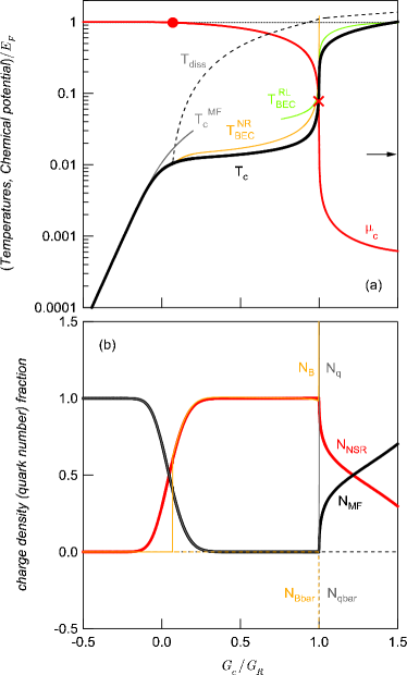
Figure 1: (a)  The critical temperature (chemical potential) $T_{c}$ ($\mu_{c}$) as a function of attractive coupling $G_{c}/G_{R}$. The dissociation temperature of pre-formed pair is also depicted by dashed line. (b)  The quark number fractions.

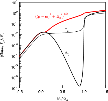
Figure 2: The zero temperature gap parameter $\Delta_{0}$, and $T_{c}$ as a function of $G_{R}^{-1}$. The mean field gap parameter $\Delta_{0}$ is calculated at $(\mu=\mu_{c},T=0)$. The physical gap in the single quark excitation at $T=0$, $\sqrt{\mathstrut\Delta_{0}^{2}+{\rm max.}(m-\mu_{c},0)^{2}}$, is also shown by the bold red line.

As $G_{c}/G_{R}$ grows, $T_{c}$ gradually deviates from the mean field result and for $G_{c}/G_{R}\mathrel{\mathchoice{\vbox{\offinterlineskip\halign{\hfil$\displaystyle#$\hfil\cr>\crcr\vskip 0.0pt\cr\sim\crcr}}}{\vbox{\offinterlineskip\halign{\hfil$\textstyle#$\hfil\cr>\crcr\vskip 0.0pt\cr\sim\crcr}}}{\vbox{\offinterlineskip\halign{\hfil$\scriptstyle#$\hfil\cr>\crcr\vskip 0.0pt\cr\sim\crcr}}}{\vbox{\offinterlineskip\halign{\hfil$\scriptscriptstyle#$\hfil\cr>\crcr\vskip 0.0pt\cr\sim\crcr}}}}0.07$ the bound state formation takes place and the system goes into the BEC regime. The bound state formation in medium $(k_{F}\neq 0)$ always takes place at a stronger coupling than $G_{c}/G_{R}=0$, the unitary coupling. This is because the Bethe-Salpeter kernel is smeared the Pauli-blocking effect at finite density. FIG. 3 also shows this fact. The bold line shows the half of boson mass $M_{B}(\mu_{c},T_{c})/2\equiv\mu_{c}$ while the thin line represents the half of antiboson mass $M_{\bar{B}}(\mu_{c},T_{c})/2$ as a function of $G_{R}$. We can clearly see that the antiboson forms prior to the formation of boson. The antiboson forms almost $G_{c}/G_{R}\sim 0$ where the bound state forms in vacuum, while boson does not form up to a little stronger attraction $G_{c}/G_{R}=0.07$; this means that the Pauli-blocking by on-shell fermions actually prevents the formation of boson.

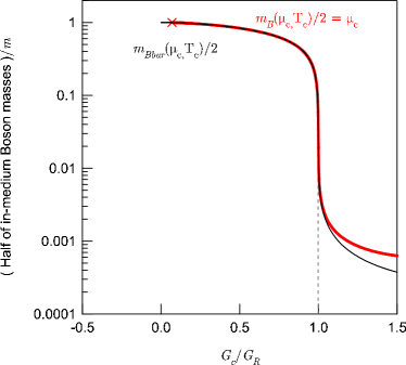
Figure 3: The in-medium boson and antiboson masses $(M_{B},M_{\bar{B}})$ as a function of attraction $G_{R}^{-1}$. The cross indicates the point $G_{c}/G_{R}\cong 0.07$ where the bound boson forms, i.e., $M_{B}(\mu_{c},T_{c})=2\mu_{c}=2m$ holds at this point.

In the BEC regime, the growth of $T_{c}$ as a function of $G_{c}/G_{R}$ is suppressed because the increase of attraction is mainly used to reduce the in-medium bound state mass. Because the in-medium boson mass changes, temperature does not saturate to the ideal BEC temperature of boson with mass $M_{B}=2m$ which is indicated by the arrow in the figure; this is in contrast to the nonrelativistic calculations nozieres ; melo93 ; Haussmann . $T_{c}$ in this region is well approximated by the nonrelativistic ideal BEC temperature ($T_{\rm BEC}^{\rm NR}$) of the boson with mass $2\mu_{c}$,

$$T_{\rm BEC}^{\rm NR}=k_{F}\frac{k_{F}}{\mu_{c}}\frac{1}{\pi^{1/3}}\left(\frac{1}{3\zeta_{2/3}}\right)^{2/3}.$$ (78)

This is shown by the thin orange line in figure (a). It is remarkable that this expression has no explicit dependence on $G_{R}$; there is only the implicit dependence on $G_{R}$ thorough $2\mu_{c}$, i.e., the in-medium boson mass. This fact expresses that the condensation in this regime has a rather kinematical origin. The factor $N_{c}-1$ in the above expression also indicates the condensation in this regime depends on the kinematical degrees of freedom; the factor comes from the fact there are $N_{c}$ fermions in the system while we have $d_{B}=N_{c}(N_{c}-1)/2$ bosons belonging to the $\bar{\bf 3}_{c}$ representation of SU$(3)$. This is in contrast to $T_{c}^{\rm MF}$ in the BCS region where we find no parametric dependence on $N_{c}$. It is also noteworthy that the universal relation $T_{c}/\Delta_{0}=0.567$ is significantly violated as seen in FIG. 2; $T_{c}/\Delta_{0}$ grows up to $\sim 10^{5}$. However, the physical gap in the single quark excitation at $T=0$, $\sqrt{\mathstrut\Delta_{0}^{2}+\theta(m-\mu_{c})(m-\mu_{c})^{2}}$, is always comparable to $T_{c}$.

As the attraction, $G_{c}/G_{R}$, is further increased beyond the unity, the system goes into the RBEC phase where $T_{c}$ exceeds the in-medium boson mass $2\mu_{c}$. The critical temperature in this regime is well approximated by the ideal BEC temperature $T_{\rm BEC}^{\rm RL}$ of a relativistic bose gas:

$$T_{\rm BEC}^{\rm RL}=\frac{k_{F}}{\pi}\sqrt{\mathstrut\frac{k_{F}}{2\mu_{c}}}.$$ (79)

Because the in-medium boson mass is smaller than the critical temperature, there are a lot of bosons and antibosons as shown in Fig. 1 (b). We notice that unlike the ideal BEC of the elementary boson gas kapusta , there are a lot of (anti)fermions as well as (anti)bosons in the RBEC regime. This is the characteristic feature of the composite boson system, where there exists the competition between free energy and entropy; two fermion state is more favorable than one boson state in terms of entropy, but is less favorable in terms of free energy. This consists one reason why we find a relatively large deviation between the real $T_{c}$ and $T_{\rm BEC}^{\rm RL}$ in the RBEC regime.

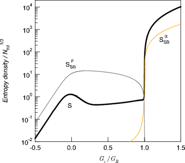
Figure 4: The entropy par quark number charge as a function of $G_{R}^{-1}$. $S_{F}=N_{c}N_{f}(\frac{\mu_{c}^{2}T_{c}}{3}+\frac{7\pi^{2}T_{c}^{3}}{45})$ is the entropy for free massless quark gas and $S_{B}=N_{c}(N_{c}-1)\frac{2\pi^{2}T_{c}^{3}}{45}$ is the Stephan-Boltzmann entropy for $N_{c}(N_{c}-1)/2$-“flavored” boson gas.

To confirm the above-discussed physical picture, we show in FIG. 4, how the total entropy behaves going from the BCS to the RBEC. We can see that the entropy in the BCS regime is suppressed from the free massless fermion result because of the pairing correlation and finite mass. When the system goes into the BEC region, the entropy takes a nearly constant value. This is because the increase of the coupling mainly affects the internal structure (the binding) of the boson and the kinetic degrees of freedom controlling $T_{c}$ does not change. When the system goes into the RBEC phase, the entropy rapidly increases because there appear a lot of kinetic degrees of freedom, $\{q,\bar{q},B,\bar{B}\}$. Since plenty of $(q,\bar{q})$ are present in addition to $(B,\bar{B})$, the Stephan-Boltzmann entropy for the ideal bose gas underestimates the total entropy.

III.2 Character change of Cooper pair and Deformation of Fermi surface

To obtain a more intuitive insight into the three regions, we here study the character change of Cooper pair wavefunction, the spectral density, and fermion occupation numbers. In FIG. 5, we show the spectral density [(a); left panel], the Cooper pair wavefunction [(b); middle panel], and the (anti)fermion occupancy [(c); right panel]. From top to bottom, the renormalized coupling grows as $G_{c}/G_{R}=-0.35$ (BCS), $G_{c}/G_{R}=0.5$ (BEC), and $G_{c}/G_{R}=1.35$ (RBEC).

We first discuss how the spectral density evolves from the weak coupling BCS to the strong coupling RBEC phase. Figure (a1) shows the spectral density $m^{2}\rho^{\rm Ren}_{\mu_{c},T_{c}}(\omega,\mbox{\boldmath$0$})$ in the BCS phase. We can see that the Thouless “zero” of the inverse susceptibility at $\omega=0$ is located above the 2-particle “decay” (and 2-hole “absorption”) continuum threshold, i.e., $0>2m-2\mu_{c}$. This means that the pair fluctuation with finite momentum in the BCS state decays into two quarks. We confirm this later by constructing the low energy effective theory for the fluctuating pair field. FIG. 5 (b1) shows the spectral density in the BEC state. In contrast to the BCS case, the Thouless singularity at $\omega=0$ is realized as a bound state (boson) isolated pole. This is because $\omega=0$ is located below the 2-particle continuum, i.e., $0<2m-2\mu_{c}$. There exists another singularity in the region $\omega+2\mu<0$ corresponding to the in-medium antiboson pole. We note, however, that the thermodynamic quantity should be expressed by the integral of the combination $\tilde{f}_{B}(\omega)\times\rho_{\mu_{c},T_{c}}^{\rm Ren}(\omega,\mbox{\boldmath$P$})$, so the antiboson pole gives only an exponentially suppressed contribution to the thermodynamic quantities like entropy, heat capacity, etc. If we go higher temperature $T>T_{c}$ with fixing $\mu=\mu_{c}$, then the boson pole gradually shifts to higher $\omega$ because the bound state dissociates thermally (see the thin orange line in the figure). As we increase the temperature, the pole eventually gets absorbed into the 2-particle continuum at the dissociation temperature $T=T_{\rm diss}$. The spectral density at $T=T_{\rm diss}$ is depicted in the figure by the thin red line. Interestingly enough, the antiboson pole still survives at this temperature; this is attributed to the fact that the Pauli-blocking effect is less significant in the antiboson sector than in the boson sector. Finally, we show the spectral density $m^{2}\rho^{\rm Ren}_{\mu_{c},T_{c}}(\omega,P=m)$ in the RBEC phase in FIG. 5 (c1). Because $\mu_{c}\ll T_{c}$ in this regime, the spectral function is almost antisymmetric with respect to $\omega\leftrightarrow-\omega$. In the region $-P<\omega+2\mu<P$, the decay of the pair fluctuating mode by absorbing thermally excited antiquarks (the Landau damping process) is kinematically allowed. Because of this, the spectral density takes non-zero value in this region. In the RBEC phase, the temperature is so high ($T_{c}\gg\mu_{c}$) that this Landau damping process gives a significant contribution to the unstable content $N_{\rm un}$ in $N_{\rm NSR}(\mu_{c},T_{c})$. This is one of the characteristic features in the relativistic fermion system.

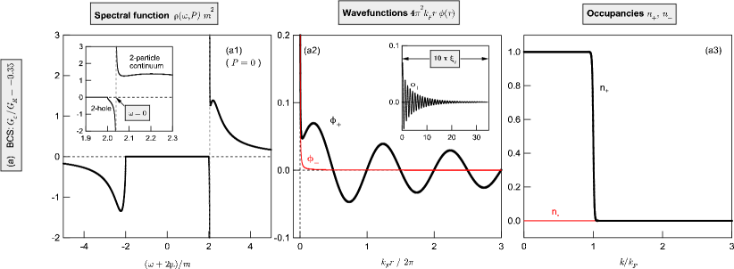
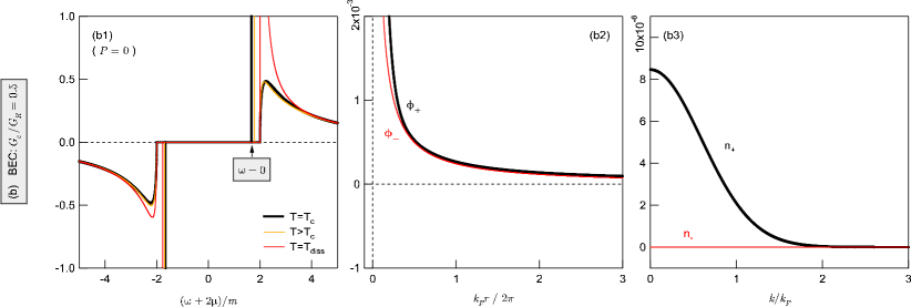
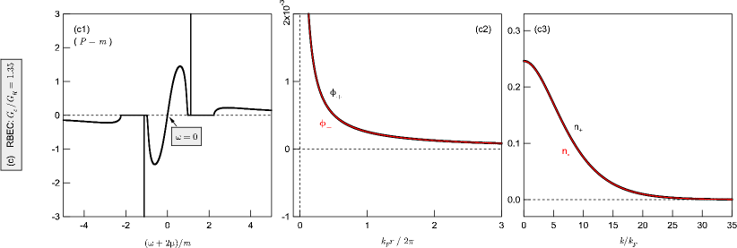
Figure 5: The spectral density as a function of $\omega+2\mu$ (left panel), wavefunctions in the real space (middle), and the occupation numbers as a function of momentum $k$ (right panel). From top to bottom, the attractive coupling increases as $G_{c}/G_{R}=-0.35$ (a), $G_{c}/G_{R}=0.5$ (b), and $G_{c}/G_{R}=1.35$ (c); the system evolves as the BCS (a), the BEC (b), and the RBEC state (c). The inset of (a1) is an enlargement near $\omega=0$, and the inset of (a2) shows the behaviour of the wavefunction at large length scale.

Next we study how the internal structure of the Cooper pair changes throughout the crossover. Let us first begin with the definition of the Cooper pair “wavefunction”. We may define it from the expression of the correlation functions for $T\leq T_{c}$ Abuki:2003ut :

$$\begin{array}[]{rcl}&&\left\langle q^{a}_{i}(0,\mbox{\boldmath$x$})q^{b}_{j}(-i0^{-},\mbox{\boldmath$y$})\right\rangle\\[8.61108pt] &=&+(\tau_{2}\lambda_{2})^{ab}_{ij}\int\frac{d\mathstrut\mbox{\scriptsize{\boldmath$q$}}\mathstrut}{(2\pi)^{3}}e^{i\mathstrut\mbox{\scriptsize{\boldmath$q$}}\mathstrut\cdot(\mathstrut\mbox{\scriptsize{\boldmath$x$}}\mathstrut-\mathstrut\mbox{\scriptsize{\boldmath$y$}}\mathstrut)}\phi_{+}(q)\Delta\gamma_{5}C\Lambda_{+}(\hat{q})\\[8.61108pt] &&+(\tau_{2}\lambda_{2})^{ab}_{ij}\int\frac{d\mathstrut\mbox{\scriptsize{\boldmath$q$}}\mathstrut}{(2\pi)^{3}}e^{i\mathstrut\mbox{\scriptsize{\boldmath$q$}}\mathstrut\cdot(\mathstrut\mbox{\scriptsize{\boldmath$x$}}\mathstrut-\mathstrut\mbox{\scriptsize{\boldmath$y$}}\mathstrut)}\phi_{-}(q)\Delta\gamma_{5}C\Lambda_{-}(\hat{q}),\\[8.61108pt] \end{array}$$ (80)

where the quark-quark pair wavefunction $\phi_{+}$ and the antiquark-antiquark pair wavefunction $\phi_{-}$ are defined by

$$\phi_{\pm}(q)=\tanh\left(\frac{\epsilon_{q\pm}}{2T}\right)\frac{1}{2\epsilon_{q\pm}},$$ (81)

$\epsilon_{q\pm}\equiv\sqrt{\mathstrut(E_{q}\mp\mu)^{2}+\Delta^{2}}$ is the quasi-(anti)quark energy. These wavefunction in $q$-space can be Fourier-transformed to the real space:

$$\phi_{\pm}(r)=\frac{1}{2\pi^{2}r}\int_{0}^{\infty}dq\frac{q\sin(qr)}{2\epsilon_{q\pm}}\tanh\left(\frac{\epsilon_{q\pm}}{2T}\right).$$ (82)

Unlike the nonrelativistic situation, this integral does not converge even for $r\neq 0$; the integrand oscillates with $\sin(qr)$ as $q\to\infty$. Evaluating the oscillating integral by the sharp cutoff $\Lambda$ is inappropriate, and therefore we take the following prescription to regulate this integral. By integrating by parts, we obtain

$$\begin{array}[]{rcl}\phi_{\pm}(r)&=&-\frac{1}{2\pi^{2}r^{2}}\left[\frac{q\cos(qr)}{2\epsilon_{q\pm}}\tanh\left(\frac{\epsilon_{q\pm}}{2T}\right)\right]_{\scriptsize q\to\infty}\\ &&+\frac{1}{2\pi^{2}r^{2}}\int_{0}^{\infty}dq\cos(qr)\frac{\partial}{\partial q}\left[\frac{q}{2\epsilon_{q\pm}}\tanh\left(\frac{\epsilon_{q\pm}}{2T}\right)\right].\\[8.61108pt] \end{array}$$ (83)

The second term is conversing while there remains a oscillating uncertainty in the first term. However, if we adopted the smooth cutoff scheme, the first term should vanish. Thus we may define the second term of Eq. (83) as the regularized Cooper pair wavefunction:

$$\begin{array}[]{rcl}\phi_{\pm}(r)&=&+\frac{1}{2\pi^{2}r^{2}}\int_{0}^{\infty}dq\cos(qr)\frac{\partial}{\partial q}\left[\frac{q}{2\epsilon_{q\pm}}\tanh\left(\frac{\epsilon_{q\pm}}{2T}\right)\right].\\[8.61108pt] \end{array}$$ (84)

Using the regularized Cooper pair function, we can evaluate the Cooper pair size (Coherence length) melo97 ; Abuki:2001be :

$$\xi_{c}^{2}(T)=\frac{\langle\phi_{+}(\mbox{\boldmath$r$})|\mbox{\boldmath$r$}^{2}\phi_{+}(\mbox{\boldmath$r$})\rangle}{\langle\phi_{+}(\mbox{\boldmath$r$})|\phi_{+}(\mbox{\boldmath$r$})\rangle}=-\frac{\langle\phi_{+}(\mbox{\boldmath$q$})|\nabla_{\mathstrut\mbox{\scriptsize{\boldmath$q$}}\mathstrut}^{2}\phi_{+}(\mbox{\boldmath$q$})\rangle}{\langle\phi_{+}(\mbox{\boldmath$q$})|\phi_{+}(\mbox{\boldmath$q$})\rangle_{\scriptsize\Lambda}}.$$ (85)

FIG. 5(b1) shows the Cooper pair wavefunctions $4\pi^{2}k_{F}r\phi_{\pm}(r)$ at $T=T_{c}$ in the BCS phase ($G_{c}/G_{R}=-0.35$). We can see that the wave function $\phi_{+}(r)$ oscillates with a period $\sim 2\pi/k_{F}$ and decays exponentially ${\rm e}^{-\frac{r}{\pi\xi_{p}}}$ with the Pippard length

$$\xi_{p}=\frac{k_{F}}{E_{F}}\frac{1}{\pi\Delta_{0}}.$$ (86)

$\Delta_{0}\sim 1.764T_{c}$ is the gap at zero temperature Abuki:2001be . The Pippard length is the weak coupling (BCS) approximation of the pair size at $T=0$, i.e., $\xi_{p}\cong\xi_{c}(T=0)$ in the BCS regime. The inset of FIG. 5(1b) shows the magnitude of wavefunction actually decays exponentially at large scale $r>\xi_{c}\equiv\xi_{c}(T_{c})$; note that the pair size is robust against the increase in temperature, $\xi_{c}(T_{c})\sim\xi_{c}(T=0)$ Abuki:2003ut . Also it is consistent with Abuki:2003ut that the antiquark pair correlation is negligible in the BCS regime. How this situation changes as the coupling grows? FIG. 5(2b) shows the wavefunctions $4\pi^{2}k_{F}r\phi_{\pm}(r)$ in the BEC region. We first notice that the wavefunction $\phi_{+}(r)$ has no oscillating structure like that in the BCS. This is easily anticipated by the fact that the in-medium bound state forms in this regime and that the bound state in the $s$-wave channel is unique; so the “wavefunction” should not have any nodes in the real space nozieres . This is in contrast to Matsuzaki:1999ww ; Abuki:2001be where the pair structure at low density still has a oscillating structure; this fact shows that the in-medium bound state is not formed there. In this region, the Pippard length is not a good approximation of the pair size. In this regime, the pair size is roughly approximated by the $s$-wave scattering length $a_{s}$. This is because, neglecting matter effects, the bound state wavefunction in the C.M. frame should behave as $\sim e^{-r/\sqrt{\mathstrut 2}a_{s}}$ as $r\to\infty$. We will confirm these later. It is also notable that there is a slight deviation in the wavefunctions $\phi_{+}(r)$ and $\phi_{-}(r)$ in this regime reflecting the explicit breaking of charge conjugation by finite $\mu$. In the RBEC phase, however, $\phi_{+}$ and $\phi_{-}$ show almost the same behaviour because of $\mu_{c}\ll T_{c}$ (see FIG. 5(3b)).

Finally, we discuss how the Fermi surface is destructed when the attraction is increased. To see this, we have plotted the occupation numbers in FIG. 5(c1) $\sim$ (c3). From these figures, we can clearly see that the Fermi surface gets significantly broken once the in-medium bound state have appeared in the spectrum. Baryon number carrier in the BEC regime is almost the bosonic degrees of freedom as we can see also from FIG. 1(b). In the RBEC phase, the temperature is high $T_{c}\gg\mu_{c}$, and thus fermions are again thermally active for the entropic reason we noted in the previous section. Also, the quark-antiquark asymmetry is small because of ($\mu_{c}\ll T_{c}$).

IV The evolution of the soft mode dynamics

In this section, we construct the low energy effective theory for the pair fluctuation transport and study how the static and dynamic nature of the soft mode evolves as the system goes from the weak coupling BCS to the RBEC. In the context of a nonrelativistic BCS superconductor, the effective theories for the fluctuating pair field both for (i) near $T_{c}$ and (ii) near $T=0$ were derived in Abrahams where a diffusion type equation was found above $T_{c}$. The dynamics of the spece-time variation of fluctuation in color superconductivity above $T_{c}$ was first investigated in Kitazawa:2005vr where the authors found a damped-oscillation type equation within the linear level. The effect of fluctuating pair fields to the specific heat was also investigated in Voskresensky:2004jp starting with the ansatz that the pair fluctuation is a propagating mode with a relativistic dispersion. By extending Kitazawa:2005vr along with the nonrelativistic calculations melo93 ; Abrahams , we will find the following three points: (i) The pair fluctuation in the BCS regime is a diffusive mode but with small propagating piece melo93 ; Kitazawa:2005vr . (ii) In the BEC regime, the fluctuating pair field is of a propagating mode but with a nonrelativistic dispersion melo93 . (iii) The fluctuation is also propagating in the RBEC region and the relativistic (an almost linear) dispersion is realized in a wide kinematical region.

Let us start our analysis with first looking at the static part of the fluctuation. In the context of color superconductivity, this was first done in Iida:2000ha in the weak coupling BCS regime. The long wavelength expansion of the pair susceptibility near $T=T_{c}$ leads to

$$\left[\Gamma^{\rm Ren}_{\mu,T}(0,\mbox{\boldmath$P$})\right]^{-1}=a_{0}\frac{T-T_{c}}{T_{c}}+\frac{c}{4m}\mbox{\boldmath$P$}^{2}+\cdots,$$ (87)

where the mass-squared parameter $a_{0}$ and the stiffness parameter (or diffusion constant) $c$ are defined by

$$\begin{array}[]{rcl}a_{0}&=&T_{c}\frac{\partial}{\partial T}\left[\Gamma^{\rm Ren}_{\mu,T}(0,\mbox{\boldmath$0$})\right]^{-1}\big{|}_{T=T_{c}},\\[8.61108pt] c&=&4m\frac{\partial}{\partial\mathstrut\mbox{\scriptsize{\boldmath$P$}}\mathstrut^{2}}\left[\Gamma^{\rm Ren}_{\mu,T}(0,\mbox{\boldmath$P$})\right]^{-1}\big{|}_{\mathstrut\mbox{\scriptsize{\boldmath$P$}}\mathstrut=\mathstrut\mbox{\scriptsize{\boldmath$0$}}\mathstrut}.\\[4.30554pt] \end{array}$$ (88)

The explicit calculation yields Kitazawa :

$$\begin{array}[]{rcll}a_{0}&=&\frac{1}{T_{c}}\int\frac{d\mathstrut\mbox{\scriptsize{\boldmath$q$}}\mathstrut}{(2\pi)^{3}}\biggl{[}\frac{1}{\cosh^{2}\left(\frac{E_{q}-\mu}{2T_{c}}\right)}+\frac{1}{\cosh^{2}\left(\frac{E_{q}+\mu}{2T_{c}}\right)}\biggl{]},&\\[8.61108pt] \frac{c}{4m}&=&\int\frac{d\mathstrut\mbox{\scriptsize{\boldmath$q$}}\mathstrut}{(2\pi)^{3}}\left[\frac{q^{2}{\rm sech}^{2}\left(\frac{E_{q}-\mu}{2T_{c}}\right)\tanh\left(\frac{E_{q}-\mu}{2T_{c}}\right)}{24T_{c}^{2}E_{q}^{2}(E_{q}-\mu)}+(\mu\leftrightarrow-\mu)\right]&\quad\cdots{\mathcal{O}}\big{(}\frac{\mu^{2}}{T_{c}^{2}}\big{)}\\[8.61108pt] &&-{\mathcal{P}}\int\frac{d\mathstrut\mbox{\scriptsize{\boldmath$q$}}\mathstrut}{(2\pi)^{3}}\left[\frac{(2E_{q}^{2}+m^{2}){\rm sech}^{2}\left(\frac{E_{q}-\mu}{2T_{c}}\right)}{24T_{c}E_{q}^{3}(E_{q}-\mu)}+(\mu\leftrightarrow-\mu)\right]&\quad\cdots{\mathcal{O}}\big{(}\frac{\mu}{T_{c}}\big{)}\\[8.61108pt] &&-{\mathcal{P}}\int\frac{d\mathstrut\mbox{\scriptsize{\boldmath$q$}}\mathstrut}{(2\pi)^{3}}\left[\frac{(2E_{q}^{2}+m^{2})(2E_{q}-\mu)\tanh\left(\frac{E_{q}-\mu}{2T_{c}}\right)}{6\mu E_{q}^{3}(E_{q}-\mu)^{2}}+(\mu\leftrightarrow-\mu)\right]&\quad\cdots{\mathcal{O}}\big{(}1\big{)}.\\[4.30554pt] \end{array}$$ (89)

We note that $a_{0}$ has no UV divergence, while $c$ still has a logarithmic divergence in the last term in Eq. (89) which is sub-sub-dominant in the $(\mu/T_{c})$-expansion; accordingly, the integral is conversing in the weak coupling limit, while it is not in the strong coupling. We may simply regularize the divergence by sharp cutoff $\Lambda$.

In the extremely weak coupling BCS regime where $\mu_{c}\gg T_{c}$, we can derive some analytic approximations. First, we may safely ignore the contribution from antiquarks, and can replace the momentum integral $\int\frac{d\mathstrut\mbox{\scriptsize{\boldmath$q$}}\mathstrut}{(2\pi)^{3}}$ by $N_{0}\int_{-\infty}^{\infty}dE_{q}$ with $N_{0}=\frac{\mu^{2}}{2\pi^{2}}$ being the density of state at $E_{q}=\mu$. We then arrive at the approximations:

$$a_{0}^{\rm BCS}=4N_{0},\quad\frac{c^{\rm BCS}}{4m}=\frac{7\zeta(3)k_{F}^{2}}{12\pi^{2}\mu^{2}T_{c}^{2}}N_{0}.$$ (90)

Because $\Gamma^{\rm Ren}_{\mu,T}(0,\mbox{\boldmath$P$})\sim\frac{1}{\mathstrut\mbox{\scriptsize{\boldmath$P$}}\mathstrut^{2}+\frac{4ma_{0}}{c}t_{r}}$ near $T=T_{c}$, with $t_{r}=\frac{T-T_{c}}{T_{c}}$ being the reduced temperature, the static disturbance of the system restores at the “healing” length

$$\xi_{\rm GL}t_{r}^{-1/2},$$ (91)

where the Ginzburg-Landau (GL) coherence length $\xi_{\rm GL}$ is defined by

$$\xi_{\rm GL}\equiv\sqrt{\mathstrut\frac{c}{4ma_{0}}}.$$ (92)

The healing length diverges as $T\to T_{c}+0$ as a consequence of the second order phase transition. In the weak coupling BCS regime ($\mu\gg T_{c}$), the GL coherence length is approximated by (substituting Eq. (90) into Eq. (92)),

$$\begin{array}[]{rcl}\xi_{\rm GL}^{\rm BCS}&=&\frac{k_{F}}{E_{F}}\frac{\sqrt{\mathstrut 21\zeta(3)}}{12T_{c}}\cong 0.739\xi_{p},\\[4.30554pt] \end{array}$$ (93)

a well-known relation between the Pippard length and the GL healing length in the nonrelativistic BCS theory.

We now look at the dynamic part of the problem. One must be careful in performing the low frequency expansion of the dynamic pair susceptibility near $T_{c}$ because there arises a spectral singularity in the kinematical region $\omega/P<v_{F}$ once the system goes below $T_{c}$ Abrahams ; $v_{F}$ is the Fermi velocity of quasi-quarks. This singularity is attributed to the local absorption (or emission) of the Goldstone mode (phonon) by thermally active quasi-quarks. A simple expansion is allowed only for the region near the critical temperature $T\sim T_{c}$ where the gap is small $\omega\gg\Delta(T)$. In such region, we can naively perform the low frequency expansion Abrahams as

$$\left[\Gamma^{\rm Ren}_{\mu,T}(\omega,\mbox{\boldmath$0$})\right]^{-1}=-d\omega-d_{2}\omega^{2}+\cdots,$$ (94)

where $d$ and $d_{2}$ are defined by

$$\begin{array}[]{rcl}d&=&-\frac{\partial}{\partial\omega}\left[\Gamma^{\rm Ren}_{\mu,T_{c}}(\omega,\mbox{\boldmath$0$})\right]^{-1}\big{|}_{\omega=0},\\[8.61108pt] d_{2}&=&-\frac{1}{2}\frac{\partial^{2}}{\partial\omega^{2}}\left[\Gamma^{\rm Ren}_{\mu,T_{c}}(\omega,\mbox{\boldmath$0$})\right]^{-1}\big{|}_{\omega=0}.\\[4.30554pt] \end{array}$$ (95)

These quantities are complex in the BCS region $(\mu>m)$, while they become real in the BEC region $(\mu<m)$ because the imaginary part of the dynamic pair susceptibility looks like

$$\begin{array}[]{rcl}{\rm Im}\left[\Gamma^{\rm Ren}_{\mu,T_{c}}(\omega,\mbox{\boldmath$0$})\right]^{-1}&=&-\theta(\omega+2\mu>2m)\\[8.61108pt] &&\times\frac{(\omega+2\mu)\sqrt{\mathstrut(\omega+2\mu)^{2}-4m^{2}}\tanh\left(\frac{\omega}{4T_{c}}\right)}{4\pi}.\end{array}$$ (96)

Further explicit calculation leads

$$\begin{array}[]{rcl}d&=&{\mathcal{P}}\int\frac{d\mathstrut\mbox{\scriptsize{\boldmath$q$}}\mathstrut}{(2\pi)^{3}}\left[\frac{\tanh\left(\frac{E_{q}-\mu}{2T_{c}}\right)}{(E_{q}-\mu)^{2}}-\frac{\tanh\left(\frac{E_{q}+\mu}{2T_{c}}\right)}{(E_{q}+\mu)^{2}}\right]\\[8.61108pt] &&+i\theta(\mu>m)\frac{\mu\sqrt{\mathstrut\mu^{2}-m^{2}}}{4\pi T_{c}},\\[8.61108pt] d_{2}&=&{\mathcal{P}}\frac{1}{2}\int\frac{d\mathstrut\mbox{\scriptsize{\boldmath$q$}}\mathstrut}{(2\pi)^{3}}\left[\frac{\tanh\left(\frac{E_{q}-\mu}{2T_{c}}\right)}{(E_{q}-\mu)^{3}}+\frac{\tanh\left(\frac{E_{q}+\mu}{2T_{c}}\right)}{(E_{q}+\mu)^{3}}\right]\\[8.61108pt] &&+i\theta(\mu>m)\frac{2\mu^{2}-m^{2}}{8\pi T_{c}\sqrt{\mathstrut\mu^{2}-m^{2}}}.\\[4.30554pt] \end{array}$$ (97)

The weak coupling $(\mu\gg T_{c})$ approximation again applies both to $d$ and $d_{2}$ yielding the following analytic results.

$$\begin{array}[]{rcl}d^{\rm BCS}&=&iN_{0}\frac{\pi}{2T_{c}},\\[8.61108pt] d^{\rm BCS}_{2}&=&-N_{0}\frac{7\zeta(3)}{4\pi^{2}T_{c}^{2}}+iN_{0}\left(\frac{2\mu^{2}-m^{2}}{\mu^{2}-m^{2}}\right)\frac{\pi}{4\mu T_{c}}.\end{array}$$ (98)

Note that $d^{\rm BCS}$ is pure imaginary reflecting the particle-hole symmetry in the weak coupling limit Abrahams . This means that, to this order, the pair fluctuation obeys a diffusion-type equation in the BCS phase Abrahams ; melo93 . In reality, there is a finite real part which is an order $(T_{c}/\mu)$ suppressed from the imaginary part though. This real part arises from a particle-hole asymmetry and adds a small propagating nature to the soft mode; as a consequence, the fluctuation in the BCS region becomes a damped-oscillation mode Kitazawa:2005vr or an overdamped mode melo93 . The coefficient of second-time derivative, $d_{2}$, is also non-vanishing. This is another source of a propagating nature of the soft mode.

So far, we have concentrated on the kinematical aspect of the pair fluctuation. It is sometimes important to know about the interaction between soft modes to investigate the transport properties of system. For example, the shear viscosity is proportional to the mean free path $(l_{\rm MFP})$ of soft modes in the classical level. This requires an information about the collision between soft modes. We here look at the interaction between soft modes.

The partition function is factorized as $Z_{0}e^{-S_{\rm eff}}$ where $Z_{0}$ is the partition function for free quark gas, and $S_{\rm eff}$ is the effective action for fluctuation. We need to go beyond the gaussian approximation for $S_{\rm eff}$. Up to the quartic order in $\Delta$, we have

$$\begin{array}[]{rcl}S_{\rm eff}[\Delta,\Delta^{*}]&=&\displaystyle T\sum_{N,\eta}\int\frac{d\mbox{\boldmath$P$}}{(2\pi)^{3}}\left[\Gamma^{\rm Ren}_{\mu,T}(i\Omega_{N},\mbox{\boldmath$P$})\right]^{-1}|\Delta_{\eta}(i\Omega_{N},\mbox{\boldmath$P$})|^{2}\\[8.61108pt] &&\displaystyle+\frac{1}{4}\sum_{\eta,\xi}\sum_{1,2,3}b_{1,2,3}\Delta_{\eta}(1)\Delta_{\eta}(2)^{*}\Delta_{\xi}(3)\Delta_{\xi}^{*}(1-2+3)\\[8.61108pt] &&\displaystyle+\frac{1}{4}\sum_{\eta,\xi}\sum_{1,2,3}b^{{}^{\prime}}_{1,2,3}\Delta_{\eta}(1)\Delta_{\xi}(2)^{*}\Delta_{\xi}(3)\Delta_{\eta}^{*}(1-2+3).\\[4.30554pt] \end{array}$$ (99)

Here numbers $\{1,2,3\}$ are labeling sets of frequency and momentum $\{(i\Omega_{N1},\mbox{\boldmath$P$}_{1}),(i\Omega_{N2},\mbox{\boldmath$P$}_{2}),(i\Omega_{N3},\mbox{\boldmath$P$}_{3})\}$, and $\sum_{1,2,3}$ is a shorthand of $T^{3}\sum_{N_{1},N_{2},N_{3}}\int\frac{d\mathstrut\mbox{\scriptsize{\boldmath$P$}}\mathstrut_{1}}{(2\pi)^{3}}\frac{d\mathstrut\mbox{\scriptsize{\boldmath$P$}}\mathstrut_{2}}{(2\pi)^{3}}\frac{d\mathstrut\mbox{\scriptsize{\boldmath$P$}}\mathstrut_{3}}{(2\pi)^{3}}$. To derive the low energy effective action, we set $\Delta_{\eta}(i\Omega_{N})=0$ for $N=\pm 1,\pm 2,\cdots$, and only consider the fluctuation mode with the lowest Matsubara frequency. Thus $\Delta$ has no dependence on $\tau$. Then the quadratic term of $S_{\rm eff}$ is casted into the form $\beta\int d\mbox{\boldmath$x$}f_{\rm eff}^{\rm kin}(\Delta(x),\Delta^{*}(x))$ with the kinetic part of the local effective (classical) free energy density defined by

$$\begin{array}[]{rcl}f_{\rm eff}^{\rm kin}&=&\sum_{\eta}\Delta_{\eta}(\mbox{\boldmath$x$})^{*}\left[a_{T}-\frac{c}{4m}\nabla_{\mathstrut\mbox{\scriptsize{\boldmath$x$}}\mathstrut}^{2}+\cdots\right]\Delta_{\eta}(\mbox{\boldmath$x$})\\[8.61108pt] &=&\sum_{\eta}\left[a_{T}|\Delta_{\eta}(\mbox{\boldmath$x$})|^{2}+\frac{c}{4m}|\nabla_{\mathstrut\mbox{\scriptsize{\boldmath$x$}}\mathstrut}\Delta_{\eta}(\mbox{\boldmath$x$})|^{2}\right].\end{array}$$ (100)

$a_{T}\equiv a_{0}\frac{T-T_{c}}{T_{c}}$ is the mass parameter and $c$ is the diffusion constant introduced before. The quartic term also can be written in the form $\beta\int{d\mbox{\boldmath$x$}}f^{\rm int}_{\rm eff}(\Delta,\Delta^{*})$ with

$$\begin{array}[]{rcl}f_{\rm eff}^{\rm int}&=&\sum_{\eta,\xi}\frac{b_{0}}{2}|\Delta_{\eta}(\mbox{\boldmath$x$})|^{2}|\Delta_{\xi}(\mbox{\boldmath$x$})|^{2}.\end{array}$$ (101)

where $b_{0}=b_{0,0,0}=b^{{}^{\prime}}_{0,0,0}$ is calculated as

$$\begin{array}[]{rcl}b_{0}&=&\displaystyle 2T\sum_{n}\int\frac{d\mbox{\boldmath$q$}}{(2\pi)^{3}}\mbox{tr}\left[S_{F}(i\omega_{n},\mbox{\boldmath$q$})S_{F}(-i\omega_{n},-\mbox{\boldmath$q$})S_{F}(i\omega_{n},\mbox{\boldmath$q$})S_{F}(-i\omega_{n},-\mbox{\boldmath$q$})\right]\\[8.61108pt] &=&\displaystyle\frac{1}{T}\int\frac{d\mbox{\boldmath$q$}}{(2\pi)^{3}}\Biggl{[}\frac{-(E_{q}-\mu)+T\sinh\big{(}\frac{E_{q}-\mu}{T}\big{)}}{(E_{q}-\mu)^{3}\big{[}1+\cosh\big{(}\frac{E_{q}-\mu}{T}\big{)}\big{]}}+\frac{-(E_{q}+\mu)+T\sinh\big{(}\frac{E_{q}+\mu}{T}\big{)}}{(E_{q}+\mu)^{3}\big{[}1+\cosh\big{(}\frac{E_{q}+\mu}{T}\big{)}\big{]}}\Biggl{]}\end{array}$$ (102)

To derive this, we have taken care the lowest term omitting the gradient terms. This corresponds to the soft limit of the two body scattering where all the incoming and outgoing momenta vanish. The weak coupling BCS ($\mu\gg T_{c}$) approximation again applies to $b_{0}$ resulting in

$$b_{0}^{\rm BCS}=N_{0}\frac{7\zeta(3)}{2\pi^{2}T_{c}^{2}}.$$ (103)

Collecting all the above results, we arrive at the following expression for the local (but coarse-grained) Ginzburg-Landau (GL) free energy functional ($F_{\rm eff}=\int d{\mbox{\boldmath$x$}}(f_{\rm eff}^{\rm kin}+f_{\rm eff}^{\rm int})$) which describes the long wavelength (static) excitation of soft mode:

$$\begin{array}[]{rcl}F_{\rm eff}[\Delta,\Delta^{*}]&=&\int d\mbox{\boldmath$x$}\left[\sum_{\eta}\left[a_{T}|\Delta_{\eta}(\mbox{\boldmath$x$})|^{2}+\frac{c}{4m}|\nabla_{\mathstrut\mbox{\scriptsize{\boldmath$x$}}\mathstrut}\Delta_{\eta}(\mbox{\boldmath$x$})|^{2}\right]+\sum_{\eta,\xi}\frac{b}{2}|\Delta_{\eta}(\mbox{\boldmath$x$})|^{2}|\Delta_{\xi}(\mbox{\boldmath$x$})|^{2}\right].\\[4.30554pt] \end{array}$$ (104)

On the other hand, we have already derived the time dependence of the excitation at long time scale. Combining the nonlinear term in $\Delta(t,x)$, we obtain the following dynamic equation for the fluctuation transport:

$$\left[-id\partial_{t}+d_{2}\partial_{t}^{2}+a_{T}-\frac{c}{4m}\nabla_{\mathstrut\mbox{\scriptsize{\boldmath$x$}}\mathstrut}^{2}+b_{0}\sum_{\xi}|\Delta_{\xi}(t,\mbox{\boldmath$x$})|^{2}\right]\Delta_{\eta}(t,\mbox{\boldmath$x$})=0.$$ (105)

It can be written in the compact and familiar form:

$$\left[-id\partial_{t}+d_{2}\partial_{t}^{2}\right]\Delta_{\eta}(t,\mbox{\boldmath$x$})=-\frac{\delta F_{\rm eff}[\Delta,\Delta^{*}]}{\delta\Delta^{*}_{\eta}(t,\mbox{\boldmath$x$})}.$$ (106)

As for extremely low frequency modes with $(\omega\ll{\rm min.}\,(T_{c},|m-\mu|))$, we may simply ignore the second term (including $d_{2}$) in the left hand side of the above equation.

In the BCS regime, $d$ is imaginary dominant and is pure imaginary in the weak coupling limit as shown in Eq. (98). In this regime, Eq. (106) describes how the fluctuation about the thermal equilibrium relaxes; the thermodynamic restoring force to the equilibrium is then given by $-\frac{1}{d^{\rm BCS}}\frac{\delta F_{\rm eff}[\Delta,\Delta^{*}]}{\delta\Delta^{*}_{\eta}(\mbox{\boldmath$x$})}$. By rescaling the field by $\Psi(t,\mbox{\boldmath$x$})=\sqrt{\mathstrut c}\Delta(t,\mbox{\boldmath$x$})$, we find the standard expression for the time-dependent Ginzburg-Landau (TDGL) equation in the BCS regime:

$$\left[\frac{{\rm Im}\,d}{c}\partial_{t}+\frac{a_{T}}{c}-\frac{\nabla_{\mathstrut\mbox{\scriptsize{\boldmath$x$}}\mathstrut}^{2}}{4m}+\frac{b_{0}}{c^{2}}\sum_{\xi}|\Psi_{\xi}(t,\mbox{\boldmath$x$})|^{2}\right]\Psi_{\eta}(t,\mbox{\boldmath$x$})=0.$$ (107)

The pair fluctuation is diffusive as in the nonrelativistic case Abrahams ; melo93 ; ignoring the nonlinear term, the mode with wavenumber $k$ decays exponentially

$$\Psi_{\xi}(t,k)\sim e^{-t/\tau_{k}}$$ (108)

with $\tau_{k}$ being the relaxation time

$$\tau_{k}=\frac{{\rm Im}\,d}{a_{T}}\frac{1}{1+\frac{ck^{2}}{4ma_{T}}}\cong\frac{\pi}{8T_{c}}\frac{1}{t_{r}+k^{2}\xi_{\rm GL}^{2}}.$$ (109)

The relaxation time diverges as $k\to 0$ and $T\to T_{c}+0$ reflecting the critical slowing down. The TDGL equation for fluctuating diquarks is derived in the linear level Kitazawa .

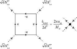
Figure 6: The microscopic process which contributes the boson-boson repulsive force in the BEC region. The thin line expresses propagation of fermion, while the external dashed line represents incoming/outgoing boson. $\sqrt{\mathstrut d}$ is the wavefunction renormalization. The arrow indicated on the line represents the flow of baryon charge.

Now we discuss the fluctuation transport property in the BEC regime. In the BEC regime where $\mu<m$ is realized, $d$ in turn becomes pure real as shown in Eq. (96). Again by ignoring $d_{2}$ term looking at the dynamics of sufficiently low energy excitation, and by rescaling the field as $\Psi(t,\mbox{\boldmath$x$})=\sqrt{\mathstrut d}\Delta(t,\mbox{\boldmath$x$})$, we arrive at

$$\left[-i\partial_{t}+\frac{a_{T}}{d}-\frac{c\nabla_{\mathstrut\mbox{\scriptsize{\boldmath$x$}}\mathstrut}^{2}}{4md}+\frac{b_{0}}{d^{2}}\sum_{\xi}|\Psi_{\xi}(t,\mbox{\boldmath$x$})|^{2}\right]\Psi_{\eta}(t,\mbox{\boldmath$x$})=0.$$ (110)

It is obvious that this is the Gross-Pitaevskii (GP) equation Pitaevskii ; Gross1 ; Gross2 which describes the low energy excitation above the Bose-Einstein condensate after identifying

$$\mu_{b}\equiv\displaystyle-\frac{a_{T}}{d},\quad M_{b}\equiv\displaystyle 2m\,\frac{d}{c},\quad\frac{4\pi a_{sb}}{M_{b}}=\displaystyle\frac{b_{0}}{d^{2}},$$ (111)

where $\mu_{b}$, $M_{b}$, and $a_{sb}$ are the effective chemical potential, the effective boson mass, and the effective scattering length for $s$-wave boson-boson scattering. In Fig. 6, we show the schematic Feynman graph which contributes to $a_{sb}$. When the temperature goes below $T_{c}$, $\mu_{b}$ becomes positive indicating the instability to formation of the Bose-Einstain condensate.

We see that the fluctuation becomes propagating in the BEC regime as in the nonrelativistic fermion system melo93 . This is because a gap $(2m-2\mu)$ appears between the continuum excitation and $\omega=0$ due to the formation of bound state. Therefore, the low energy fluctuation about the equilibrium cannot decay in this region; the fluctuation with wavenumber $k$ can decay only via the nonlinear term, i.e., the scattering among soft modes.

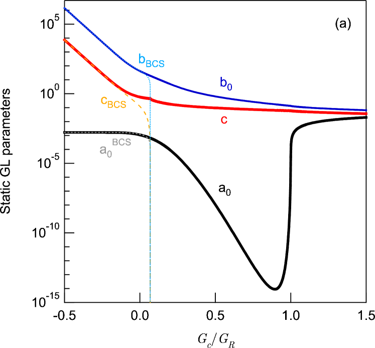
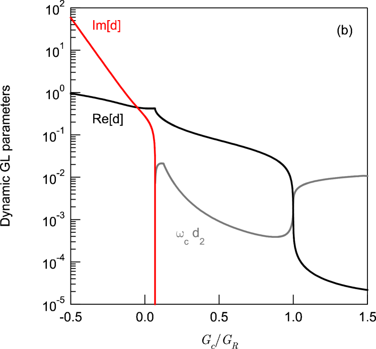
Figure 7: (a)  The static GL parameters as a function of $G_{R}^{-1}$. $a_{0}$, $c$, and $b$ are the mass-squared parameter, the diffusion constant, and the interaction parameter. $a_{0}^{\rm BCS}$, $c^{\rm BCS}$, and $b^{\rm BCS}$ are the weak coupling analytic approximations $(\mu_{c}\gg T_{c})$ of $a_{0}$, $c$, and $b$. (b)  The dynamic GL parameters. $d$ ($d_{2}$) is the coefficient for the first (second) time-derivative of the TDGL equation. $\omega_{c}\equiv{\rm min.}(T_{c},|\mu_{c}-m|)$ is the limit energy such that the low energy GL expansion is valid for $\omega\ll\omega_{c}$.

We now study the situation $|d\omega|\ll d_{2}\omega^{2}$; we will see that, in the RBEC phase, there actually exists such an “intermediate” frequency regime $d/d_{2}\mathrel{\mathchoice{\vbox{\offinterlineskip\halign{\hfil$\displaystyle#$\hfil\cr<\crcr\vskip 0.0pt\cr\sim\crcr}}}{\vbox{\offinterlineskip\halign{\hfil$\textstyle#$\hfil\cr<\crcr\vskip 0.0pt\cr\sim\crcr}}}{\vbox{\offinterlineskip\halign{\hfil$\scriptstyle#$\hfil\cr<\crcr\vskip 0.0pt\cr\sim\crcr}}}{\vbox{\offinterlineskip\halign{\hfil$\scriptscriptstyle#$\hfil\cr<\crcr\vskip 0.0pt\cr\sim\crcr}}}}|\omega|$ where the expansion is still valid $(\omega\ll\omega_{c}\equiv{\rm min.}\,(T_{c},|\mu-m|))$. In such regime, we find $d_{2}$ becomes pure real and positive. By rescaling field $\Psi(t,\mbox{\boldmath$x$})=\sqrt{\mathstrut d_{2}}\Delta(t,\mbox{\boldmath$x$})$, we obtain the relativistic Gross-Pitaevskii (RGP) equation (or simply the Klein-Gordon equation with $\Phi^{4}$ interaction) Fukuyama:2005jq :

$$\left[\partial_{t}^{2}-v_{s}^{2}\nabla_{\mathstrut\mbox{\scriptsize{\boldmath$x$}}\mathstrut}^{2}+M^{2}+\lambda\sum_{\xi}|\Psi_{\xi}(t,\mbox{\boldmath$x$})|^{2}\right]\Psi_{\eta}(t,\mbox{\boldmath$x$})=0,$$ (112)

where $v_{s}$, $M^{2}$ are the velocity and the effective mass of soft mode. $\lambda$ represents the two body repulsive force between soft modes. They are

$$v_{s}^{2}\equiv\frac{c}{4md_{2}},\quad M^{2}\equiv\frac{a_{T}}{d_{2}},\quad\lambda\equiv\frac{b_{0}}{d_{2}^{2}}.$$ (113)

When the temperature goes below $T_{c}$, $M^{2}$ becomes negative. The soft mode then becomes tachyonic without nonlinear terms, which signals the instability to the formation of nonzero Bose-Einstein condensate $\langle\Psi(0,\mbox{\boldmath$0$})\rangle\neq 0$.

To see which region of $(\omega,k)$-space is governed by the RGP (or GP) equation, we look at the dispersion relation of the fluctuation in the (R)BEC region. The dispersion is given by the solution of

$$-d\omega-d_{2}\omega^{2}+\frac{ck^{2}}{4m}+a_{T}=0,$$ (114)

At the critical temperature $(a_{T}=0)$, we find

$$\omega_{k}=\frac{d}{2d_{2}}\left(\sqrt{\mathstrut 1+\frac{cd_{2}}{md^{2}}k^{2}}-1\right).$$ (115)

For a sufficiently small wavenumber $k\ll\sqrt{\mathstrut\frac{md^{2}}{cd_{2}}}$,

$$\omega_{k}\sim\frac{k^{2}}{2M_{b}},$$ (116)

where $M_{b}$ is defined in Eq. (111). This is the dispersion of nonrelativistic particle with velocity $v=k/M_{b}$. In the opposite case, the dispersion is approximated as

$$\omega_{k}\sim v_{s}k,$$ (117)

with $v_{s}$ defined by Eq. (113). This is the dispersion of phonon with velocity $v_{s}$. We note that as $d_{2}$ becomes large such that $d_{2}\gg d^{2}m/c$, the momentum region where the dynamics of fluctuation is described by the RGP equation becomes wide. This is the case when we increase the attraction between quarks as we will see later.

In FIG. 7(a) and (b) show the numerical results for the static and dynamic GL parameters from the weak coupling BCS regime to the ultra-strong coupling RBEC regime. The weak coupling approximation for these parameters are also indicated by several thin dashed lines. One can see the drastic change going from the BCS to the RBEC particularly in the dynamic GL parameters. From these results, we shall discuss the character change of the soft mode, and transport properties.

IV.1 How does the static property of the soft mode evolve with the crossover?

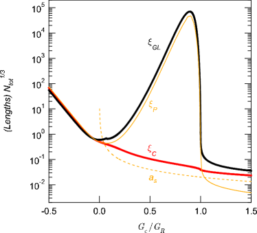
Figure 8: The GL coherence length $\xi_{\rm GL}$ and the Cooper pair size $\xi_{c}$ evaluated on $(\mu_{c}(G_{R}),T_{c}(G_{R}))$. The Pippard length is shown by the line indicated by $\xi_{p}$. $a_{s}$ is the scattering length for $s$-wave quark-quark scattering. These are plotted in the unit of the mean inter-fermion distance $N_{\rm tot}^{-1/3}$.

We first focus on the GL coherence length Eq. (92). As noted, the static disturbance to the system restores at this healing length. Also the anomalous heat capacity $\delta C_{\rm a}$ per unit volume is controlled by this length as

$$\frac{\delta C_{\rm a}}{V}=\frac{N_{c}(N_{c}-1)}{2}\frac{1}{8\pi\xi_{\rm GL}^{3}}t_{r}^{-1/2}.$$ (118)

Furthermore, this quantity is known to appear in the intensity of the diverging conductivity at $T=T_{c}$ Aslamazov ; Maki ; Larkin .

$$\sigma_{\rm AL}\sim\frac{g^{2}}{\xi_{\rm GL}}t_{r}^{-1/2}.$$ (119)

where $g$ is the gauge coupling.

In FIG. 8, we show the GL coherence length $\xi_{\rm GL}$ as a function of $G_{R}^{-1}$. The Cooper pair size $\xi_{c}(T_{c})$ and the Pippard length $\xi_{p}$ are also shown. In the weak coupling region, all these scales exhibit almost the same behaviour. In particular, the weak coupling “universal relation” $\xi_{\rm GL}/\xi_{p}=0.74$ (see Eq. (93)) is satisfied in good accuracy. However, once one goes into the BEC region, these scales start to deviate. First, the pair size $\xi_{c}$ becomes smaller than the mean inter-fermion distance, which supports the picture of independent bosons. In this regime, the pair size $\xi_{c}$ is approximated by the scattering length $a_{s}$ rather than $\xi_{p}$ as noted before. In contrast, the GL coherence length $\xi_{\rm GL}$ takes a minimum between the BCS and BEC regimes as nonrelativistic calculation melo97 . On the other hand, the behaviour of $\xi_{\rm GL}$ is approximated by the Pippard length $\xi_{p}\sim v_{F}/\Delta_{0}$ which is defined in the weak coupling regime though. This fact suggests that, the gap parameter not only has the role of the order parameter but also plays a physical role to determine the response to the static disturbance.

Ginzburg-Levanyuk region: The above derived low energy effective theories may fail in describing the dynamics of soft modes when $T$ is very close to $T_{c}$, i.e., they cannot be applied in the critical region. In this critical region the thermodynamic quantities diverge with the anomalous power law. We can estimate this region by Ginzburg-Levanyuk criterion ref:Leva59 ; ref:Ginz60 . We first define the order parameter averaged in the sphere $V_{T}=4\pi(\xi_{\rm GL}/\sqrt{\mathstrut t_{r}})^{3}$, a characteristic size of static fluctuation:

$$\Psi_{\eta}=\frac{1}{V_{T}}\int_{V_{T}}d\mbox{\boldmath$x$}\Delta_{\eta}(\mbox{\boldmath$x$}).$$ (120)

Then we estimate the magnitude of the thermal average of fluctuation in the gaussian approximation.

$$\begin{array}[]{rcl}\langle{\Psi}_{\eta}^{*}\Psi_{\xi}\rangle_{\rm th}&=&\frac{\delta_{\eta\xi}}{V_{T}}\int_{V_{T}}d\mbox{\boldmath$x$}\langle\Delta^{*}_{1}(\mbox{\boldmath$x$})\Delta_{1}(\mbox{\boldmath$0$})\rangle_{\rm th}\\[8.61108pt] &=&\delta_{\eta\xi}\frac{mT}{c}\frac{1-1/e}{\pi\xi_{\rm GL}}\sqrt{\mathstrut t_{r}}.\end{array}$$ (121)

If $a_{T}\langle\Psi^{*}_{\eta}\Psi_{\eta}\rangle_{\rm th}$ becomes smaller than the quartic term $\frac{b}{2}|\Psi_{\eta}|^{2}|\Psi_{\xi}|^{2}$, then the mean field approximation fails due to higher terms in the soft mode action; this condition is

$$t_{r}=\frac{T-T_{c}}{T_{c}}\mathrel{\mathchoice{\vbox{\offinterlineskip\halign{\hfil$\displaystyle#$\hfil\cr<\crcr\vskip 0.0pt\cr\sim\crcr}}}{\vbox{\offinterlineskip\halign{\hfil$\textstyle#$\hfil\cr<\crcr\vskip 0.0pt\cr\sim\crcr}}}{\vbox{\offinterlineskip\halign{\hfil$\scriptstyle#$\hfil\cr<\crcr\vskip 0.0pt\cr\sim\crcr}}}{\vbox{\offinterlineskip\halign{\hfil$\scriptscriptstyle#$\hfil\cr<\crcr\vskip 0.0pt\cr\sim\crcr}}}}\frac{N_{c}(N_{c}-1)}{2}\frac{b_{0}T_{c}(1-1/e)}{8a_{0}^{2}\xi_{\rm GL}^{3}}.$$ (122)

When the temperature is in the above range, the Ginzburg-Landau approximation fails to describe the anomalous divergence of the thermodynamic quantities like the heat capacity Kitazawa:2005vr . We must note that the critical region estimated by above formula is not small in the RBEC regime, which means we need to go beyond the quartic approximation in order to describe the soft mode there in the quantitative level.

IV.2 What about the dynamic nature of fluctuation?

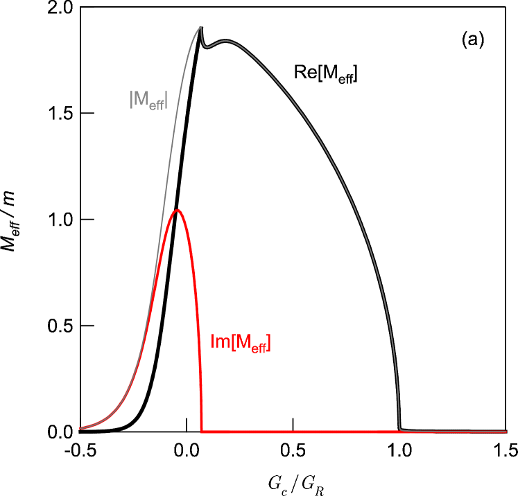
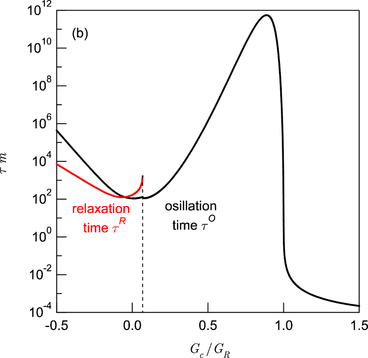
Figure 9: (a)  The complex effective mass as a function of $G_{R}$, which determines the time dependence of the fluctuation with finite $k$ at $T\cong T_{c}$. (b)  The oscillation time $\tau^{O}$ and the relaxation time $\tau^{R}$ for the fluctuation in the long wavelength limit.

We now look at the dynamic property. We first ignore the effect of $d_{2}$ looking at the low frequency regime. Then the complex pole ($\omega_{\rm pole}$) of the dynamic susceptibility in the TDGL approximation should be given by

$$\begin{array}[]{rcl}\omega_{\rm pole}&=&\displaystyle\frac{ck^{2}}{4md}+\frac{a_{T}}{d}=\displaystyle\frac{k^{2}}{2M_{\rm eff}}-i\frac{1}{\tau^{O}t_{r}^{-1}}+\frac{1}{\tau^{R}t_{r}^{-1}}.\end{array}$$ (123)

where the effective (complex) mass $M_{\rm eff}$, the relaxation time $\tau^{R}$, and the oscillation time $\tau^{O}$ are defined by

$$\begin{array}[]{rcl}M_{\rm eff}&=&\displaystyle 2m\frac{d}{c},\quad\tau^{R}=\frac{|d|^{2}}{a_{0}\,{\rm Im}\,d},\quad\tau^{O}=\frac{|d|^{2}}{a_{0}\,{\rm Re}\,d}.\\[8.61108pt] \end{array}$$ (124)

In the BEC region, $M_{\rm eff}$ is real and coincides with effective boson mass $M_{b}$ defined in Eq. (111). For the stability that the fluctuation about the thermal equilibrium is not tachyonic, ${\rm Im}\,\omega_{\rm pole}<0$ should be satisfied. This requires both $T\mathrel{\mathchoice{\vbox{\offinterlineskip\halign{\hfil$\displaystyle#$\hfil\cr>\crcr\vskip 0.0pt\cr\sim\crcr}}}{\vbox{\offinterlineskip\halign{\hfil$\textstyle#$\hfil\cr>\crcr\vskip 0.0pt\cr\sim\crcr}}}{\vbox{\offinterlineskip\halign{\hfil$\scriptstyle#$\hfil\cr>\crcr\vskip 0.0pt\cr\sim\crcr}}}{\vbox{\offinterlineskip\halign{\hfil$\scriptscriptstyle#$\hfil\cr>\crcr\vskip 0.0pt\cr\sim\crcr}}}}T_{c}$ and ${\rm Im}\,d\mathrel{\mathchoice{\vbox{\offinterlineskip\halign{\hfil$\displaystyle#$\hfil\cr>\crcr\vskip 0.0pt\cr\sim\crcr}}}{\vbox{\offinterlineskip\halign{\hfil$\textstyle#$\hfil\cr>\crcr\vskip 0.0pt\cr\sim\crcr}}}{\vbox{\offinterlineskip\halign{\hfil$\scriptstyle#$\hfil\cr>\crcr\vskip 0.0pt\cr\sim\crcr}}}{\vbox{\offinterlineskip\halign{\hfil$\scriptscriptstyle#$\hfil\cr>\crcr\vskip 0.0pt\cr\sim\crcr}}}}0$, and our numerical result shows that the latter is actually satisfied (see FIG. 7(b)).

The fluctuation with a wavenumber $k$ behaves as

$$\Delta_{\eta}(t,k)\sim\exp\left(-i\frac{tk^{2}}{2M_{\rm eff}}-i\frac{t}{\tau^{R}t_{r}^{-1}}+\frac{t}{\tau^{O}t_{r}^{-1}}\right).$$ (125)

For $T\cong T_{c}$, the fluctuation looks like $\Delta_{\xi}(t,k)|_{T=T_{c}}=e^{-t/\tau^{D}_{k}}\sin(t/\tau^{P}_{k}+{\rm const.})$ where $\tau_{k}^{D}=\frac{2|M_{\rm eff}|}{k^{2}}\frac{1}{{\rm Im}\,M_{\rm eff}}$ and $\tau_{k}^{P}=\frac{2|M_{\rm eff}|}{k^{2}}\frac{1}{{\rm Re}\,M_{\rm eff}}$ are the diffusion and propagating times. Thus the complex effective mass determines whether the fluctuation with a finite momentum $k$ is diffusive or propagating. In contrast, $\tau^{R}$ and $\tau^{O}$ determine how the long wavelength limit of the fluctuation behaves for $T\mathrel{\mathchoice{\vbox{\offinterlineskip\halign{\hfil$\displaystyle#$\hfil\cr>\crcr\vskip 0.0pt\cr\sim\crcr}}}{\vbox{\offinterlineskip\halign{\hfil$\textstyle#$\hfil\cr>\crcr\vskip 0.0pt\cr\sim\crcr}}}{\vbox{\offinterlineskip\halign{\hfil$\scriptstyle#$\hfil\cr>\crcr\vskip 0.0pt\cr\sim\crcr}}}{\vbox{\offinterlineskip\halign{\hfil$\scriptscriptstyle#$\hfil\cr>\crcr\vskip 0.0pt\cr\sim\crcr}}}}T_{c}$. In this case, the fluctuation looks like as $\Delta_{\eta}(t,0)\sim e^{-t/\tau^{R}t_{r}^{-1}}\sin(t/\tau^{O}t_{r}^{-1}+{\rm const.})$ where $\tau^{R}$ and $\tau^{O}$ are the relaxation and oscillation times.

FIG. 9(a) shows the complex effective mass $M_{\rm eff}$ as a function of $G_{R}$, and (b) shows the relaxation time $\tau^{R}(G_{R})$ and the oscillation time $\tau^{O}(G_{R})$. We can see from figure (a) that the fluctuation is diffusive ($\tau^{P}_{k}\gg\tau^{D}_{k}$) in the BCS regime, while in the BEC regime, the pair fluctuation is of propagating ($\tau^{P}_{k}\ll\tau^{D}_{k}$) because of the reality of boson melo93 . In contrast to the nonrelativistic calculation melo93 ; Haussmann , $|M_{\rm eff}|\neq 2m$ in the strong coupling limit. It decreases due to the binding effect as the coupling becomes stronger. Also the long wavelength limit of the pair excitation is of overdamped in the BCS side ($\tau^{R}\ll\tau^{O}$) while it is oscillating mode in the BEC side ($\tau^{R}=\infty$) because of ${\rm Im}\,d=0$. This is again attributed to the bound state gap.

IV.3 Relativistic Gross-Pitaevskii equation

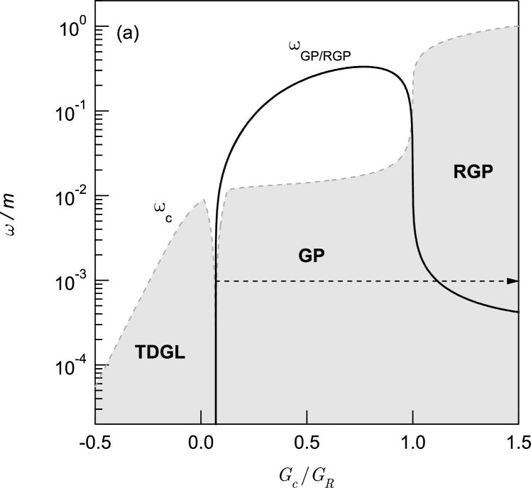
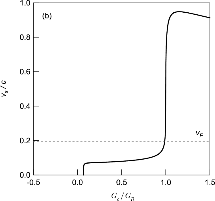
Figure 10: (a) The three regions where the fluctuation is described by TDGL, GP, and RGP equations. The low energy expansion is allowed for the shaded area where $\omega<\omega_{c}\equiv{\rm min.}(T_{c},|\mu_{c}-m|)$. (b) The group velocity of the fluctuation (boson), $d\omega_{k}/dk$, evaluated along the light dashed arrow in (a).

We have shown that there may exist the three distinct-$(\omega,k)$ regions where the fluctuation is described by the TDGL, GP, and RGP equations. FIG. 10(a) shows where in the $\omega$-region these three equations govern the dynamics of soft mode. The shaded area satisfies the condition $\omega<\omega_{c}\equiv{\rm min.}(T_{c},|\mu_{c}-m|)$ where the low energy expansion is valid. As in the nonrelativistic case melo93 , the validity breaks down in the very vicinity of the BCS-BEC crossover due to $|\mu_{c}-m|\to 0$. The solid line indicated by $\omega_{\rm GP/RGP}$ divides the $\omega$-space into two pieces, one in which the GP equation applies, and the other where the RGP equation applies. We determined this boundary by

$$\omega_{\rm GP/RGP}=\frac{(\sqrt{\mathstrut 2}-1)d}{2d_{2}},$$ (126)

which is evaluated by equating $\frac{cd_{2}}{md^{2}}k^{2}$ in Eq. (115) to unity; if $\omega\gg\omega_{\rm GP/RGP}$ the dispersion of the fluctuation is approximated by Eq. (117), and in the opposite case with $\omega\ll\omega_{\rm GP/RGP}$, it is approximated by the nonrelativistic dispersion, Eq. (116). We see that the $\omega$-region where the RGP equation describes the fluctuation rapidly grows when the system goes into the RBEC region. This is obviously because boson is light in the RBEC region.

FIG. 10(b) shows the group velocity of the fluctuation mode, i.e., $v_{s}=\frac{d\omega_{k}}{dk}$ (with $\omega_{k}$ defined by Eq. (115)) evaluated along the dashed arrow in figure (a). The velocity of fluctuation is smaller than the Fermi velocity $v_{F}$ and is almost independent of $G_{R}$ in the BEC region. It rapidly grows at $G_{c}/G_{R}\sim 1$ where the system goes into the RBEC phase; the speed $v_{s}$ becomes comparable to the speed of light; this is also consistent with the fact that the boson is light in this regime.

IV.4 Interaction between soft modes

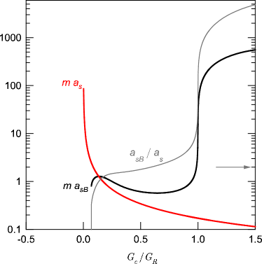
Figure 11: The fermion-fermion scattering length $a_{s}=mG_{R}/4\pi$, and the boson-boson scattering length $a_{sb}$. The arrow indicates $2$, the strong coupling limit which the ratio $a_{sb}/a_{s}$ approaches in the nonrelativistic calculation melo93 .

As we have discussed, there are multi-body interaction among soft modes. To the lowest order beyond the gaussian approximation, we found the repulsive two-body interaction which causes a binary collision. From Eq. (111), the scattering length for this collision is given by

$$a_{sb}=\frac{mb_{0}}{2\pi cd},$$ (127)

which determines the scattering cross section in the soft limit $(s\to 4M_{b}^{2})$ in the C.M. frame as

$$\sigma_{b}=4\pi a_{sb}^{2}=\frac{m^{2}b_{0}^{2}}{\pi c^{2}d^{2}}.$$ (128)

In Fig. 11, we show the fermion-fermion scattering length $ma_{s}$ and the boson-boson scattering length $ma_{sb}$ as a function of $G_{R}^{-1}$. Also its ratio $a_{sb}/a_{s}$ is depicted. When $G_{R}^{-1}$ is increased beyond the BCS/BEC boundary, the boson scattering length first decreases, i.e., the weaker boson-boson repulsion in the stronger fermion-fermion attraction melo93 . This is because the boson-boson interaction is microscopically induced only via the dissociation of boson in the intermediate state as shown in Fig. 6; it becomes harder to dissociate the boson in the stronger coupling. When $G_{R}^{-1}$ is further increased and the RBEC is approached, the boson-boson scattering length rapidly increases, and the nonrelativistic limit value of $a_{sb}/a_{s}$, $2$ melo93 , is significantly exceeded . This is because the temperature is large ($T_{c}>2\mu_{c}$) in the RBEC regime, which favors dissociation.

IV.5 Smooth change of transport properties

We here discuss some of the transport properties on the basis of the dynamic equations obtained in the previous section. In the nonrelativistic superconductor, it is known that the fluctuating pair fields affect the electric conductivity above $T_{c}$ Aslamazov ; Maki ; Larkin . In the context of two-flavor color superconductivity, it is noted in Kitazawa:2001ft that these soft modes may affect not only transport coefficients but also the dilepton spectrum.

We here focus on the shear viscosity near the critical temperature and derive approximate formulas for the viscosities in three regions. To do this, we employ the semi-classical Kubo’s formula and also the Boltzmann equation for soft modes in the sprit that the short range quantum effects are already integrated out in the low-energy coefficients in the soft mode action. For this to be correct, soft modes should be only dilutely distributed in the phase space such that they can be described by the classical effective theory. Technically, this means that we only take the “thermal average” of the soft mode distribution in the Kubo’s formula. We will make a short statement regarding the validity of this treatment in the end of this section.

Shear viscosity due to the soft mode diffusion in the BCS regime: We now look at the precursory soft mode contribution to the shear viscosity, $\eta_{s}$, in the BCS regime. In the rotationally symmetric system considering here, the shear viscosity is formally given by the quantum Kubo’s formula Hosoya:1983id ,

$$\eta=\lim_{\omega\to 0}\frac{1}{\omega}\int d\mbox{\boldmath$x$}\int_{0}^{\infty}dte^{i(\omega+i\delta)t}\langle[\hat{T}_{xy}(\mbox{\boldmath$x$},t),\hat{T}_{xy}(\mbox{\boldmath$0$},0)]\rangle,$$ (129)

where $\hat{T}_{ij}$ denotes the traceless part of the energy-momentum tensor. First thing we have to do is to derive the classical approximation ($\omega\ll T$) of the Kubo’s formula Eq. (129). From the spectral representation of the real part of Eq. (129), we find for $\omega\ll T$,

$$\begin{array}[]{rcl}{\rm Re}\,\eta&\cong&\displaystyle\beta\int d\mbox{\boldmath$x$}\int_{0}^{\infty}dt\,\langle\hat{T}_{xy}(t,\mbox{\boldmath$x$})\hat{T}_{xy}(0,\mbox{\boldmath$0$})\rangle.\end{array}$$ (130)

Note that we have no longer the commutation in the bracket. We now replace $\hat{T}_{xy}$ by the classical stress tensor and the expectation by the thermal average looking only at the contribution from soft modes (with $\omega\ll T$) to the viscosity $\eta_{s}$. For this purpose, we first extract the soft mode contribution to the stress-momentum tensor which we denote by $\delta T_{ij}$. The stress arising from soft modes is

$$\begin{array}[]{rcl}\delta T_{ij}(t,x)&=&-\delta_{ij}f_{\rm eff}(\Delta,\Delta^{*})\\[8.61108pt] &&+\frac{c}{4m}\left[\partial_{i}\Delta_{\eta}^{*}(t,x)\partial_{j}\Delta_{\eta}(t,x)+(i\leftrightarrow j)\right]\end{array}$$ (131)

This is followed by calculation of the free energy shift $\delta F_{\rm eff}=-\int d\mbox{\boldmath$x$}\delta T_{ij}\frac{\partial}{\partial x_{j}}u_{i}(x)$ under the small distortion $x_{i}\to x_{i}^{\prime}=x_{i}+u_{i}(\mbox{\boldmath$x$})$. The shear viscosity from fluctuating pair fields is then given by

$$\begin{array}[]{rcl}\eta_{s}&=&{\displaystyle\beta}\displaystyle\lim_{\mathstrut\mbox{\scriptsize{\boldmath$p$}}\mathstrut\to\mathstrut\mbox{\scriptsize{\boldmath$0$}}\mathstrut}\int_{0}^{\infty}dt\frac{1}{Z_{\rm eff}}\int{\mathcal{D}}\Delta{\mathcal{D}}\Delta^{*}\,e^{-\beta F_{\rm eff}(\Delta,\Delta^{*})}\delta T_{xy}(t,\mbox{\boldmath$p$})\delta T_{xy}(0,-\mbox{\boldmath$p$})\\[8.61108pt] &=&\displaystyle{\beta}\left(\frac{c}{4m}\right)^{2}\lim_{\mathstrut\mbox{\scriptsize{\boldmath$p$}}\mathstrut\to\mathstrut\mbox{\scriptsize{\boldmath$0$}}\mathstrut}\int\frac{d\mbox{\boldmath$\mbox{\boldmath$q$}$}}{(2\pi)^{3}}(2q_{x}q_{y}+q_{x}p_{y}+q_{y}p_{x})^{2}\int_{0}^{\infty}dt\langle\Delta^{\eta}_{\mathstrut\mbox{\scriptsize{\boldmath$q$}}\mathstrut+\mathstrut\mbox{\scriptsize{\boldmath$p$}}\mathstrut,t}\Delta^{\xi*}_{\mathstrut\mbox{\scriptsize{\boldmath$q$}}\mathstrut+\mathstrut\mbox{\scriptsize{\boldmath$p$}}\mathstrut,0}\rangle_{\rm th}\langle\Delta^{\eta*}_{\mathstrut\mbox{\scriptsize{\boldmath$q$}}\mathstrut,t}\Delta^{\xi}_{\mathstrut\mbox{\scriptsize{\boldmath$q$}}\mathstrut,0}\rangle_{\rm th}.\\[8.61108pt] \end{array}$$ (132)

Here $\langle\cdots\rangle_{\rm th}$ denotes the thermal average at $t=0$, i.e., $\frac{1}{Z_{\rm eff}}\int{\mathcal{D}}\Delta{\mathcal{D}}\Delta^{*}(\cdots)$. The diagrammatic interpretation for the above formula is given in Fig. 12. To proceed further, we use the standard ansatz that the time evolution of the fluctuation is determined by the classical TDGL equation in the gaussian approximation;

$$\Delta_{\mathstrut\mbox{\scriptsize{\boldmath$q$}}\mathstrut,t}=U_{\mathstrut\mbox{\scriptsize{\boldmath$q$}}\mathstrut,t}\Delta_{\mathstrut\mbox{\scriptsize{\boldmath$q$}}\mathstrut,0}=e^{-i\frac{ct}{4md}(\mathstrut\mbox{\scriptsize{\boldmath$q$}}\mathstrut^{2}+\xi_{\rm GL}^{-2}t_{r})}\Delta_{\mathstrut\mbox{\scriptsize{\boldmath$q$}}\mathstrut,0}.$$ (133)

The gaussian approximation to $F_{\rm eff}[\Delta,\Delta^{*}]$ is also essential in order for the replacement of the expectation of $\Delta^{4}$ by the product of the two body Green’s functions in Eq. (132) to be valid. By taking the identity $\langle\Delta_{\mathstrut\mbox{\scriptsize{\boldmath$q$}}\mathstrut,0}^{\xi}\Delta_{\mathstrut\mbox{\scriptsize{\boldmath$q$}}\mathstrut,0}^{\eta*}\rangle_{\rm th}=\frac{4mT}{c}\frac{\delta_{\eta\xi}}{\mathstrut\mbox{\scriptsize{\boldmath$q$}}\mathstrut^{2}+\xi_{\rm GL}^{-2}t_{r}}$ into account, we obtain

$$\begin{array}[]{rcl}\eta_{s}&=&\displaystyle N_{c}(N_{c}-1){T}\frac{4m\,|d|^{2}}{c\,{\rm Im}\,[d]}\int^{q_{c}}\!\!\frac{d\mbox{\boldmath$\mbox{\boldmath$q$}$}}{(2\pi)^{3}}\frac{q_{x}^{2}q_{y}^{2}}{(\mbox{\boldmath$q$}^{2}+\xi_{\rm GL}^{-2}t_{r})^{3}}\\[8.61108pt] &\to&\displaystyle\frac{N_{c}(N_{c}-1)}{30\pi^{2}}\frac{T_{c}\tau^{R}}{\xi_{\rm GL}^{2}/k_{F}},\quad\mbox{(as $T\to T_{c},\,q_{c}=k_{F}$)}.\end{array}$$ (134)

where we have introduced the UV cutoff $q_{c}$ and set $q_{c}=k_{F}$. Unlike the conductivity which diverges as $T\to T_{c}$ like $\frac{g^{2}}{\xi_{\rm GL}\sqrt{\mathstrut t_{r}}}$ Aslamazov ; Maki , the shear viscosity is regular. Also the shear viscosity is proportional to the soft mode relaxation time; the transport coefficients are always proportional to the relaxation time (mean free time) of the quasi-particle according to the relaxation time approximation to the Boltzmann equation. Because of the divergence of the relaxation time $\tau^{R}\to\infty$ at the BCS-BEC crossover point $\mu=m$, this formula fails to describe the shear viscosity in the BEC regime. We thus try the other approach to derive the shear viscosity in the BEC region.

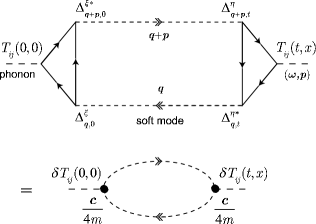
Figure 12: The microscopic process which contributes to the shear viscosity in the BCS region ($\mu_{c}>m$). The same graph expresses the Aslamazov-Larkin type correction to the conductivity if the vertex $T_{ij}(t,\mbox{\boldmath$x$})$ is replaced by the paramagnetic current Kitazawa:2005vr . In our TDGL approach, a phonon couples to two soft modes by the TDGL coefficient ($c/4m$).

Shear viscosity via boson binary collision in the BEC regime: In the BEC regime, the soft fluctuation about the equilibrium cannot decay via the quantum diffusion because of the bound state gap. In reality, however, the soft mode with momentum $k$ decays via the nonlinear term in the GP equation, i.e., the binary collision of soft modes. Here, we simply apply the result from the classical Boltzmann equation for dilute gas of a particle with a hard sphere $r=\sqrt{\mathstrut 2}a_{sb}$. Reichl ; Chapman ; BLTZ ,

$$\begin{array}[]{rcl}\eta_{s}&=&\frac{5\pi}{32\sqrt{\mathstrut 2}}n_{\rm soft}\langle M_{\rm eff}v\rangle_{\rm th}l_{\rm mfp}\\[8.61108pt] &\sim&0.35\times n_{\rm soft}\langle M_{\rm eff}v\rangle_{\rm th}l_{\rm mfp}.\\[4.30554pt] \end{array}$$ (135)

$n_{\rm soft}$ is the soft mode density, and $l_{\rm mfp}$ is the mean free path. $\langle M_{\rm eff}v\rangle_{\rm th}$ is the average momentum of thermally excited soft modes. These are given by

$$\begin{array}[]{rcl}l_{\rm mfp}&=&\displaystyle\frac{1}{n_{\rm soft}\sigma_{sb}}=\frac{\pi c^{2}d^{2}}{n_{\rm soft}m^{2}b_{0}^{2}},\\[12.91663pt] \langle M_{\rm eff}v\rangle_{\rm th}&=&\displaystyle\lambda_{T}^{-1}=\sqrt{\mathstrut\frac{M_{\rm eff}T}{2\pi}}=\sqrt{\mathstrut\frac{mdT}{c\pi}}.\\[4.30554pt] \end{array}$$ (136)

Combining the above results, we arrive at the formula

$$\eta_{s}=\frac{5\sqrt{\mathstrut 2}}{256}\frac{1}{\lambda_{T}a_{sb}^{2}}=\frac{5\pi^{3/2}}{32\sqrt{\mathstrut 2}}\frac{c^{3/2}d^{5/2}\sqrt{\mathstrut T}}{m^{3/2}b_{0}^{2}}.$$ (137)

This equation relates the low energy coefficients in the GP equation to the shear viscosity. We note that this formula is valid only for the classical (dilute) limit, i.e., $n_{\rm soft}a_{sb}^{3},n_{\rm soft}\lambda_{T}^{3}\ll 1$, where $\lambda_{T}=\sqrt{\mathstrut\frac{2\pi}{M_{\rm eff}T}}$ is the thermal de-Broglie length, the quantum radius at $T$.

Shear viscosity via binary collision between light bosons in the RBEC phase: The nonrelativistic formula we have derived above fails in the RBEC regime because of the lightness of boson. The qualitative behaviour of the shear viscosity is Jeon:1994if ; Jeon:1995zm

$$\begin{array}[]{rcl}\eta_{s}&\sim&l_{\rm mfp}\bar{v}\langle\varepsilon+P\rangle_{\rm th}\sim l_{\rm mfp}\bar{v}T\langle s\rangle_{\rm th},\end{array}$$ (138)

where $s$ denotes the entropy density, and $\bar{v}$ is the average velocity of soft modes. In the above formula, we ignored the chemical potential dependent part of the pressure, i.e., $P=\mu n+Ts-\varepsilon\to Ts-\varepsilon$ with $\varepsilon$ being the energy density. The relativistic thermal de-Broglie length is given by Yan

$$\lambda_{RT}=\frac{\pi^{2/3}}{T},$$ (139)

and therefore, the soft mode dynamics is described by the RGP equation we derived in the previous section. $\bar{v}$ and the scattering cross section for a collision between soft modes is estimated as

$$\bar{v}=\sqrt{\mathstrut\frac{c}{4md_{2}}},\quad\sigma_{sb}(s\sim T^{2})\sim\frac{\lambda^{2}}{T^{2}}\sim\frac{b_{0}^{2}}{T^{2}d_{2}^{4}},$$ (140)

with $\lambda$ being the $\Delta^{4}$ coupling (see Eq. (113)). We obtain

$$\eta_{s}\sim\frac{\bar{v}}{\sigma_{sb}}\frac{Ts}{n_{\rm soft}},$$ (141)

where we adopted the simplified notation $s=\langle s\rangle_{\rm th}$ for the equilibrium entropy density. $n_{\rm soft}$ again denotes the density of thermal soft modes. We further simplify the equation by estimating $s/n_{\rm soft}$ in the present gaussian approximation for the soft mode action. The thermodynamic potential coming from soft modes is

$$\begin{array}[]{rcl}\delta\Omega&=&\frac{N_{c}(N_{c}-1)}{4}T\sum_{N}\int\frac{d\mathstrut\mbox{\scriptsize{\boldmath$P$}}\mathstrut}{(2\pi)^{3}}\sum_{\sigma=\pm}\log\left(-d_{2}(i\Omega_{N}+\sigma\mu)^{2}+\frac{cP^{2}}{4m}+a_{T}\right)\equiv\delta\Omega_{+}+\delta\Omega_{-},\\[8.61108pt] \end{array}$$ (142)

where $\delta\Omega_{\pm}$ represents the bosonic (antibosonic) contribution to the partition function:

$$\begin{array}[]{rcl}\delta\Omega_{\pm}=\frac{N_{c}(N_{c}-1)}{4}T\sum_{N}\int\frac{d\mathstrut\mbox{\scriptsize{\boldmath$P$}}\mathstrut}{(2\pi)^{3}}\log\Big{(}d_{2}\Omega_{N}^{2}+\Big{(}\sqrt{\mathstrut\frac{cP^{2}}{4m}+a_{T}}+\sigma\sqrt{\mathstrut d_{2}}\mu\Big{)}^{2}\Big{)}.\end{array}$$ (143)

By differentiating the difference $(\delta\Omega_{+}-\delta\Omega_{-})$ with respect to $\mu$, we find the following formula for the soft mode density in the limit $T\to T_{c}$ and $T_{c}\gg\mu$,

$$\begin{array}[]{rcl}n_{\rm soft}&=&\left(\frac{d_{2}m}{c}\right)^{3/2}\frac{16\zeta(3)}{\pi^{2}}\frac{N_{c}(N_{c}-1)}{2}T_{c}^{3}.\end{array}$$ (144)

Also, we take the same limit in Eq. (142) to find the Stephan-Boltzmann pressure

$$\begin{array}[]{rcl}\delta\Omega=\frac{N_{c}(N_{c}-1)}{2}\frac{\pi^{2}}{45}\left(\frac{4m}{c}\right)^{3/2}d_{2}^{2}T_{c}^{4}.\end{array}$$ (145)

Then by differentiating this with respect to $T_{c}$, we find

$$\begin{array}[]{rcl}s&=&\langle s\rangle_{\rm th}=\frac{N_{c}(N_{c}-1)}{2}\frac{4\pi^{2}}{45}\left(\frac{4m}{c}\right)^{3/2}d_{2}^{2}T_{c}^{3}.\end{array}$$ (146)

Combining all the above, we obtain the following parametric dependence of the shear viscosity

$$\eta_{s}\sim\sqrt{\mathstrut d_{2}}\bar{v}\frac{T_{c}}{\sigma_{sb}}.$$ (147)

Then, adjusting the prefactor to the result of the relativistic Boltzmann equation BLTZ , we end up with

$$\eta_{s}=\frac{3}{10\pi}\sqrt{\mathstrut\frac{c}{4m}}\frac{T_{c}}{\sigma_{sb}}\sim\frac{3}{20\pi}\frac{c^{1/2}d_{2}^{4}}{m^{1/2}b_{0}^{2}}T_{c}^{3}.$$ (148)

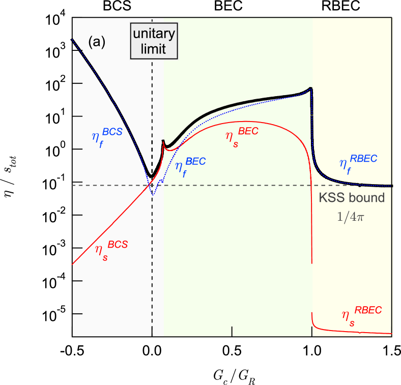
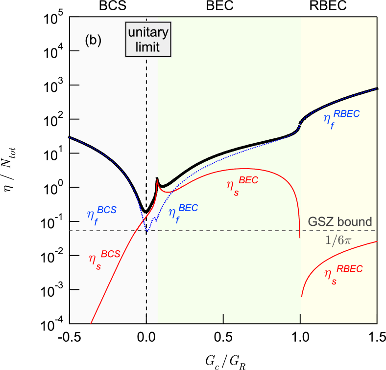
Figure 13: (a) The shear viscosity to entropy ratios from soft modes, $\eta_{s}^{\rm BCS}$, $\eta_{s}^{\rm BEC}$, and $\eta_{s}^{\rm RBEC}$ as a function of four-fermion coupling $G_{R}^{-1}$ (thin solid lines). The dashed lines indicated by $\eta_{f}^{\rm BCS}$ $\eta_{f}^{\rm BEC}$, and $\eta_{f}^{\rm RBEC}$ correspond to the shear viscosities from fermions in BCS/BEC and RBEC regimes. The total viscosity, the sum of the fermion- and boson- originated viscosities, are shown by bold solid line. The “KSS bound”, ${1}/{4\pi}$, is shown by the horizontal dashed line. At the unitary limit, the cross section for the low energy $s$-wave fermion scattering diverges as $\sim 1/k^{2}$ with $k$ being the relative momentum. (b) The shear viscosity to quark number ratios. The dashed line indicated by “GSZ bound” is the minimum bound, $1/6\pi$, proposed in Gelman:2004fj .

Summarizing our results, shear viscosities arising from soft modes in the three regimes are

$$\begin{array}[]{rcl}\eta_{s}({\rm BCS})&=&\displaystyle\frac{4}{5\pi^{2}}\frac{m|d|^{2}k_{F}T_{c}}{c{\rm Im}\,d},\\[12.91663pt] \eta_{s}({\rm BEC})&=&\displaystyle\frac{5\pi^{3/2}}{32\sqrt{\mathstrut 2}}\frac{c^{3/2}d^{5/2}\sqrt{\mathstrut T_{c}}}{m^{3/2}b_{0}^{2}},\\[12.91663pt] \eta_{s}({\rm RBEC})&=&\displaystyle\frac{3}{20\pi}\frac{c^{1/2}d_{2}^{4}}{m^{1/2}b_{0}^{2}}T_{c}^{3}.\\[8.61108pt] \end{array}$$ (149)

The system has fermion’s degrees of freedom as well as soft modes. As for the viscosity from fermion-fermion binary collision, we estimate that in the nonrelativistic region by $\eta_{f}=\frac{5\pi\bar{k}}{32\sqrt{\mathstrut 2}}\frac{1+\bar{k}^{2}a_{s}^{2}}{4\pi a_{s}^{2}}$ with $\bar{k}$ being the average momentum of fermions, and that in the RBEC regime by $\eta_{f}=\frac{3}{40\pi^{2}}\frac{T_{c}^{3}}{m^{2}a_{s}^{2}}$. We also evaluate $\bar{k}$ simply by $\bar{k}=\sqrt{\mathstrut{\rm max.}\left(\mu^{2}-m^{2},\frac{mT_{c}}{2\pi}\right)}$, i.e., we take the larger of (a) the matter momentum due to the Pauli-blocking, and (b) the thermal momentum.

In FIG. 13, we have examined the above-derived formulas for shear viscosities in three regimes. FIG. 13(a) shows the shear viscosity to entropy density ratio as a function of $G_{R}^{-1}$. This quantity is related to the sound attenuation length by $\Gamma_{s}=\frac{\frac{4}{3}\eta+\zeta}{s_{\rm tot}T}$ with $\zeta$ being the bulk viscosity. For a hard sphere particle gas, $\zeta\ll\eta$ both for nonrelativistic $T\ll m$ and relativistic $T\gg m$ situations Reichl ; Chapman ; BLTZ . For the fluid-dynamic picture to be valid, this length must be much smaller than the time scale of the fluid-dynamic evolution of system. From the figure, we can see that in the weak coupling BCS regime, the total viscosity is dominated by contribution from the fermion binary scattering, and that from the soft mode diffusion is negligible . As the coupling $G_{R}^{-1}$ becomes larger, $\eta_{f}^{\rm BCS}$ monotonically decreases with the behaviour $\sim a_{s}^{2}\sim 1/|G_{R}|^{2}$; because the cross section for the fermion binary scattering monotonically increases and this effect on the shear viscosity overcomes the effect of the decrease in the average momentum $\bar{k}$. In contrast, $\eta_{s}^{\rm BCS}$ monotonically increases because the relaxation time of the soft mode, $\tau_{R}T_{c}$, becomes large. As the unitary limit $G_{R}^{-1}=0^{-}\,(a_{s}=-\infty)$ is approached, $\eta_{f}^{\rm BCS}$ rapidly decreases and crosses the “KSS bound” ($1/4\pi$), the minimum bound of $\eta/s$ conjectured out by Kovtun, Son and Starinets Kovtun:2004de . However owing to the viscosity due to soft modes, the sum of the viscosity ratios, $\eta_{s}+\eta_{f}$, does not lower the bound.

When the crossover point $G_{c}/G_{R}\sim 0.068$ where $\mu_{c}=m$ is closely approached, $\eta_{s}^{\rm BCS}$ rapidly diverges due to the divergent relaxation time ($\tau_{R}=\infty$) at $\mu_{c}=m$. As noted, however, this is not physical for the following two reasons: (i) The soft mode with $k$ actually relaxes via the non-linear interaction caused in the TDGL action. (ii) The low energy expansion fails in the vicinity of $\mu_{c}=m$ because of the absence of expansion scales. In short, the singularity in the crossover point is attributed both to our gaussian approximation to the soft mode relaxation, and to the breakdown of the low energy expansion melo93 .

In summary, we found the following facts. (1) Soft mode may play important role to the shear viscosity near the unitary regime. In fact, the model calculation performed here shows that it makes the minimum bound for shear viscosity proposed in Kovtun:2004de remain valid. On the other hand, it is completely dominated by fermionic processes in the weak coupling BCS regime. (2) Shear viscosity takes almost minimum near the unitary limit in the present model calculation. It is close to the minimum bounds Kovtun:2004de ; Gelman:2004fj . It is also noteworthy that the bulk viscosity vanishes in the unitary limit Son:2005tj . These suggest that the intermediate of the BCS/BEC crossover is rather liquid-like as conjectured in Gelman:2004fj .

Finally we must note that our ansatz that the short range quantum correlation is completely incorporated in the coefficients in the low energy soft mode action may not be good approximation in the BEC and RBEC regimes. In fact, the ratio of the thermal de-Broglie length of soft mode to the average distance between soft modes is not smaller than the unity, taking around $2\sim 4$. Further theoretical investigations are indeed needed in future to clarify how secondary quantum corrections affect the shear viscosity.

V The density dependence and the quantum fluctuation

We here again look at some static aspects of crossover. In Sec. V.1, we ask how the characteristics of the critical temperature as a function of $G_{R}^{-1}$ depends on quark number density which we have fixed so far. We then discuss whether quark matter with the standard choice of diquark coupling exhibits the crossover. In Sec. V.2, we look at how large the effect of quantum fluctuation in the “boson sea”, which we have neglected so far.

V.1 The density dependence; what about the ultra-relativistic limit of the crossover?

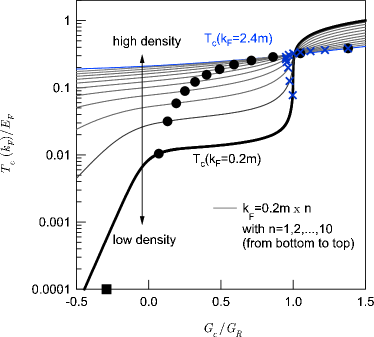
Figure 14: The $k_{F}$-dependence of the critical temperature as a function of $G_{c}/G_{R}$. From bottom to top, the Fermi momentum increases as $k_{F}=0.2m,0.4m,\cdots,2.4m$. The large point located on each critical line represents the BCS/BEC crossover point where $\mu_{c}=m$ holds, while the large cross corresponds to the BEC/RBEC boundary which we estimated by $T_{c}=2\mu_{c}$. The large square put on the horizontal axis indicates the standard choice of the diquark attraction, i.e., $\frac{G}{4}\sim\frac{3}{4}G_{s}$ with $G_{s}=2.17/\Lambda^{2}$ set to reproduce the dynamical quark mass $M_{q}=400\,{\rm MeV}$ in vacuum.

So far we have worked with a fixed Fermi momentum $k_{F}=0.2m$. We now study how the BCS/BEC/RBEC crossover will be affected by the change of quark density. In FIG. 14, we show the $k_{F}$-dependence of $T_{c}$ as a function of the four-Fermi coupling, $G_{R}^{-1}$. As the system becomes denser, the critical temperature increases monotonically . At the same time, the BCS/BEC crossover boundary ($\mu_{c}=m$) indicated by the large point shifts to a larger coupling. As noted before, this is because the Pauli-blocking prevents the formation of bound boson in medium. In addition, the characteristic change in the shape of ($T_{c}$, $G_{R}^{-1}$)-relation gets somewhat smeared and seems to vanish for $k_{F}\mathrel{\mathchoice{\vbox{\offinterlineskip\halign{\hfil$\displaystyle#$\hfil\cr>\crcr\vskip 0.0pt\cr\sim\crcr}}}{\vbox{\offinterlineskip\halign{\hfil$\textstyle#$\hfil\cr>\crcr\vskip 0.0pt\cr\sim\crcr}}}{\vbox{\offinterlineskip\halign{\hfil$\scriptstyle#$\hfil\cr>\crcr\vskip 0.0pt\cr\sim\crcr}}}{\vbox{\offinterlineskip\halign{\hfil$\scriptscriptstyle#$\hfil\cr>\crcr\vskip 0.0pt\cr\sim\crcr}}}}m$. Moreover, a typical diquark coupling strength, $\frac{3}{4}$ of the scaler coupling $G_{s}\Lambda^{2}=2.17$ chosen so that the dynamical quark mass $400\,{\rm MeV}$ is reproduced at vacuum, is located below the unitary coupling $G_{R}^{-1}=0$ (see the large square on the horizontal axis). From these points, we conclude that quark matter only with light flavors hardly exhibits the BCS-BEC crossover. We need a somewhat exotic situation where (i) the in-medium constituent quark mass is comparable to $\mu$ and (ii) the $(qq)$ attraction between constituent quarks is stronger than that in the $(q\bar{q})$ channel in order for the BCS-BEC crossover to be realized in possible quark matter inside compact stars.

V.2 How does the quantum fluctuation affect the crossover?

We here examine how large the quantum fluctuation we have ignored so far can be. As we discussed in Sec. II.2, the gaussian fluctuation consists of two parts, i.e., the Nozières–Schmit-Rink correction

$$\begin{array}[]{rcl}\Omega_{\rm NSR}(\mu,T)&=&-\frac{N_{c}(N_{c}-1)}{2}\int_{-\infty}^{\infty}\!\frac{d\omega}{\pi}\frac{d\mathstrut\mbox{\scriptsize{\boldmath$P$}}\mathstrut}{(2\pi)^{3}}\\[8.61108pt] &&\times\tilde{f}_{B}(\omega)\delta^{\rm Ren}_{\mu,T}(\omega,\mbox{\boldmath$P$}),\\[8.61108pt] \end{array}$$ (150)

and the “quantum fluctuation” which remains finite as $T\to 0$ in the presence of finite $\mu$

$$\begin{array}[]{rcl}\Omega_{\rm qfl}(\mu,T)&=&-\frac{N_{c}(N_{c}-1)}{2}\int_{-\infty}^{\infty}\!\frac{d\omega}{\pi}\frac{d\mathstrut\mbox{\scriptsize{\boldmath$P$}}\mathstrut}{(2\pi)^{3}}\\[8.61108pt] &&\times\frac{\epsilon(\omega)}{2}\left[\delta^{\rm Ren}_{\mu,T}(\omega,\mbox{\boldmath$P$})-\delta^{\rm Ren}_{0}(\omega,\mbox{\boldmath$P$})\right].\end{array}$$ (151)

$\omega$-integral in $\Omega_{\rm qfl}$ is finitem, while the remaining momentum integral is quadratically divergent and thus we need to introduce a new three momentum cutoff $\Lambda_{B}$. In principle, there exists no a priori relation between the fermionic cutoff $\Lambda$ and the bosonic cutoff $\Lambda_{B}$. But it is reasonable that $\Lambda_{B}<\Lambda$ because the short range quantum effects are already taken in part to the bosonic effective lagrangian. Here we shall try two choices, $\Lambda_{B}=0.2\Lambda$ and $\Lambda_{B}=0.3\Lambda$.

Before going into discussion of numerical results, let us little closely look at the structure of quantum fluctuation to see its physical meaning. In order to grab an intuition into this term, we try to estimate the quantum fluctuation by the bound state approximation for the in-medium phase shift; that is

$$\begin{array}[]{rcl}\delta_{\mu,T}(\omega,\mbox{\boldmath$P$})&=&\pi\theta(\omega>E_{B\mathstrut\mbox{\scriptsize{\boldmath$P$}}\mathstrut}^{\mu,T}-2\mu),\\[8.61108pt] &&-\pi\theta(\omega<-E_{\bar{B}\mathstrut\mbox{\scriptsize{\boldmath$P$}}\mathstrut}^{\mu,T}-2\mu),\\[4.30554pt] \end{array}$$ (152)

where $E^{\mu,T}_{B\mathstrut\mbox{\scriptsize{\boldmath$P$}}\mathstrut}$ and $E^{\mu,T}_{\bar{B}\mathstrut\mbox{\scriptsize{\boldmath$P$}}\mathstrut}$ are the boson and antiboson energy dispersions. Then substituting this into Eq. (151) yields

$$\begin{array}[]{rcl}\Omega_{\rm qfl}(\mu,T)&=&\frac{N_{c}(N_{c}-1)}{2}\int^{\Lambda_{B}}\!\!\!\frac{d\mathstrut\mbox{\scriptsize{\boldmath$P$}}\mathstrut}{(2\pi)^{3}}\bigg{[}\frac{E_{{B}\mathstrut\mbox{\scriptsize{\boldmath$P$}}\mathstrut}^{\mu,T}+E_{\bar{B}\mathstrut\mbox{\scriptsize{\boldmath$P$}}\mathstrut}^{\mu,T}}{2}-E_{B\mathstrut\mbox{\scriptsize{\boldmath$p$}}\mathstrut}^{0}\bigg{]},\\[8.61108pt] \end{array}$$ (153)

where the three momentum cutoff $\Lambda_{B}$ is introduced. Now it is clear that this correction is due to the vacuum fluctuation (quantum Casimir pressure for boson). It differs from fermionic one by minus sign. For example, the chiral condensation energy at $T=0$ can be written by the integral of the zero-point energy shift as

$$\begin{array}[]{rcl}\Omega_{\chi\rm SB}&=&-2N_{c}N_{f}\int^{\Lambda}\frac{d\mathstrut\mbox{\scriptsize{\boldmath$p$}}\mathstrut}{(2\pi)^{3}}\bigg{[}{E_{M\mathstrut\mbox{\scriptsize{\boldmath$p$}}\mathstrut}-E_{0\mathstrut\mbox{\scriptsize{\boldmath$p$}}\mathstrut}}\bigg{]}.\\[8.61108pt] \end{array}$$ (154)

We conclude that the quantum fluctuation is interpreted as the “vacuum” energy coming from the in-medium shift of the boson (antiboson) dispersion. In the BCS regime, the above argument will be slightly modified because there is no stable boson in the spectrum. However, even in the BCS regime, it can be understood in the same way; it is the vacuum fluctuation coming from the in-medium spectral shift.

Differentiating Eq. (153) with respect to $\mu$ results in the following expression for the number density from the quantum fluctuation.

$$\begin{array}[]{rcl}N_{\rm qfl}&=&-\frac{N_{c}(N_{c}-1)}{2}\frac{1}{2}\int^{\Lambda_{B}}\!\!\!\frac{d\mathstrut\mbox{\scriptsize{\boldmath$P$}}\mathstrut}{(2\pi)^{3}}\biggl{[}\frac{\partial E^{\mu,T}_{B\mathstrut\mbox{\scriptsize{\boldmath$P$}}\mathstrut}}{\partial\mu}+\frac{\partial E^{\mu,T}_{\bar{B}\mathstrut\mbox{\scriptsize{\boldmath$P$}}\mathstrut}}{\partial\mu}\biggr{]}.\\[8.61108pt] \end{array}$$ (155)

Let us recall here that in the bound state approximation, the number density coming from the ordinary thermal fluctuation is given by Eq. (66) where we see that the “effective charge” of (anti)boson deviates from $(\pm)2$. From these points, we can see that a small fraction ${\partial E_{B(\bar{B})\mathstrut\mbox{\scriptsize{\boldmath$P$}}\mathstrut}^{\mu,T}}/{\partial\mu}$ of quark number charge in the thermal fluctuation escapes to the vacuum sector. In the nonrelativistic situation where $m\gg(|\mu-m|,T_{c})$, we can ignore the antiboson contribution to fluctuations. In addition, the effective charge shift is of order $(P^{2}/M_{B}^{2})(\partial M_{B}/\partial\mu)$, which is negligible by definition of nonrelativity, i.e., $(P^{2}/2M_{B}\ll M_{B})$. This argument justifies the ordinary nonrelativistic treatment. Also at high temperature $T\mathrel{\mathchoice{\vbox{\offinterlineskip\halign{\hfil$\displaystyle#$\hfil\cr>\crcr\vskip 0.0pt\cr\sim\crcr}}}{\vbox{\offinterlineskip\halign{\hfil$\textstyle#$\hfil\cr>\crcr\vskip 0.0pt\cr\sim\crcr}}}{\vbox{\offinterlineskip\halign{\hfil$\scriptstyle#$\hfil\cr>\crcr\vskip 0.0pt\cr\sim\crcr}}}{\vbox{\offinterlineskip\halign{\hfil$\scriptscriptstyle#$\hfil\cr>\crcr\vskip 0.0pt\cr\sim\crcr}}}}N_{\rm tot}^{1/3}/M_{B}$, the thermal fluctuation dominates over the quantum fluctuation because of the Bose-enhancement in $N_{\rm NSR}$, i.e., $f_{B}(\omega)\sim T/\omega$ for $\omega\ll T$, and we can safely ignore the quantum fluctuation. Thus, we expect that the effect of the quantum fluctuation becomes less significant with going from the weak coupling BCS regime to the RBEC regime.

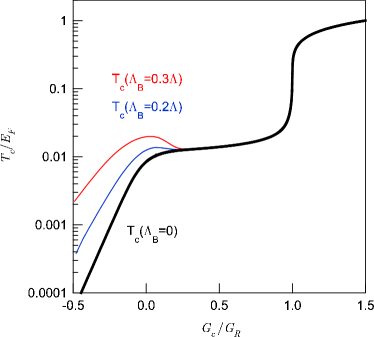
Figure 15: The critical temperature versus the four-Fermi coupling. The bold curve shows the result without the quantum fluctuation, while two thin lines are the results when the quantum fluctuation is incorporated with two choices for cutoff, i.e., $\Lambda_{B}=0.2\Lambda$ (down) and $\Lambda_{B}=0.3\Lambda$ (up).

In FIG. 15, we show how the $(T_{c},G_{R}^{-1})$-relation is affected by the incorporation of the quantum fluctuation. We solved the number equation

$$\begin{array}[]{rcl}\displaystyle N_{c}N_{F}\frac{k_{F}^{3}}{3\pi^{2}}&=&\displaystyle N_{\rm MF}(\mu,T)+N_{\rm NSR}(\mu,T)-\frac{\partial\Omega_{\rm qfl}}{\partial\mu},\\[4.30554pt] \end{array}$$ (156)

together with the Thouless condition Eq. (55) in $(\mu,T)$ to obtain the critical line $(\mu_{c}(G_{R}),T_{c}(G_{R}))$. The bold line is the result without the quantum fluctuation, while two thin lines show the results with two different choices for a cutoff $\Lambda_{B}$ in $\Omega_{\rm qfl}$; the lower (upper) line corresponds to $\Lambda_{B}=0.2\Lambda$ ($0.3\Lambda$). We conclude that the quantum fluctuation greatly affects the critical temperature in the BCS regime. This is a feature which is specific in the relativistic BCS state where the condition $m\gg(|\mu-m|,T_{c})$ does not hold. As anticipated, the effect of quantum fluctuation becomes smaller for the (R)BEC regime where the critical temperature is relatively high ($T_{c}\mathrel{\mathchoice{\vbox{\offinterlineskip\halign{\hfil$\displaystyle#$\hfil\cr>\crcr\vskip 0.0pt\cr\sim\crcr}}}{\vbox{\offinterlineskip\halign{\hfil$\textstyle#$\hfil\cr>\crcr\vskip 0.0pt\cr\sim\crcr}}}{\vbox{\offinterlineskip\halign{\hfil$\scriptstyle#$\hfil\cr>\crcr\vskip 0.0pt\cr\sim\crcr}}}{\vbox{\offinterlineskip\halign{\hfil$\scriptscriptstyle#$\hfil\cr>\crcr\vskip 0.0pt\cr\sim\crcr}}}}N_{\rm tot}^{1/3}/M_{B}$).

Let us finally explain why the quantum fluctuation increases the critical temperature in the BCS regime. The quark number from the vacuum fluctuation is negative as seen in Eq. (155). Then, to keep the quark number unchanged, the quark number from the mean field contribution $N_{\rm MF}(\mu,T)$ should increase. To realize this on the Thouless line in $(\mu,T)$-plane, the line $(\mu,T_{c}(\mu))$ along which the Thouless criterion is satisfied, the temperature should also increase because $T_{c}(\mu)$ is an increasing function as well as $N_{\rm MF}(\mu,T_{c}(\mu))$. So we have to go higher $\mu$ (and $T_{c}(\mu)$) in the $(\mu,T)$-plane in order to keep the total quark number unchanged.

VI Summary and Outlook

We have made an extensive analysis on the static and dynamic aspects of the BCS/BEC crossover in a relativistic superfluid. We first developed the relativistic formulation of the Nozières–Schimit-Rink framework for a Dirac fermion interacting with a four-Fermi point attraction. By carrying out the regularization of the dynamic pair susceptibility using the low energy expansion of the T-matrix in vacuum, we have performed a systematic extension of the nonrelativistic Nozières–Schimit-Rink (NSR) scheme nozieres to a relativistic fermion system. Although we aimed particularly at a possible crossover in quark matter, our framework is general being not restricted to quark matter, and may be used for other relativistic fermion systems such as a possible neutrino superfluidity Kapusta:2004gi inside compact stars at the early stage of their thermal evolution. We have found that in the relativistic case, there is an additional source of fluctuation which we have called the “quantum fluctuation”, and that our approach is consistent with the traditional Nozières–Schmit-Rink framework when $(m\gg|\mu-m|,T_{c})$ where quantum fluctuation is absent.

We have shown by the numerical calculation that three physically distinct regimes appear successively when the attraction is increased: In the weak coupling regime, the system is in the BCS phase where the critical temperature is exponentially smaller than the Fermi energy. When the coupling is increased beyond the unitary limit $a_{s}=\pm\infty$, the system gradually goes into the ordinary BEC phase where the increase of the critical temperature is little suppressed because of the appearance of bound states in the spectrum; in this regime, the increase in the attraction results mainly in the stabilization of boson. However, the critical temperature still shows a gentle increase due to the mass shift of in-medium bosons, which is highly in contrast to the nonrelativistic case. When the attractive coupling is increased further beyond the critical coupling for the Majorana mass formation in vacuum, the system goes into the relativistic BEC (RBEC) phase kapusta where the thermodynamics is dominated by antibosons, antifermions as well as fermions and bosons. To make physics of these three phases transparent, we discussed how the spectral function, occupation numbers, Cooper pair size, and entropy density behave as a function of attraction.

We have also clarified the physical meaning of “quantum fluctuation” and have shown numerically that it greatly affects the critical temperature in the BCS regime, which is also in contrast to the nonrelativistic BCS phase.

In addition to the study of the static aspects of the crossover, we have also studied the evolution of soft mode dynamics. By carrying out the low-energy and long-wavelength expansion of the dynamic pair susceptibility, we have seen how the effective theory for the dynamics of fluctuating pair field changes throughout the crossover. We saw that, in the weak coupling BCS regime, the dynamics of soft modes is described by the time-dependent Ginzburg-Landau (TDGL) theory. Accordingly, the pair fluctuation is an overdamped mode, which dissociates into two fermions in the Fermi sea Abrahams ; melo93 . When the system goes into the BEC regime crossing the unitary limit, the TDGL theory is taken over by the Gross-Pitaevskii (GP) theory as in the nonrelativistic calculation melo93 . In this regime, the low energy pair fluctuating field becomes a propagating mode which cannot decay into fermions because of the bound state gap. When the coupling is further increased and the system goes into the RBEC phase, the relativistic Gross-Pitaevskii (RGP) theory in turn describes a wide kinematical region. In this region, the velocity of the fluctuation is large and the repulsive force between them is also large.

Based on these low energy effective theories, we discussed how the shear viscosity behaves throughout the BCS/BEC crossover. In the spirit that the short range quantum correlation is already taken into the low-energy coefficients in the effective theories, and also on the basis of the ansatz that soft modes are dilutely distributed in the phase space, we estimated the shear viscosity using the classical Kubo’s formula and the Boltzmann equation. We have found that the viscosity in the BCS regime comes from the diffusion process of soft modes, while it comes from the binary scattering between soft modes in the (R)BEC regime. Our model calculation indicated that the soft mode contribution is important near the unitary limit; the shear viscosity to the entropy density ratio takes the minimum in the unitary regime, but the minimum bound of the viscosity proposed by Kovtun, Son and Starinets Kovtun:2004de is kept owing to soft modes.

Unfortunately, as the density is increased $(k_{F}\mathrel{\mathchoice{\vbox{\offinterlineskip\halign{\hfil$\displaystyle#$\hfil\cr>\crcr\vskip 0.0pt\cr\sim\crcr}}}{\vbox{\offinterlineskip\halign{\hfil$\textstyle#$\hfil\cr>\crcr\vskip 0.0pt\cr\sim\crcr}}}{\vbox{\offinterlineskip\halign{\hfil$\scriptstyle#$\hfil\cr>\crcr\vskip 0.0pt\cr\sim\crcr}}}{\vbox{\offinterlineskip\halign{\hfil$\scriptscriptstyle#$\hfil\cr>\crcr\vskip 0.0pt\cr\sim\crcr}}}}m)$, the Pauli-blocking effect against the formation of in-medium bosons, pushes the BCS/BEC crossover boundary to a larger attraction, and makes the crossover characteristics of the critical temperature somewhat ambiguous. Also a typical diquark coupling which is usually adopted in the literature of color superconductivities Abuki:2004zk ; Ruster:2005jc is located well below the unitary point. Based on these points, we have concluded that the following “exotic” conditions are required to have the diquark BEC Nishida:2005ds ; Nawa:2005sb in quark matter core in compact stars; (i) the attraction between quarks is much larger than expected perturbatively Nakamura:2004ur , and (ii) the in-medium fermion mass is larger than the perturbative hard dense loop calculation braaten92 and must be comparable to chemical potential.

Investigating the transport properties for various candidates of the color superconducting phase of quark matter Manuel:2004iv as well as the normal nuclear matter Itoh79 , or exploring the BCS/BEC crossover with paying respect to more realistic conditions of quark matter remains an important issue. It may also be interesting to extend our framework so as to take into account the feedback of soft modes to the fermion propagation in medium, and to ask how the fermion is modified near the critical temperature Kitazawa:2005pp . The self-consistent T-matrix theory Haussmann or the relativistic version of the Brueckner-Hartree-Fock theory BHF will be one of the best ways to study the in-medium fermion property affected by soft modes.

Appendix A Imaginary part of the dynamic pair susceptibility

The imaginary part of the dynamic pair susceptibility can be calculated as

$$\begin{array}[]{lll}&&{\rm Im}\,\chi_{\mu,T}(\omega+i\delta,\mbox{\boldmath$P$})\\[8.61108pt] &&\quad=\theta\big{[}z>\sqrt{\mathstrut 4m^{2}+P^{2}}\big{]}f_{qq}^{\mu,T}(z,P)\\[8.61108pt] &&\quad\quad-\theta\big{[}|z|\leq P\big{]}f_{\rm LD}^{\mu,T}(z,P)\\[8.61108pt] &&\quad\quad-\theta\big{[}z<-\sqrt{\mathstrut 4m^{2}+P^{2}}\big{]}f_{\bar{q}\bar{q}}^{\mu,T}(z,P),\end{array}$$ (157)

where we have defined a variable $z=\omega+2\mu$. We can show the identity $f_{\bar{q}\bar{q}}^{\mu,T}(z,P)=f_{qq}^{-\mu,T}(-z,P)$. The explicit forms for $f_{qq}^{\mu,T}$ and $f_{\bar{q}\bar{q}}^{\mu,T}$ can be found as

$$\begin{array}[]{rcl}f_{qq}^{\mu,T}(z,P)&=&-\frac{\sqrt{\mathstrut z^{2}-P^{2}}}{4\pi}\sqrt{\mathstrut z^{2}-P^{2}-4m^{2}}\\[8.61108pt] &&+\frac{z^{2}-P^{2}}{2\pi P}T\ln\left[\frac{1+e^{\frac{\omega}{2T}+\frac{P}{2T}\sqrt{\mathstrut\frac{z^{2}-P^{2}-4m^{2}}{z^{2}-P^{2}}}}}{1+e^{\frac{\omega}{2T}-\frac{P}{2T}\sqrt{\mathstrut\frac{z^{2}-P^{2}-4m^{2}}{z^{2}-P^{2}}}}}\right],\\[12.91663pt] f_{\rm LD}^{\mu,T}(z,P)&=&\frac{P^{2}-z^{2}}{2\pi P}\omega\\[8.61108pt] &&+\frac{P^{2}-z^{2}}{2\pi P}T\ln\left[\frac{1+e^{-\frac{\omega}{2T}+\frac{P}{2T}\sqrt{\mathstrut\frac{z^{2}-P^{2}-4m^{2}}{z^{2}-P^{2}}}}}{1+e^{\frac{\omega}{2T}+\frac{P}{2T}\sqrt{\mathstrut\frac{z^{2}-P^{2}-4m^{2}}{z^{2}-P^{2}}}}}\right].\\[12.91663pt] \end{array}$$ (158)

$f_{\rm LD}$ is present only for $T\neq 0$, and is called as the Landau damping, i.e., the Cherenkov radiation (absorption) of soft mode from (to) the thermally excited quarks. We can easily check the identity ${\rm Im}\,\chi_{\mu,T}(0,\mbox{\boldmath$P$})=0$ which states that the quasi-quark excitation on the Fermi surface is stable.

References

- (1) F. Karsch and E. Laermann, Phys. Rev. D 50, 6954 (1994).
- (2) F. Karsch and E. Laermann, arXiv:hep-lat/0305025.
- (3) D. J. Gross and F. Wilczek, Phys. Rev. D 8, 3633 (1973); H. D. Politzer, Phys. Rev. Lett. 30, 1346 (1973).
- (4) I. Arsene et al. [BRAHMS Collaboration], Nucl. Phys. A 757, 1 (2005); B. B. Back et al., Nucl. Phys. A 757, 28 (2005); J. Adams et al. [STAR Collaboration], Nucl. Phys. A 757, 102 (2005); K. Adcox et al. [PHENIX Collaboration], Nucl. Phys. A 757, 184 (2005).
- (5) T. Matsui and H. Satz, Phys. Lett. B 178, 416 (1986); E. V. Shuryak, Phys. Lett. B 78, 150 (1978).
- (6) T. Umeda, K. Nomura and H. Matsufuru, Eur. Phys. J. C 39S1, 9 (2005); M. Asakawa and T. Hatsuda, Phys. Rev. Lett. 92, 012001 (2004); S. Datta et al., Phys. Rev. D 69, 094507 (2004).
- (7) D. Molnar and M. Gyulassy, Nucl. Phys. A 697, 495 (2002) [Erratum-ibid. A 703, 893 (2002)].
- (8) D. Teaney, Phys. Rev. C 68, 034913 (2003).
- (9) A. Nakamura and S. Sakai, Phys. Rev. Lett. 94, 072305 (2005).
- (10) P. Arnold, G. D. Moore and L. G. Yaffe, JHEP 0011, 001 (2000); JHEP 0305, 051 (2003).
- (11) P. Kovtun, D. T. Son and A. O. Starinets, Phys. Rev. Lett. 94, 111601 (2005).
- (12) G. Policastro, D. T. Son and A. O. Starinets, Phys. Rev. Lett. 87, 081601 (2001); JHEP 0209, 043 (2002).
- (13) There is still another scenario to interpret the origin of spurious small viscosity; see for example, M. Asakawa, S. A. Bass and B. Muller, Phys. Rev. Lett. 96, 252301 (2006); see also, J. W. Chen and E. Nakano, arXiv:hep-ph/0604138.
- (14) E. V. Shuryak and I. Zahed, Phys. Rev. C 70, 021901 (2004); Phys. Rev. D 70, 054507 (2004).
- (15) Y. A. Simonov, Phys. Lett. B 619, 293 (2005).
- (16) P. Castorina, G. Nardulli and D. Zappala, Phys. Rev. D 72, 076006 (2005).
- (17) L. He, M. Jin and P. Zhuang, arXiv:hep-ph/0511300.
- (18) T. Hatsuda and T. Kunihiro, Phys. Rev. Lett. 55 (1985) 158.
- (19) T. Hatsuda and T. Kunihiro, Phys. Rept. 247, 221 (1994).
- (20) S. P. Klevansky, Rev. Mod. Phys. 64, 649 (1992).
- (21) J. C. Collins and M. J. Perry, Phys. Rev. Lett. 34, 1353 (1975).
- (22) N. Itoh, Prog. Theor. Phys. 44, 291 (1970).
- (23) D. Bailin and A. Love, Phys. Rept. 107, 325 (1984).
- (24) M. Iwasaki and T. Iwado, Phys. Lett. B 350, 163 (1995).
- (25) For reviews, see K. Rajagopal and F. Wilczek, arXiv:hep-ph/0011333; M. G. Alford, Ann. Rev. Nucl. Part. Sci. 51, 131 (2001); G. Nardulli, Riv. Nuovo Cim. 25N3, 1 (2002); S. Reddy, Acta Phys. Polon. B 33, 4101 (2002); T. Sch’́afer, arXiv:hep-ph/0304281; M. Alford, Prog. Theor. Phys. Suppl. 153, 1 (2004).
- (26) M. G. Alford, K. Rajagopal and F. Wilczek, Nucl. Phys. B 537, 443 (1999).
- (27) D. T. Son, Phys. Rev. D 59, 094019 (1999).
- (28) T. Schäfer and F. Wilczek, Phys. Rev. D 60, 114033 (1999).
- (29) W. E. Brown, J. T. Liu and H. c. Ren, Phys. Rev. D 61, 114012 (2000); Phys. Rev. D 62, 054016 (2000).
- (30) T. Schäfer, Nucl. Phys. B 575, 269 (2000).
- (31) M. Alford, C. Kouvaris and K. Rajagopal, Phys. Rev. Lett. 92, 222001 (2004); Phys. Rev. D 71, 054009 (2005).
- (32) K. Fukushima, C. Kouvaris and K. Rajagopal, Phys. Rev. D 71, 034002 (2005).
- (33) H. Abuki, M. Kitazawa and T. Kunihiro, Phys. Lett. B 615, 102 (2005).
- (34) S. B. Ruster, V. Werth, M. Buballa, I. A. Shovkovy and D. H. Rischke, Phys. Rev. D 72, 034004 (2005); D. Blaschke, S. Fredriksson, H. Grigorian, A. M. Oztas and F. Sandin, Phys. Rev. D 72, 065020 (2005); H. Abuki and T. Kunihiro, Nucl. Phys. A 768, 118 (2006).
- (35) M. Ciminale, G. Nardulli, M. Ruggieri and R. Gatto, Phys. Lett. B 636, 317 (2006).
- (36) M. Kitazawa, D. H. Rischke and I. A. Shovkovy, Phys. Lett. B 637, 367 (2006).
- (37) K. Fukushima, Phys. Rev. D 73, 094016 (2006).
- (38) L. He, M. Jin and P. Zhuang, Phys. Rev. D 74, 036005 (2006).
- (39) J. Carlson and S. Reddy, Phys. Rev. Lett. 95, 060401 (2005).
- (40) D. T. Son and M. A. Stephanov, arXiv:cond-mat/0507586.
- (41) E. Gubankova, A. Schmitt and F. Wilczek, Phys. Rev. B 74, 064505 (2006).
- (42) M. Mannarelli, G. Nardulli and M. Ruggieri, arXiv:cond-mat/0604579.
- (43) M. Matsuzaki, Phys. Rev. D 62, 017501 (2000).
- (44) H. Abuki, T. Hatsuda and K. Itakura, Phys. Rev. D 65, 074014 (2002); K. Itakura, Nucl. Phys. A 715, 859 (2003).
- (45) M. Kitazawa, T. Koide, T. Kunihiro and Y. Nemoto, Phys. Rev. D 65, 091504 (2002); Nucl. Phys. A 721, 285 (2003).
- (46) M. Kitazawa, T. Koide, T. Kunihiro and Y. Nemoto, Phys. Rev. D 70, 056003 (2004).
- (47) M. Kitazawa, T. Koide, T. Kunihiro and Y. Nemoto, Prog. Theor. Phys. 114, 117 (2005).
- (48) D.M. Eagles, Phys. Rev. 186, 45 (1969).
- (49) A.J. Leggett, J. Phys. 41, C7 (1980).
- (50) P. Nozières and S. Schmitt-Rink, J. Low. Temp. Phys. 59 195 (1985).
- (51) See, e.g., Q. Chen, J. Stajic, S. Tan, and K. Levin, Phys. Rep. 412, 1 (2005), and references therein.
- (52) H. Stein et al., Z. Phys. A 351, 295 (1995); U. Lombardo, P. Nozières, P. Schuck, H. J. Schulze and A. Sedrakian, Phys. Rev. C 64, 064314 (2001).
- (53) Y. Ohashi and A. Griffin, Phys. Rev. Lett. 89, 130402 (2002); Phys. Rev. A 67, 033603 (2003).
- (54) K. Fukushima, Phys. Rev. D 70, 094014 (2004).
- (55) Y. Nishida and H. Abuki, Phys. Rev. D 72, 096004 (2005);
- (56) L. He and P. Zhuang, arXiv:hep-ph/0703042.
- (57) H.E. Haber and H.A. Weldon, Phys. Rev. Lett. 46, 1497 (1981); J.I. Kapusta, Phys. Rev. D 24, 426 (1981).
- (58) K. Nawa, E. Nakano and H. Yabu, Phys. Rev. D 74, 034017 (2006).
- (59) J. Deng, A. Schmitt and Q. Wang, arXiv:nucl-th/0611097.
- (60) A. H. Rezaeian and H. J. Pirner, Nucl. Phys. A 779, 197 (2006).
- (61) E. Babaev, Int. J. Mod. Phys. A 16, 1175 (2001).
- (62) J. Kinast et. al., Phys. Rev. Lett. 92, 150402 (2004).
- (63) M. Bartenstein et. al., Phys. Rev. Lett. 92, 203201 (2004).
- (64) J. Kinast, A. Tupalov, and J. E. Thomas, Phys. Rev. A 70, 051401(R) (2004) [Erratum: ibid. 71, 029901(E) (2005)].
- (65) J. Kinast, A. Tupalov, and J. E. Thomas, arXiv:cond-mat/0502507.
- (66) K. M. O’Hara et. al., Science 298, 2179 (2002).
- (67) T. Bourdel et. al., Phys. Rev. Lett. 91, 020402 (2003).
- (68) B. A. Gelman, E. V. Shuryak and I. Zahed, arXiv:nucl-th/0410067.
- (69) T. Schäfer, arXiv:cond-mat/0701251.
- (70) D. T. Son, arXiv:cond-mat/0511721.
- (71) C.A. Regal et al., Phys. Rev. Lett. 92, 040403 (2004); M. Bartenstein et al., Phys. Rev. Lett. 92, 120401 (2004); M.W. Zwierlein et al., Phys. Rev. Lett. 92, 120403 (2004).
- (72) There are several theoretical attempts other than the Monte Carlo simulations Montecarlo to deal with the thermodynamics of the unitary Fermi gas beyond the mean field description. The epsilon expansion about the two and four space dimensions is one of them. See, Y. Nishida and D. T. Son, Phys. Rev. Lett. 97, 050403 (2006); arXiv:cond-mat/0607835. The Ward-Luttinger framework with the Baym-Kadanoff approximation is examined in R. Haussmann, W. Rantner, S. Cerrito, and W. Zwerger, arXiv:cond-mat/0608282. expansion is also applied to the unitary gas. See, P. Nikolić, and S. Sachdev, arXiv:cond-mat/0609106.
- (73) J. Carlson, S. -Y. Chang, V. R. Pandharipande, and K. E. Schmidt, Phys. Rev. Lett. 91, 050401 (2003); G. E. Astrakharchik, J. Boronat, J. Casulleras, and S. Giorgini Phys. Rev. Lett. 93, 200404 (2004); A. Bulgac, J. Drut, and P. Magierski, Phys. Rev. Lett. 96, 090404 (2006); D. Lee, Phys. Rev. B 73, 115112 (2006).
- (74) J. I. Kapusta, Phys. Rev. Lett. 93, 251801 (2004).
- (75) A. Tokumitu, K. Miyake and K. Yamada, Phys. Rev. B 47, 11988 (1993).
- (76) C.A.R. Sá de Melo, M. Randeria, and J.R. Engelbrecht, Phys. Rev. Lett 71,3202 (1993).
- (77) R. Haussmann, Z. Phys. B 91, 291 (1993); Phys. Rev. B 49, 12 975 (1994).
- (78) H. Abuki, Prog. Theor. Phys. 110, 937 (2003).
- (79) C.A.R. Sá de Melo, M. Randeria, and J.R. Engelbrecht, Phys. Rev. B 55, 15153 (1997).
- (80) E. Abrahams and T. Tsuneto, Phys. Rev. 152, 416 (1966).
- (81) D. N. Voskresensky, Phys. Rev. C 69, 065209 (2004).
- (82) K. Iida and G. Baym, Phys. Rev. D 63, 074018 (2001) [Erratum-ibid. D 66, 059903 (2002)]; I. Giannakis and H. c. Ren, Phys. Rev. D 65, 054017 (2002),
- (83) For the case of vanishing fermion mass , similar expressions are obtained in M. Kitazawa, Fluctuations of Diquark-pair Field and Precursory Phenomena in Color Superconductivity (Ph. D. thesis, Kyoto University, Jan. 2006); M. Kitazawa, T. Koide, T. Kunihiro, Y.Nemoto, Talk at Quark Matter 2004 (Oakland, CA, Jan. 14, 2004); the converging parts in their results coincide with ours when the massless limit is taken and the contribution from antiquarks is suppressed.
- (84) L.P. Pitaevskii, Zh. Eksp. Teor. fiz. 40, 646 (1961).
- (85) E.P. Gross, Nuovo Cimento 20, 454 (1961).
- (86) E.P. Gross, J. Math. Phys. 4, 195 (1963).
- (87) T. Fukuyama and M. Morikawa, arXiv:astro-ph/0509789.
- (88) L.G. Aslamazov, A.I. Larkin, Soviet Solid State 10, 875 (1968); Phys. Letters 26A, 238 (1968).
- (89) K. Maki, Prog. Theor. Phys. 39, 897 (1968); 40, 193 (1968); R.S. Thompson, Phys. Rev. B1, 327 (1970).
- (90) A.I. Larkin and A.A. Varlamov, arXiv:cond-mat/0109177.
- (91) A. P. Levanyuk, Sov. Phys. JETP 9, 571 (1959).
- (92) V. L. Ginzburg, Sov. Phys. Solid state 2, 1824 (1960).
- (93) D.S. Petrov, C.Salomon, and G.V. Shlyapnikov, Phys. Rev. Lett. 93, 090404 (2004); Phys. Rev. A 71, 012708 (2005).
- (94) Y. Ohashi, J. Phys. Soc. Jpn. 74, 2659 (2005).
- (95) A. Hosoya, M. a. Sakagami and M. Takao, Annals Phys. 154, 229 (1984).
- (96) Reichl, LE, A Modern Course in Statistical Physics (Univ. Texas Press, Austin, 1991).
- (97) S. Chapman and T.G. Cowling, The Mathematical Theory of Non-Uniform Gases (Cambridge University Press, London, 1939).
- (98) C. Cercignani and G. M. Kremer, The Relativistic Boltzmann Equation: Theory and Applications (Birkh’́auser, Basel, 2002).
- (99) S. Jeon, Phys. Rev. D 52, 3591 (1995).
- (100) S. Jeon and L. G. Yaffe, Phys. Rev. D 53, 5799 (1996).
- (101) Zijun Yan, Eur. J. Phys. 21, 625 (2000).
- (102) A. Nakamura and T. Saito, Prog. Theor. Phys. 112, 183 (2004).
- (103) E. Braaten and R.D. Pisarski, Phys. Rev. D 45, R1827 (1992).
- (104) C. Manuel, A. Dobado and F. J. Llanes-Estrada, JHEP 0509, 076 (2005) [arXiv:hep-ph/0406058].
- (105) E. Flowers and N. Itoh, Astrophys. J. 230, 847 (1979).
- (106) M. Kitazawa, T. Kunihiro and Y. Nemoto, Phys. Lett. B 631, 157 (2005).
- (107) P. Ring and P. Schuck, Nuclear Many-Body Problem (Springer, New York, 1980).