Abstract

The rate of monopole decay into a dyon and an electron in an inhomogeneous external electric field is calculated by semiclassical methods. Comparison is made to an earlier result where this quantity was calculated for a constant field. Experimental and cosmological tests are suggested.

1 Spontaneous and Induced Decay in External Fields

Spontaneous non-perturbative processes of particle production in QFT (Schwinger processes), or vacuum decay processes have been studied since the historic papers of Euler–Heisenberg and Schwinger [1, 2] on $e^{+}e^{-}$ generation in a constant electromagnetic field. Voloshin, Kobzarev, Okun [3] were the first to treat false vacuum decay in a scalar field theory with a stable and a metastable vacuum states. Later Callan and Coleman [4, 5] gave this problem a 1-loop treatment, calculating both the exponent and the preexponential factor of false vacuum decay probability.

Consideration of induced [6, 7] non-perturbative particle creation was a natural extension of the scope of the problems described above. The term “induced” denotes the situation in which the initial state is not vacuum, but rather contains some particle(s). False vacuum decay in a scalar and spinor field theory, induced by presence of an external particle acting as a “catalyst” or “nucleation center”, was treated semiclassically up to 1-loop preexponential in [8].

On the other hand, generalization of Schwinger processes description can be thought of as extending the class of fields in which the appropriate process takes place. The original Euler and Heisenberg calculation in QED was performed for a constant field. For harmonic plane waves calculations had first been done by Schwinger in the cited paper. One can make sure [9] that the same expression is true for adiabatically varying fields. Narozhny and Nikishov [10] calculated exactly the effective Lagrangian in an electric field, dependent on time as $E(t)\sim\frac{1}{\cosh^{2}(\Omega t)}$. A semiclassical treatment of a broad class of fields was given in [11]. Semiclassical methods were further developed basing upon WKB approximation [12] and the so called “worldline instanton method” [13, 14, 15]. To mention some other exact results, Fried and Woodard [16] gave an expression for arbitrary light-cone coordinate dependent field $E(x_{0}\pm x_{1})$. For a comprehensive review of recent developments in Euler — Heisenberg effective actions the reader may consult Dunne’s review [17]. This extensive list (most part of which has been left behind in order not to overload the reader) of Schwinger processes in inhomogeneous external fields is mostly related to QED processes. Some authors also dealt Hawking radiation in a Schwinger-like manner [18, 19]. It should be emphasized that most of the papers on inhomogeneous field vacuum decay consider spontaneous processes.

In the present short paper we suggest combining the both generalizations of Schwinger processes. The possibility of an induced monopole decay into a dyon and an electron was first suggested in [20]. Later it was calculated in a constant electric field in [21] up to leading classical exponential factor. This problem deserves attention per se, but below we also give reasons for astrophysicists to be interested in such processes.

The paper is organized as follows. In section 2 we describe the general techniques of dealing particle decay in terms of Euclidean 1-particle path integral. The sub-barrier trajectories and the leading exponential factor are calculated in section 3. The circumstances under which the process considered might become significant for observers, are investigated in section 4. In section 5 we discuss our results.

2 Quasi-Classical Approximation to Path Integral

We are going to study ’t Hooft–Polyakov (non point-like) monopole and dyon. The masses of these particles $M_{m}$ and $M_{d}$ are of order of the scale $\frac{M_{W}}{\alpha}$ where $M_{W}$ is generally the scale at which spontaneous gauge symmetry breaking takes place (the mass of W-boson), $\alpha$ coupling constant. At the same time, their sizes are of the order of magnitude $M_{W}^{-1}$, thus in weak coupling limit de Broglie’s wavelengths of monopole and dyon are far smaller then corresponding sizes, therefore, these particles are essentially classical objects.

On the other hand, ’t Hooft–Polyakov monopole does not possess a well-established local field-theoretical description. That is why it is reasonable to treat monopole and dyon in terms of 1-particle theory (quantum mechanics), evaluating (bosonic) Feynman path integrals semiclassically with restriction on the trajectories of classical motion $r\gg M_{W}^{-1}$, where $r$ is a typical trajectory size. We are going to study monopole propagator in imaginary (Euclidean) time. To do that semiclassically, one should first find closed-loop trajectories in Euclidean time, and then calculate determinants, corresponding to quantum fluctuations around them. It is essential to take into account only closed loops contributions because only paths with finite classical action on them are relevant.

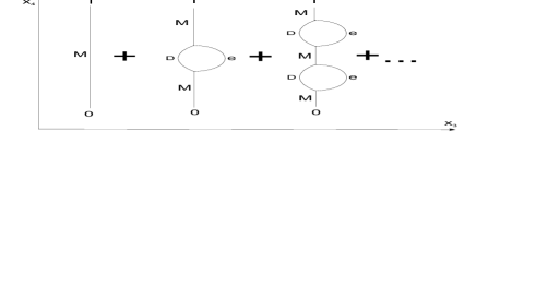
Figure 1: Full 1-loop Green function of a monopole is obtained by summing over all the insertions of electron-dyon loop into monopole’s Euclidean trajectory.

To find the monopole decay probability in an inhomogeneous external field one has to calculate corrections to its propagator in the presence of external electric field. What kind of trajectories will those corrections correspond to at the classical level? As monopole is now not forbidden (due to the presence of the field) to decay into an electron and a dyon, these are configurations containing, beside the monopole pieces, dyon and electron pieces. Therefore, finding the full Green function of a monopole in an external field is equivalent to evaluating Green function with arbitrary number of electron-dyon loop insertions

$$G(T,0)=G^{(0)}(T,0)+G^{(1)}(T,0)+G^{(2)}(T,0)+\cdots$$

The free propagator $G^{(0)}(T,0)$ corresponds to the diagram without dyon-electron loop insertion, $G^{(1)}(T,0)$ denotes Green function with one insertion of electron-dyon loop etc., see Fig. (1). Note that the diagrams of Fig.1 are not Feynman graphs, but are simply the classical trajectories in $Ox_{4}x_{3}$ plane. However, resummation of all electron-dyon loop insertions resembles closely the analogous resummation of all one-particle irreducible vacuum polarization diagram insertions.

Taking into account that the electric charge of the magnetic monopole is zero and using the first quantized approach, the propagator of the monopole in the Euclidean time can be written as follows

$$G^{(0)}(T,0)=\int\mathcal{D}ye^{-M_{m}\int^{T}_{0}\sqrt{\dot{y}^{2}}d\tau}\sim e^{-M_{m}T}\sqrt{\frac{M}{T^{3}}},$$

where $y(t)$ is the monopole variable. The first correction comes from Euclidean-time configuration, shown in Fig. 2.

Figure 2: One-loop Euclidean configuration (“instanton” with winding number $n=1$).

Note that electron and dyon can go round the loop multiply, winding over it with some respective winding numbers $m,n$. This corresponds to the dashed trajectories in Fig. 3. Closed trajectories classified according to their winding number, will be called, following Dunne and Schubert [14], “worldline instantons”. They are analogous to Yang–Mills instanton-antiinstanton pairs.

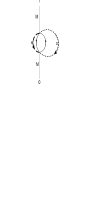
Figure 3: One-loop Euclidean configuration with multiply winding trajectories (“worldline instantons”). Dashed bold arcs correspond to extra winding paths compared to Fig.2, arrows indicate winding direction.

Propagator correction becomes after resummation over winding number $m,n$

$$G^{(1)}_{resummed}(x,z)\sim\sum_{m,n}K_{m,n}e^{-S^{(m,n)}_{cl}}$$ (1)

Here $x=(0,0,0,0),\,z=(T,0,0,0)$ are monopole initial and final Euclidean coordinates. Equivalent notation $G(x,z)=G(T,0)$ will be used for such configurations.

To give the reader the feeling of how $S^{(m,n)}_{cl}$ can be organized, spontaneous vacuum decay case in QED may be brought as an example. Configurations with greater winding number $n$ would give, in general, $S^{(n)}_{cl}\sim nS_{cl}$, i.e. $n$ times greater classical action, and the preexponential factor would depend on $n$ as $K_{n}=\frac{1}{n^{2}}K_{1}$. In the present case, it is reasonable to expect $S^{(m,n)}_{cl}\sim mS^{(e)}_{cl}+nS^{(d)}_{cl}$.

This resummation is not being performed here, only first term $K_{1,1}e^{-S_{cl}^{(1,1)}}$ in the sum being left. Below $K_{1,1}$ will be denoted simply $K$, $S_{1,1}$ as $S_{cl}$. This resummation would be necessary only in case of $S_{cl}\to 0$, otherwise the contribution of higher winding number terms is strongly suppressed. As $S_{cl}\to 0$, both the approximation of point-like monopole and the semiclassical approximation break down, so the interest to this resummation is mostly hypothetical.

For the lowest winding numbers $m=1,\,n=1$, the first correction due to electron-dyon loop is given as

$$G^{(1)}(T,0)=\int\mathcal{D}ye^{-M_{m}\int\sqrt{\dot{y}^{2}}d\tau}\mathcal{D}x\mathcal{D}ze^{-S[x,z,A]},$$ (2)

where action $S[x(u),z(v),A]$ is the common action for the charged particles (dyon and electron) in the external field $A_{\mu}$, $x(t)$ and $z(t)$ are respectively electron and dyon coordinates, their worldlines being parametrized by $u,v$

$$S[x,z,A]=m\int\sqrt{\dot{x}^{2}}du+ie\int A^{ext}(x)\dot{x}du+M_{d}\int\sqrt{\dot{z}^{2}}dv-ie\int A^{ext}(z)\dot{z}dv\,\,.$$

Monopole coordinate is easily integrated out, as monopole does not interact with the electric field,

$$\int\mathcal{D}ye^{-M_{m}\int\sqrt{\dot{y}^{2}}d\tau}\mathcal{D}x\mathcal{D}ze^{-S[x,z,A]}\sim\int e^{-M_{m}(T-h[x,z,A])}\mathcal{D}x\mathcal{D}ze^{-S[x,z,A]},$$ (3)

here $h$ is the vertical size of the loop (see Fig. 2).

The remaining path integral has a more complicated structure of modes. It always has zero modes, corresponding to the shifts of the loop. This will contribute a preexponential factor of $J[x(t),z(t),A]$, which is the Jacobian, arising due to the substitution of variables: normalized zero modes coefficients to the collective coordinates (position of the loop).

The other part of the preexponential factor will come from the non-zero modes. Among them there will be at least one negative mode, corresponding to the overall inflation of electron-dyon loop. Presence of extra negative modes is not evident without a special investigation [21]. In general, the path integral yields

$$G^{(1)}(T,0)=\int d^{4}yG^{(0)}(x,y)G^{(0)}(y+\Delta y,z)Ke^{-S_{cl}}$$ (4)

where $S_{cl}$ is the action of dyon and electron in the external field on a classical path with proper boundary conditions (see Fig.2). The integral over $d^{4}y$ emerges due to integrating over all positions of the loop, and the two free Green’s functions belong to the purely monopole trajectories. Shift $\Delta y$ accounts for non-zero size of the loop, and can be neglected as the condition $T\gg\Delta y$ is imposed.

$K$ contains contributions from the Jacobian and from non-zero modes

$$K=J[x(t),z(t),A]\left(\frac{\mathrm{det}F}{\mathrm{det}F_{0}}\right)^{-\frac{1}{2}}$$

Fluctuation operator $F$ can be found in [21], whereas $F_{0}$ is normalization operator, analogous to operator of fluctuations around trivial vacuum configuration in false vacuum decay problems.

We have just given a sketch of structure of the whole expression for the propagator, as below we are going to be interested mainly in the leading semiclassical exponent, leaving the preexponential part for a more sophisticated analysis in future.

How can  (4) be put into direct correspondence to the mass shift of the particle? If the full Green’s function is $G(x,z)\approx\frac{1}{(2\pi)^{4}}\int\frac{e^{ik(x-z)}}{k^{2}+m^{2}+\delta m^{2}}$, mass shift $\delta m^{2}$ being imaginary or real, then expanding in the powers of $\delta m^{2}$ one gets for the variation of Green’s function

$$\delta G(x,z)=G^{(1)}(x,z)=-\delta m^{2}\int d^{4}yG^{(0)}(x,y)G^{(0)}(y+\Delta y,z)$$

Comparing this with  (4), one makes sure that

$$\delta m^{2}=Ke^{-S_{cl}}$$

3 Exponential factor

We are going to do path integral over electron and dyon coordinates by steepest descent approximation, applying the ideas of world-line instanton method due to Dunne and Schubert [14, 15] to induced decay problem. To find the exponential factor of the probability one should solve classical equations of motion for dyon and electron in an external electromagnetic field, find closed configuration of Euclidean trajectories and minimize the action on them with regard to trajectory parameters. A single-pulse electric field directed along $Ox_{3}$ axis

$$E_{3}=E_{0}\frac{1}{\cosh^{2}(\omega t)}$$

will be considered.

Equations of motion will be of the form

$$m\frac{d}{du}\frac{\dot{x}_{\mu}}{\sqrt{\dot{x}^{2}}}=-ieF_{\mu\nu}(x)\dot{x}_{\nu}$$

$$M_{d}\frac{d}{dv}\frac{\dot{z}_{\mu}}{\sqrt{\dot{z}^{2}}}=ieF_{\mu\nu}(z)\dot{z}_{\nu}$$

where $m,M_{d}$ are electron and dyon masses respectively. Here for convenience, dimensionless parameters $\gamma=\frac{m\omega}{eE}$, $\alpha=\frac{m}{M_{d}}$, $\beta=\frac{M_{m}}{M_{d}}$ are introduced. Solution to these equations for the field $A_{3}(x_{4})=-i\frac{E}{\omega}\tan(\omega x_{4})$ will be for the electron and for the dyon respectively

$$x_{3}(u) = \frac{m}{eE}\frac{1}{\gamma\sqrt{1+\gamma^{2}}}\textrm{arcsinh}\left(\gamma\cos(2\pi u)\right)-a$$

$$x_{4}(u) = \frac{m}{eE}\frac{1}{\gamma}\arcsin\left(\frac{\gamma}{\sqrt{1+\gamma^{2}}}\sin(2\pi u)\right),u\in\left[-u_{0},u_{0}\right]$$

$$z_{3}(v) = -\frac{m}{eE}\frac{1}{\gamma\sqrt{1+\frac{\gamma^{2}}{\alpha^{2}}}}\textrm{arcsinh}\left(\frac{\gamma}{\alpha}\cos(2\pi v)\right)+b$$

$$z_{4}(v) = \frac{m}{eE}\frac{1}{\gamma}\arcsin\left(\frac{\gamma}{\sqrt{\alpha^{2}+\gamma^{2}}}\sin(2\pi v)\right),v\in\left[-v_{0},v_{0}\right],$$

where $a$, $b$, $u_{0}$, $v_{0}$ are some constants.

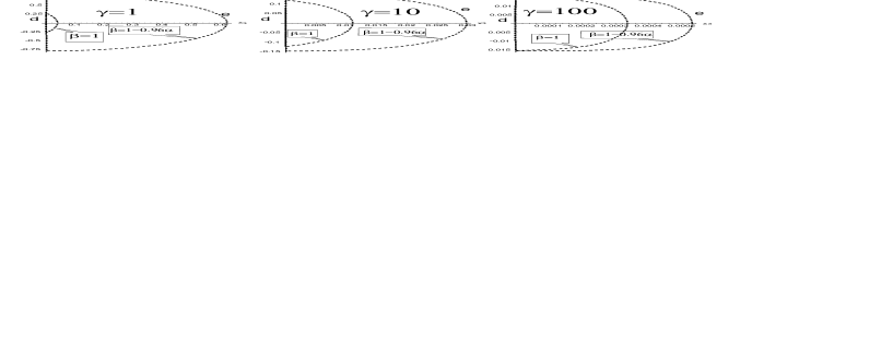
Figure 4: Trajectories in the Euclidean plane $(x_{3},x_{4})$ for various values of parameters $\beta,\gamma$; $\alpha=5\cdot 10^{-3}$, $\frac{m}{eE}$ taken as length unit.

If we calculate the action for these trajectories we will receive a four-parametric expression, depending on $a$, $b$, $u_{0}$ and $v_{0}$. We should find the values of these parameters which minimize the action. One can minimize the action using the standard procedure and taking into account that resulting loop should be closed, i.e. $x_{4}(u_{0})=z_{4}(v_{0})$. Boundary conditions will in this case enter the equations as some constraints with Lagrange multipliers. Instead of this we can use mechanical analogy (see [7]), for which $m$, $M_{d}$ and $M_{m}$ are forces acting in the vertex, so, the minimum of the action corresponds to the value of parameters for which we have equilibrium in the vertex. Condition of the equilibrium is

$$m\cos\alpha_{e}(u_{0})-M_{d}\cos\alpha_{d}(v_{0}) = 0,$$

$$m\sin\alpha_{e}(u_{0})+M_{d}\sin\alpha_{d}(v_{0}) = M_{m}.$$ (5)

$\alpha_{e}(u_{0})$, $\alpha_{d}(v_{0})$ are the inclination angles of corresponding trajectory in the vertex. For the electron we have

$$\tan\alpha_{e}=\sqrt{1+\gamma^{2}}\cot 2\pi u_{0}.$$ (6)

Using analogous relation for dyon and (5) one can easily find

$$\tan^{2}2\pi u_{0} = \left(1+\gamma^{2}\right)\frac{\left((M_{m}+m)^{2}-M_{d}^{2}\right)\left(M_{d}^{2}-(M_{m}-m)^{2}\right)}{\left(m^{2}+M_{m}^{2}-M_{d}^{2}\right)^{2}},$$

$$\tan^{2}2\pi v_{0} = \left(1+\frac{\gamma^{2}}{\alpha^{2}}\right)\frac{\left((M_{m}+m)^{2}-M_{d}^{2}\right)\left(M_{d}^{2}-(M_{m}-m)^{2}\right)}{\left(M_{m}^{2}+M_{d}^{2}-m^{2}\right)^{2}}.$$

It follows immediately from here that for the boundary conditions to be properly satisfied, dyon mass should lie within the interval $M_{m}-m<M_{d}<M_{m}+m$. The action on the extremal trajectory is

$$S_{cl}(\gamma)=S_{e}(\gamma)+S_{d}(\gamma)-2M_{m}x_{4}(u_{0}),$$ (7)

where

$$S_{e}(\gamma) = \frac{1}{\gamma^{2}}\frac{2\pi m^{2}}{eE}\left(2u_{0}\sqrt{1+\gamma^{2}}-\frac{1}{\pi}\arctan\left(\frac{\tan 2\pi u_{0}}{\sqrt{1+\gamma^{2}}}\right)-[2u_{0}+\frac{1}{2}]\right)$$

$$S_{d}(\gamma) = \frac{1}{\gamma^{2}}\frac{2\pi m^{2}}{eE}\left(2v_{0}\sqrt{1+\frac{\gamma^{2}}{\alpha^{2}}}-\frac{1}{\pi}\arctan\left(\frac{\tan 2\pi v_{0}}{\sqrt{1+\frac{\gamma^{2}}{\alpha^{2}}}}\right)-[2v_{0}+\frac{1}{2}]\right),$$

where square brackets $[x]$ in the last expression denote minimal integer part of $x$. For $\sin\alpha_{e,d}>0$, or $\tan 2\pi u_{0}>0$ and $\tan 2\pi v_{0}>0$ (see (6)) i.e. $M_{d}^{2}<m^{2}+M_{m}^{2}$ it follows that

$$u_{0} = \frac{1}{2\pi}\arctan\sqrt{\left(1+\gamma^{2}\right)\frac{\left((M_{m}+m)^{2}-M_{d}^{2}\right)\left(M_{d}^{2}-(M_{m}-m)^{2}\right)}{\left(m^{2}+M_{m}^{2}-M_{d}^{2}\right)^{2}}}<\frac{1}{4},$$

$$v_{0} = \frac{1}{2\pi}\arctan\sqrt{\left(1+\frac{\gamma^{2}}{\alpha^{2}}\right)\frac{\left((M_{m}+m)^{2}-M_{d}^{2}\right)\left(M_{d}^{2}-(M_{m}-m)^{2}\right)}{\left(M_{m}^{2}+M_{d}^{2}-m^{2}\right)^{2}}}<\frac{1}{4},$$

so, the action reads as

$$S_{e}(\gamma) = \frac{1}{\gamma^{2}}\frac{2\pi m^{2}}{eE}\left(2u_{0}\sqrt{1+\gamma^{2}}-\frac{1}{\pi}\arctan\left(\frac{\tan 2\pi u_{0}}{\sqrt{1+\gamma^{2}}}\right)\right),$$

$$S_{d}(\gamma) = \frac{1}{\gamma^{2}}\frac{2\pi m^{2}}{eE}\left(2v_{0}\sqrt{1+\frac{\gamma^{2}}{\alpha^{2}}}-\frac{1}{\pi}\arctan\left(\frac{\tan 2\pi v_{0}}{\sqrt{1+\frac{\gamma^{2}}{\alpha^{2}}}}\right)\right).$$ (8)

For the case $M_{d}^{2}>m^{2}+M_{m}^{2}$ it follows that

$$u_{0}=\frac{1}{2}-\frac{1}{2\pi}\arctan\sqrt{\left(1+\gamma^{2}\right)\frac{\left((M_{m}+m)^{2}-M_{d}^{2}\right)\left(M_{d}^{2}-(M_{m}-m)^{2}\right)}{\left(m^{2}+M_{m}^{2}-M_{d}^{2}\right)^{2}}}>\frac{1}{4}.$$

Corresponding value of the action is

$$S_{e}(\gamma)=\frac{1}{\gamma^{2}}\frac{2\pi m^{2}}{eE}\left(2u_{0}\sqrt{1+\gamma^{2}}-\frac{1}{\pi}\arctan\left(\frac{\tan 2\pi u_{0}}{\sqrt{1+\gamma^{2}}}\right)-1\right).$$ (9)

A family of extremal trajectories for several values of $\gamma$ is shown in Fig. 4. One can see the overall plot of $S(\gamma)$ versus Keldysh parameter $\gamma$ in Fig. 5.

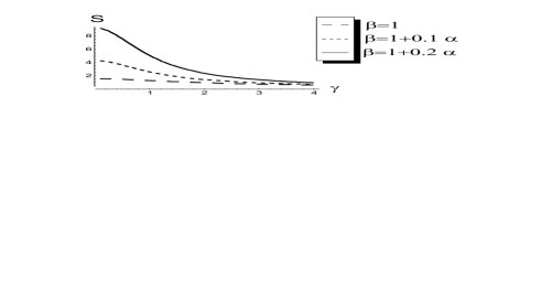
Figure 5: Action $S$ of electron-dyon loop in units of $\frac{m^{2}}{eE}$ versus Keldysh parameter $\gamma$ for temporally inhomogeneous field.

The relation $\frac{\Gamma}{\Gamma_{0}}$, where $\Gamma_{0}$ is monopole mass imaginary part (width) in a constant electric field ($\gamma=0$) can be plotted and is shown in Fig.6. One can easily see the increase of the particle width with the increase of $\gamma$. This increase becomes stronger when the difference between $M_{d}$ and $M_{d}$ grows.

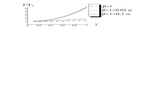
Figure 6: $\frac{\Gamma}{\Gamma_{0}}$ dependence on Keldysh parameter $\gamma$ for temporally inhomogeneous field.

Action $S$ tends to zero as $\gamma\to\infty$, therefore, at some point, resummation of higher winding number contributions  (1) will be necessary. At sufficiently low $S$ the whole process should rather be dealt within common perturbation theory, because semiclassical approximation to the non-perturbative mass shift becomes invalid here.

As it was mentioned in section 2 one has a criterion for applicability of the first quantized approach to dyon and monopole. Namely, the loop should be large enough for dyon to be treated as a point-like object. That is, characteristic loop size, which is about the electronic loop “radius”

$$r_{e}=\left\{\begin{array}[]{l}\frac{1}{\gamma}\frac{m}{eE},\quad\gamma>>1\\ \frac{m}{eE},\quad\gamma<<1\end{array}\right.,$$

should satisfy the condition

$$r_{e}\gg M_{W}^{-1},$$

that is,

$$\begin{array}[]{l}\omega\ll M_{W}\\ \frac{E_{cr}}{E}>>\frac{m}{M_{W}}\end{array}$$

Here $E_{cr}=\frac{m^{2}}{e}$ is the critical field value for electron. For imaginable processes in cosmology, field switch-on rate is obviously less then the enormous 100 GeV $\sim 10^{26}$ Hz, thus in fact the first criterion is always satisfied. The second criterion means that $E<<10^{8}E_{cr}$, which is valid for most of magnetic stars and Reissner-Nordstrom black holes (see section 4).

However, from general arguments it becomes clear [14] that semiclassical approximation is wrong when $S\ll 1$. Therefore, this general limit could give us a more strict criterion of applicability of the formula (7) than monopole size considerations.

3.1 Preexponential: Negative modes

Here we limit ourselves to qualitative considerations. The presence of the zero mode was already discussed and used in the resummation above. We might state, due to the fact that for $\gamma\to 0$ one has a situation, totally analogous to that described in [21]. At sufficiently small $\gamma$ if $M_{d}^{2}<M_{m}^{2}+m^{2}$ one always has one negative dilatational mode, corresponding to overall inflation of the loop. It provides a possibility for monopole mass to acquire an imaginary part. If $M_{d}^{2}>M_{m}^{2}+m^{2}$, another negative mode comes into existence (see [21]), thus making loop contribution to the monopole mass real and describing mass renormalization of a stable monopole. In future, we are going to elaborate a numerical criterion for $\gamma$, below which the above statements are true.

3.2 Spatially inhomogeneous field

Dunne and Schubert have shown [14] that in a spatially inhomogeneous field particle decay probability can be obtained by an analytic continuation of the result for the field with the same temporal inhomogeneity

$$\gamma\to i\gamma.$$ (10)

See also [31, 32] for a more detailed discussion of this analytic continuation procedure. The general fact on spontaneous (induced) processes in spatially inhomogeneous fields is that the imaginary part of the effective action (particle width) decreases with the increase of $\gamma$, becoming zero at some point. Physically one can interpret this fact easily: the field characteristic size becoming too narrow, so that no pair of particles can travel a path long enough to gain energy necessary for leaving the barrier. The explicit formula for the action reads

$$S_{cl}(\gamma)=S_{e}(i\gamma)+S_{d}(i\gamma)-2M_{m}x_{4}(u_{0},i\gamma),$$ (11)

where

$$S_{e}(i\gamma) = \frac{1}{\gamma^{2}}\frac{2\pi m^{2}}{eE}\left(-2u_{0}\sqrt{1-\gamma^{2}}+\frac{1}{\pi}\arctan\left(\frac{\tan 2\pi u_{0}}{\sqrt{1-\gamma^{2}}}\right)\right)$$

$$S_{d}(i\gamma) = \frac{1}{\gamma^{2}}\frac{2\pi m^{2}}{eE}\left(-2v_{0}\sqrt{1-\frac{\gamma^{2}}{\alpha^{2}}}+\frac{1}{\pi}\arctan\left(\frac{\tan 2\pi v_{0}}{\sqrt{1-\frac{\gamma^{2}}{\alpha^{2}}}}\right)\right),$$

Following the simple analytic continuation rule, we show how the exponential factor behaves for field

$$E\sim\frac{1}{\cosh^{2}(\omega x_{3})}.$$ (12)

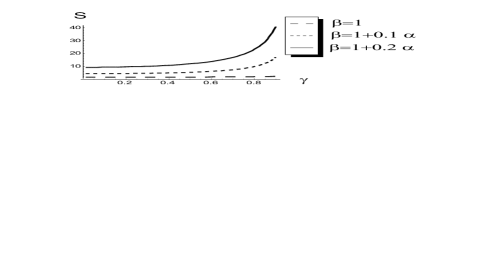
Figure 7: Action $S$ of electron-dyon loop in units of $\frac{m^{2}}{eE}$ versus Keldysh parameter $\gamma$ for spatially inhomogeneous field.

In Fig. 7 one can see that the process of monopole decay becomes infinitely suppressed as $\gamma\to 1$. At higher values of inhomogeneity parameter $\gamma>1$ decay is forbidden. This corresponds fully to the earlier results of [14] for spontaneous pair creation.

Below in Fig.8 we plot the ratio of monopole width in a spatially inhomogeneous field with parameter $\gamma$ to its width in the constant field case.

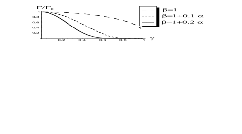
Figure 8: $\frac{\Gamma}{\Gamma_{0}}$ dependence on Keldysh parameter $\gamma$ for spatially inhomogeneous field.

4 Monopoles in Cosmology and High-Energy Physics

The issue of magnetic monopoles, present in almost every 4-dimensional non-abelian gauge theory with a scalar Higgs field  [22, 23] has long been an important problem in high-energy physics. Violation of baryon number conservation law in presence of a magnetic monopole [24], charge quantization [25] are just a few well-known features of rich monopole physics.

One of the problems of monopole physics is the overestimation of monopole concentration in the Universe with regard to experimental limit. E.g. it has been pointed out that our Universe should contain relatively large concentration of free primordial Polyakov – ’t Hooft monopoles of $M\sim M_{W}/\alpha\sim 10^{4}$ GeV (over 10 orders of magnitude larger than the upper experimental bound), unless they are bound in meson-like states or there are alternative mechanisms of monopole decay. GUT monopoles’ ($M\sim 10^{17}$ GeV) generation just after the spontaneous violation of the gauge symmetry of the GUT group was long being thought to be a major trouble for the standard cosmological model, until having been solved in terms of inflationary cosmology in [26].

“Phenomenology” of monopoles nowadays has set some limits on their abundance. The observed flux $J$ on Earth is limited from above as $J<1.4\times 10^{-16}\frac{1}{cm^{2}\,s\,sr}$ [27]. The so-called Parker bound coming from magnetohydrodynamic considerations limits the flux of monopoles by $J<1\times 10^{-15}\frac{1}{cm^{2}\,sec\,sr}$. The expected velocities of the monopoles lie in the range $10^{-4}<v/c<1$, masses of “primordial” GUT monopoles are expected to be of the order of magnitude $10^{17}$ GeV or higher, monopoles with masses $10^{7}\dots 10^{15}$ GeV could have been generated during the later phase transitions (after breaking the GUT symmetry). Lowest ’t Hooft monopole mass is reached in BPS limit $M\sim M_{W}/\alpha$. The limit on concentration of monopoles depends on their velocity and flux, and can roughly be estimated $n_{M}<10^{-26}\cdots 10^{-22}\,cm^{-3}$.

Thus the concentration of monopoles in the Universe is a very important quantity, as we have experimental bounds on it and, on the other hand, the presence of monopoles may have influenced its evolution. Therefore, it is very important to know well the possible channels of monopole decay. In particular, one is interested in external field induced decay processes due to several reasons.

First, one cannot fully eliminate the scenario of monopoles decaying within stellar matter suggested long ago by Zeldovich and Khlopov [28]. One should pay particular attention to these processes in extremal Reissner–Nordstrom black holes, as these objects may create electric fields close to the critical value. (The upper boundary of Reissner–Nordstrom black hole electric field is actually limited from above by $2\times 10^{12}$ Gs [29]). Here one can use constant field limit $\gamma=0$, and the value of the typical action (7) is $S\sim 10$, so that monopole decay is not infinitely suppressed by the factor of $e^{-S}\sim 10^{-4.3}$.

Second, at the start of inflation stage when monopoles had just been born, we may have some non-zero expectation value of (electromagnetic) field, which might have catalyzed monopole decay into something else.

Third, one could consider decay of monopoles in the interstellar media, as it has been argued that magnetic fields of the order of magnitude $10^{-2}$ Gs must exist in dense molecular regions and IR nebulae [30].

Let us estimate realistic values of Keldysh parameter

$$\gamma=\frac{10^{-19}\,sec}{\tau}\frac{E_{cr}}{E}$$

for possible applications of our technique, where $\tau$ is characteristic inhomogeneity time, $E$ typical field value, and $E_{cr}$ critical field value for electron ($4\cdot 10^{13}$ Gs). The most rapid processes observed in the modern Universe have to do with pulsars and can have $\tau\sim 10^{-3}\,sec$. On the other hand, typical magnetic field of a pulsar can reach the order of $10^{-1}E_{cr}$. Thus $\gamma$ is extremely small and one can use the stationary approximation from [21].

In terrestrial conditions, lasers with $\tau\sim 10^{-15}\cdots 10^{-16}$, and $E\sim 10^{-3}\cdots 10^{-5}$ could be within the reach of modern experimentalists. Typical action in this case is $S\sim 10^{3}$, which still suppresses monopole decay. If gamma-lasers could produce pulses short enough, one could hope for diminishing $\tau$ by $2-3$ orders of magnitude and reach values $S\sim 1$. However, such parameters are out of reach at present time. Moreover, the semiclassical approximation breaks down at such values of $S$, as we have mentioned already. Speculating further, one can put a little fantasy in it and conjecture that monopoles could be produced at some high energy facility, and then directed into a device, where the corresponding time-dependent field is created. Then monopole decay into a dyon and an electron could be observed. However, we understand both theoretical and experimental difficulties of implementing such a project. All attempts to detect monopoles at accelerators have failed up to now. E.g., production of (Dirac) monopoles at Tevatron has been considered in [33]. From the data on the existing facilities, bounds upon monopole mass and cross-section have been established: $M>300$ GeV, $\sigma<10^{-37}$ cm². This imposes bounds upon the possible monopole production at, e.g., LHC. If its luminosity be $\sim 10^{34}$ $cm^{-2}s^{-1}$, the upper limit of monopole production would be set as 10⁴ per year, if we rely on the upper bound for cross-section. It is obviously a non-trivial task to detect monopole production itself, and even more complicate done to realize its decay under the conditions assumed in this paper.

5 Discussion

In this short Note the description of the induced monopole decay has been generalized to the non-stationary field case. Comparing to stationary field configuration, one can conclude that, as expected, monopole decay is enhanced by a temporally-inhomogeneous field and suppressed by a spatially inhomogeneous field. It has been shown that, despite being non-perturbatively suppressed, this process may take place under some exotic conditions, e.g. in Reissner–Nordstrom black holes and in pulse gamma or x-ray lasers.

Non-stationarity of field becomes a key factor in the latter case, allowing the classical action on the Euclidean closed worldline to become sufficiently low and thus cease to suppress monopole decay. On the other hand, we have shown that even for the most rapid processes in cosmology, it is generally possible to use constant field approximation from [21].

6 Acknowledgements

Authors are grateful to A. S. Gorsky for suggesting this problem and fruitful discussions. This work is supported in part by 05-01-00992, Scientific School grant NSh-2339.2003.2 and by JINR Heisenberg — Landau project (A.Z.); RFBR 04-01-00646 Grants and Scientific School grant NSh-8065.2006.2 (A.M.).

References

- [1] W. Heisenberg and H. Euler, Z. Phys. 98 (1936) 714.
- [2] J. S. Schwinger, Phys. Rev. 82, 664 (1951).
- [3] I. Y. Kobzarev, L. B. Okun and M. B. Voloshin, Sov. J. Nucl. Phys. 20, 644 (1975) [Yad. Fiz. 20, 1229 (1974)].
- [4] S. R. Coleman, Phys. Rev. D 15, 2929 (1977) [Erratum-ibid. D 16, 1248 (1977)].
- [5] C. G. Callan and S. R. Coleman, Phys. Rev. D 16 (1977) 1762.
- [6] I. K. Affleck and F. De Luccia, Phys. Rev. D 20, 3168 (1979).
- [7] K. Selivanov and M. Voloshin, ZHETP Lett,42 (1985) 422.
- [8] A. Gorsky and M. B. Voloshin, Phys. Rev. D 73, 025015 (2006) [arXiv:hep-th/0511095].
- [9] A. I. Akhiezer and V .B. Berestetskiy, Quantum Electrodynamics [In Russian]. Moscow, 1959, GIFML, 656 pp.
- [10] N. B. Narozhnyi and A. I. Nikishov, Yad. Fiz. 11 (1970) 1072 [Sov. J. Nucl. Phys. 11 (1970) 596].
- [11] V. S. Popov and M. S. Marinov, Yad. Fiz. 16, 809 (1972).
- [12] V. S. Popov, JETP Lett. 74, 133 (2001) [Pisma Zh. Eksp. Teor. Fiz. 74, 151 (2001)].
- [13] I. K. Affleck and N. S. Manton, Nucl. Phys. B 194, 38 (1982).
- [14] G. V. Dunne and C. Schubert, Phys. Rev. D 72, 105004 (2005) [arXiv:hep-th/0507174].
- [15] G. V. Dunne, Q. h. Wang, H. Gies and C. Schubert, Phys. Rev. D 73, 065028 (2006) [arXiv:hep-th/0602176].
- [16] H. M. Fried and R. P. Woodard, Phys. Lett. B 524 (2002) 233 [arXiv:hep-th/0110180].
- [17] G. V. Dunne, arXiv:hep-th/0406216.
- [18] M. K. Parikh and F. Wilczek, Phys. Rev. Lett. 85, 5042 (2000) [arXiv:hep-th/9907001].
- [19] M. Angheben, M. Nadalini, L. Vanzo and S. Zerbini, JHEP 0505, 014 (2005) [arXiv:hep-th/0503081].
- [20] A. S. Gorsky, K. A. Saraikin and K. G. Selivanov, Nucl. Phys. B 628, 270 (2002) [arXiv:hep-th/0110178].
- [21] A. K. Monin, JHEP 0510, 109 (2005) [arXiv:hep-th/0509047].
- [22] A. M. Polyakov, JETP Lett. 20 (1974) 194 [Pisma Zh. Eksp. Teor. Fiz. 20 (1974) 430].
- [23] G. ’t Hooft, Nucl. Phys. B 79, 276 (1974).
- [24] V. A. Rubakov, IYAI-P-0211
- [25] P. A. M. Dirac, Phys. Rev. 74 (1948) 817.
- [26] A. D. Linde, Phys. Lett. B 108, 389 (1982).
- [27] M. Ambrosio et al. [MACRO Collaboration], Eur. Phys. J. C 25, 511 (2002) [arXiv:hep-ex/0207020].
- [28] Y. B. Zeldovich and M. Y. Khlopov, Phys. Lett. B 79 (1978) 239.
- [29] T. Damour and R. Ruffini, Phys. Rev. D 14 (1976) 332.
- [30] C. Heiles, Ann. Rev. Astron. Astrophys. 14 (1976) 1.
- [31] G. V. Dunne and T. Hall, Phys. Rev. D. 58, 105022 (1998).
- [32] M. P. Fry. Phys. Rev. D. 67 065017 (2003).
- [33] G. R. Kalbfleisch, W. Luo, K. A. Milton, E. H. Smith and M. G. Strauss, Phys. Rev. D 69 (2004) 052002 [arXiv:hep-ex/0306045].