Abstract

Transverse-momentum dependent (TMD) light-cone wave functions of a light meson are important ingredients in the TMD QCD factorization of exclusive processes. This factorization allows one conveniently resum Sudakov logarithms appearing in collinear factorization. The TMD light-cone wave functions are not simply related to the standard light-cone wave functions in collinear factorization by integrating them over the transverse momentum. We explore relations between TMD light-cone wave functions and those in the collinear factorization. Two factorized relations can be found. One is helpful for constructing models for TMD light-cone wave functions, and the other can be used for resummation. These relations will be useful to establish a link between two types of factorization.

In the collinear QCD factorization for exclusive processes[1, 2], such as the form factor of $\pi$, the nonperturbative effects are included in various light-cone wave functions. At leading twist, transverse momenta of partons entering a hard scattering are neglected. The hard scattering can be studied in perturbative QCD. In this approach the perturbative expansion for the hard scattering often has large corrections, in the form of large Sudakov double logarithms, around the end-point regions in which one parton in a hadron carries almost all the momentum of the hadron. These large corrections will make perturbative expansions diverge and a resummation is needed for them.

The solution for resumming these corrections is suggested in [3, 4] by taking transverse momenta of partons into account, in which one introduces transverse momentum dependent (TMD) light-cone wave functions similar to the light-cone wave functions in the collinear factorization. We will call the latter as the standard light-cone wave functions. Before a detailed discussion of these wave functions some explanation is needed for the nomenclature. The light-cone wave functions in the collinear factorization here are called quark distribution amplitudes in the pioneer work in [1]. The transverse momentum dependent light-cone wave functions were also introduced in the light-front Hamiltonian formulation of QCD and called as wave functions(see the review [5]). However the TMD light-cone wave functions defined in this letter are slightly different than those wave functions, the difference is because of light singularities and will be discussed later. With the TMD light-cone wave functions one can make a TMD factorization instead of the collinear one and show that the Sudakov logarithms can be resummed. Because the TMD light-cone wave functions are generalizations of the standard ones, one may expect to obtain the standard light-cone wave functions from the TMD ones simply by integrating the transverse momenta. However, this is not the case. In this letter we explore in detail the relationship between these two types of wave functions.

Similar problems also appear in the collinear factorization for inclusive processes like semi-inclusive DIS and Drell-Yan process as well as exclusive $B$-decays, where large corrections appear around edges of kinematical regions. In inclusive processes like Drell-Yan and semi DIS one can introduce TMD parton distributions and a TMD factorization for the differential cross-sections can be obtained[6, 7, 8]. In this formalism one finds that the resummation can be conveniently performed and there is a factorized relation between TMD parton distributions and the distributions appearing in the collinear factorization. In exclusive B-decays, where $b$-quark is described by heavy quark effective theory, the TMD light-cone wave function of $B$-meson can also be consistently defined[9, 10] and its relation to the light-cone wave function in the collinear factorization is explored in [9]. With the TMD light-cone wave function one can show that the TMD factorization for radiative leptonic decay of $B$-meson can be verified at one-loop level and the large correction around the end-point region can be resummed[11]. Using wave functions or TMD light-cone wave functions the form factor of $B\rightarrow\pi$ transition can also be formulated in a factorized form[12]. In other $B$-decays it has been shown that the Sudakov logarithms can be resummed (see e.g., [13] and references therein). It should be pointed out that TMD factorization is not only helpful in resumming large logarithmic corrections but also in probing the 3-dimensional structure of hadrons. Various physical quantities can be represented with these wave functions, e.g., various form factors[14], generalized parton distributions[15], single spin asymmetries[16], etc.

TMD light-cone wave functions can be defined from the matrix elements of quark and gluon operators in QCD. They have been classified in terms of partonic configurations for various hadrons [17]. In the letter we will take $\pi$ as an example, although it is straightforward to extend our results to other hadrons. We will use the light-cone coordinate system, in which a vector $a^{\mu}$ is expressed as $a^{\mu}=(a^{+},a^{-},\vec{a}_{\perp})=((a^{0}+a^{3})/\sqrt{2},(a^{0}-a^{3})/\sqrt{2},a^{1},a^{2})$ and $a_{\perp}^{2}=(a^{1})^{2}+(a^{2})^{2}$. We take $\pi$ with the momentum $P^{\mu}=(P^{+},P^{-},0,0)$ with $P^{+}$ as the large component and introduce a vector $u^{\mu}=(u^{+},u^{-},0,0)$. The TMD light-cone wave function of $\pi$ can be defined as in the limit $u^{+}<<u^{-}$:

$$\phi_{+}(x,k_{\perp},\zeta,\mu) = \ \int\frac{dz^{-}}{2\pi}\frac{d^{2}z_{\perp}}{(2\pi)^{2}}e^{ik^{+}z^{-}-i\vec{z}_{\perp}\cdot\vec{k}_{\perp}}\langle 0|\bar{q}(0)L_{u}^{\dagger}(\infty,0)\gamma^{+}\gamma_{5}L_{u}(\infty,z)q(z)|\pi(P)\rangle|_{z^{+}=0},$$

$$k^{+} = xP^{+},\ \ \ \ \ \zeta^{2}=\frac{2u^{-}(P^{+})^{2}}{u^{+}}\approx\frac{4(u\cdot P)^{2}}{u^{2}},$$ (1)

where $q(x)$ is the light-quark field. We do not specify if the light quark $q$ is a $u$- or $d$-quark and $\pi$ is $\pi^{0}$ or $\pi^{+}$, which is not important for our discussion. $L_{u}$ is the gauge link in the direction $u$:

$$L_{u}(\infty,z)=P\exp\left(-ig_{s}\int_{0}^{\infty}d\lambda u\cdot G(\lambda u+z)\right).$$ (2)

It should be understood that the contributions proportional to any positive power of $u^{+}/u^{-}$ are neglected. This definition was first proposed in [3]. It is gauge invariant in any non-singular gauge in which the gauge field is zero at infinite space-time. The TMD wave function has an extra variable $\zeta^{2}$ beside the momentum faction $x$, the transverse momentum $k_{\perp}$ and the renormalization scale $\mu$. The evolution of this variable will generate the resummed Sudakov logarithms as shown in [3]. This will be confirmed in this letter. The evolution with the renormalization scale $\mu$ is simple:

$$\mu\frac{\partial\phi_{+}(x,k_{\perp},\zeta,\mu)}{\partial\mu}=2\gamma_{q}\phi_{+}(x,k_{\perp},\zeta,\mu),$$ (3)

where $\gamma_{q}$ is the anomalous dimension of the light quark field $q$ in the axial gauge $u\cdot G=0$. In the axial gauge, the gauge links in our definition disappear. Some general features of TMD light-cone wave functions defined by using the light-cone gauge link with $u^{+}=0$ have been studied in [18, 19]. In [18] the operator product expansion was employed to analyze the short distance behavior of wave functions. However, the TMD light-cone wave functions defined with $u^{+}=0$ will have light-cone singularities like $1/(1-x)$, as pointed out in [20] for TMD parton distributions. We will also show through our calculation that these singularities exist if one sets $u^{+}=0$ at the beginning. With a finite, but large $\zeta$, the light-cone singularities are regularized. Because of the small but finite $u^{+}$, the TMD light-cone wave function is not the wave function introduced in the light-front Hamiltonian formulation of QCD[5]. However, with our definition one can still derive the so-called Drell-Yan-West relation(See [23]), which shows that the behavior of the TMD light-cone wave function of a hadron in the region of $x\rightarrow 1$ is related to the structure function of the hadron in the region of $x\rightarrow 1$ and the leading power behavior of the form factor factor of the hadron. With the definition of TMD light-cone wave function it has already been shown that the TMD factorization for the form factor in the transition of $\gamma^{*}\pi\rightarrow\gamma$ can be consistently factorized at least at one-loop level[21]. It should be noted that the TMD light-cone wave function defined in Eq.(1) is real. This can be shown by using parity- and time-reversal transformation and with the fact that the TMD light-cone wave function depends on the vector $u$ through $\zeta^{2}$.

The standard light-cone wave function is defined as[1]:

$$\Phi_{+}(x,\mu)=\int\frac{dz^{-}}{2\pi}e^{ik^{+}z^{-}}\langle 0|\bar{q}(0)L_{n}^{\dagger}(\infty,0)\gamma^{+}\gamma_{5}L_{n}(\infty,z)q(z)|\pi(P)\rangle|_{z^{+}=0,\vec{z}_{\perp}=0},$$ (4)

where the gauge link is along the light-cone direction $n^{\mu}=(0,1,0,0)$. Comparing the two definitions one would expect in the limit $u^{+}\rightarrow 0$ that the standard light-cone-wave function can be obtained by:

$$\Phi_{+}(x,\mu)=\int d^{2}k_{\perp}\phi_{+}(x,k_{\perp},\zeta,\mu),$$ (5)

where the integration over $k^{2}_{\perp}$ is from $0$ to $\infty$. However, this is not true. The reason is as follows: By the generalized power counting rule [22], $\phi_{+}$ is proportional to $k^{-2}_{\perp}$ as $k^{2}_{\perp}\rightarrow\infty$. Hence the transverse momentum integral is ultraviolet (U.V.) divergent. In Eq.(4) the integration over the transverse momentum is supplemented with systematic U.V. subtractions and this generates a renormalization scale dependence in $\Phi_{+}$. This leads to the Efremov-Radyushkin-Brodsky-Lepage evolution equation[24]. In the above integration one may also implement an U.V. subtraction by introducing a suitable cut-off for $k_{\perp}$. This is easy to do at one-loop level, and but difficult to extend beyond one-loop. Also the limit $u^{+}\rightarrow 0$ or $\zeta\rightarrow\infty$ is nontrivial.

Although it is tricky to establish the above relation, the two types of wave functions are related to each other in other ways. If we transform the TMD light-cone wave function into the impact space

$$\phi_{+}(x,b,\zeta,\mu)=\int d^{2}k_{\perp}e^{i\vec{k}_{\perp}\cdot\vec{b}}\phi_{+}(x,k_{\perp},\zeta,\mu)$$ (6)

it can be shown that a factorized relation exists between two wave functions if $b$ is small:

$$\phi_{+}(x,b,\zeta,\mu)=\int_{0}^{1}dyC_{b}(x,y,\zeta,b,\mu)\Phi_{+}(y,\mu)+{\mathcal{O}}(b),$$ (7)

where the function $C$ can be calculated in perturbative QCD and does not have any soft divergence. When $b$ is small, it corresponds to a large momentum scale, and hence its dependence must be calculable in perturbation theory. $\zeta$ can be understood as a large scale, its dependence shall also be perturbative. The factorization theorem asserts that all nonperturbative effect in $\phi_{+}(x,b,\zeta,\mu)$ is resided in $\Phi_{+}(x,\mu)$ for small $b$. We will show this is true at one-loop level and our result can be extended beyond one-loop.

Another interesting relation can be found if $k_{\perp}$ is large, which can be generated by exchanges of gluons between partons inside $\pi$ and these gluons are hard. Hence the behavior at large $k_{\perp}$ can be studied with perturbative QCD. One expects the type of factorization:

$$\phi_{+}(x,k_{\perp},\zeta,\mu)=\frac{1}{k_{\perp}^{2}}\int_{0}^{1}dyC_{\perp}(x,y,\zeta,\mu)\Phi_{+}(y,\mu)+{\mathcal{O}}(k^{-4}_{\perp}).$$ (8)

The factor $k^{-2}_{\perp}$ is determined by the power counting rule in [22].

As discussed above, the two functions $C_{b}$ and $C_{\perp}$ can be calculated in perturbative QCD. To do that, we take a partonic state to calculate the two wave functions at one-loop order, in which we have both infrared- and collinear divergences. We regularize infrared divergences by taking a small gluon mass $\lambda$, and collinear divergences by taking a small quark mass $m_{q}$. If the factorization in Eq.(7) is correct, $C_{b}$ will have no singular dependence on these small masses. It should be noted that our results for the two wave functions at one-loop level will also be useful to establish TMD- and collinear factorization theorems for exclusive processes at one-loop. We take the partonic state $|q(k_{q}),\bar{q}(k_{\bar{q}})\rangle$ to replace $\pi$ in the above definitions, the parton momenta are given as

$$k_{q}^{\mu}=(k_{q}^{+},k_{q}^{-},\vec{k}_{q\perp}),\ \ \ \ k_{\bar{q}}^{\mu}=(k_{\bar{q}}^{+},k_{\bar{q}}^{-},-\vec{k}_{q\perp}),\ \ \ \ \ \ k_{q}^{+}=x_{0}P^{+},\ \ \ \ k_{\bar{q}}^{+}=(1-x_{0})P^{+}=\bar{x}_{0}P^{+}.$$ (9)

These partons are on-shell. At tree-level the wave functions are trivial:

$$\phi_{+}^{(0)}(x,k_{\perp},\zeta)=\delta(x-x_{0})\delta^{2}(\vec{k}_{\perp}-\vec{k}_{q\perp})\phi_{0},\ \ \ \ \ \Phi_{+}^{(0)}(x,\mu)=\delta(x-x_{0})\phi_{0},$$ (10)

where $\phi_{0}$ is a product of spinors $\phi_{0}=\bar{v}(k_{\bar{q}})\gamma^{+}\gamma_{5}u(k_{q})/P^{+}$. We will always write a quantity $A$ as $A=A^{(0)}+A^{(1)}+\cdots$, where $A^{(0)}$ and $A^{(1)}$ stand for tree-level- and one-loop contribution respectively.

At one-loop level, one can divide the corrections into a real part and a virtual part. The real part comes from contributions of Feynman diagrams given in Fig.1. The virtual part comes from contributions of Feynman diagrams given in Fig.2, which are proportional to the tree-level result.

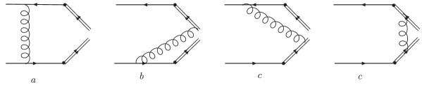
Figure 1: The real part of one-loop contribution to the TMD light-cone wave function. The double lines represent the gauge links.

The contribution from Fig.1b and Fig.1c and Fig.1d to $\phi_{+}$ reads:

$$\phi_{+}(x,k_{\perp},\zeta)|_{1b} = -\frac{2\alpha_{s}}{3\pi^{2}}\left\{\theta(x_{0}-x)\left(\frac{1}{x-x_{0}}\right)_{+}\frac{x}{x_{0}\Delta_{q}}+\frac{1}{2}\delta(x-x_{0})\frac{1}{q_{\perp}^{2}+\lambda^{2}}\ln\frac{q_{\perp}^{2}+\lambda^{2}}{\zeta^{2}x_{0}^{2}}\right\}\phi_{0},$$

$$\Delta_{q} = (1-y)^{2}m_{q}^{2}+y\lambda^{2}+(k_{\perp}-yk_{q\perp})^{2},\ \ \ y=\frac{x}{x_{0}},\ \ \ \ q_{\perp}=k_{\perp}-k_{q\perp},$$

$$\phi_{+}(x,k_{\perp},\zeta)|_{1c} = \frac{2\alpha_{s}}{3\pi^{2}}\left\{\theta(x-x_{0})\left(\frac{1}{x-x_{0}}\right)_{+}\frac{1-x}{(1-x_{0})\Delta_{\bar{q}}}-\frac{1}{2}\delta(x-x_{0})\frac{1}{q_{\perp}^{2}+\lambda^{2}}\ln\frac{q_{\perp}^{2}+\lambda^{2}}{\zeta^{2}\bar{x}_{0}^{2}}\right\}\phi_{0},$$

$$\Delta_{\bar{q}} = \left(1-\bar{y}\right)^{2}m_{q}^{2}+\bar{y}\lambda^{2}+\left(k_{\perp}-\bar{y}k_{q\perp}\right)^{2},\ \ \ \bar{y}=\frac{\bar{x}}{\bar{x}_{0}},$$

$$\phi_{+}(x,k_{\perp},\zeta)|_{1d} = -\frac{2\alpha_{s}}{3\pi^{2}}\frac{1}{\lambda^{2}+q^{2}_{\perp}}\delta(x-x_{0})\phi_{0},$$ (11)

where we have already taken the limit $\zeta\rightarrow\infty$ and only kept the leading terms. If we set $u^{+}=0$ or $\zeta=\infty$ at the beginning, the contribution from Fig.1b and Fig.1c will be divergent as $(x-x_{0})^{-1}$ when $x\rightarrow x_{0}$, and Fig.1d will not lead nonzero contribution. The divergence is the light-cone singularity mentioned before, caused by the exchanged gluon if it has the momentum $k_{g}^{\mu}=(k_{g}^{+},k_{g}^{-},\vec{k}_{g\perp})$ with a vanishing small $k_{g}^{+}$. With a finite, but large $\zeta$ the divergence is regularized. It results in the $+$-distributions and the terms with $\ln\zeta$ in the above expressions. From the above results one clearly sees that there are collinear- and infrared singularities when transverse momenta are small. It should be noted that the contributions from Fig.1b and Fig.1c are related to each other by charge-conjugation.

The contribution from Fig.1a is complicated. But for the function $C_{\perp}$ and $C_{b}$ we only need the leading part of the contribution with $k_{\perp}\rightarrow\infty$. The leading part can be written as: which is

$$\phi_{+}(x,k_{\perp},\zeta)|_{1a} = \frac{2\alpha_{s}}{3\pi^{2}}\frac{1}{k_{\perp}^{2}+\Lambda^{2}}\left(\frac{x}{x_{0}}\theta(x_{0}-x)+\frac{1-x}{1-x_{0}}\theta(x-x_{0})\right)\phi_{0}$$ (12)

$$+"finite\ terms",$$

where we introduce a ”cut-off” $\Lambda$, which is also contained in the second line, so that the total does not depend on it. The second line behaves like $k^{-4}_{\perp}$ with $k_{\perp}\rightarrow\infty$. One can show that the second line is irrelevant here, but it is relevant to what is neglected in Eq.(7,8).

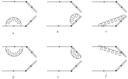
Figure 2: The virtual part of one-loop contribution to the TMD light-cone wave function. The double lines represent the gauge links.

The virtual part of the one-loop correction is from the Feynman diagrams given in Fig.2. Contributions from each diagrams are:

$$\phi_{+}(x,k_{\perp},\zeta)|_{2a} = \phi_{+}(x,k_{\perp},\zeta)|_{2d}=\phi_{+}^{(0)}(x,k_{\perp},\zeta)\cdot\frac{\alpha_{s}}{6\pi}\left[-\ln\frac{\mu^{2}}{m_{q}^{2}}+2\ln\frac{m_{q}^{2}}{\lambda^{2}}-4\right],$$

$$\phi_{+}(x,k_{\perp},\zeta)|_{2b} = \phi_{+}(x,k_{\perp},\zeta)|_{2e}=\phi_{+}^{(0)}(x,k_{\perp},\zeta)\cdot\frac{\alpha_{s}}{3\pi}\ln\frac{\mu^{2}}{\lambda^{2}},$$

$$\phi_{+}(x,k_{\perp},\zeta)|_{2c} = \phi_{+}^{(0)}(x,k_{\perp},\zeta)\cdot\frac{\alpha_{s}}{6\pi}\left[2\ln\frac{\mu^{2}}{m_{q}^{2}}+2\ln\frac{\zeta^{2}x_{0}^{2}}{m_{q}^{2}}+\ln^{2}\frac{m_{q}^{2}}{\lambda^{2}}-\ln^{2}\frac{\zeta^{2}x_{0}^{2}}{\lambda^{2}}-\frac{2\pi^{2}}{3}+4\right],$$

$$\phi_{+}(x,k_{\perp},\zeta)|_{2f} = \phi_{+}(x,k_{\perp},\zeta)|_{2c}|_{x_{0}\rightarrow\bar{x}_{0}}.$$ (13)

These results also contain collinear- and infrared divergences. The complete one-loop contribution $\phi_{+}^{(1)}$ is the sum of contributions from the 10 Feynman diagrams in Fig.1. and Fig.2. From the above one-loop result one can already obtain the relation in Eq.(8) with the function $C_{\perp}$ determined as:

$$C_{\perp}(x,y,\zeta,\mu) = \frac{2\alpha_{s}}{3\pi^{2}}\left\{-\theta(y-x)\left[\left(\frac{x}{y}\frac{1}{x-y}\right)_{+}-\frac{x}{y}\right]+\theta(x-y)\left[\left(\frac{1-x}{1-y}\frac{1}{x-y}\right)_{+}+\frac{1-x}{1-y}\right]\right.$$ (14)

$$\left.+\delta(x-y)\left[\ln\frac{k_{\perp}^{2}}{\zeta^{2}}+\ln(1-x)^{2}+\ln x^{2}-1\right]\right\}+{\mathcal{O}}(\alpha_{s}^{2}).$$

In the above the $+$-prescription acts on the distribution variable $y$. We have used the identity

$$\left(\frac{x}{y}\frac{\theta(y-x)}{x-y}\right)_{+}=\left(\frac{x}{y}\frac{\theta(y-x)}{x-y}\right)_{+}-\delta(x-y)\left[1+\ln(1-x)\right],$$ (15)

where the $+$-prescription in the left hand side acts on the distribution variable $x$, while the $+$-prescription in the right hand side acts on the distribution variable $y$,

To derive the relation in Eq.(7) one needs to transform the above results into the impact parameter space and to obtain one-loop results of $\Phi_{+}$. The Fourier transformation can be done straightforwardly. We find that there is a cancelation of infrared divergence between the real- and virtual part correspondingly. We present our results in the combination in which infrared divergences are canceled:

$$\phi_{+}(x,b,\zeta,\mu)|_{1b+2c} = \frac{2\alpha_{s}}{3\pi}\phi_{0}\left\{\frac{1}{4}\delta(x-x_{0})\left[-\ln^{2}(\tilde{b}^{2}\zeta^{2}x_{0}^{2})+2\ln(\tilde{b}^{2}\mu^{2})+2\ln(\tilde{b}^{2}\zeta^{2}x_{0}^{2})-4-\pi^{2}\right]\right.$$

$$\left.+\theta(x_{0}-x)\left[\frac{x}{x_{0}}\frac{\ln(\tilde{b}^{2}m_{q}^{2}(1-y)^{2})}{x-x_{0}}\right]_{+}\right\}+{\mathcal{O}}(b),$$

$$\phi_{+}(x,b,\zeta,\mu)|_{1c+2f} = \frac{2\alpha_{s}}{3\pi}\phi_{0}\left\{\frac{1}{4}\delta(x-x_{0})\left[-\ln^{2}(\tilde{b}^{2}\zeta^{2}\bar{x}_{0}^{2})+2\ln(\tilde{b}^{2}\mu^{2})+2\ln(\tilde{b}^{2}\zeta^{2}\bar{x}_{0}^{2})-4-\pi^{2}\right]\right.$$

$$\left.-\theta(x-x_{0})\left[\frac{1-x}{1-x_{0}}\frac{\ln(\tilde{b}^{2}m_{q}^{2}(1-\bar{y})^{2})}{x-x_{0}}\right]_{+}\right\}+{\mathcal{O}}(b),$$

$$\phi_{+}(x,b,\zeta,\mu)|_{1d+2b+2e} = \frac{2\alpha_{s}}{3\pi}\phi_{0}\delta(x-x_{0})\ln(\tilde{b}^{2}\mu^{2})+{\mathcal{O}}(b),$$ (16)

with $\tilde{b}=be^{\gamma}/2$. The contribution from Fig.2a and Fig.2d in the b-space can be easily read off from Eq.(15) With these results in the $b$-space one can derive the evolution of $\zeta$:

$$\zeta\frac{\partial}{\partial\zeta}\phi_{+}(x,b,\zeta,\mu) = \left[-\frac{2\alpha_{s}}{3\pi}\ln\frac{\zeta^{2}x^{2}b^{2}e^{2\gamma-1}}{4}-\frac{2\alpha_{s}}{3\pi}\ln\frac{\zeta^{2}(1-x)^{2}b^{2}e^{2\gamma-1}}{4}\right]\phi_{+}(x,b,\zeta,\mu)+{\mathcal{O}}(\alpha_{s}^{2})$$ (17)

$$= -\frac{4\alpha_{s}}{3\pi}\left[\ln(\tilde{b}^{2}\mu^{2})+\ln\frac{\zeta^{2}x(1-x)}{e\mu^{2}}\right]\phi_{+}(x,b,\zeta,\mu)+{\mathcal{O}}(\alpha_{s}^{2}).$$

This equation was derived first in [3]. Our result agrees with that in [3]. The solution of the equation will contain the Sudakov logarithms in a resummed form.

The one-loop contributions to $\Phi_{+}$ are represented by the same diagrams given in Fig.1 and Fig.2, except those in which the gluon is exchanged between gauge links. Some of them contains light-cone singularities because the gauge link is along the direction $n$, i.e., $u^{+}=0$ is set at the beginning. This singularity is canceled between the real- and virtual part correspondingly. We present our results in the combination free from the singularity:

$$\Phi_{+}(x,\mu)|_{1c}+\Phi_{+}(x,\mu)|_{2f} = -\frac{2\alpha_{s}}{3\pi}\phi_{0}\theta(x-x_{0})\left[\frac{1-x}{(1-x_{0})(x-x_{0})}\ln\frac{m_{q}^{2}(1-\bar{y})^{2}}{\mu^{2}}\right]_{+},$$

$$\Phi_{+}(x,\mu)|_{1b}+\Phi_{+}(x,\mu)|_{2c} = \frac{2\alpha_{s}}{3\pi}\phi_{0}\theta(x_{0}-x)\left[\frac{x}{x_{0}(x-x_{0})}\ln\frac{m_{q}^{2}(1-y)^{2}}{\mu^{2}}\right]_{+}.$$ (18)

Again, the contribution to $\Phi_{+}$ from Fig.1a is complicated. However the relevant part is just by integrating the leading part of $\phi_{+}|_{1a}$ over $k_{\perp}$ with dimensional regularization. We have the relevant part as:

$$\Phi_{+}(x,\mu)|_{1a} = \frac{2\alpha_{s}}{3\pi}\phi_{0}\left(\ln\frac{\mu^{2}}{\Lambda^{2}}-1\right)\left[\frac{x}{x_{0}}\theta(x_{0}-x)+\frac{1-x}{1-x_{0}}\theta(x-x_{0})\right]$$ (19)

$$+"finite\ terms",$$

where the factor $-1$ comes from manipulation of $\gamma$-matrices in $d$-dimension.

With the above results we can extract the function $C_{b}(x,y,\zeta,b,\mu)$. At tree-level

$$C_{b}^{(0)}(x,y,\zeta,b,\mu)=\delta(x-y).$$ (20)

At one-loop we have:

$$C_{b}^{(1)}(x,y,\zeta,b,\mu) = \frac{2\alpha_{s}}{3\pi}\left\{-\left(\ln(\tilde{b}^{2}\mu^{2})-1\right)\left[\frac{x}{y}\theta(y-x)+\frac{1-x}{1-y}\theta(x-y)\right]\right.$$ (21)

$$\left.+\frac{1}{4}\delta(x-y)\left[-\ln^{2}(\tilde{b}^{2}\zeta^{2}y^{2})-\ln^{2}(\tilde{b}^{2}\zeta^{2}(1-y)^{2})-8-2\pi\right.\right.$$

$$\left.\left.-2(\ln y^{2}+\ln(1-y)^{2})\ln(\tilde{b}^{2}\mu^{2})+2\ln(\tilde{b}^{2}\zeta^{2}y^{2})+2\ln(\tilde{b}^{2}\zeta^{2}(1-y)^{2})\right]\right.$$

$$\left.+\theta(y-x)\left[\frac{x}{y}\frac{\ln(\tilde{b}^{2}\mu^{2})}{x-y}\right]_{+}-\theta(x-y)\left[\frac{1-x}{1-y}\frac{\ln(\tilde{b}^{2}\mu^{2})}{x-y}\right]_{+}\right\}.$$

In the above the $+$-prescription acts on the variable $y$. Clearly, it is free from any collinear- or infrared singularity as expected.

To summarize: In this letter we have performed a study of the TMD light-cone wave function of a $\pi$ meson which appears in TMD factorization of exclusive processes. We have established two factorized relations between the TMD- and the standard light-cone wave function, the latter is relevant in collinear factorization of exclusive processes. One relation is that the TMD light-cone wave function can be written as a convolution of the standard one with a perturbative coefficient function $C_{\perp}$ when the transverse momentum is large. This relation is helpful for constructing models of the TMD light-cone wave function. Another is that the TMD light-cone wave function in the impact parameter $b$ space can be written as a convolution of the standard one with a perturbative coefficient function $C_{b}$ when $b$ is small. The function $C_{b}$ contains only perturbative effect and is determined at one-loop level. This factorized relation can be extended beyond one-loop level and it is useful for resummation of Sudakov logarithms. From our results we confirm the result of the evolution equation of $\zeta$, first derived in [3]. The solution of the equation resums the large Sudakov logarithms.

Acknowledgments

The authors thank Prof. X.D. Ji for reading the manuscript. This work is supported by National Nature Science Foundation of P.R. China.

References

• [1] G.P. Lepage and S.J. Brodsky, Phys. Rev. D22 (1980) 2157.
• [2] V.L. Chernyak and A. R. Zhitnitsky, Phys. Rept. 112 (1984) 173.
• [3] J. Botts and G. Sterman, Nucl. Phys. B325 (1989) 62.
• [4] H.-n. Li and Sterman, Nucl. Phys. B381 (1992) 129.
• [5] S.J. Brodsky, H.-C. Pauli, S.S. Pinsky, Phys. Rept. (1998) 299.
• [6] J.C. Collins and D.E. Soper, Nucl. Phys. B193 (1981) 381[Erratum-ibid. B213 (1983) 545], Nucl. Phys. B197 (1982) 446.
• [7] J.C. Collins, D.E. Soper and G. Sterman, Nucl. Phys. B250 (1985) 199.
• [8] X.D. Ji, J.P. Ma and F. Yuan, Phys. Rev. D71 (2005) 034005, hep-ph/0404183, Phys. Lett. B597 (2004) 299,hep-ph/0405085, JHEP 0507 (2005)020,hep-ph/0503015.
• [9] J.P. Ma and Q. Wang, Phys. Lett. B613 (2005) 39, hep-ph/0412282
• [10] H.-n. Li and H.-S. Liao, Phys. Rev. D70 (2004) 074030.
• [11] J.P. Ma and Q. Wang, JHEP 0601 (2006) 067, hep-ph/0510336.
• [12] S.J. Brodsky, D.S. Hwang, Nucl.Phys. B543(1999) 239.
• [13] H.-n. Li and H.-L. Yu, Phys. Rev. D53 (1996) 2480-2490,1996, hep-ph/9411308, C.-H. Chen, Y.-Y. Keum and H.-n Li, Phys.Rev. D66 (2002) 054013,hep-ph/0204166, Phys.Rev.D64:112002,2001 e-Print Archive: hep-ph/0107165, X.-Q Yu, Y. Li and C.-D. LΓΌ, Phys.Rev. D73 (2006) 017501, hep-ph/0511269.
• [14] S.J. Brodsky, D. S. Hwang, B.-Q. Ma, I. Schmidt, Nucl.Phys. B593 (2001) 311, hep-th/0003082
• [15] M. Diehl, T. Feldmann, R. Jakob, P. Kroll, Nucl.Phys. B596 (2001) 33 Erratum-ibid. B605 (2001) 647, hep-ph/0009255
• [16] S.J. Brodsky, D.S. Hwang and I. Schmidt, Nucl.Phys. B642 (2002) 344, hep-ph/0206259
• [17] X.D. Ji, J.P. Ma and F. Yuan, Nucl. Phys. B652 (2003) 383, hep-ph/0210430, Eur. Phys. J. C33 (2004) 75, hep-ph/0304107
• [18] S.J. Brodsky, Y. Frishman, G.P. Lepage and C. Sachrajda, Phys. Lett. B91 (1980) 239.
• [19] B. Chibisov and A. R.Β Zhitnitsky, Phys. Rev. D52 (1995) 5273, hep-ph/9503476.
• [20] J.C. Collins, Acta. Polon. B34 (2003) 3103.
• [21] J.P. Ma and Q. Wang, hep-ph/0607234.
• [22] X.D. Ji, J.P. Ma and F. Yuan, Phys. Rev. Lett. 90 (2003) 241601, hep-ph/0301141.
• [23] F.E. Close, ”An Introduction to Quark and Partons”, Academic Press, 1979.
• [24] S. Brodsky and G.P. Lepage, Phys. Lett. B87 (1979) 359, A.V. Efremov and A.V. Radyushkin, Phys. Lett. B94 (1980) 245.