It’s a Gluino!

Abstract

For a long time it has been known that the like–sign dilepton signature can help establish the existence of a gluino at the LHC. To unambiguously claim that we see a strongly interacting Majorana fermion — which we could call a gluino — we need to prove that it is indeed a fermion. We propose how to extract this information from a different gluino decay cascade which is also used to measure its mass. Looking only at angular correlations we distinguish a universal extra dimensional interpretation assuming a bosonic heavy gluon from supersymmetry with a fermionic gluino. Assuming a supersymmetric interpretation, we show how the same angular correlations can be used to study the left–right nature of the sfermions appearing in the decay chain.

.1 Introduction

Signals for new physics at hadron colliders largely rely on the production and decay of strongly interacting new particles, e.g. in the case of supersymmetry susy the production of squarks and gluinos deq ; prospino with their subsequent decays. Based on this simple fact, it is obvious how to inclusively search for these particles: if the lightest supersymmetric partner is neutral and stable, squarks and gluinos have to decay to (at least) one or two jets and missing transverse momentum $/\!\!\!p_{T}$.

Once we require one charged lepton in the squark or gluino decay we can start testing properties of SUSY–QCD: like–sign dileptons can for example be produced in quark–quark scattering $qq\to\tilde{q}\tilde{q}$ via a $t$–channel gluino. This process requires fermion–number violating interactions of the gluino, i.e. it is a sign for the Majorana nature of the $t$–channel fermion. Like–sign dileptons also appear in gluino pair production $q\bar{q}/gg\to\tilde{g}\tilde{g}$, when the Majorana gluino decays to $q\tilde{q}^{*}$ or $\bar{q}\tilde{q}$ and the squark/antisquark decay yields one definite–charge lepton likesign . The advantage of this SUSY-QCD signature is that the signal process is strongly interacting, while the (non-misidentification) backgrounds are multiple $W$ and $Z$ boson production, i.e. weakly interacting or multi–top induced. At the LHC pairs of $500~{}{\rm GeV}$ gluinos are copiously produced, with cross sections of ${\cal O}(50~{}{\rm pb})$ (not counting the large associated $\tilde{q}\tilde{g}$ production channel) prospino . Therefore, there is little doubt that we will be able to extract this like–sign dilepton signature even if its branching ratio is small.

Motivated by electroweak baryogenesis and its requirement for light stops, there is a variation of this like–sign dilepton signature sabine , namely the decay $\tilde{g}\to t\tilde{t}_{{1}}^{*}/\bar{t}\tilde{t}_{{1}}$ decay_st . Because the stop decays $\tilde{t}\to b\tilde{\chi}^{+}_{{1}}\to bW^{+}\tilde{\chi}^{0}_{{1}}$ and $\tilde{t}\to t\tilde{\chi}^{0}_{{1}}$ are irreducible from a top decay, the like–sign dileptons gluino events will look just like Standard Model $t\bar{t}t\bar{t}$ production, except with an increased rate and possibly different angular correlations.

This recipe for using the like–sign dilepton signature to show that new physics at the LHC incorporates a strongly interacting Majorana fermion and is, therefore, likely to be SUSY–QCD unfortunately has a loop hole. If the particle responsible for a gluino–like cascade decay is a boson ued ; early with an adjoint color charge, the like–sign dilepton signature will naturally occur: two such bosons will each decay into either a ‘squark–antisquark’ pair or even into a simple Standard Model $t\bar{t}$ pair and thus produce like–sign dileptons.

To close this loop hole we need to show that the strongly interacting particle responsible for our like–sign dilepton events is indeed a fermion. Depending on the supersymmetric mass spectrum, the gluino mass can be precisely determined in the (not like–sign dilepton) cascade decay $\tilde{g}\to b\tilde{b}_{{1}}^{*}/\bar{b}\tilde{b}_{{1}}$, where the light sbottom decays through the long chain $\tilde{b}_{{1}}\to\tilde{\chi}^{0}_{{2}}\to\tilde{\ell}\to\tilde{\chi}^{0}_{{1}}$ edges ; mgl . The two decay chains would then have to be linked by comparing their detailed decay kinematics. In the similar case of a $\tilde{q}_{{L}}$ decay we know how to show that the starting point of that cascade is indeed a scalar barr ; smillie . To do so, the strategy includes a few crucial steps: first, we assume (and for gluino decays with bottom tags we know) that all outgoing Standard Model particles in the cascade decay are fermions. In other words, the intermediate particles in the cascade have to alternate between fermions and bosons. To determine the spin nature of the heavy SUSY–QCD particle all we have to do is compare the SUSY cascade with another scenario where the new intermediate states have the same spin as the Standard Model particles instead. Such a model are Universal Extra Dimensions (UED) ued where each Standard Model particle has a heavy Kaluza–Klein (KK) partner which can mimic the SUSY cascade decay, provided the mass spectra which can be extracted from the decay kinematics match early .

There are many observables which we can use to discriminate ‘typical’ UED and SUSY models, like the production rate smillie , ratios of branching fractions or the mass spectrum. At the LHC we measure only production cross sections times branching ratios times efficiencies with fairly large errors. In particular in the supersymmetric squark sector rate information can be diluted through the existence of several strongly interacting scalars with similar decays. Moreover, the UED as well as the SUSY mass spectra might well to be what we currently consider ‘typical’. On the other hand, direct spin information is generally extracted from angular correlations. This kinematic information should at the end be combined with rate information. Because these two approaches are independent of each other we base our analysis exclusively on distributions of the outgoing Standard Model fermions as predicted by UED and by SUSY for a well–established decay chain. All masses in the decay cascade we assume to be measured from the kinematic endpoints of the same set of distributions. Because angles are not Lorentz invariants, it is much easier to interpret invariant masses like $m_{\ell q},m_{\ell\ell}$ barr . Boosting the laboratory frame into the rest frame of for example the $\tilde{\chi}^{0}_{{2}}$ we can (on the generator level) translate invariant masses and angles into each other. The only angles which are independent of the unknown over-all event boost in the beam direction are azimuthal opening angles, e.g. between the two bottom jets $\phi_{bb}$, whose distinguishing power we will discuss in a separate section.

If we knew which of the leptons in the $\tilde{q}_{{L}}$ decay chain is the one radiated right after the quark (the near lepton), i.e. if we could link $\ell^{+/-}$ and $\ell^{\rm near/far}$ edges ; barr ; smillie , we could simply compare $m_{q\ell}$ mass distributions to distinguish UED from SUSY cascades. In practice, we have to find a way to not symmetrize over $\ell^{+}$ and $\ell^{-}$ or $q$ and $\bar{q}$. The trick used for the $\tilde{q}_{{L}}$ cascade is to rely on the fact that squarks are largely produced in association with a gluino ($pp\to\tilde{q}_{{L}}\tilde{g}$), and that squark cascade decays will preferably produce $q$ and not $\bar{q}$ jets, even though on an event-by-event basis we cannot distinguish the two smillie .

Because of the like–sign dilepton argument described above, we are much more interested in the spin of the gluino than in the spin of a squark. Luckily, for the determination of the gluino spin we can almost completely follow the squark spin argument, with the exception of the last trick — a Majorana gluino will always average over $q$ and $\bar{q}$, or in the case of the bottom cascade (which we can use to measure the gluino mass) over $b$ and $\bar{b}$. However, tagged bottom jets require a lepton, so we can distinguish $b$ and $\bar{b}$ on an event-by-event basis and do not have to rely on any argument linked to the gluino production mechanism.

The determination of quantum numbers of new particles is a necessary addition to recent progress in determining Lagrangian mass parameters from LHC (and ILC) measurements. We know that at the LHC we will be able to identify new physics models based on mass spectra extracted from decay kinematics edges ; sfitter ; gordi . In combination with ILC measurements it is in principle possible to reconstruct all mass parameters for example in the TeV–scale MSSM Lagrangian, not only in the benchmark point SPS1a sps . However, all these studies assume that we know the spin of the new particles, i.e. we know which operator in the Lagrangian we have to link with a measured mass. The determination of the squark spin barr ; smillie and now of the gluino spin (plus the spins of the other intermediate particles which are produced radiating Standard Model fermions) from decay kinematics at the LHC adds crucial information to the reconstruction of new physics at colliders — even before we can start systematic studies of particle thresholds at the ILC tesla .

.2 Universal Extra Dimensions

Before we describe in some detail the UED Lagrangian we are using to contrast the supersymmetric gluino cascade, we emphasize that this paper is not about trying to discover a typical UED cascade at the LHC. Instead, we will use UED as a straw man, which we set on fire to shed light on the gluino cascade.

The most notable difference between a typical UED cascade decay, compared to a SUSY cascade decay, is that (unless we invoke additional boundary conditions or include large radiative corrections) all Kaluza–Klein excitations of the Standard Model particles are mass degenerate. This means the outgoing fermions from cascade decays become very soft, hard to identify and even harder to distinguish from backgrounds. For example, the highly efficient $/\!\!\!p_{T}^{\rm min}$ cut with which we extract SUSY–QCD signals for Standard Model backgrounds is far less effective for a typical UED scenario with a lightest KK partner.

For the sake of comparison we assume one extra dimension with size $R\sim~{}{\rm TeV}^{-1}$ ued ; early . For each of the Standard Model fields ($n=0$) we obtain a tower of discrete KK excitations with mass $m^{(n)}=\sqrt{n^{2}/R^{2}+(m^{(0)})^{2}}$, $n\geq 1$. For example, the 5-dimensional wave functions for an SU(2)–doublet fermion are of the form:

$$\psi_{d}=\frac{1}{\sqrt{2\pi R}}\psi^{(0)}_{dL}+\frac{1}{\sqrt{\pi R}}\sum_{n=1}^{\infty}\left(\psi^{(n)}_{dL}\cos\frac{ny}{R}+\psi^{(n)}_{dR}\sin\frac{ny}{R}\right)$$ (1)

For SU(2) singlets the roles of the left and right handed $n$-th KK excitations are reversed. Gauge bosons only involve the cosine term for the $n$-th KK excitations. Just like in the MSSM, the spinors of the singlet ($q$) and doublet ($Q$) KK–fermion mass eigenstates can be expressed in terms of the SU(2) doublet and singlet fields $\psi_{d,s}$:

$$Q^{(n)} =\;\cos\alpha^{(n)}\psi_{d}^{(n)} +\; \sin\alpha^{(n)}\psi_{s}^{(n)}$$

$$q^{(n)} =\;\sin\alpha^{(n)}\gamma^{5}\psi_{d}^{(n)} - \cos\alpha^{(n)}\gamma^{5}\psi_{s}^{(n)}$$ (2)

Their mixing angle $\alpha^{(n)}$ is suppressed by the Standard Model fermion mass over the (large) KK–excitation mass plus one–loop corrections:

$$\tan 2\alpha^{(n)}=\frac{m_{f}}{n/R+(\delta m^{(n)}_{Q}+\delta m^{(n)}_{q})/2}$$ (3)

The non–degenerate KK–mass terms $\delta m^{(n)}$ contain tree level and loop contributions to the KK masses, including possibly large contributions from non–universal boundary conditions.

The neutral KK gauge fields will play the role of neutralinos in the alternative description of the gluino cascade. Just as in the Standard Model, there is a KK–weak mixing angle which for each $n$ rotates the interaction eigenstates into mass eigenstates:

$$\gamma_{\mu}^{(n)} = \cos\theta_{w}^{(n)}\,B_{\mu}^{(n)} +\; \sin\theta_{w}^{(n)}\,W_{3,\mu}^{(n)}$$

$$Z_{\mu}^{(n)} =- \sin\theta_{w}^{(n)}\,B_{\mu}^{(n)} + \cos\theta_{w}^{(n)}\,W_{3,\mu}^{(n)}$$ (4)

The $n$-th KK weak mixing angle is again mass suppressed

$$\tan 2\theta_{w}^{(n)}=\frac{v^{2}\,g\,g_{Y}/2}{(\delta m^{(n)}_{W_{3}})^{2}-(\delta m^{(n)}_{B})^{2}+v^{2}\left(g^{2}-g^{2}_{Y}\right)/4}$$ (5)

where $\delta m^{(n)}$ contains tree level as well as loop corrections to the KK gauge boson masses. Generally $(\delta m^{(n)}_{W_{3}})^{2}-(\delta m^{(n)}_{B})^{2}\gg v^{2}\left(g^{2}-g^{2}_{Y}\right)$ early and the lightest KK partner is the $B^{(1)}$, with basically no admixture from the heavy $W_{3}^{(1)}$. Note that this formula ties the KK weak mixing angle to the mass spectrum — even when boundary terms are taken into account.

To formulate an alternative interpretation of a gluino decay cascade at the LHC we only need the first set of KK excitations ($n=1$). Higher excitations might be used as another means to distinguish SUSY and UED signals at future colliders, provided they are not too heavy ued ; early . The UED decay chain we use to mimic a gluino decay is $g^{(1)}\to b^{(1)}\to Z^{(1)}\to\ell^{(1)}\to\gamma^{(1)}$. In general, the KK partners of the Standard Model particles do not have a mass spectrum similar to what we expect in SUSY. For instance, $m_{g_{1}}=640~{}{\rm GeV}$, $m_{b_{1}}=564~{}{\rm GeV}$, $m_{Z_{1}}=536~{}{\rm GeV}$, $m_{\ell_{1}}=505~{}{\rm GeV}$, and $m_{\gamma_{1}}=501~{}{\rm GeV}$ for $R=500~{}{\rm GeV}^{-1}$, $\Lambda R=20$, $m_{h}=120~{}{\rm GeV}$, and vanishing boundary terms at the cut–off scale $\Lambda$ smillie ; early .

The coupling of KK gluons to KK quarks and Standard Model quarks is crucial for our analyses. The coupling of the KK mass eigenstates $q^{(1)}$ and $Q^{(1)}$ in Eq. (2) to KK gluons $G^{(1)a}_{\mu}$ and SM quarks $\psi^{(0)}$ after integration over the extra dimension is:

$${\cal L}_{\rm QCD} =ig_{s}T^{a}$$

$$\Big{[}\; \bar{\psi}^{(0)}\gamma^{\mu}G^{(1)a}_{\mu}\left(\cos\alpha^{(1)}P_{L}+\sin\alpha^{(1)}P_{R}\right)Q^{(1)}$$

$$- \bar{\psi}^{(0)}\gamma^{\mu}G^{(1)a}_{\mu}\left(\sin\alpha^{(1)}P_{L}+\cos\alpha^{(1)}P_{R}\right)q^{(1)}\Big{]}$$ (6)

This is analogous to the Yukawa interactions $\tilde{g}$–$\tilde{q}$–$q$ in SUSY-QCD. The gluon couplings illustrate the correspondence of the left–right mixing angle in the squark sector with the singlet-doublet mixing for UED. The mass suppression typically drives the mixing angle $\alpha^{(1)}$ to zero except for the top quark. The complete set of Feynman rules for the electroweak sector in terms of mass eigenstates can be found in Ref. Bringmann . Here we just quote the electroweak Lagrangian relevant for the couplings in long and short cascades

$${\cal L}_{\rm ew} =$$

$$ig\;\bar{\psi}^{(0)}\gamma^{\mu}P_{L}A^{3(1)}_{\mu}\left(I_{3}\cos\alpha^{(1)}Q^{(1)}-I_{3}\sin\alpha^{(1)}q^{(1)}\right)$$

$$+ ig_{Y}\;\bar{\psi}^{(0)}\gamma^{\mu}B^{(1)}_{\mu}\left(Y_{s}\sin\alpha^{(1)}P_{R}+Y_{d}\cos\alpha^{(1)}P_{L}\right)Q^{(1)}$$

$$- ig_{Y}\;\bar{\psi}^{(0)}\gamma^{\mu}B^{(1)}_{\mu}\left(Y_{s}\cos\alpha^{(1)}P_{R}+Y_{d}\sin\alpha^{(1)}P_{L}\right)q^{(1)}$$ (7)

where $I_{3}$ and $Y$ are the usual isospin and hypercharge of the Standard Model fermions. $A^{3(1)}_{\mu}$ and $B^{(1)}_{\mu}$ are the KK excitations of the neutral gauge bosons.

.3 One MSSM Example: SPS1a

For a quantitative study we choose the (collider friendly) parameter point SPS1a. The masses in the gluino decay cascade are $m_{\tilde{g}}=608~{}{\rm GeV}$, $m_{\tilde{b}_{\scriptscriptstyle{1}}}=517~{}{\rm GeV}$, $m_{\tilde{b}_{\scriptscriptstyle{2}}}=547~{}{\rm GeV}$, $m_{\tilde{\chi}^{\scriptscriptstyle 0}_{\scriptscriptstyle{2}}}=181~{}{\rm GeV}$, $m_{\tilde{\ell}_{\scriptscriptstyle{1}}}=145~{}{\rm GeV}$, $m_{\tilde{\ell}_{\scriptscriptstyle{2}}}=202~{}{\rm GeV}$, $m_{\tilde{\tau}_{\scriptscriptstyle{1}}}=136~{}{\rm GeV}$, $m_{\tilde{\tau}_{\scriptscriptstyle{2}}}=208~{}{\rm GeV}$, and $m_{\tilde{\chi}^{\scriptscriptstyle 0}_{\scriptscriptstyle{1}}}=97~{}{\rm GeV}$. The NLO production cross sections are $7.96~{}{\rm pb}$ for $\tilde{g}\tilde{g}$, $8.02~{}{\rm pb}$ for $\tilde{q}\tilde{q}^{*}$, $26.6~{}{\rm pb}$ for $\tilde{q}\tilde{g}$, and $7.51~{}{\rm pb}$ for $\tilde{q}\tilde{q}$. For the SPS1a parameter choice the lighter of the two sbottoms is almost entirely $\tilde{b}_{{1}}\sim\tilde{b}_{{L}}$. The stau mixing pattern is identical to the sbottoms, while the sleptons exhibit the opposite behavior $\tilde{\ell}_{{1}}\sim\tilde{\ell}_{{R}}$. The gluino mass can be measured at the percent level in the cascade decay $\tilde{g}\to\tilde{b}_{{1}}\to\tilde{\chi}^{0}_{{2}}\to\tilde{\ell}_{{1}}\to\tilde{\chi}^{0}_{{1}}$ edges ; mgl . The branching fraction for this decay is $0.4\%$. The gluino branching fraction to one charged lepton, on which the like–sign dilepton signature is based, is $0.4\%$ as well.

Because the measurement of the gluino spin is most important in combination with the observation of like–sign dileptons, we concentrate on gluino–pair production. To avoid combinatorial backgrounds we require one gluino decay through the short cascade with a light–flavor squark decaying into one light–flavor jets and the LSP. If the squark is right handed and the LSP is mostly bino, this short cascade will dominate over the long cascade which also radiates two leptons; the gluino branching ratio through the short squark decay chain is $41\%$. For the second gluino we require two tagged bottom jets (to identify the gluino–decay jets) and the long cascade through a slepton. This selection means that it is straightforward to also include the potentially large associated $\tilde{q}\tilde{g}$ production, where the squark which we are not interested in decays to a jet and the LSP. This second production process reduces the statistical errors significantly without having any impact on our actual gluino decay analysis. Our possible signal processes are

$$pp \to\tilde{g}\tilde{g}\to jjb\bar{b}\ell^{+}\ell^{-}+/\!\!\!p_{T}$$

$$pp \to\tilde{q}\tilde{g}\to jb\bar{b}\ell^{+}\ell^{-}+/\!\!\!p_{T}$$ (8)

where $\ell$ stands for electrons and muons, which can in principle come from tau decays. In the following, the associated $\tilde{q}\tilde{g}$ channel is not included unless we explicitly state this. The dominant Standard Model background is obviously $t\bar{t}$+jets. For the parameter point SPS1a both $b$ jets are hard (c.f. Fig. 1), so we do not expect any complication identifying the gluino cascade. If we were to extend our analysis to the associated production with another long cascade, we could use the mixed–flavor sample to avoid combinatorial backgrounds.

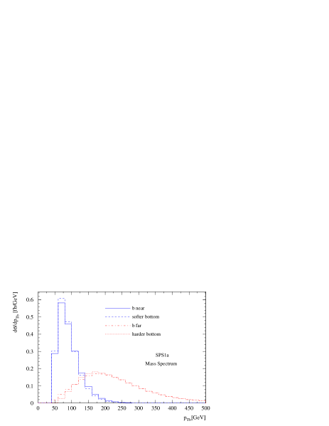
Figure 1: The transverse momentum spectra for the bottom jets in the gluino decay. The tagged bottom jets are ordered according to their appearance (near/far) in the gluon decay chain and according to their transverse momentum.

In some scenarios, like in SPS1a, the mass hierarchy has a favorable impact on the momentum of the jets radiated off the decay cascade. In Fig. 1 we see that just picking the harder of the two bottom jets we can distinguish between ‘near’ (gluino decay) and ‘far’ (sbottom decay) jet on an event–by–event basis, to construct an asymmetry. However, for most of our analysis we choose to ignore this spectrum dependent approach in favor of the general method of distinguishing $b$ and $\bar{b}$ jets by the lepton charge in the $b/\bar{b}$ tag.

The lighter of the two sbottoms and sleptons dominate the long gluino decay chain, but in our numerical analysis we always include all scalar mass eigenstates i.e. we include intermediate $\tilde{b}_{{1,2}}$ as well as $\tilde{\ell}_{{1,2}}$ and $\tilde{\tau}_{{1,2}}$ in the cascade. True off-shell SUSY effects will be strongly suppressed smadgraph . The contribution of the heavier sbottom $\tilde{b}_{{2}}\sim\tilde{b}_{{R}}$ to the gluino decay width is roughly five times smaller than the $\tilde{b}_{{1}}\sim\tilde{b}_{{L}}$ contribution. The leptonic $\tau$ decays we compute in the collinear approximation ($m_{\tau}\ll p_{T,\tau}$).

For the parton–level decay chains we include the UED spectrum in Madgraph madevent and use Smadgraph smadgraph for the SUSY simulation. This way we correctly treat all spin correlations. All final–state momenta are smeared to simulate detector effects. After including a $60\%$ $b$-tagging efficiency, $b$ and $\bar{b}$ can be distinguished by the lepton charge in semileptonic decays ($22\%$ branching ratio times $80\%$ lepton detection efficiency) with a $30\%$ mistag probability btags . When the tagging algorithm yields $bb$ or $\bar{b}\bar{b}$ we discard the events. These detector effects yield an additional $0.11$ dilution factor for the signal.

The gluino signal can be extracted using the basic acceptance cuts:

$$p_{T,b} >50~{}{\rm GeV}\qquad p_{T,\ell} >10~{}{\rm GeV}$$

$$p_{T,j}^{\rm min} >40~{}{\rm GeV} p_{T,j}^{\rm max} >150~{}{\rm GeV}$$

$$|\eta_{i}| <2.4 \Delta R_{ik} >0.4 (i,k=b,j,\ell)$$ (9)

For the associated $\tilde{q}\tilde{g}$ production we require the single jet from the squark decay to pass the $p_{T,j}^{\rm max}$ cut. This selection of cuts leaves us with $10~{}{\rm fb}$ of signal cross section from gluino pairs. To reduce the Standard Model backgrounds we apply the additional rejection cuts:

$$m_{\ell\ell}<80~{}{\rm GeV}\quad M_{\rm eff}>450~{}{\rm GeV}\quad m_{jj}<300~{}{\rm GeV}\$$ (10)

where $M_{\rm eff}=p_{T_{j,1}}+p_{T_{j,2}}+/\!\!\!p_{T}$. After this additional cut our gluino–pair sample is $8.6~{}{\rm fb}$, with a $t\bar{t}jj$ background of $34~{}{\rm fb}$. The associated $\tilde{q}\tilde{g}$ production channel yields a rate ($85~{}{\rm pb}$) about ten times larger than the gluino pair sample while the Standard Model $t\bar{t}j$ background to this channel is $23~{}{\rm fb}$ after cuts, which means that both channels together range around $S/B\sim 1$ skands ; madevent . Our Standard Model and SUSY backgrounds originate from wrongly combined and therefore uncorrelated leptons from independent decays. An efficient way to eliminate these backgrounds beyond the level $S/B\sim 1$ is to subtract the measured opposite flavor dileptons from the same flavor dileptons Gjelsten:2004ki . Because the precise prediction of the remaining small backgrounds is beyond the scope of this paper we will not include SUSY or Standard Model backgrounds in our analysis.

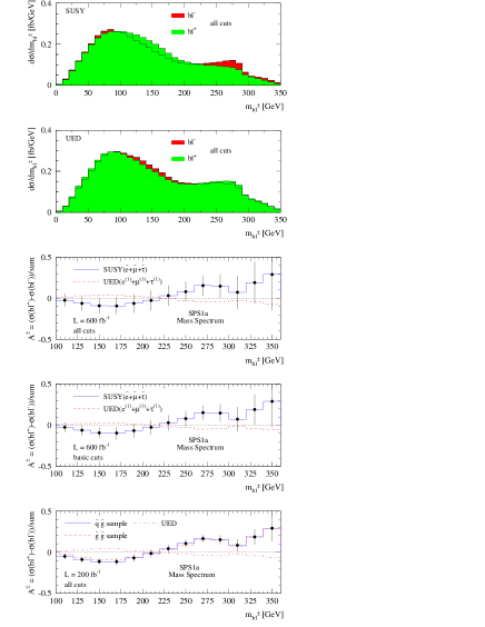
Figure 2: In the first panel we show the $b$–$\ell^{\pm}$ invariant mass distribution after cuts Eqs. (9,10) using only $\tilde{g}\tilde{g}$ production for the parameter point SPS1a. The second panel shows the $m_{b\ell^{\pm}}$ spectrum for the UED interpretation assuming that the first KK states have masses equal to the SUSY particles in the first panel. The third panel contains the asymmetry $A^{\pm}(m_{b\ell})$ defined in Eq. (11) after cuts Eqs. (9,10) and for an integrated luminosity of $600~{}{\rm fb^{-1}}$. The fourth panel is the same, but after basic cuts Eq. (9) only. The last panel shows $A^{\pm}(m_{b\ell})$ using $\tilde{g}\tilde{g}$ and $\tilde{q}\tilde{g}$ production after all cuts and for an integrated luminosity of $200~{}{\rm fb^{-1}}$.

In the two first panels of Fig. 2 we show the distributions for the bottom–lepton invariant masses, both for the SUSY case and for the UED cascade. To avoid using any information but the spin we assume the SPS1a spectrum for the UED particles and normalize their production cross section times branching fractions to the SUSY rate. Because we set the masses equal for the two interpretations (to make the two scenarios indistinguishable in the usual kinematic analysis of edges and thresholds) all additional information in the shape of $m_{b\ell}$ should be equivalent to angular correlations. The two mass distributions are similar, both for the two lepton charges and for the SUSY vs. UED interpretations. Notwithstanding, we can construct a particularly sensitive asymmetry for each of the two interpretations

$$A^{\pm}(m_{b\ell})=\frac{d\sigma/dm_{b\ell^{+}}-d\sigma/dm_{b\ell^{-}}}{d\sigma/dm_{b\ell^{+}}+d\sigma/dm_{b\ell^{-}}}$$ (11)

that is based on possibility of distinguishing $b$ from $\bar{b}$ through their semi-leptonic decays. This asymmetry is equivalent to an asymmetry in $m_{b\ell^{-}}$ vs. $m_{\bar{b}\ell^{-}}$. Moreover, it has the advantage that systematic uncertainties will cancel to a large (yet hard to specify) degree. From the top two panels in Fig. 2 we see that the generally most dangerous systematic error, namely the jet energy scale, will not impact the distinction between a SUSY and an UED interpretations of the gluino cascade decay: shifting the energy on the $x$ axes will, for small $m_{b\ell}$, always enhance the asymmetry for one of the two interpretations and reduce it for the other. We therefore concentrate on the certainly dominant statistical errors in the binned distributions.

The error bars for the asymmetry $A^{\pm}(m_{b\ell})$ shown in the third panel of Fig. 2 correspond to the statistical error per bin, assuming an integrated luminosity of $600~{}{\rm fb^{-1}}$ and taking account only the $\tilde{g}\tilde{g}$ channel. Of course, an optimized measurement of the asymmetry in SUSY and UED scenarios would rely on the shape analysis to optimize the significance, but from Fig. 2 it is obvious that for a hierarchical mass spectrum it is no problem to distinguish a fermionic gluino from a bosonic KK gluon from the (angular) correlations in their decay chains.

In the fourth panel of Fig. 2 we depict the asymmetries after imposing only the acceptance cuts defined in Eq. (9). We confirm that our results are not biased by the harder background–rejection cuts. Finally, the last panel in Fig. 2 shows the individual $\tilde{q}\tilde{g}$ and $\tilde{g}\tilde{g}$ contributions for an integrated luminosity of $200~{}{\rm fb^{-1}}$. Both contributions can indeed be added naively, confirming our claim that these distributions only carry information from angular correlations in the decay kinematics.

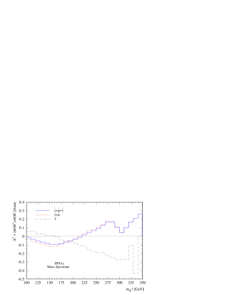
Figure 3: Bottom–lepton asymmetry for the SUSY signal only. The curves shown are for the first and second generation sleptons and for leptons coming from an intermediate $\tilde{\tau}$.

The details of the gluino decay chain reveal an important structure: two leptons in the cascade decay usually come from an intermediate first– or second–generation slepton $\tilde{\ell}_{{1,2}}$, so we can use these leptons to determine the $\tilde{\ell}_{{1,2}}$ masses from kinematical edges. Alternatively, the cascade decay can proceed through a $\tilde{\tau}_{{1,2}}$ with a branching ratio of $6.3\%$ as compared to $0.4\%$ for the first– and second generation sleptons combined. Taking into account the leptonic tau decays the branching fraction from $\tilde{\tau}_{{1,2}}$ drops to $0.2\%$.

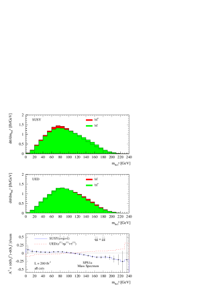
Figure 4: Softer bottom–lepton invariant mass distributions for SUSY (first panel) and UED (second panel) and asymmetry for the SPS1a mass spectrum (last panel), including the $\tau$ contribution. The mass distributions are shown adding the $\tilde{g}\tilde{g}$ and $\tilde{q}\tilde{g}$ contributions after all cuts.

For the parameter point SPS1a the (dominant) lighter selectron or smuon is mostly right handed $\tilde{\ell}_{{1}}\sim\tilde{\ell}_{{R}}$, whereas the lighter stau is mostly left handed $\tilde{\tau}_{{1}}\sim\tilde{\tau}_{{L}}$ due to the renormalization group running and the fairly large $\tan\beta=10$. This means the contribution of the stau to the mass asymmetry is opposite to the selectron and smuon contributions. In Fig. 3 we see how the $\tilde{\tau}_{{1}}$ can in principle wash out the asymmetry from selectrons and smuons. Luckily, the impact of the $\tilde{\tau}$ on our asymmetry given in Eq. (11) is small because leptons from tau decays are softer and hence less likely pass the cuts. After cuts the contribution from staus is about five times smaller than the combined selectron and smuon signal. We will further discuss the different pattern for intermediate left and right handed sleptons as a general feature for the gluino cascade in Sec. .6.

As mentioned above, the SUSY spectrum might be such that it is possible to identify the (near) bottom jet from the gluino decay since it is softer. In those cases where we can identify the softer $b$ jet with the near $b$ jet for each event a similar asymmetry can be defined as

$$A^{\pm}(m_{b_{s}\ell})=\frac{d\sigma/dm_{b_{s}\ell^{+}}-d\sigma/dm_{b_{s}\ell^{-}}}{d\sigma/dm_{b_{s}\ell^{+}}+d\sigma/dm_{b_{s}\ell^{-}}}$$ (12)

Note that here the symbol $b$ means either $b$ or $\bar{b}$, without distinction. Fig. 4 shows that $A^{\pm}(m_{b_{s}\ell})$ can be an efficient tool to discriminate between SUSY and UED decay cascades for a hierarchical mass spectrum.

.4 Purely Hadronic Correlations

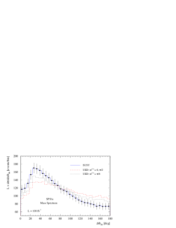
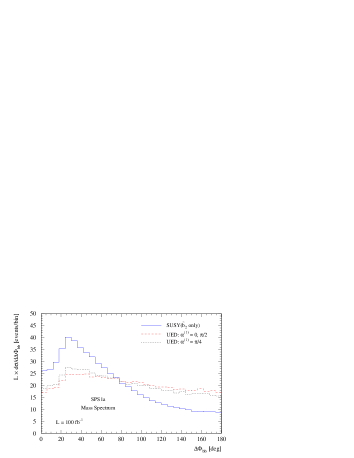
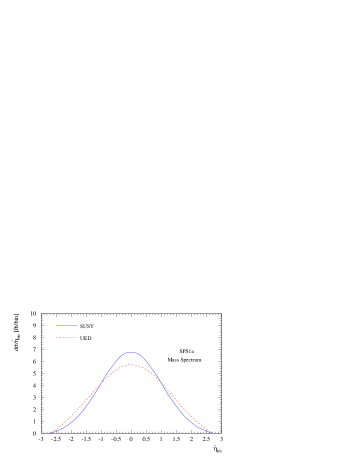
Figure 5: From the top: (i) azimuthal angle between the two bottom jets for UED and SUSY decay chains including $\tilde{b}_{{1}}$ and $\tilde{b}_{{2}}$; (ii) including only the effect of $\tilde{b}_{{2}}$ exchange; (iii) averaged bottom jet rapidities. In all cases we assume the SPS1a spectrum and add the rates for $\tilde{g}\tilde{g}$ and $\tilde{q}\tilde{g}$ production.

The correlation between a lepton and a bottom jet is only one of the distributions we can use to distinguish the two interpretations of the decay cascade. Unfortunately, it has been shown for squark decays that purely leptonic distributions are not as useful as mixed lepton–jet correlations smillie . However, in the gluino decay chain there is an additional jet, so we can build purely hadronic correlations. This has the advantage of being independent of the $\tilde{\chi}^{0}_{{2}}$ decay, which can involve not only intermediate sleptons, but also intermediate gauge bosons or even three-body decay kinematics.

In general, we expect all spin information to be hidden in angular correlations. After exploiting the kinematic endpoints to measure the masses in the cascade decays, we use the shape of invariant mass distributions as a Lorentz–invariant formulation of the angles. The only well defined angles we can observe at the LHC are azimuthal angles between for example the two bottom jets, because they are invariant under boosts in the beam direction. In Fig. 5 we present the distribution $d\sigma/d\Delta\phi_{bb}$, which exhibits a distinct behavior for SUSY and UED decay chains. These two possibilities can be disentangled through the asymmetry:

$$\frac{\sigma(\Delta\Phi_{bb}<90^{o})-\sigma(\Delta\Phi_{bb}>90^{o})}{\sigma(\Delta\Phi_{bb}<90^{o})+\sigma(\Delta\Phi_{bb}>90^{o})}$$ (13)

This asymmetry assumes small values $0.08\pm 0.02$ for the UED spin assignment with the usual mass–suppressed mixing angle $\alpha^{(1)}\sim 0$. On the other hand, for the SUSY interpretation it is significantly larger $0.24\pm 0.02$. The quoted errors are statistical errors for the combination of the gluino–pair and associated gluino–squark production channels and an integrated luminosity of $100~{}{\rm fb^{-1}}$. The UED cross section is as usually normalized to the SUSY rate.

To estimate the dependence of the $\Delta\Phi_{bb}$ distribution on the couplings of the sbottom we present this distribution for a purely $\tilde{b}_{{2}}$ decay chain in the second panel of Fig. 5. Indeed, $\Delta\Phi_{bb}$ is insensitive to the left–right couplings of bottom jets to the intermediate SUSY particles which makes it a robust discriminating observable for spin correlations. This reflects the scalar nature of the intermediate sbottom. As a matter of fact, in analogy with the purely leptonic correlation smillie we find that the different UED and SUSY behavior shown in Fig. 5 is mostly due to the boost of the heavy gluino or KK gluon.

According to Sec. .2 there is not very much room to modify the UED Lagrangian to bring kinematical correlations closer to the SUSY prediction. The KK weak mixing angle $\theta_{w}^{(n)}$ in Eq. (5) is fixed by the interaction eigenstates’ masses, so we can not change it while keeping the masses fixed. The coupling structure in the decay matrix element is of the general kind $(L^{2}+R^{2})$, as long as the KK singlet and doublet fermions are close in mass. The same limitations hold when we try to adjust the mixing between the singlet and doublet KK fermions, described by the angle $\alpha^{(n)}$, Eq. (2). In contrast to the 3rd–generation sfermion sector in the MSSM, the UED mixing angle is not a (third) free parameter, even if we move around the masses invoking boundary conditions. Nevertheless, for illustration purpose we vary $\alpha^{(n)}$ in Fig. 5 to check whether the SUSY $\Delta\Phi_{bb}$ can be reproduced by a UED decay chain with different couplings to the fermions. From the two top panels of Fig. 5 we see that the changes in the UED distribution are not sufficient to mimic the SUSY predictions.

Our final observable is the average bottom rapidity Meade:2006dw $\bar{\eta}_{bb}=(\eta_{b}+\eta_{\bar{b}})/2$ which we show in the bottom panel of Fig. 5. As we can see the bottom jets from gluino cascades are typically more central than those from the KK–gluon cascades, however, it is difficult to discriminate the SUSY curve from UED on a bin-by-bin basis. Therefore, we define another asymmetry

$$\frac{\sigma(|\bar{\eta}_{bb}|<1.0)-\sigma(|\bar{\eta}_{bb}|>1.0)}{\sigma(|\bar{\eta}_{bb}|<1.0)+\sigma(|\bar{\eta}_{bb}|>1.0)}\;\;,$$ (14)

which gives $0.40\pm 0.02$ for SUSY and $0.24\pm 0.02$ for UED. These results were obtained using the $\tilde{q}\tilde{g}$ and $\tilde{g}\tilde{g}$ production channels and an integrated luminosity of $100~{}{\rm fb^{-1}}$. As always, we normalize the UED signal to the SUSY rate.

.5 Degenerate UED-type Spectrum

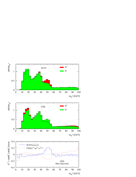
Figure 6: Bottom–lepton invariant mass distributions for SUSY (first panel) and UED (second panel) and asymmetry (third panel), in arbitrary units, for gluino pair production and after the background rejection cuts Eq. (10), for the UED mass spectrum described in Sec. .2.

In the analysis above we have made a crucial assumptions: a hierarchical spectrum of the new particles responsible for the cascade decay. In UED, the first KK excitations will tend to be mass degenerate, unless this degeneracy is broken by boundary conditions for the different fields or by large loop corrections. For the highly degenerate spectrum listed in Sec. .2 the outgoing fermions become very soft and the cross section after cuts decreases, which translates into a strongly reduced precision of our measurements. Moreover, the invariant mass distributions shown in Fig. 6 lose their characteristic pattern, for the SUSY as well as for the UED prediction smillie and their associated asymmetries are indistinguishable within the expected statistical errors. The same is unfortunately true for the angular distributions of the $b$ jets. The hard cuts imposed to separate the signal from $t\bar{t}$+jets backgrounds determine completely the shape of angular distributions and invariant masses in both descriptions.

.6 Left and Right Sleptons and Squarks

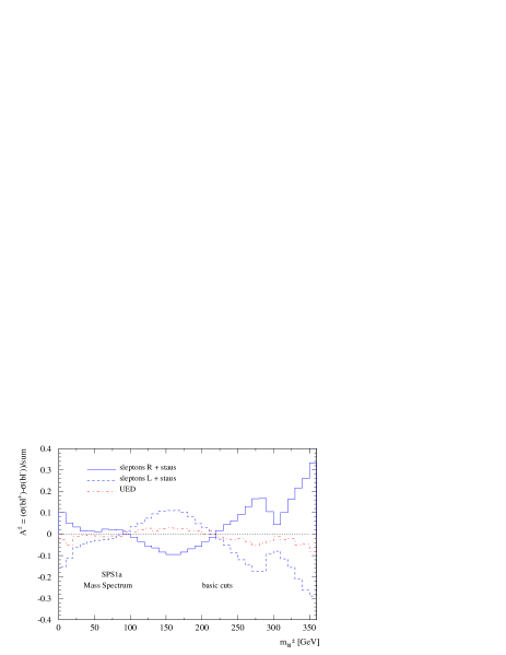
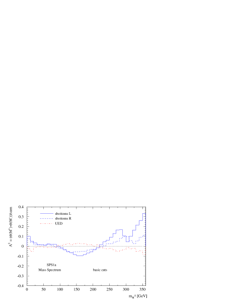
Figure 7: Asymmetry for an SPS1a mass spectrum and a supersymmetric gluino cascade, but varying the coupling of the cascade spectrum between purely left handed and purely right handed.

As we point out in Sec. .3 the left handed and right handed coupling of the slepton in the cascade is crucial to determine the asymmetry in the lepton–bottom invariant mass. Or (in other words), the same distributions we use to determine the spin of the cascade we can use to determine the nature of the squark and slepton appearing in the cascade. This twofold ambiguity is the major source of degeneracies in the determination of the MSSM mass parameters at the LHC sfitter ; gordi , and it can be broken by the shape of $m_{b\ell}$ or by the variables $\Delta\phi_{b\bar{b}}$ and $\bar{\eta}_{b\bar{b}}$.

In the MSSM we are free to assign the two left and right soft–breaking masses. For partners of essentially massless Standard Model particles the mass eigenstates and the interaction eigenstates are identical. As mentioned above, the light–flavor sleptons in the SPS1a parameter point are of the kind $\tilde{\ell}_{{1,2}}\sim\tilde{\ell}_{{R,L}}$, the staus couple like $\tilde{\tau}_{{1,2}}\sim\tilde{\tau}_{{L,R}}$, and the sbottoms like $\tilde{b}_{{1,2}}\sim\tilde{b}_{{L,R}}$. If we assume we know the nature of the two lightest neutralinos we can roughly determine the nature of a decaying squark from its branching fractions $\tilde{q}\to q\tilde{\chi}^{0}_{{1}}$ and $\tilde{q}\to q\tilde{\chi}^{0}_{{2}}\to q\ell^{+}\ell^{-}\tilde{\chi}^{0}_{{1}}$, because the bino and the wino fraction in the neutralino couple differently to left and right sfermions.

For the sleptons we usually cannot access branching fractions at the LHC because we cannot rely on a direct production channel. For example if the mass hierarchy is SPS1a-like ($m_{\tilde{\ell}_{\scriptscriptstyle{2}}}>m_{\tilde{\chi}^{\scriptscriptstyle 0}_{\scriptscriptstyle{2}}}>m_{\tilde{\ell}_{\scriptscriptstyle{1}}}$) squark and gluino cascade decays are the only source of information on sleptons. They are dominated by the lighter of the sleptons which is produced on–shell in the cascade decay. In that situation we can determine the chiral structure of the slepton couplings from the same distributions we use to distinguish a gluino cascade from a KK gluon cascade. For the squark cascade this feature has been discussed independent of the spin measurement sleptons . We illustrate the link between slepton couplings and spins in the top panel of Fig. 7 where we display the asymmetry as a function of $m_{b\ell^{\pm}}$ for left and right handed sleptons. The asymmetry shows the opposite behavior for $\ell_{R}$ and $\ell_{L}$ and consequently can be used as an indication of the $\tilde{\ell}_{{1,2}}\sim\tilde{\ell}_{{R,L}}$ assignment. For scalar taus, Fig. 3 shows that the same measurement is possible, provided we identify the tau leptons from the cascade reliably tautag . On the other hand the $\tilde{b}_{{R}}$ and $\tilde{b}_{{L}}$ contributions to the asymmetry are very similar, as we can see in the bottom panel of Fig. 7, so from these distributions we cannot distinguish the two bottom states.

.7 Outlook

Proving the presence of a Majorana gluino is the prime task for the LHC to show that new TeV–scale physics is supersymmetric. It has been known for a long time that like–sign dileptons are a clear sign for the Majorana nature of a newly found strongly interacting particle likesign . The remaining loop hole in this argument is to show that the gluino candidate is actually a fermion. Recently, it has been shown how to distinguish supersymmetric partners of Standard Model particles from same-spin partners, for example described by UED models barr ; smillie .

We extend these spin analyses to the case of a gluino decaying through the bottom cascade. This is the decay chain which can best be used for the gluino mass measurement mgl . The decay cascade can be interpreted as a SUSY or as a UED signal, with identical particle masses. To distinguish the two spin patterns it is crucial to limit the observables to angular correlations linked to the spins and to ignore additional information which can come from production cross sections times branching rations or from ‘typical’ mass spectra.

Using a list of asymmetries (constructed from lepton–bottom correlations or from pure bottom–bottom correlations) we distinguish between the SUSY and the UED cascade interpretations and thus determine the spin of the gluino. The spin information which is clearly present in the decay kinematics is always entangled with the left and right handed sfermion couplings sleptons . Turning the argument around, we find that the slepton coupling structure can be determined from these kinds of correlations together with the spins. This reduces possible degeneracies in the SUSY parameter extraction sfitter ; gordi .

While spin analyses for SUSY models (using UED as a straw man) are an exciting new development for the LHC, they are much more complex than ILC spin analyses tesla because of the entanglement with the left and right handed couplings of supersymmetric scalars. On the other hand, the gluino will likely not be pair produced at the ILC. For example, to test gaugino masses unification we need the gluino spin measurement at the LHC to unambiguously identify the three gauginos and evolve their masses to some high scale sfitter ; pmz_unification .

- (1) For reviews of SUSY, see e.g. : I. J. R. Aitchison, hep-ph/0505105; S. P. Martin, hep-ph/9709356.
- (2) S. Dawson, E. Eichten and C. Quigg, Phys. Rev. D 31, 1581 (1985).
- (3) W. Beenakker, R. Höpker, M. Spira and P. M. Zerwas, Nucl. Phys. B 492, 51 (1997); T. Plehn, arXiv:hep-ph/9809319; W. Beenakker, M. Krämer, T. Plehn, M. Spira and P. M. Zerwas, Nucl. Phys. B 515, 3 (1998); W. Beenakker, M. Klasen, M. Krämer, T. Plehn, M. Spira and P. M. Zerwas, Phys. Rev. Lett. 83, 3780 (1999); Propspino2.0 publicly available from www.ph.ed.ac.uk/~tplehn
- (4) R. M. Barnett, J. F. Gunion and H. E. Haber, in in Proc. of the Summer Study on High–Energy Physics in the 1990s, Snowmass 1988, ed. S. Jensen; H. Baer, X. Tata and J. Woodside, ibid; H. Baer, X. Tata and J. Woodside, Phys. Rev. D 41, 906 (1990); R. M. Barnett, J. F. Gunion and H. E. Haber, Phys. Lett. B 315, 349 (1993); V. Barger, W.-Y. Keung and R. J. N. Phillips, Phys. Rev. Lett. 55, 166 (1985).
- (5) S. Kraml and A. R. Raklev, arXiv:hep-ph/0512284; C. Balazs, M. Carena and C. E. M. Wagner, Phys. Rev. D 70, 015007 (2004).
- (6) W. Beenakker, R. Höpker, T. Plehn and P. M. Zerwas, Z. Phys. C 75, 349 (1997); J. Hisano, K. Kawagoe and M. M. Nojiri, Phys. Rev. D 68, 035007 (2003); M. Mühlleitner, A. Djouadi and Y. Mambrini, Comput. Phys. Commun. 168, 46 (2005).
- (7) T. Appelquist, H. C. Cheng and B. A. Dobrescu, Phys. Rev. D 64, 035002 (2001); T. G. Rizzo, Phys. Rev. D 64, 095010 (2001); D. A. Dicus, C. D. McMullen and S. Nandi, Phys. Rev. D 65, 076007 (2002); C. Macesanu, arXiv:hep-ph/0510418; G. Burdman, B. A. Dobrescu and E. Ponton, arXiv:hep-ph/0601186; M. Battaglia, A. Datta, A. De Roeck, K. Kong and K. T. Matchev, JHEP 0507, 033 (2005); M. Battaglia, A. K. Datta, A. De Roeck, K. Kong and K. T. Matchev, arXiv:hep-ph/0507284.
- (8) H. C. Cheng, K. T. Matchev and M. Schmaltz, Phys. Rev. D 66, 056006 (2002); A. Datta, K. Kong and K. T. Matchev, Phys. Rev. D 72, 096006 (2005) [Erratum-ibid. D 72, 119901 (2005)]; A. Datta, G. L. Kane and M. Toharia, arXiv:hep-ph/0510204.
- (9) H. Bachacou, I. Hinchliffe and F. E. Paige, Phys. Rev. D 62, 015009 (2000); B. C. Allanach, C. G. Lester, M. A. Parker and B. R. Webber, JHEP 0009, 004 (2000); C. G. Lester, M. A. Parker and M. J. White, JHEP 0601, 080 (2006). C. G. Lester, arXiv:hep-ph/0603171.
- (10) B. K. Gjelsten, D. J. Miller and P. Osland, JHEP 0412, 003 (2004); B. K. Gjelsten, D. J. Miller and P. Osland, JHEP 0506, 015 (2005).
- (11) A. J. Barr, Phys. Lett. B 596, 205 (2004); A. J. Barr, JHEP 0602, 042 (2006).
- (12) J. M. Smillie and B. R. Webber, JHEP 0510, 069 (2005).
- (13) P. Meade and M. Reece, arXiv:hep-ph/0601124.
- (14) R. Lafaye, T. Plehn and D. Zerwas, arXiv:hep-ph/0404282 and arXiv:hep-ph/0512028; P. Bechtle, K. Desch and P. Wienemann, arXiv:hep-ph/0412012.
- (15) N. Arkani-Hamed, G. L. Kane, J. Thaler and L. T. Wang, arXiv:hep-ph/0512190.
- (16) B. C. Allanach et al., Eur. Phys. J. C 25, 113 (2002).
- (17) E. Accomando et al. [ECFA/DESY LC Physics Working Group Collaboration], Phys. Rept. 299, 1 (1998); J. A. Aguilar-Saavedra et al. [ECFA/DESY LC Physics Working Group arXiv:hep-ph/0106315; J. A. Aguilar-Saavedra et al., arXiv:hep-ph/0511344.
- (18) T. Bringmann, Cosmological Aspects of Universal Extra Dimensions, PhD Thesis.
- (19) K. Hagiwara et al., Phys. Rev. D 73, 055005 (2006); G. C. Cho, K. Hagiwara, J. Kanzaki, T. Plehn, D. Rainwater and T. Stelzer, Phys. Rev. D 73, 054002 (2006).
- (20) T. Stelzer, F. Long, Comput. Phys. Commun. 81 (1994) 357; F. Maltoni and T. Stelzer, JHEP 0302, 027 (2003).
- (21) ATLAS detector and physics performance, Technical Design Report, section 17.2.2.4; R. Hawkings, Eur. Phys. J. C 34, s109-s116 (2004).
- (22) T. Plehn, D. Rainwater and P. Skands, arXiv:hep-ph/0510144.
- (23) B. K. Gjelsten, D. J. Miller and P. Osland, JHEP 0412, 003 (2004).
- (24) T. Goto, K. Kawagoe and M. M. Nojiri, Phys. Rev. D 70, 075016 (2004) [Erratum-ibid. D 71, 059902 (2005)].
- (25) F. Tarrade, LAPP-EXP 2005-13 (2005).
- (26) G. A. Blair, W. Porod and P. M. Zerwas, Phys. Rev. D 63, 017703 (2001).