Plasma Instabilities in an Anisotropically Expanding Geometry

Abstract

We study (3+1)D kinetic (Boltzmann-Vlasov) equations for relativistic plasma particles in a one-dimensionally expanding geometry (a special Kasner-type universe) motivated by ultrarelativistic heavy-ion collisions. We set up local equations in terms of Yang-Mills potentials and auxiliary fields that allow simulations of hard-(expanding)-loop (HEL) dynamics on a lattice. We determine numerically the evolution of plasma instabilities in the linear (Abelian) regime and also derive their late-time behavior analytically, which is consistent with recent numerical results on the evolution of the so-called melting color-glass condensate. We also find a significant delay in the onset of growth of plasma instabilities which are triggered by small rapidity fluctuations, even when the initial state is highly anisotropic.

Plasma instabilities have recently been suggested to play a major role in the equilibration of matter created by an ultrarelativistic heavy-ion collision, e.g. at the Relativistic Heavy Ion Collider (RHIC) or the Large Hadron Collider (LHC) Randrup:2003cw ; Romatschke:2003ms ; Arnold:2003rq ; Rebhan:2004ur ; Dumitru:2005gp ; Arnold:2005vb . Shortly after such a collision, saturation scenarios McLerran:1993ni ; Iancu:2003xm indicate that the typical momentum of a particle in the local plasma rest frame is much larger transverse to the collision axis than parallel to it. This momentum anisotropy inevitably leads to a so-called Weibel Weibel:1959 (or filamentation) plasma instability that manifests itself by rapidly growing transverse magnetic fields. If large enough, a transverse magnetic field bends the trajectories of particles out of the transverse plane, thus making the system more isotropic. Plasma instabilities are therefore a prime candidate for causing rapid isotropization of a quark-gluon plasma, especially since they act on a time-scale that is parametrically shorter than that of scatterings by at least one power of the strong coupling constant $g$.

There are, however, some caveats: for instance, numerical simulations Rebhan:2004ur ; Arnold:2005vb of non-Abelian Yang-Mills equations in the (stationary) hard-loop approximation Mrowczynski:2004kv have shown that the initially exponential growth of gauge fields slows down to a weak linear growth when self-interactions of the unstable modes become important and energy in unstable modes cascades to stable modes of higher momentum Arnold:2005ef . Interestingly, this may lead to the generation of anomalously low viscosity Asakawa:2006tc .

Maybe more importantly, the matter created in a heavy-ion collision is believed to escape relatively unimpeded in the longitudinal direction (the direction of the collision axis). This effectively one-dimensional expansion decreases the density of hard particles Mueller:1999pi ; Baier:2002bt and thus attenuates the growth rate of plasma instabilities. On the other hand, the expansion increases the degree of anisotropy, thus making more and more higher-momentum modes unstable. While numerical simulations of classical Yang-Mills dynamics have provided some qualitative understanding of the counterplay of plasma instabilities and expansion Romatschke:2005pm , an analysis based on the hard-loop approximation is desirable, in particular to address systematically the fate of non-Abelian plasma instabilities and of the associated energy cascade. The purpose of this Letter is to develop the basis for such a treatment. We generalize the anisotropic hard-loop effective theory of Refs. Rebhan:2004ur ; Arnold:2005vb to the case of a dynamical, boost-invariantly expanding background, thus preparing the ground for corresponding lattice simulations. We work out explicitly the already rather nontrivial dynamics in the linear (Abelian) regime (which thus are in principle of interest also to ultrarelativistic conventional plasma physics) and discuss possible implications for ultrarelativistic heavy-ion collisions.

Ignoring the effects of collisions, the dynamics of collective modes in a non-Abelian plasma is determined by the gauge covariant Boltzmann-Vlasov equations

$$p\cdot D\,\delta f_{a}(\mathbf{p},\mathbf{x},t)=gp_{\mu}F^{\mu\nu}_{a}\partial^{(p)}_{\nu}f_{0}(\mathbf{p},\mathbf{x},t),$$ (1)

coupled to the Yang-Mills equations

$$D_{\mu}F^{\mu\nu}_{a}=j^{\nu}_{a}=g\int{d^{3}p\over(2\pi)^{3}}\frac{p^{\mu}}{2p^{0}}\delta f_{a}(\mathbf{p},\mathbf{x},t).$$ (2)

Here $F^{\mu\nu}_{a}=\partial^{\mu}A^{\nu}_{a}-\partial^{\nu}A^{\mu}_{a}+gf_{abc}A^{\mu}_{b}A^{\nu}_{c}$ is the field strength tensor in the adjoint representation, $D^{\mu}_{ac}=\delta_{ac}\partial^{\mu}+gf_{abc}A^{\mu}_{b}$ is the gauge-covariant derivative, $A^{\mu}$ is the gauge-potential. $f_{0}(\mathbf{p},\mathbf{x},t)$ is the (suitably normalized) color-neutral background distribution of hard particles and $\delta f_{a}(\mathbf{p},\mathbf{x},t)$ its colored fluctuations. Eq.(1) requires that the background $f_{0}$ satisfies $p\cdot\partial\,f_{0}(\mathbf{p},\mathbf{x},t)=0$ (which is trivially fulfilled when $f_{0}$ is space-time independent). Assuming that the matter created after a heavy-ion collision expands longitudinally in a boost-invariant way and is sufficiently large in the transverse direction such that transverse gradients are small, we take

$$f_{0}(\mathbf{p},x)=f_{0}(p_{\perp},p^{z},z,t)=f_{0}(p_{\perp},tp^{z}-zp^{0})$$ (3)

which also satisfies $p\cdot\partial\,f_{0}(\mathbf{p},\mathbf{x},t)=0$.

To describe the dynamics of fluctuations around a boost-invariant background, convenient coordinates are proper time $\tau=\sqrt{t^{2}-z^{2}}$ and space-time rapidity $\eta={\rm arctanh}\frac{z}{t}$. The metric in these coordinates is $g_{\tau\tau}{\rm=1}$, $g_{ij}{\rm=-}\delta_{ij}{\rm}$, $g_{\eta\eta}{\rm=-}\tau^{2}$, $i{\rm=}1,2$, thus corresponding to a one-dimensionally expanding space-time geometry.

Transforming the set of equations (1,2) to the coordinates $x^{\alpha}=(\tau,x^{i},\eta)$ (denoted collectively by Greek letters from the beginning of the alphabet) we find

$$p\cdot D\,\delta f^{a}|_{p^{\mu}} = gp^{\alpha}F_{\alpha\beta}^{a}\partial_{(p)}^{\beta}f_{0}(\mathbf{p}_{\perp},p_{\eta}),$$ (4)

$${1\over\tau}D_{\alpha}\left(\tau F^{\alpha\beta}\right) = j^{\beta}=\frac{g}{2}\int{d^{2}p_{\perp}dy\over(2\pi)^{3}}p^{\beta}\delta f\,,$$ (5)

where the derivative of $\delta f^{a}$ has to be taken at fixed $p^{\mu}$ as opposed to fixed $p^{\alpha}$. Here we have introduced also momentum rapidity $y={\rm atanh}(p^{0}/p^{z})$, such that $p^{\tau}=|{\bf p^{\perp}}|\cosh{(y-\eta)}$, $p^{\eta}=|{\bf p^{\perp}}|\tau^{-1}\sinh{(y-\eta)}$.

We assume that at the hypersurface $\tau=\tau_{\rm iso}$ the background $f_{0}$ is isotropic and choose the specific model

$$f_{0}(\mathbf{p},x)=f_{\rm iso}\left(\sqrt{p_{\perp}^{2}+p_{\eta}^{2}/\tau_{\rm iso}^{2}}\right),$$ (6)

which corresponds to increasingly oblate momentum space anisotropy at $\tau>\tau_{\rm iso}$ (but prolate anisotropy for $\tau<\tau_{\rm iso}$). However, in what follows we shall start the time evolution at nonzero proper time $\tau_{0}$, allowing for the fact that a plasma description will not make sense at arbitrarily small times, and we shall mostly consider the situation that the initial momentum distribution is highly oblate at $\tau_{0}$, i.e. $\tau_{0}\gg\tau_{\rm iso}$. The distribution function $f_{0}$ has the same form as the one used in Refs. Romatschke:2003ms ; Rebhan:2004ur , but the anisotropy parameter $\xi$ therein is now space-time dependent according to $\xi(\tau)=(\tau/\tau_{\rm iso})^{2}-1.$

Since $p\cdot\partial\,[\partial_{(p)}^{\alpha}f_{0}(\mathbf{p}_{\perp},p_{\eta})]=0$, we can solve Eq. (4) by introducing auxiliary fields $W^{a}_{\alpha}(\tau,x^{i},\eta;v^{i},y)$ in

$$\delta f^{a}(x;p)=-gW^{a}_{\alpha}(\tau,x^{i},\eta;v^{i},y)\partial_{(p)}^{\alpha}f_{0}(p_{\perp},p_{\eta})$$ (7)

that obey

$$v\cdot D\,W_{\alpha}(\tau,x^{i},\eta;v^{i},y)=v^{\beta}F_{\alpha\beta},$$ (8)

where $v^{\alpha}\equiv{p^{\alpha}\over|{\mathbf{p}_{\perp}}|}=(\cosh(y-\eta),\cos\phi,\sin\phi,\frac{\sinh(y-\eta)}{\tau}).$ At any given space-time point the fields $W_{\alpha}$ depend only on the velocity of the hard particles and not on their momentum scale, and thus directly generalize the auxiliary fields $W_{\mu}(x;\mathbf{v})$ of the hard-loop formalism in a static background distribution $f_{0}$ Blaizot:2001nr ; Mrowczynski:2004kv .

For $f_{0}$ of Eq.(6), the induced current $j^{\beta}$ takes the form

$$j^{\alpha}\!=\!-{m_{D}^{2}\over 2}\int_{0}^{2\pi}{d\phi\over 2\pi}\int\frac{dy\ v^{\alpha}}{\left(1+{v_{\eta}^{2}\over\tau_{\rm iso}^{2}}\right)^{2}}\left\{v^{j}W_{j}-{v_{\eta}\over\tau_{\rm iso}^{2}}W_{\eta}\right\}\,,$$ (9)

where $m^{2}_{D}=-g^{2}\int_{0}^{\infty}{dp\,p^{2}\over(2\pi)^{2}}f^{\prime}_{\rm iso}(p)$ is the Debye mass of the isotropic case. A short calculation confirms that the current is covariantly conserved, $D_{\alpha}\tau j^{\alpha}=0$.

The Eqs. (8), (9) together with the Yang-Mills equations (5) can be simulated on a 3-dimensional lattice by discretizing space-time and introducing lattice links in a standard way Krasnitz:1998ns and by also discretizing the residual momentum variables $\phi$ and $y$ in order to have a finite number of $W$ fields. This directly generalizes the discretized hard-loop effective equations of motions of Ref.Rebhan:2004ur to what may be called the hard-expanding-loop (HEL) case. As in the stationary case, momentum discretizations that respect reflection invariance (now with respect to $\phi$ and $y-\eta$) automatically ensure covariant current conservation, $D_{\alpha}\tau j^{\alpha}=0$.

In this Letter, we initiate this program by studying the onset of plasma instabilities and their evolution in the linear regime, where their non-Abelian self-interactions are still negligible and where we can avoid a discretization of $\phi$ and $y$ by solving the equations of motions of the auxiliary fields $W_{\alpha}(\tau,x^{i},\eta;\phi,y)$. In a stationary plasma with oblate momentum-space anisotropy, the most unstable modes have wave vectors along the longitudinal direction. A particularly interesting case can thus be studied by neglecting the transverse dynamics ($\partial_{i}A^{\alpha}=0$). Linearizing in the gauge potentials we have

$$\left[\tau^{-1}\partial_{\tau}\tau\partial_{\tau}-\tau^{-2}\partial_{\eta}^{2}\right]A^{i}(\tau,\eta)=j^{i},\quad\tau\partial_{\tau}\tau^{-1}\partial_{\tau}A_{\eta}=j_{\eta},$$ (10)

in the gauge $A^{\tau}=0$. Eq. (8) can be solved by the method of characteristics which gives

$$W_{\alpha}(\tau,\eta;\phi,y) = \int_{\tau_{0}}^{\tau}d\tau^{\prime}\frac{\left.v^{\beta}F_{\alpha\beta}\right|_{\tau^{\prime},\eta(\tau^{\prime})}}{\cosh(y-\eta(\tau^{\prime}))}\,,$$

$$y-\eta(\tau^{\prime}) = {\rm asinh}{\left(\frac{\tau}{\tau^{\prime}}\sinh{(y-\eta)}\right)},$$ (11)

where $\eta{(\tau^{\prime})}$ is the solution along the characteristic. Within our approximation we can thus proceed to evaluate the $d\phi$ integral in Eq.(9), finding

$$j^{i}\! = \!-\frac{m_{D}^{2}}{4}\,\int_{-\infty}^{\infty}dy\,\left(1+{v_{\eta}^{2}\over\tau_{\rm iso}^{2}}\right)^{-2}\int^{\tau}_{\tau_{0}}d\tau^{\prime}$$

$$\!\!\!\!\!\!\!\!\!\!\!\!\times\left[\left(\partial_{\tau}^{\prime}-\frac{\tanh{\bar{\eta}^{\prime}}}{\tau^{\prime}}\partial_{\eta^{\prime}}\right)A^{i}(\tau^{\prime},\eta^{\prime})+{v_{\eta}\over\tau_{\rm iso}^{2}}\,\frac{\partial_{\eta^{\prime}}A^{i}(\tau^{\prime},\eta^{\prime})}{\cosh\bar{\eta}^{\prime}}\right],$$

$$j^{\eta}\!\! = \!\!-{m_{D}^{2}\over 2\tau_{\rm iso}^{2}}\int\frac{dy\,v^{\eta}v_{\eta}}{\left(1+{v_{\eta}^{2}\over\tau_{\rm iso}^{2}}\right)^{2}}\int^{\tau}_{\tau_{0}}d\tau^{\prime}\partial_{\tau^{\prime}}A_{\eta}(\tau^{\prime},\eta^{\prime}),$$ (12)

where $\eta^{\prime}=\eta(\tau^{\prime})$ and $\bar{\eta}^{\prime}=\eta(\tau^{\prime})-y$.

Introducing a Fourier transform in space-time rapidity,

$$A^{i}(\tau,\eta)=\int\frac{d\nu}{2\pi}\exp(i\nu\eta)\widetilde{A}^{i}(\tau,\nu),$$ (13)

and choosing $A^{\mu}(\tau_{0})=0$ for simplicity, we find

$$\widetilde{j}^{i}(\tau,\nu)=-\frac{m_{D}^{2}}{4}\int\frac{dy}{\left(1+{\tau^{2}\sinh^{2}{y}\over\tau_{\rm iso}^{2}}\right)^{2}}\biggl{\{}\widetilde{A}^{i}(\tau,\nu)$$

$$\quad-\int_{\tau_{0}}^{\tau}d\tau^{\prime}\frac{\widetilde{A}^{i}(\tau^{\prime},\nu)\tau^{\prime 2}}{\tau_{\rm iso}^{2}}\partial_{\tau^{\prime}}e^{i\nu\left[y-{\rm asinh}{\left(\frac{\tau}{\tau^{\prime}}\sinh{y}\right)}\right]}\biggr{\}},$$

$$\widetilde{j}^{\eta}(\tau,\nu)={m_{D}^{2}\over 2\tau_{\rm iso}^{2}}\int\frac{dy\,\sinh^{2}{y}}{\left(1+{\tau^{2}\sinh^{2}{y}\over\tau_{\rm iso}^{2}}\right)^{2}}\biggl{\{}\widetilde{A}_{\eta}(\tau,\nu)$$

$$\quad-\int_{\tau_{0}}^{\tau}d\tau^{\prime}\widetilde{A}_{\eta}(\tau^{\prime},\nu)\partial_{\tau^{\prime}}e^{i\nu\left[y-{\rm asinh}{\left(\frac{\tau}{\tau^{\prime}}\sinh{y}\right)}\right]}\biggr{\}}.\qquad$$ (14)

Below we solve the integro-differential Eqs. (10), (14) numerically. The late time behavior $\tau\gg\tau_{0}$, however, may be studied analytically by expanding $\exp{\left[i\nu\left(y-{\rm asinh}{\left(\frac{\tau}{\tau^{\prime}}\sinh{y}\right)}\right)\right]}$ in Eq.(14) around $\tau^{\prime}=\tau$ and subsequently acting with $\partial_{\tau}^{2}\tau^{2}$ on Eqs.(10). In this limit, the integro-differential equations turn into ordinary differential equations for each mode $\nu$,

$$\left[\partial_{\tau}^{2}\tau\partial_{\tau}\tau\partial_{\tau}+\nu^{2}\partial_{\tau}^{2}+\mu\partial_{\tau}^{2}\tau-\mu\nu^{2}{\tau^{-1}}\right]\widetilde{A}^{i}(\tau,\nu)\simeq 0,$$ (15)

$$\left[\partial_{\tau}{\tau^{-1}}\partial_{\tau}+2\mu{\tau^{-2}}\right]\widetilde{A}_{\eta}(\tau,\nu)\simeq 0,$$ (16)

where $\mu={1\over 8}{m_{D}^{2}\pi\tau_{\rm iso}}$. From Eq. (16) we find for the late-time behavior of longitudinal fields $A_{z}=\tau^{-1}A_{\eta}\cosh\eta$

$$\tau^{-1}\widetilde{A}_{\eta}(\tau,\nu)\simeq c_{1}J_{2}\left(2\sqrt{2\mu\tau}\right)+c_{2}Y_{2}\left(2\sqrt{2\mu\tau}\right),$$ (17)

where $J_{n}(x)$ and $Y_{n}(x)$ are Bessel functions of the first and second kind, respectively, and $c_{1,2}$ are constants. The asymptotic behavior of these functions is oscillatory with amplitude $\sim x^{-1/2}$, so $\tau^{-1}A_{\eta}$ only has stable modes.

For very infrared modes $\nu\ll 1$, the terms proportional to $\nu$ in Eq.(15) can be neglected and we find for $A^{i}$

$$\widetilde{A}^{i}(\tau,\nu\!\ll\!1)\simeq c_{1}J_{0}\left(2\sqrt{\mu\tau}\right)+c_{2}Y_{0}\left(2\sqrt{\mu\tau}\right),$$ (18)

which again correspond to stable oscillatory solutions, but whose frequency is a factor $\sqrt{2}$ smaller than that of $\widetilde{A}_{\eta}$. This is consistent with the analytic results of Refs. Romatschke:2003ms ; Rebhan:2004ur on nonexpanding anisotropic plasmas, where the ratio of the longitudinal and the transverse plasma frequency was also found to approach $\sqrt{2}$ in the limit of infinite anisotropy parameter $\xi$.

For high-momentum modes $\nu\gg 1$, however, only the terms proportional to $\nu$ in Eq.(15) matter, and we find

$$\widetilde{A}^{i}(\tau,\nu\!\gg\!1)\simeq c_{1}\sqrt{\tau}I_{1}\left(2\sqrt{\mu\tau}\right)+c_{2}\sqrt{\tau}K_{1}\left(2\sqrt{\mu\tau}\right),$$ (19)

where $I,K$ are modified Bessel functions with asymptotic behavior $I_{n}(x)\simeq\frac{\exp(x)}{\sqrt{2\pi x}}$, $K_{n}(x)\simeq\frac{\exp(-x)}{\sqrt{2x/\pi}}$. Clearly, the first of these solutions corresponds to a rapidly growing mode which leads us to expect that the large $\nu$ modes of $A^{i}$ will be the dominant modes at sufficiently late times with a behavior of

$$\widetilde{A}^{i}(\tau)\sim\tau^{1/4}\exp\left(2\sqrt{\mu\tau}\right).$$ (20)

This behavior has qualitatively been found by numerical simulations of the melting color-glass condensate Romatschke:2005pm . For moderate momenta $\nu\sim 1$ the solutions to Eq.(15) are more complicated and can be given in terms of generalized hypergeometric functions ${}_{2}F_{3}$ and a Meijer G-function. The dominant contribution turns out to be

$$\widetilde{A}^{i}(\tau,\nu)\sim\tau\,\,_{2}F_{3}\left(\textstyle{\frac{3-s}{2}},\textstyle{\frac{3+s}{2}};2,2-i\nu,2+i\nu;-\mu\tau\right)$$ (21)

with $s=\sqrt{1+4\nu^{2}}$, which interpolates between the simple cases $\nu\ll 1$ (Eq. (18)) and $\nu\gg 1$, Eq. (20).

Information on the behavior of $A^{i}$ at very early times can be gained by studying Eq.(14) for $\nu\gg\tau/\tau_{\rm iso}$. Expanding around the stationary point $y=0$, we find the oscillatory behavior $\widetilde{A}^{i}(\tau,\nu)\simeq c_{1}\tau^{i\nu}$.

In order to investigate the onset of plasma instabilities we have solved the non-approximated integro-differential Eqs. (10), (14) numerically. To this end we introduce $\widetilde{\Pi}^{i}(\tau,\nu)=\tau\partial_{\tau}\widetilde{A}^{i}(\tau,\nu)$ which obeys $\partial_{\tau}\widetilde{\Pi}^{i}(\tau,\nu)=-{\nu^{2}}{\tau^{-1}}\widetilde{A}^{i}(\tau,\nu)+\tau\widetilde{j}^{i},$ and apply a leap-frog algorithm to solve the coupled equations after discretizing both the variable $\tau$ and $\tau^{\prime}$ of the memory integral in $\widetilde{j}^{i}$, with initial conditions $\widetilde{A}^{i}(\tau_{0},\nu)=0$, $\widetilde{\Pi}^{i}(\tau_{0},\nu)\not=0$ for a given $\nu$.

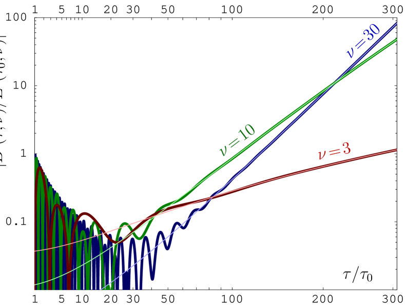
Figure 1: Numerical solution for individual magnetic modes $\widetilde{B}^{i}(\tau,\nu)$ normalized to $\widetilde{E}^{i}(\tau_{0},\nu)=\tau_{0}^{-1}\widetilde{\Pi}^{i}(\tau_{0},\nu)$ (thick dark lines) for $\tau_{0}/\tau_{\rm iso}=100$ and $c=0.5$ in a log-square root plot. Thin light lines give the analytical result of Eq.(21) with normalization to match the numerical result at late times. Note that $\tau_{0}^{-1}\simeq Q_{s}\simeq 1$ and 3 GeV for RHIC and LHC, resp. Iancu:2003xm .

In order to fix our dimensionful parameters in a way that makes contact with heavy-ion physics, we adopt the saturation scenario McLerran:1993ni ; Iancu:2003xm and assume that at $\tau_{0}\simeq Q_{s}^{-1}$ we have an initial hard-gluon density Baier:2002bt $n(\tau_{0})=2cQ_{s}^{3}/(3\pi^{2}\alpha_{s}Q_{s}\tau_{0})$, where $Q_{s}$ is the saturation scale. We consider two cases for the gluon liberation factor $c$: $c\simeq 0.5$ according to numerical simulations of Ref. Krasnitz:1998ns and $c=2\ln 2$ according to an approximate analytical calculation of Ref. Kovchegov:2000hz . Assuming further a deformed thermal distribution $f_{0}$ with $\tau_{\rm iso}\leq\tau_{0}$ and transverse temperature $T=Q_{s}/d$ with $d^{-1}=0.47$ taken from Ref. Iancu:2003xm , we obtain for a purely gluonic system $\mu/Q_{s}=cd\pi^{2}/[48\zeta(3)]\approx 0.182$ for $c=0.5$ and $\approx 0.505$ for $c=2\ln 2$. The amount of anisotropy at time $\tau_{0}$ is determined by the ratio $\tau_{0}/\tau_{\rm iso}$.

In Fig. 1 we display our numerical results for the magnetic field strength $\widetilde{B}^{i}(\tau,\nu)=\nu\tau^{-1}\,\widetilde{A}^{i}(\tau,\nu)$ with $c=0.5$ for $\nu=3,10,30$ and high initial anisotropy, $\tau_{0}/\tau_{\rm iso}=100$ (i.e., $\xi(\tau_{0})\sim 10^{4}$). For late times we observe a nearly perfect agreement with the analytical estimate of Eq.(21), which however does not contain information on the amplitudes of the unstable modes compared to their initial values. In the numerical evaluation we find that the modes with larger longitudinal momentum $\nu$, which have larger growth rates at late times, typically start to grow also only at larger proper times. This causes a certain delay for the onset of the instability which can be measured, e.g., by the time $\tau_{10}$ when the first of the modes $\widetilde{A}_{i}$ has grown in amplitude by a factor of 10 relative to its first maximum. For $\tau\geq\tau_{10}$ the dynamics of the collective modes is clearly dominated by the unstable modes. For times $\tau$ up to about half of $\tau_{10}$ we observe a decrease of the energy density carried by the unstable modes due to the expansion, but increase despite continued expansion thereafter. In Table 1 we list the values of $\tau_{10}$ that we found by scanning through $\nu$ with various initial anisotropies. Ideal-hydrodynamic fits to experimental data at RHIC indicate a life-time of a quark-gluon plasma of less than 5 fm/c $\simeq 30\,\tau_{0}$ Huovinen:2006jp . The values obtained in Table 1 turn out to be too large to suggest an important role of plasma instabilities in RHIC experiments if the gluon liberation factor $c\simeq 0.5$ as obtained in Ref. Krasnitz:1998ns ; Baier:2002bt . However, these unstable modes could contribute to fast isotropization of a quark-gluon plasma if the value of $c$ is much larger than those currently considered, or if the viscosity of the plasma is significant (in which case the life-time is increased Baier:2006um ). Finally, our results suggest that even for $c\simeq 0.5$, plasma instabilities will be an important phenomenon at the LHC, where plasma life-times might exceed 7 fm/c$\,\simeq 100\,\tau_{0}$ Eskola:2005ue .

Table 1: Approximate values of the proper time $\tau_{10}$ where the first of the modes $\widetilde{A}^{i}(\tau,\nu)$ has grown by a factor 10.

$\tau_{0}/\tau_{\rm iso}=\sqrt{\xi(\tau_{0})+1}$	1	10	100	1000
$\tau_{10}/\tau_{0}$ ($c=0.5$)	260	60	50	49
$\tau_{10}/\tau_{0}$ ($c=2\ln 2$)	95	25	21	20

To conclude, in this Letter we have laid the basis for numerical simulations of non-Abelian dynamics in heavy-ion collisions by generalizing the anisotropic but stationary hard-loop effective theory to the longitudinally expanding case. This opens the possibility of studying the fate of non-Abelian plasma instabilities in the highly nonlinear regime with expansion included. Moreover, we have determined the evolution of Weibel instabilities in a longitudinally expanding plasma in the regime where non-Abelian self-interactions of the unstable modes are negligible, finding that they start out oscillatory and later grow fast with an asymptotic behavior that we could determine analytically. Numerically, we have also been able to quantify the onset of this instability. Matching our dimensionful parameters to those of the saturation scenario we find that plasma instabilities overcome the effects of expansion at or after $\tau\sim 20Q_{s}^{-1}$ (which is roughly consistent with Ref.Romatschke:2005pm ). Unless initial parton densities are significantly higher than assumed here, only the prospected LHC experiments seem to offer large enough $Q_{s}$ and plasma life-times to generate strong quark-gluon-plasma instabilities from small rapidity fluctuations. The dynamics of strong initial fluctuations can only be determined by full nonlinear studies; this is work in progress.

References

(1)
J. Randrup and S. Mrówczyński, Phys. Rev. C 68, 034909 (2003);
S. Mrówczyński, hep-ph/0511052.
(2)
P. Romatschke and M. Strickland, Phys. Rev. D 68, 036004 (2003);
Phys. Rev. D 70, 116006 (2004).
(3)
P. Arnold, J. Lenaghan, and G. D. Moore, JHEP 08, 002 (2003);
P. Arnold, J. Lenaghan, G. D. Moore, and L. G. Yaffe, Phys. Rev. Lett. 94, 072302 (2005).
(4)
A. Rebhan, P. Romatschke, and M. Strickland, Phys. Rev. Lett. 94, 102303
(2005);
JHEP 09, 041 (2005).
(5)
A. Dumitru and Y. Nara, Phys. Lett. B621, 89 (2005);
A. Dumitru, Y. Nara and M. Strickland,
hep-ph/0604149.
(6)
P. Arnold, G. D. Moore, and L. G. Yaffe, Phys. Rev. D 72, 054003 (2005).
(7)
L. D. McLerran and R. Venugopalan, Phys. Rev. D 49, 2233, 3352 (1994); 50, 2225 (1994).
(8)
E. Iancu and R. Venugopalan, hep-ph/0303204.
(9)
E. S. Weibel, Phys. Rev. Lett. 2, 83 (1959).
(10)
S. Mrówczyński, A. Rebhan, and M. Strickland, Phys. Rev. D 70,
025004 (2004).
(11)
P. Arnold and G. D. Moore, Phys. Rev. D 73, 025006 (2006);
Phys. Rev. D 73, 025013 (2006).
(12)
M. Asakawa, S. A. Bass, and B. Müller,
Phys. Rev. Lett. 96, 252301 (2006).
(13)
A. H. Mueller, Phys. Lett. B475, 220 (2000).
(14)
R. Baier, A. H. Mueller, D. Schiff, and D. T. Son, Phys. Lett. B539, 46
(2002).
(15)
P. Romatschke and R. Venugopalan, Phys. Rev. Lett. 96, 062302
(2006);
Eur. Phys. J. A 29, 71 (2006);
Phys. Rev. D 74, 045011 (2006).
(16)
J.-P. Blaizot and E. Iancu, Phys. Rept. 359, 355 (2002).
(17)
A. Krasnitz and R. Venugopalan, Nucl. Phys. B557, 237 (1999);
Nucl. Phys. A698, 209 (2002);
T. Lappi, Phys. Rev. C 67, 054903 (2003).
(18)
Y. V. Kovchegov, Nucl. Phys. A692, 557 (2001).
(19)
P. Huovinen and P. V. Ruuskanen, nucl-th/0605008.
(20)
R. Baier, P. Romatschke, and U. A. Wiedemann, Phys. Rev. C 73 064903 (2006).
(21)
K. J. Eskola et al., Phys. Rev. C 72 (2005) 044904.