Baryon Stopping in Proton-Nucleus Collisions

Abstract

We calculate the inclusive small-$x$ valence quark production cross section in proton-nucleus collisions at high energies. The calculation is performed in the framework of the Color Glass Condensate formalism. We consider both the case when the valence quark originates inside the nucleus and the case when it originates inside the proton. We first calculate the cross section in the quasi-classical approximation resumming the multiple rescatterings with the nucleus. Then we include the the effects of double logarithmic reggeon evolution and leading logarithmic gluon evolution in the obtained cross section. The calculated nuclear modification factor for the stopped baryons exhibits Cronin enhancement in the quasi-classical approximation and suppression at high energies/rapidities when quantum evolution corrections are included, providing a new observable which can be used to test Color Glass physics.

1 Introduction

One of the most striking features of experimental data in nuclear collisions at high energies is the large stopping suffered by the nucleons entering the collision [1, 2, 3]. This stopping translates into a net baryon number transfer from the forward to the central rapidity region, and has already been observed in proton-nucleus and nucleus-nucleus collisions at CERN [1, 2] and in $Au+Au$ collisions at RHIC [3]. The description of this phenomenon has been previously approached in the framework of non-perturbative models for hadron collisions [4, 5, 6, 7, 8]. In [4, 5, 6, 7, 8] the baryon number transfer along a large rapidity gap is attributed to topological excitations of the gluon field.

In this work, following [9], we consider the problem of baryon stopping from a purely perturbative perspective in which the carriers of baryon number are the energetic valence quarks entering the collision, that loose much of their longitudinal momenta in the collision and are driven towards the central rapidity region via hard gluon emissions. Valence quark production in the scattering of a proton on a nucleus is calculated in the framework of the Color Glass Condensate (CGC) formalism [10, 11, 12, 13, 14, 15, 16, 17, 18]. The effects of strong gluonic fields in the small-$x$ hadronic or nuclear wave functions on baryon number transfer were first considered by one of the authors with collaborators in [9]. The valence quark distribution at small Bjorken $x$ was first studied in [9] in the quasi-classical approximation of McLerran-Venugopalan model [11]. Quantum evolution corrections come into the obtained valence quark distribution through a non-linear evolution equation which was derived in [9]. The linear part of the evolution equation from [9] corresponds to the well-known double logarithmic reggeon evolution equation from [19, 20, 21, 22]. It is an interesting property of quark evolution that at the leading order each power of the coupling constant $\alpha_{s}$ is accompanied by two powers of the logarithm of center-of-mass energy $\ln s$, or, equivalently, of the logarithm $\ln 1/x$ of inverse Bjorken $x$ [19, 20, 21, 22]. The resummation parameter is thus $\alpha_{s}\,\ln^{2}1/x$, unlike, say, the BFKL equation [23], which resums powers of $\alpha_{s}\,\ln 1/x$. Due to that property one may expect the small-$x$ evolution corrections to manifest themselves earlier (i.e., at larger values of $x$ and smaller rapidities) in observables related to valence quarks. The non-linear part of the evolution equation derived in [9] is due to gluon evolution effects, similar to those resummed in [15, 16, 17, 18]. While the linear reggeon evolution [19, 20, 21, 22] tends to increase the small-$x$ valence quark distribution, the effect of nonlinear evolution equation [9] is to reduce the valence quark distribution at very small-$x$ as compared to the linear evolution predictions.

Here we continue the work done in [9] by calculating the inclusive production cross section for small-$x$ valence quarks in $pA$ collisions. We perform the calculations both in the quasi-classical approximation [11, 12] and including quantum evolution from [9]. We use the techniques for calculation of inclusive cross sections developed in [24, 25] (for a review see [26]). The calculation of inclusive gluon production in pA collisions was performed in [24, 27] in the quasi-classical approximation and in [25] the effects of quantum evolution were included in the cross section. Our calculations will proceed along similar lines. In Section 2 we derive the expression for valence quark production in the quasi-classical approximation resumming multiple rescatterings of the incoming proton and produced valence quark on the nucleons in the target nucleus. Here one has to separately consider two cases: the valence quark may originate either in the proton or in the nucleus. The stopping of valence quarks in these two cases is clearly distinguishable experimentally: the rapidity distribution of stopped valence quarks from the proton scales as $\sim e^{y-Y}$ while the valence quarks from the nucleus are distributed as $\sim e^{-y}$. (Here the nucleus has rapidity $0$, the proton has rapidity $Y$ and the quark is produced at rapidity $y$.) We calculate both contributions in Sect 2.1 and study their properties in Sect 2.2. Our results here are complimentary to the valence quark production calculated in [28]: the authors of [28] considered production of a hard valence quark which experiences no recoil and is produced in the fragmentation region, while here we are interested in production of a soft valence quark far away (in rapidity) from the fragmentation region.

As was shown in [29, 30, 31, 32, 33, 34, 35, 36, 37] for gluons, multiple rescatterings in the nucleus lead to enhancement of high-$p_{T}$ particle production which is similar to the Cronin effect observed in [38]. Analyzing the nuclear modification factor resulting from the derived quasi-classical cross section for valence quark production, we observe that valence quarks also exhibit Cronin enhancement, as demonstrated in Fig. 5.

We continue in Section 3 by including the effects of non-linear reggeon evolution from [9] into the valence quark production cross section. The cases of valence quark originating in the proton and in the nucleus are considered separately in Sections 3.1 and 3.3. Similar to the case of gluon production [25], the evolution between the produced quark and the projectile turns out to be linear and is given by the reggeon evolution equation [19] if the quark comes from the proton and by the BFKL equation [23] if the quark comes from the nucleus. The evolution between the produced valence quark and the target nucleus is always non-linear.

As was originally observed in [39, 29, 30] for gluon production, small-$x$ evolution introduces suppression in the nuclear modification factor at high energies/rapidities, turning Cronin enhancement into suppression. These predictions were confirmed by the forward rapidity particle production data produced by RHIC $d+Au$ experiments [40, 41, 42, 43, 44]. In Section 3.2 we study the effects of non-linear reggeon evolution on valence quark nuclear modification factor for the case when the valence quarks are produced from the proton. We observe suppression of nuclear modification factor which increases with rapidity/energy similar to the case of the gluons, as shown in Fig. 7. Therefore, if baryon stopping is dominated by perturbative mechanisms, we expect the nuclear modification factor for net baryons to be suppressed at forward rapidities in $d+Au$ collisions at RHIC. Thus the nuclear modification factor for stopped baryons may serve as a new test of Color Glass Condensate (CGC) dynamics in nuclear collisions, or, at least it may help determine the relative contributions of perturbative and non-perturbative baryon stopping.

We conclude in Section 4 by discussing the applicability of obtained results and the prospects for experimental testing of the derived formulas. In order to compare our results to the actual experimental data produced at RHIC and to make predictions for the LHC, as was done in [45, 46, 47, 48], one should implement the fragmentation mechanism which converts valence quarks into hadrons. This goes beyond the scope of this paper and is left for future work.

2 Valence Quark Production in the Quasi-Classical Approximation

2.1 Derivation of the Expression for the Production Cross Section

We are interested in calculating the soft valence quark spectrum in proton-nucleus collisions at high energies. In what follows we will assume that the proton is moving ultrarelativistically in the light-cone ’plus’ direction and, consequently, has a large $p_{1}^{+}$ momentum component, whereas a nucleon in the nucleus is moving in the light-cone ’minus’ direction with a large $p_{2}^{-}$ momentum component. We employ Sudakov parameterization for the light-cone components of the momentum of the the produced valence quark: $k=(\alpha\,p_{1}^{+},\beta\,p_{2}^{-},\underline{k})$. In the center of mass frame of the collision, the relation of the dimensionless Sudakov parameters $\alpha$ and $\beta$ to the rapidity of the produced quark $y$ and the total rapidity of the collision $Y$ is

$$\alpha\,=\,\frac{|\underline{k}|}{\sqrt{s}}e^{y-Y/2},\qquad\beta\,=\,\frac{|\underline{k}|}{\sqrt{s}}e^{-y+Y/2}\,,$$ (1)

where $s=2p_{1}^{+}\,p_{2}^{-}$ is the square of the center-of-mass energy of the collision and the proton has rapidity $y=Y$ while the target nucleus has $y=0$. The calculation below will be performed in the light-cone gauge of the proton, $A^{+}=0$, which for the nucleus moving in the ’minus’ direction is equivalent to the covariant gauge, $\partial\cdot A=0$. This choice completely determines the set of diagrams that are relevant for our calculation as well as their physical interpretation: As it was discussed in detail in [24, 51], in this gauge the classical current associated with the nucleus, $J^{-}$, remains unchanged throughout the collision and the nuclear effects become manifest in the form of multiple scatterings between the nucleons in the nucleus and the rest of the system.

As usual at high energies, the resummation of the multiple rescatterings is performed in the eikonal approximation, in which the energetic projectiles (quark or gluon) remain at fixed transverse coordinate as they propagate through nuclear matter. Hence the calculation is done in coordinate space. Besides, we restrict the interactions with the nucleons in the nucleus to two-gluon exchanges, in the spirit of the quasi-classical approximation. More technically this implies that the resummation parameter is $\alpha_{s}^{2}A^{1/3}$, with $A$ the atomic number of the nucleus. We are assuming that the energy of the collision is large enough for an eikonal description of the multiple rescatterings to be appropriate, but not large enough for quantum corrections to become important. Under these two approximations (eikonal limit and quasi-classical description) the effects of multiple rescatterings, and therefore all the nuclear effects, can be recast in the form of Glauber-Mueller propagators [24, 55].

We divide the cross section for soft quark production into two terms: the first contribution, labeled (a), corresponds to produced valence quark coming from the proton, while the second one, labeled (b), corresponds to valence quark coming from one of the nucleons in the nucleus via interaction with a soft gluon in the proton wavefunction (see below):

$$\frac{d\sigma}{d^{2}k\,dy}=\frac{d\sigma^{a}}{d^{2}k\,dy}+\frac{d\sigma^{b}}{d^{2}k\,dy}.$$ (2)

Importantly, the formation time associated with the soft valence quark production mechanism is, in both cases, much longer than the typical time scale for the nucleus-proton interactions, which can be considered instantaneous. Moreover, the diagrams in which the soft valence quark emission happens during the interaction with the nucleus are suppressed by powers of the total energy of the collision and, therefore, can be neglected in the high energy limit. This allows us to deal with time-ordered diagrams or, more precisely, the calculation is more convenient (and will be done) in the framework of time-ordered light-cone perturbation theory [53].

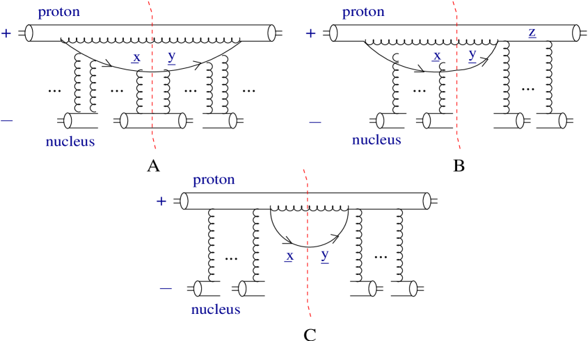
Figure 1: Diagrams corresponding to the first contribution to the cross section as considered in the text, where the produced valence quark originates in the proton.

First we are going to find the contribution to the cross section in which the produced soft valence quark originates in the proton wavefunction. The contributing diagrams are shown in Fig. 1. The discussion here will proceed along the lines of the calculation done in [24] of the gluon production in pA collisions. The physical picture is the following: one of the fast valence quarks in the proton has to emit a hard gluon in order to loose most of its large longitudinal momentum and, therefore, become soft. This splitting is given by the soft-quark wavefunction of the proton at the lowest order in perturbation theory (see appendix A):

$$\psi^{a}_{\sigma,\lambda}(\underline{x},\underline{z},\alpha)=gt^{a}[1-\sigma\lambda]\,\frac{i}{2\pi}\,\frac{(\underline{x}-\underline{z})\cdot\underline{\epsilon}^{\lambda}}{(\underline{x}-\underline{z})^{2}}\,,$$ (3)

where $\underline{z}$ is the transverse coordinate of the hard gluon (which is equal to the transverse coordinate of the fast quark), $\underline{x}$ is the transverse coordinate of the soft quark, $\sigma$ is the helicity of the fast quark, $a$ and $\lambda$ are the color and polarization of the hard gluon. The helicity of the soft quark is equal to the one of the fast one due to helicity conservation for massless quarks.

Analogously to what was done in [9], it is convenient to introduce the soft quark distribution of a proton. In order to do so we multiply the above wavefunction in Eq. (3) by its complex conjugate evaluated at transverse position $\underline{y}$, average over the helicity of the initial quark and sum over the polarization and color of the hard gluon, getting

$$\frac{dn^{q}}{d^{2}z\,dy}\,=\,\frac{1}{4\pi}\,\frac{\alpha}{2}\,\sum_{\sigma,\lambda,a}\langle\psi^{a}_{\sigma,\lambda}(\underline{x},\underline{z},\alpha)\psi^{*a}_{\sigma,\lambda}(\underline{y},\underline{z},\alpha)\rangle=\frac{\bar{\alpha}_{s}\,\alpha\,N_{c}}{2\pi}\,\frac{(\underline{x}-\underline{z})\cdot(\underline{y}-\underline{z})}{(\underline{x}-\underline{z})^{2}(\underline{y}-\underline{z})^{2}}\,,$$ (4)

where $\bar{\alpha}_{s}=\alpha_{s}C_{F}/\pi$. The factor of $N_{c}$ on the right hand side of Eq. (4) accounts for the three valence quarks in a proton. All the dynamics corresponding to the soft-quark emission in the diagrams we are going to calculate is included in the distribution in Eq. (4).

Our next step is to resum the multiple rescatterings of the quark-gluon system in the nucleus. The diagram shown in Fig. 1A corresponds to the case in which the incoming proton has already developed a soft valence quark component in its wavefunction before interacting with the nucleus both in the amplitude and in its complex conjugate. As is explicitly shown in Fig. 1A, in this case only the interactions between the nucleons and the soft-quark line survive. The interactions between the nucleons and the hard gluon vanish due to real-virtual cancellation [24]. This can be understood in the following terms: since we want to keep the momentum of the produced soft valence quark fixed, in the transverse coordinate space that we are going to perform our calculation in, its transverse coordinate in the amplitude $\underline{x}$ has to be different from the one in the complex conjugate amplitude $\underline{y}$ [24, 26]. The transverse momenta of all other particles in the final state are integrated over (inclusive production) making their coordinates in the amplitude and in the complex conjugate amplitude equal to each other. Therefore, one can freely move the $t$-channel gluon lines connecting the nucleons with the hard gluon across the cut without changing either the color factor or the momentum of the produced quark, but picking up a relative minus sign in the way, which provides the cancellation.

To calculate the surviving contribution one can proceed either by direct evaluation of the diagrams or, alternatively, by making use of the crossing symmetry property [54, 26] in the following way: mirror-reflecting the soft quark line in the complex conjugate amplitude of Fig. 1A with respect to the final state cut one is left with the diagram corresponding to the amplitude of a quark-antiquark dipole of transverse size $|\underline{x}-\underline{y}|$ multiply scattering off a nucleus. The amplitude for this process is [55]

$$N(\underline{x},\underline{y})\,=\,1-e^{-|\underline{x}-\underline{y}|^{2}Q_{sq}^{2}\ln(1/|\underline{x}-\underline{y}|\Lambda)/4},$$ (5)

where

$$Q_{sq}^{2}=4\pi\,{\alpha}_{s}^{2}\,\frac{C_{F}}{N_{c}}\,\rho\,T_{A}(\underline{b})$$ (6)

is the saturation scale of a quark dipole, $\rho$ is the nuclear density (normalized to $A$) and $T_{A}(\underline{b})$ is the nuclear thickness at impact parameter $\underline{b}$ in its own rest frame, which for a spherical nucleus of radius $R$ is equal to $T_{A}(\underline{b})=2\sqrt{R^{2}-\underline{b}^{2}}$.

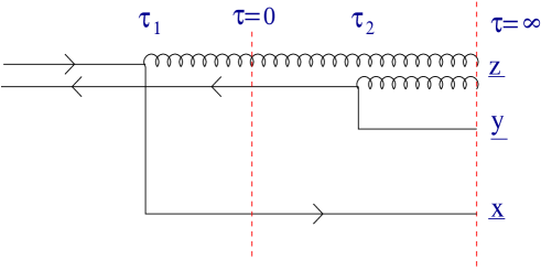
Figure 2: Mirror reflection of the diagram in Fig. 1B. $\tau_{1(2)}$ is the emission time in the amplitude (complex conjugate amplitude). The interaction time is $\tau=0$, represented in the figure by a vertical line and the final state cut is denoted by $\tau=+\infty$.

The diagram in which the soft quark is emitted before the interaction with the nucleus in the amplitude, but after the interaction in the complex conjugate one is shown in Fig. 1B. The interactions between the nucleus and the hard gluon line in the amplitude do not cancel in this case since, to move the gluon line attached to the fast quark in the complex conjugate amplitude across the cut, one is forced to ’jump’ over the emission vertex, which would modify the momentum of the produced quark, ruining the cancellation. To explicitly include both the interactions with the $s$-channel quark and gluon lines, we do not connect the $t$-channel gluon lines to any particular line in Fig. 1B. Again, mirror-reflecting the complex conjugate amplitude with respect to the cut generates the configuration represented in Fig. 2. There, the fast valence quark line in the complex conjugate amplitude turns into an antiquark line overlapping the hard gluon line in the amplitude at transverse coordinate $\underline{0}$. Since the whole system is color neutral, the zero-size antiquark-gluon system has to be in the $\bar{3}$ representation of $SU(3)$, which together with the quark line located at the $\underline{x}$ coordinate is equivalent to a quark dipole multiply rescattering off a nucleus. Therefore, the factor entering the production cross-section due to interactions in Fig. 1B is

$$N(\underline{x},\underline{z})=1-e^{-|\underline{x}-\underline{z}|^{2}Q_{sq}^{2}\ln(1/|\underline{x}-\underline{z}|\Lambda)/4}.$$ (7)

The contribution of the diagram complex conjugate to Fig. 1B (not shown) is calculated in an analogous way yielding

$$N(\underline{y},\underline{z})=1-e^{-|\underline{y}-\underline{z}|^{2}Q_{sq}^{2}\ln(1/|\underline{y}-\underline{z}|\Lambda)/4}.$$ (8)

The diagram in Fig. 1C gives a zero contribution to the production cross-section, since, due to real-virtual cancellations, all the interactions with the target cancel, leading to $N=0$.

Finally, adding up the contributions to the production cross sections of the diagrams in Fig. 1 gives

$$\frac{d\sigma^{a}}{d^{2}k\,dy}=\frac{1}{(2\pi)^{2}}\,\int\!d^{2}x\,d^{2}y\,d^{2}z\,e^{i\underline{k}(\underline{x}-\underline{y})}\,\frac{dn^{q}}{d^{2}z\,dy}$$

$$\times\,\left[e^{-(\underline{x}-\underline{y})^{2}Q_{sq}^{2}\ln(1/|\underline{x}-\underline{y}|\Lambda)/4}-e^{-(\underline{x}-\underline{z})^{2}Q_{sq}^{2}\ln(1/|\underline{x}-\underline{z}|\Lambda)/4}-e^{-(\underline{y}-\underline{z})^{2}Q_{sq}^{2}\ln(1/|\underline{y}-\underline{z}|\Lambda)/4}+1\right].$$ (9)

Our next step is to calculate the diagram in which the produced valence quark originates in the nucleus wavefunction, an example of which is shown in Fig. 3. Before starting this calculation, let us discuss the diagrams that do not contribute to the cross-section in this case. First, the emission of the hard gluon cannot happen via interaction with any other nucleon in the nucleus. In its rest frame the nucleus is a dilute system, i.e, its constituents nucleons are spatially separated from each other. In a frame in which the nucleus is fast moving in the light-cone ’minus’ direction, diluteness of the nucleus translates into the fact that the nucleons are strongly localized around fixed well differentiated $x^{+}$ coordinates: $x_{1}^{+}<x_{2}^{+}\dots<x_{A}^{+}$. Moreover, the gluon field of the nucleus as given by the classical equations of motion in the $A^{+}=0$ gauge is equivalent to the gluon field in covariant gauge and is strongly localized around the $x^{+}$ coordinates of the nucleons [55, 12]: $\underline{A}\sim\Sigma_{i}\delta(x^{+}-x^{+}_{i})$. Therefore, the interactions between the nucleons are suppressed by powers of $A$. In the leading order in $\alpha_{s}^{2}A^{1/3}$ calculation, corresponding to the quasi-classical limit used here, the nucleons can be assumed as not interacting with each other. On the other hand, those diagrams in which a nucleon exchanges one gluon with one of the quarks in the proton and subsequently emits a hard gluon are suppressed by a power of center-of-mass energy at high energies in $A^{+}=0$ light-cone gauge and are also subleading. This leaves us with a single possibility for the nucleon’s valence quark to be produced at central rapidity: it may only happen via interaction with a soft gluon in the proton’s wavefunction, as shown in Fig. 3.

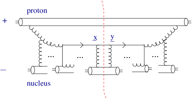
Figure 3: Valence quark production diagram corresponding to the second case considered in the text, where the produced soft valence quark originates from the nuclear wave function.

The physics is clear: the proton has to emit a soft gluon before its interaction with the nucleus. This emission is given by the soft-gluon wavefunction of a valence quark

$$\psi^{a}_{\sigma,\lambda}(\underline{x},\underline{z})\,=\,2\,g\,t^{a}\,\frac{i}{2\pi}\frac{(\underline{x}-\underline{z})\cdot\underline{\epsilon}^{\lambda}}{(\underline{x}-\underline{z})^{2}}\,.$$ (10)

The emitted soft gluon undergoes multiple rescatterings until being absorbed by one of the valence quarks of the ith nucleon at the longitudinal coordinate $u$. This way, the valence quark is kicked out from its original light-cone trajectory towards the central rapidity region and is likely to rescatter on the remaining nucleons in the nucleus. A space-time picture of the collision is depicted in Fig. 4A. Integrating over the longitudinal coordinate $u$ and summing over all nucleons in the nucleus one gets the following factor:

$$\rho\int_{0}^{L}\!\!du\,e^{-(\underline{x}-\underline{y})^{2}Q_{sg}^{2}\ln(1/|\underline{x}-\underline{y}|\Lambda)u/4L}\,\hat{V}(\underline{x},\underline{y})\,e^{-(\underline{x}-\underline{y})^{2}Q_{sq}^{2}\ln(1/|\underline{x}-\underline{y}|\Lambda)(L-u)/4L}.$$ (11)

The first exponential term in Eq. (11) accounts for the propagation of a gluon dipole until the longitudinal coordinate $u$ (see Fig. 4B) with

$$Q_{sg}^{2}=4\pi\alpha_{s}^{2}\rho T_{A}(\underline{b})$$ (12)

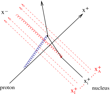
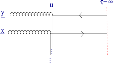
Figure 4: Space-time picture of the diagram in Fig. 3 (left), and its mirror reflection (right):

the gluon dipole saturation scale. The factor $\hat{V}(\underline{x},\underline{y})$ is the Fourier transform of the ${Gq\rightarrow qG}$ cross-section in the high energy limit (see Appendix B for a detailed derivation):

$$\hat{V}(\underline{x},\underline{y})=N_{c}\,\int\!d^{2}{l}\,e^{i\underline{l}\cdot(\underline{x}-\underline{y})}\frac{d\sigma^{Gq\rightarrow qG}}{d^{2}{l}}=\pi\alpha_{s}^{2}C_{F}\frac{1}{\hat{s}}\ln\frac{1}{(\underline{x}-\underline{y})^{2}\Lambda^{2}},$$ (13)

where $\hat{s}=2k^{+}p_{2}^{-}=|{\underline{k}}|\sqrt{s}\,e^{y-\frac{Y}{2}}$. The factor of $N_{c}$ entering the definition of $\hat{V}$ accounts for the three valence quarks in a nucleon. Finally, the second exponential term in Eq. (11) corresponds to the propagation of a quark dipole from $u$ till the edge of the nucleus $L$, which is equal to $T_{A}(b)$ evaluated at a fixed value of the impact parameter. Thus, the contribution to the cross section of the diagram in Fig. 3 is:

$$\frac{d\sigma^{b}}{d^{2}k\,dy}\,=\,\frac{1}{(2\pi)^{2}}\,\int\!d^{2}x\,d^{2}y\,d^{2}z\,e^{i\underline{k}(\underline{x}-\underline{y})}\,\frac{dn^{g}}{d^{2}z\,dy}$$

$$\times\,\left[\rho\int_{0}^{L}\!\!du\,e^{-(\underline{x}-\underline{y})^{2}Q_{sg}^{2}\ln(1/|\underline{x}-\underline{y}|\Lambda)u/4L}\,\hat{V}(\underline{x},\underline{y})\,e^{-(\underline{x}-\underline{y})^{2}Q_{sq}^{2}\ln(1/|\underline{x}-\underline{y}|\Lambda)(L-u)/4L}\right]\,,$$ (14)

where

$$\frac{dn^{g}}{d^{2}z\,dy}=\frac{\bar{\alpha}_{s}}{\pi}\,\frac{(\underline{x}-\underline{z})\cdot(\underline{y}-\underline{z})}{(\underline{x}-\underline{z})^{2}(\underline{y}-\underline{z})^{2}},$$ (15)

is the soft gluon distribution of the valence quark.

Rewriting $\alpha$ in Eq. (9) and $\beta$ in Eq. (14) using Eqs. (1), performing the integral over the longitudinal coordinate $u$ in Eq. (14) and shifting the integration variables in the following way

$$\underline{x}-\underline{z}\equiv\underline{x},$$ (16)

$$\underline{y}-\underline{z}\equiv\underline{y},$$ (17)

$$\underline{z}\equiv\underline{b},$$ (18)

the final result for the soft valence quark production cross section in the quasi-classical approximation can be rewritten as:

$$\frac{d\sigma}{d^{2}k\,dy}\,=\,\frac{d\sigma^{a}}{d^{2}k\,dy}+\frac{d\sigma^{b}}{d^{2}k\,dy},$$ (19)

with

$$\frac{d\sigma^{a}}{d^{2}k\,dy}=\frac{1}{(2\pi)^{2}}\frac{\bar{\alpha}_{s}\,N_{c}}{2\pi}e^{y-Y/2}\,\frac{|\underline{k}|}{\sqrt{s}}\int\!d^{2}x\,d^{2}y\,d^{2}b\,e^{i\underline{k}(\underline{x}-\underline{y})}\,\frac{\underline{x}\cdot\underline{y}}{\underline{x}^{2}\underline{y}^{2}}$$

$$\times\,\left[e^{-(\underline{x}-\underline{y})^{2}Q_{sq}^{2}\ln(1/|\underline{x}-\underline{y}|\Lambda)/4}-e^{-\underline{x}^{2}Q_{sq}^{2}\ln(1/|\underline{x}|\Lambda)/4}-e^{-\underline{y}^{2}Q_{sq}^{2}\ln(1/|\underline{y}|\Lambda)/4}+1\right],$$ (20)

and

$$\frac{d\sigma^{b}}{d^{2}k\,dy}=\frac{1}{(2\pi)^{2}}\frac{2\bar{\alpha}_{s}}{\pi}\frac{C_{F}}{1-\frac{C_{F}}{N_{c}}}\frac{e^{-y+Y/2}}{\sqrt{s}|\underline{k}|}\,\int\!d^{2}x\,d^{2}y\,d^{2}b\,e^{i\underline{k}(\underline{x}-\underline{y})}\,\frac{\underline{x}\cdot\underline{y}}{\underline{x}^{2}\underline{y}^{2}}\,\frac{1}{(\underline{x}-\underline{y})^{2}}$$

$$\times\,\left[e^{-(\underline{x}-\underline{y})^{2}Q_{sq}^{2}\ln(1/|\underline{x}-\underline{y}|\Lambda)/4}-e^{-(\underline{x}-\underline{y})^{2}Q_{sg}^{2}\ln(1/|\underline{x}-\underline{y}|\Lambda)/4}\right].$$ (21)

In arriving at Eq. (21) we have used the definition of the saturation scale from Eqs. (6) and (12) with $T_{A}(b)$ replaced by $L$.

Equations (19), (20) and (21) provide the result for the small-x valence quark production in pA collisions at high energies in the quasi-classical approximation.

2.2 Properties of the Quasi-Classical Cross Section

In this Section we explore some of the properties of the valence quark production cross section derived in the previous Section.

First let us consider the case of $k_{T}\ll Q_{s}$, where $k_{T}=|\underline{k}|$. For momenta of the produced quark much smaller than the saturation scale, $k_{T}\ll Q_{s}$, the dynamics is governed by the strong nuclear effects. In this region the integrals in Eqs. (20) and (21) are dominated by large distances and setting the logarithms in the exponentials to a constant value (more precisely to $1$) is a good approximation. This way the integrals are analytically doable, yielding

$$\frac{d\sigma^{a}}{d^{2}k\,dy}=\frac{\bar{\alpha_{s}}N_{c}}{2\pi}\frac{e^{y-Y/2}}{\sqrt{s}}\int\!d^{2}{b}\,\left\{-\frac{1}{|\underline{k}|}+\frac{2}{|\underline{k}|}e^{-\underline{k}^{2}/Q_{sq}^{2}}+|\underline{k}|\frac{e^{-\underline{k}^{2}/Q_{sq}^{2}}}{Q_{sq}^{2}}\left[\mbox{Ei}\left(\frac{\underline{k}^{2}}{Q_{sq}^{2}}\right)+\ln\frac{Q_{sq}^{4}}{4\underline{k}^{2}\Lambda^{2}}\right]\right\},$$ (22)

and

$$\frac{d\sigma^{b}}{d^{2}k\,dy}=\frac{\bar{\alpha_{s}}}{2\pi}\frac{C_{F}}{1-\frac{C_{F}}{N_{c}}}\,\frac{e^{-y+Y/2}}{\sqrt{s}}\frac{1}{|\underline{k}|}\int\!d^{2}\underline{b}\left\{\left(\ln\frac{Q_{sg}^{2}}{4\Lambda^{2}}+\gamma_{E}\right)\left[\Gamma\left(0,\frac{\underline{k}^{2}}{Q_{sg}^{2}}\right)+\ln\frac{\underline{k}^{2}}{Q_{sg}^{2}}\right]\right.$$

$$-\left.\left(\ln\frac{Q_{sq}^{2}}{4\Lambda^{2}}+\gamma_{E}\right)\left[\Gamma\left(0,\frac{\underline{k}^{2}}{Q_{sq}^{2}}\right)+\ln\frac{\underline{k}^{2}}{Q_{sq}^{2}}\right]\right\},$$ (23)

where Ei is the exponential integral function and $\Gamma$ is the incomplete gamma function.

On the other hand, for very large transverse momenta, $k_{T}\gg Q_{s}$, the nuclear effects are absent (tend to disappear) and the perturbative result should be recovered. Expanding the exponentials in Eq. (9) and Eq. (14) one gets the following expansion in powers of $Q_{sq}/k_{T}$ (“twists”):

$$\frac{d\sigma^{a}}{d^{2}k\,dy}=\frac{\bar{\alpha_{s}}N_{c}}{2\pi}\frac{e^{y-Y/2}}{\sqrt{s}}\int\!d^{2}{b}\frac{Q_{sq}^{2}}{k_{T}^{3}}\left\{\left[\ln\frac{\underline{k}^{2}}{4\Lambda^{2}}+2\gamma_{E}-1\right]+\frac{Q_{sq}^{2}}{k_{T}^{2}}\left[\frac{3}{2}\ln^{2}\frac{\underline{k}^{2}}{4\Lambda^{2}}\right.\right.$$

$$\left.\left.+2\ln\frac{\underline{k}^{2}}{4\Lambda^{2}}(3\gamma_{E}-4)+6\gamma_{E}^{2}-16\gamma_{E}+\frac{29}{4}\right]+\dots\right\},$$ (24)

and

$$\frac{d\sigma^{b}}{d^{2}k\,dy}=\frac{\bar{\alpha_{s}}N_{c}}{2\pi}\,\frac{e^{-y+Y/2}}{\sqrt{s}}\int d^{2}{b}\,\frac{Q_{sq}^{2}}{k_{T}^{3}}\left\{\left[\ln\frac{\underline{k}^{2}}{4\Lambda^{2}}+2\gamma_{E}\right]+\frac{Q_{sq}^{2}}{k_{T}^{2}}\left(\frac{N_{c}}{C_{F}}+1\right)\left[\frac{3}{8}\ln^{2}\frac{\underline{k}^{2}}{4\Lambda^{2}}\right.\right.$$

$$\left.\left.+\frac{3}{2}\ln\frac{\underline{k}^{2}}{4\Lambda^{2}}(\gamma_{E}-1)+\frac{2}{3}(2\gamma_{E}^{2}-4\gamma_{E}+1)\right]+\dots\right\}.$$ (25)

Remarkably, at large transverse momentum and fixed rapidity the valence quark production cross section scales like $\sim 1/k_{T}^{3}$, which is to be compared with the $\sim 1/k_{T}^{4}$ scaling of the inclusive gluon production cross section. As is well-known, the quark production cross section turns out to be more sensitive to the ultraviolet.

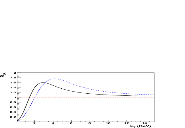
Figure 5: Nuclear modification factor at central rapidity for $Q_{sq}^{2}=1$ GeV² (solid) and $Q_{sq}^{2}=2$ GeV² (dashed). The cutoff is $\Lambda=0.1\,Q_{sq}$.

To study the transition between the small and large transverse momentum regions and to have a quantitative measure of the nuclear effects we introduce the nuclear modification factor, equal to the ratio of the valence quark production cross section in $pA$ collisions over the one in $pp$ collisions scaled by the number of binary collisions

$$R_{pA}(y,k_{T})=\frac{\frac{d\sigma^{pA}}{d^{2}k\,dy}}{A\,\frac{d\sigma^{pp}}{d^{2}k\,dy}}\,.$$ (26)

The cross section for proton-proton collisions can be obtained as a particular case of our calculation, just keeping the first terms in the twist expansions of Eqs. (24) and (25) and setting $A=1$. We get

$$A\,\frac{d\sigma^{pp}}{d^{2}k\,dy}\,\approx\,\frac{\bar{\alpha_{s}}N_{c}}{\pi}\,\frac{\cosh(y-Y/2)}{\sqrt{s}}\int\!d^{2}{b}\,\frac{Q_{sq}^{2}}{k_{T}^{3}}\,\ln\frac{\underline{k}^{2}}{4\Lambda^{2}}\,,$$ (27)

where we have used $Q_{sq}^{2}\sim A^{1/3}$ and the fact that, for a cylindrical nucleus, the integral over impact parameter gives just a factor of the transverse area of the nucleus, $S_{A}\sim A^{2/3}$. In what follows we will restrict our discussion about $R_{pA}$ to the central rapidity region, $y=Y/2$. The limiting behavior of $R_{pA}$ at momenta $k_{T}\ll Q_{sq}$ can be obtained by expanding Eq. (22) and Eq. (23) in powers of $k_{T}/Q_{sq}$, yielding

$$R_{pA}(y=Y/2,k_{T}\ll Q_{sq})\approx\frac{\underline{k}^{2}}{Q_{sq}^{2}}+\frac{\underline{k}^{4}}{Q_{sq}^{4}}\bigg{(}\gamma_{E}+\ln\frac{Q_{sq}^{2}}{4\,\Lambda^{2}}+\frac{N_{c}}{1-\frac{C_{F}}{N_{c}}}\,\ln\frac{N_{c}}{C_{F}}-2\bigg{)}+\dots<1,$$ (28)

indicating that deep in the saturation region the valence quark production is suppressed due to nuclear effects and that $R_{pA}$ increases with increasing momentum. On the other hand, from Eq. (24), Eq. (25) and Eq. (27) we derive the limiting behavior at large momentum, $k_{T}\gg Q_{sq}$,

$$R_{pA}(y=Y/2,k_{T}\gg Q_{sq})\approx 1+\frac{15}{8}\frac{Q_{sq}^{2}}{\underline{k}^{2}}\ln^{2}\frac{\underline{k}^{2}}{4\Lambda^{2}}+\dots>1,$$ (29)

which shows that $R_{pA}$ approaches unity from above at asymptotically large transverse momentum. Therefore $R_{pA}$ must reach a maximum value at intermediate momentum $k_{T}\sim Q_{sq}$, as it is shown in Fig. 5, where we plot the nuclear modification factor $R_{pA}$ at mid-rapidity ($y=Y/2$) built up by evaluating the integrals in Eq. (20) and Eq. (21) numerically for two different values of the quark saturation scale.

We therefore conclude that, in the framework of the quasi-classical approximation, the nuclear modification factor for small-$x$ valence quark production in the central rapidity region is less than 1 at $k_{T}<Q_{sq}$ and has a Cronin enhancement at high $k_{T}\sim Q_{sq}$. An equivalent (analogous) conclusion could be drawn for values of rapidity outside the central region. However, at more forward rapidities the nuclear wavefunction is probed at smaller values of Bjorken-$x$, where the effects of quantum corrections become important and may significantly alter this conclusion. This is known to be the case for inclusive particle production in pA collisions, for which the Cronin enhancement observed at central rapidity is completely washed out by quantum evolution, turning it into a relative suppression at forward rapidities, as was predicted for gluon production in [29, 30] and experimentally confirmed in [56].

3 Including Quantum Evolution

In this Section we are going to introduce the small-$x$ evolution corrections into Eqs. (20) and (21). Since we are interested in valence quark production, the small-$x$ evolution corrections to Eqs. (20) and (21) will include both the contributions from non-linear evolution equations for gluon evolution [23, 14, 15, 16, 17, 18] and for reggeon evolution [19, 20, 21, 22, 9] (with quarks in $t$-channel).

3.1 Valence Quarks from the Proton

We begin by considering case (a) above, in which the valence quark originates in the incoming proton. For the quasi-classical case the diagrams of this process are shown in Fig. 1, with the expression for the production cross section given by Eq. (20). We begin by rewriting Eq. (20) with the help of Eq. (5) as

$$\frac{d\sigma^{a}}{d^{2}k\,dy}=\frac{1}{(2\pi)^{2}}\frac{\bar{\alpha}_{s}\,N_{c}}{2\pi}e^{y-Y/2}\,\frac{|\underline{k}|}{\sqrt{s}}\int\!d^{2}x\,d^{2}y\,d^{2}b\,e^{i\underline{k}(\underline{x}-\underline{y})}\,\frac{(\underline{x}-\underline{b})\cdot(\underline{y}-\underline{b})}{|\underline{x}-\underline{b}|^{2}\,|\underline{y}-\underline{b}|^{2}}$$

$$\times\,\left[N(\underline{x},\underline{b})+N(\underline{y},\underline{b})-N(\underline{x},\underline{y})\right].$$ (30)

Inclusion of quantum evolution corrections will proceed along the lines of [25] (see also [26, 57, 58, 59, 60]). The evolution is divided into two components: emissions of gluons harder than the produced valence quark (with rapidities greater than $y$) and the emission of gluons softer than the valence quark (with rapidities smaller than $y$). The emission of harder gluons leads to diagrams with quarks in the $t$-channel, leading to reggeon evolution equations resumming double leading logarithms of energy (powers of $\alpha_{s}\ln^{2}s$) [19, 20, 21, 22, 9]. Here we will consider the reggeon evolution in the transverse coordinate-space formalism developed in [9]. The building block of that evolution is a decay of a valence quark into a hard gluon and a much softer valence quark.

Similar to [25] one can show that the incoming valence quark in the proton may evolve by emitting hard gluons only before the interaction with the target (at light cone times $\tau<0$). Only one such emission in the final state after the interaction (at $\tau>0$) is allowed: more final state emission would not generate longitudinal logarithms needed for the double-logarithmic approximation to the reggeon evolution employed here and in [9]. Thus the effect of harder gluon emissions is to “prepare” a valence quark which then will serve as an incoming quark in Fig. 1, and, in turn, may split into a soft quark and a hard gluon either before or after the interaction, as shown in Fig. 1.

To include the effects of harder gluon emissions we first have to consider a slightly more sophisticated model of a proton. Up until now we have modeled the projectile proton by an incoming valence quark. To be able to construct a transverse coordinate analogy of the reggeon evolution equation, as was done in [9], we will model the incoming proton by a dipole consisting of a quark at a transverse space position $\underline{z}_{1}$ and an anti-quark at $\underline{z}_{0}$. The dipole size $\underline{z}_{10}\equiv\underline{z}_{1}-\underline{z}_{0}$ is comparable to the proton’s transverse size $\sim 1/\Lambda_{QCD}$. If the quark in the dipole carries a fraction $\alpha_{1}$ of its longitudinal (plus) momentum component, the total rapidity interval in the dipole-nucleus scattering is defined by $Y=\ln(s\,z_{10}^{2})$ and the rapidity of the valence quark in the wave function is $y_{1}=\ln(\alpha_{1}\,s\,z_{10}^{2})$ [9], where $s$ is the center of mass energy of the proton-nucleus system. Eq. (30) now becomes

$$\frac{d\sigma^{a}}{d^{2}k\,dy}(\underline{z}_{10},\alpha_{1})\,=\,\frac{1}{(2\pi)^{2}}\frac{\bar{\alpha}_{s}\,N_{c}}{2\pi}\,\frac{\alpha}{\alpha_{1}}\int\!d^{2}x\,d^{2}y\,d^{2}z_{1}\,e^{i\underline{k}(\underline{x}-\underline{y})}\,\frac{(\underline{x}-\underline{z}_{1})\cdot(\underline{y}-\underline{z}_{1})}{|\underline{x}-\underline{z}_{1}|^{2}\,|\underline{y}-\underline{z}_{1}|^{2}}$$

$$\times\,\left[N(\underline{x},\underline{z}_{1})+N(\underline{y},\underline{z}_{1})-N(\underline{x},\underline{y})\right],$$ (31)

where $\alpha$ is defined by Eq. (1). Indeed to obtain the valence quark production cross section one has to convolute the cross section in Eq. (31) with the dipole’s light cone wave function squared integrating over $\underline{z}_{10}$ and $\alpha_{1}$. Such wave function is well-known for the case of deep inelastic scattering (DIS) on the nucleus [61]. Thus, rigorously speaking, our discussion in this Section will be most relevant for DIS. However, one could use the formula we obtain below for proton-nucleus scattering by putting $z_{10}\approx 1/\Lambda_{QCD}$ in $Y$ and by using $\alpha_{1}\approx 1/3$.

We denote by $r({\underline{z}}_{0},{\underline{z}}_{1},\alpha_{1};\underline{z},\alpha)/\alpha_{1}$ the probability density of finding a soft valence quark at transverse coordinate $\underline{z}$ carrying longitudinal momentum fraction greater than or equal to $\alpha$ in the wave function of a dipole $\underline{z}_{10}$ with the initial longitudinal momentum fraction carried by the quark being $\alpha_{1}$. The quantity $r$ obeys the following evolution equation in the large-$N_{c}$ limit

$$r({\underline{z}}_{0},{\underline{z}}_{1},\alpha_{1};\underline{z},\alpha)\,=\,\delta^{2}(\underline{z}-\underline{z}_{1})\,+\,\frac{{\bar{\alpha}}_{s}}{2\,\pi}\,\int_{\alpha}^{\alpha_{1}\,\mbox{min}\{1,z_{01}^{2}/z_{21}^{2}\}}\,\frac{d\alpha^{\prime}}{\alpha^{\prime}}\,\frac{d^{2}z_{2}}{z_{12}^{2}}\,r({\underline{z}}_{1},{\underline{z}}_{2},\alpha^{\prime};\underline{z},\alpha).$$ (32)

Eq. (32) is illustrated in Fig. 6.

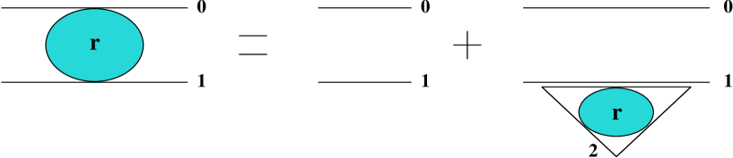
Figure 6: Graphical representation of the evolution equation (32) in the text.

One can immediately see that Eq. (32) is a linearized version of the nonlinear Eq. (43) in [9]. In Fig. 6 the incoming quark $1$ in the dipole splits into a hard gluon $1$ (denoted by a double line on the right hand side of Fig. 6) and into a soft quark $2$. The subsequent evolution continues in the new dipole $12$. In the non-linear evolution equation derived in [9] the evolution could also continue in the original dipole $01$ in the sense of gluon (BK) evolution [15, 16]. However, for an inclusive quantity, such as valence quark production considered here, all further interactions of dipole $01$ cancel by real-virtual cancellations. This is similar to the case of inclusive gluon production cross section considered in [25].

The upper limit of the integral over $\alpha^{\prime}$ (the longitudinal momentum fraction of the soft valence quark at $\underline{z}_{2}$) in Eq. (32) results from two considerations: on the one hand, according to the rules of light-cone perturbation theory [53] $\alpha^{\prime}\leq\alpha_{1}$, while, on the other hand, rapidity ordering of the produced dipoles requires [9]

$$\alpha^{\prime}\,\ll\,\alpha_{1}\,\frac{z_{10}^{2}}{z_{12}^{2}}$$ (33)

as the rapidity of the soft valence quark in dipole $12$ is $y^{\prime}=\ln(\alpha^{\prime}s\,z_{12}^{2})$. (To understand this last formula for $y^{\prime}$ remember that, in transverse momentum space, $y-(Y/2)=\ln(\alpha\,\sqrt{s}/k_{T})$ and $Y=\ln(s/k_{T}^{2})$ leading to $y=\ln(\alpha\,s/k_{T}^{2})$.)

For the dipole-nucleus scattering the effect of harder gluons can be included in the production cross section (31) by

$$\frac{d\sigma^{a}}{d^{2}k\,dy}(\underline{z}_{10},\alpha_{1})\,=\,\frac{1}{(2\pi)^{2}}\frac{\bar{\alpha}_{s}\,N_{c}}{2\pi}\,\frac{\alpha}{\alpha_{1}}\,\int\!d^{2}x\,d^{2}y\,d^{2}z_{1}\,d^{2}z\,e^{i\underline{k}(\underline{x}-\underline{y})}\,r({\underline{z}}_{0},{\underline{z}}_{1},\alpha_{1};\underline{z},\alpha)\,\frac{(\underline{x}-\underline{z})\cdot(\underline{y}-\underline{z})}{|\underline{x}-\underline{z}|^{2}\,|\underline{y}-\underline{z}|^{2}}$$

$$\times\,\left[N(\underline{x},\underline{z})+N(\underline{y},\underline{z})-N(\underline{x},\underline{y})\right],$$ (34)

where we use $y=\ln(\alpha\,s/k_{T}^{2})$ to relate $\alpha$ and $y$.

Inclusion of the evolution effects due to emissions of softer gluon having rapidity less than $y$ is quite straightforward and goes exactly parallel to [25, 26, 57, 58, 59, 60]. To include these softer emissions we need to replace

$$N(\underline{x},\underline{y})\,\rightarrow\,N(\underline{x},\underline{y},y)$$ (35)

in Eq. (34), where now $N(\underline{x},\underline{y},y)$ has to be found from the non-linear evolution equation [15, 16]

$$\frac{\partial N({\underline{x}}_{0},{\underline{x}}_{1},Y)}{\partial Y}\,=\,\frac{\alpha_{s}\,N_{c}}{2\,\pi^{2}}\,\int d^{2}x_{2}\,\frac{x_{01}^{2}}{x_{20}^{2}\,x_{21}^{2}}\,\left[N({\underline{x}}_{0},{\underline{x}}_{2},Y)+N({\underline{x}}_{2},{\underline{x}}_{1},Y)-N({\underline{x}}_{0},{\underline{x}}_{1},Y)\right.$$

$$-\left.N({\underline{x}}_{0},{\underline{x}}_{2},Y)\,N({\underline{x}}_{2},{\underline{x}}_{1},Y)\right]$$ (36)

with the initial condition

$$N({\underline{x}}_{0},{\underline{x}}_{1},Y=0)\,=\,N({\underline{x}}_{0},{\underline{x}}_{1}).$$ (37)

The final answer for the valence quark production cross section including quantum evolution with the valence quark coming from the projectile proton reads

$$\frac{d\sigma^{a}}{d^{2}k\,dy}(\underline{z}_{10},\alpha_{1})\,=\,\frac{1}{(2\pi)^{2}}\frac{\bar{\alpha}_{s}\,N_{c}}{2\pi}\,\frac{\alpha}{\alpha_{1}}\,\int\!d^{2}x\,d^{2}y\,d^{2}z_{1}\,d^{2}z\,e^{i\underline{k}(\underline{x}-\underline{y})}\,r({\underline{z}}_{0},{\underline{z}}_{1},\alpha_{1};\underline{z},\alpha)\,\frac{(\underline{x}-\underline{z})\cdot(\underline{y}-\underline{z})}{|\underline{x}-\underline{z}|^{2}\,|\underline{y}-\underline{z}|^{2}}$$

$$\times\,\left[N(\underline{x},\underline{z},y)+N(\underline{y},\underline{z},y)-N(\underline{x},\underline{y},y)\right].$$ (38)

Once again we remind the reader that here $Y\approx y_{1}=\ln(\alpha_{1}s\,z_{01}^{2})$ and $y=\ln(\alpha\,s/k_{T}^{2})$. When integrating over $\underline{z}$ in Eq. (38) one has to keep in mind that rapidity ordering requires that the rapidity of the quark at transverse coordinate $\underline{z}$, given by ${\tilde{y}}=\ln[\alpha\,s\,(\underline{z}-\underline{z}_{0})^{2}]$, is limited to the interval $y<{\tilde{y}}<Y$, which imposes a constraint on the range of $\underline{z}$-integration.

The essential ingredients of Eq. (38) are the Reggeon exchange amplitude $r$ obeying the evolution equation (32) which sums up leading double logarithms $\alpha_{s}\,\ln^{2}s$, and the amplitude $N$ obeying Eq. (36) summing up usual leading logarithms $\alpha_{s}\,\ln s$. We remind the reader that the fact that we are using the amplitude $r$ obeying a linear evolution equation (32) to describe the evolution between the produced valence quark and the projectile is not an approximation but an exact result of cancellations of non-linear Reggeon evolution corrections from [9] in that rapidity region.

If one is interested only in rapidity dependence of the cross section, integration of Eq. (38) over $k_{T}$ yields

$$\frac{d\sigma^{a}}{dy}(\underline{z}_{10},\alpha_{1})\,=\,\frac{\bar{\alpha}_{s}\,N_{c}}{\pi}\,\frac{\alpha}{\alpha_{1}}\,\int\!d^{2}x\,d^{2}z_{1}\,d^{2}z\,r({\underline{z}}_{0},{\underline{z}}_{1},\alpha_{1};\underline{z},\alpha)\,\frac{1}{|\underline{x}-\underline{z}|^{2}}\,N(\underline{x},\underline{z},y),$$ (39)

where we have also made use of the fact that $N(\underline{x},\underline{x},y)=0$. In the leading double logarithmic approximation we find $\alpha$ from $y\approx\ln(\alpha\,s/Q_{s}^{2}(y))$ where $Q_{s}^{2}(y)$ is the quark saturation scale of the nucleus at rapidity $y$, which we use as the typical transverse momentum of the produced quarks. $Q_{s}^{2}(y)$ is rapidity-dependent due to the effects of nonlinear evolution equation (36).

3.2 Properties of the Cross Section with Evolution

First of all, let us point out that Eq. (32) can be solved analytically if one averages it over the directions of $\underline{z}_{01}$ (or $\underline{z}_{21}$). Defining

$$\underline{\rho}\,\equiv\,\underline{z}-\underline{z}_{0}$$ (40)

we can rewrite Eq. (32) as

$$r({\underline{z}}_{01},\alpha_{1};\underline{\rho},\alpha)\,=\,\delta^{2}(\underline{\rho}-\underline{z}_{10})\,+\,\frac{{\bar{\alpha}}_{s}}{2\,\pi}\,\int_{\alpha}^{\alpha_{1}\,\mbox{min}\{1,z_{01}^{2}/z_{21}^{2}\}}\,\frac{d\alpha^{\prime}}{\alpha^{\prime}}\,\frac{d^{2}z_{2}}{z_{12}^{2}}\,r({\underline{z}}_{21},\alpha^{\prime};\underline{r},\alpha),$$ (41)

which, after angular averaging, becomes

$$r({z}_{01},\alpha_{1};\rho,\alpha)\,=\,\frac{1}{2\,\pi\,\rho}\,\delta(\rho-z_{10})\,+\,\frac{{\bar{\alpha}}_{s}}{2\,\pi}\,\int_{\alpha}^{\alpha_{1}\,\mbox{min}\{1,z_{01}^{2}/z_{21}^{2}\}}\,\frac{d\alpha^{\prime}}{\alpha^{\prime}}\,\frac{d^{2}z_{2}}{z_{12}^{2}}\,r({z}_{21},\alpha^{\prime};r,\alpha).$$ (42)

Similar to [9] we first perform a Mellin transform

$$r({z},\alpha_{1};\rho,\alpha)\,=\,\int\frac{d\omega}{2\pi i}\,\left(\frac{\alpha_{1}\,z^{2}}{\alpha\,\rho^{2}}\right)^{\omega}\,r_{\omega}(z,\rho)$$ (43)

corresponding to Laplace transformation in rapidity. Here the $\omega$-integration runs parallel to the imaginary axis to the right of the origin and, due to rapidity ordering, we use $\alpha_{1}\,z^{2}>\alpha\,\rho^{2}$. Eq. (42) becomes

$$\omega\,r_{\omega}(z_{01},\rho)\,=\,\frac{1}{2\,\pi\,\rho}\,\delta(\rho-z_{01})\,+\,\frac{{\bar{\alpha}}_{s}}{2}\,\int_{0}^{\infty}\,\frac{dz_{21}^{2}}{z_{21}^{2}}\,\left(\mbox{min}\left\{\frac{z_{21}^{2}}{z_{01}^{2}},1\right\}\right)^{\omega}\,r_{\omega}(z_{21},\rho).$$ (44)

We perform another Mellin transformation

$$r_{\omega}(z,\rho)\,=\,\int\,\frac{d\lambda}{2\pi i}\,\left(\frac{\rho^{2}}{z^{2}}\right)^{\lambda}\,r_{\omega\,\lambda}$$ (45)

with the $\lambda$-integration contour being the same as for the $\omega$-integration above and assuming that $z<r$ for all $z_{ij}$’s. We obtain

$$\omega\,r_{\omega\,\lambda}\,=\,\frac{1}{\pi\,\rho^{2}}\,+\,\frac{{\bar{\alpha}}_{s}}{2}\,\frac{\omega}{\lambda\,(\omega-\lambda)}\,r_{\omega\,\lambda}$$ (46)

which gives

$$r_{\omega\,\lambda}\,=\,\frac{1}{\pi\,\rho^{2}}\,\frac{\lambda\,(\omega-\lambda)}{\omega\,[\lambda\,\omega-\lambda^{2}-\frac{{\bar{\alpha}}_{s}}{2}]}.$$ (47)

The solution of Eq. (42) is

$$r({z}_{01},\alpha_{1};\rho,\alpha)\,=\,\frac{1}{\pi\,\rho^{2}}\,\int\frac{d\omega}{2\pi i}\,\frac{d\lambda}{2\pi i}\,\left(\frac{\alpha_{1}\,z_{01}^{2}}{\alpha\,\rho^{2}}\right)^{\omega}\,\left(\frac{\rho^{2}}{z_{01}^{2}}\right)^{\lambda}\,\frac{\lambda\,(\omega-\lambda)}{\omega\,[\lambda\,\omega-\lambda^{2}-\frac{{\bar{\alpha}}_{s}}{2}]}.$$ (48)

Similar to [9] we can first perform the integration over $\omega$ in Eq. (48): arguing that the high-energy asymptotics is dominated by the rightmost pole in $\omega$ plane and picking that pole yields

$$r({z}_{01},\alpha_{1};\rho,\alpha)\,\approx\,\frac{1}{\pi\,\rho^{2}}\,\int\frac{d\lambda}{2\pi i}\,\left(\frac{\alpha_{1}\,z_{01}^{2}}{\alpha\,\rho^{2}}\right)^{\lambda+\frac{{\bar{\alpha}}_{s}}{2\,\lambda}}\,\left(\frac{\rho^{2}}{z_{01}^{2}}\right)^{\lambda}\,\frac{{\bar{\alpha}}_{s}}{2\,\lambda^{2}+{\bar{\alpha}}_{s}}.$$ (49)

Eq. (49) can be evaluated in the saddle point approximation near the saddle point at $\lambda=\sqrt{{\bar{\alpha}}_{s}/2}$, which gives

$$r({z}_{01},\alpha_{1};\rho,\alpha)\,\propto\,\frac{1}{\rho^{2}}\,e^{\sqrt{2\,{\bar{\alpha}}_{s}}\,(y_{1}-y)}\,\left(\frac{\rho^{2}}{z_{01}^{2}}\right)^{\sqrt{\frac{{\bar{\alpha}}_{s}}{2}}}$$ (50)

leading to the well-known intercept of $\sqrt{2\,{\bar{\alpha}}_{s}}$ [19, 20, 21]. A more careful evaluation of Eq. (49) can be done by direct integration. First rewrite Eq. (49) as

$$r({z}_{01},\alpha_{1};\rho,\alpha)\,\approx\,\frac{1}{\pi\,\rho^{2}}\,\int\frac{d\lambda}{2\pi i}\,\left(\frac{\alpha_{1}}{\alpha}\right)^{\lambda}\,\sum_{n=0}^{\infty}\,\frac{1}{n!}\left[\frac{{\bar{\alpha}}_{s}}{2\,\lambda}\,\ln\left(\frac{\alpha_{1}\,z_{01}^{2}}{\alpha\,\rho^{2}}\right)\right]^{n}\,\frac{{\bar{\alpha}}_{s}}{2\,\lambda^{2}+{\bar{\alpha}}_{s}}.$$ (51)

The expression obtained in Eq. (51) has poles at $\lambda=0$ and at $\lambda=\pm i\sqrt{{\bar{\alpha}}_{s}/2}$. From Eq. (49) it is clear that the poles at $\lambda=\pm i\sqrt{{\bar{\alpha}}_{s}/2}$ do not give leading high energy asymptotics. Concentrating on poles at $\lambda=0$ we neglect $2\,\lambda^{2}$ in the $2\,\lambda^{2}+{\bar{\alpha}}_{s}$ denominator of Eq. (51), integrate each or the terms in the series by picking up the pole at $\lambda=0$ and resum back the series obtaining

$$r({z}_{01},\alpha_{1};\rho,\alpha)\,\approx\,\frac{1}{\pi\,\rho^{2}}\,\sqrt{\frac{{\bar{\alpha}}_{s}\,\ln\left(\frac{\alpha_{1}\,z_{01}^{2}}{\alpha\,\rho^{2}}\right)}{2\,\ln\frac{\alpha_{1}}{\alpha}}}\,I_{1}\left(\sqrt{2\,{\bar{\alpha}}_{s}\,\ln\left(\frac{\alpha_{1}\,z_{01}^{2}}{\alpha\,\rho^{2}}\right)\,\ln\frac{\alpha_{1}}{\alpha}}\right).$$ (52)

Now we turn to studying the behavior of the nuclear modification factor under quantum evolution. First we note that the cross section in Eq. (38) can be further simplified assuming transverse translational invariance of the solutions of the non-linear evolution equation for the dipole scattering amplitude, Eq. (36), which can be achieved by considering an infinite and homogeneous nucleus in the transverse plane. Under this assumption the dipole scattering amplitude becomes a function of a single spatial variable, $N(\underline{r},\underline{b},y)\rightarrow N(r,y)$, and, shifting the integration variables in in the following way:

$$\underline{x}-\underline{z}\equiv\underline{v},$$ (53)

$$\underline{y}-\underline{z}\equiv\underline{w},$$ (54)

$$\underline{z}_{1}\equiv\underline{b},$$ (55)

Eq. (38) can be rewritten as

$$\frac{d\sigma^{a}}{d^{2}k\,dy}(\underline{z}_{10},\alpha_{1})\,=\,\frac{1}{(2\pi)^{2}}\frac{\bar{\alpha}_{s}\,N_{c}}{2\pi}\,\frac{\alpha}{\alpha_{1}}\,\int\!d^{2}b\,d^{2}z\,r({\underline{z}}_{0},{\underline{z}}_{1},\alpha_{1};\underline{z},\alpha)\int\!d^{2}v\,d^{2}w\,e^{i\underline{k}(\underline{v}-\underline{w})}\,\,\frac{\underline{v}\cdot\underline{w}}{|\underline{v}|^{2}\,|\underline{w}|^{2}}$$

$$\left[N(|\underline{v}|,y)+N(|\underline{w}|,y)-N(|\underline{v}-\underline{w}|,y)\right].$$ (56)

Noticeably, the integrations over the arguments of the quark probability density $r$ obeying the linear evolution equation (32) and the one over the arguments of the dipole scattering amplitude $N$ decouple. Thus, the linear evolution (32) only introduces to the cross section a rapidity-dependent prefactor, which carries no information at all of the nucleus and is therefore irrelevant for the nuclear modification factor. This prefactor can be calculated using the approximate solution of the reggeon evolution equation given in Eq. (52). The limits of integration are set by the condition $y_{1}-y\geq\ln\frac{\alpha_{1}z_{01}^{2}}{\alpha z^{2}}=y_{1}-{\tilde{y}}\geq 0$, yielding

$$\int\!d^{2}z\,r({\underline{z}}_{0},{\underline{z}}_{1},\alpha_{1};\underline{z},\alpha)=\frac{y_{1}-y}{\ln\frac{\alpha_{1}}{\alpha}}I_{2}\left(\sqrt{2\,{\bar{\alpha}}_{s}\,(y_{1}-y)\,\ln\frac{\alpha_{1}}{\alpha}}\,\right).$$ (57)

Finally, after performing analytically three of the integrals in the Fourier transform, Eq. (56) turns into

$$\frac{d\sigma^{a}}{d^{2}k\,dy}(\underline{z}_{10},\alpha_{1})\,=\,\int\,d^{2}b\,\frac{y_{1}-y}{\ln\frac{\alpha_{1}}{\alpha}}I_{2}\left(\sqrt{2\,{\bar{\alpha}}_{s}\,(y_{1}-y)\,\ln\frac{\alpha_{1}}{\alpha}}\,\right)\,$$

$$\times\,\int_{0}^{\infty}\!\!\!dv\,\left[\frac{2}{k}\,J_{1}(k\,v)-v\,J_{0}(k\,v)\,\ln\frac{1}{v\,\Lambda}\right]\,N(v,y).$$ (58)

We now evaluate the nuclear modification factor $R_{pA}$ at increasing values of rapidity towards the proton fragmentation region, where the contribution to the cross section given in Eq. (58) is the dominant one. The dipole scattering amplitude entering this equation is obtained by numerically solving Eq. (36), with initial conditions given by the classical limit, Eq. (5), with $Q_{sA}^{2}\!=\!1$ GeV² for the nucleus and $Q_{sp}^{2}\!=\!0.1$ GeV² for the proton, and putting $\alpha_{s}\!=\!0.2$. The contribution to the cross section corresponding to the valence quark coming from the nucleus is included using the quasi-classical formula (21) at all values of rapidity. This is a good approximation for forward enough rapidities, where this contribution is vanishingly small anyway. The results for $R_{pA}$ at rapidities $\Delta Y=y-Y/2=0,1,2,3,4$, are shown in Fig. 7.

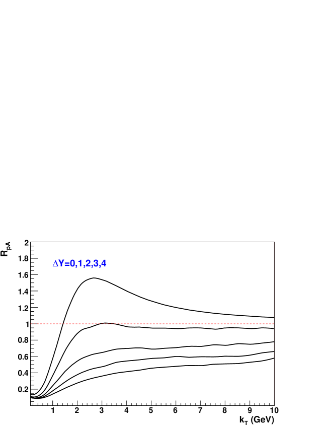
Figure 7: Evolution of $R_{pA}(k_{T},y)$ for valence quarks with rapidity. The initial condition corresponds to $Q_{sA}^{2}=1$ GeV² for a nucleus and $Q_{sp}^{2}=\Lambda^{2}=0.1$ GeV² for a proton. The rapidity interval is measured from mid-rapidity, $\Delta Y=y-Y/2$.

Our results show that the Cronin peak present in the initial condition is wiped out by the evolution, turning into a relative suppression at more forward rapidities. The rate of disappearance of the initial enhancement is similar to the one found in [30] for inclusive gluon production. This is not an unexpected result, since the effects of the reggeon evolution in the $pp$ and $pA$ cross sections are divided out in the nuclear modification factor, whose rapidity dependence is entirely driven by the dipole scattering amplitude, as can be seen from Eq. (58). Moreover, the nuclear modification ratio at large rapidity increases with increasing transverse momentum, and eventually approaches unity at asymptotically large momentum. The slightly irregular behavior of the nuclear modification factor plotted in Fig. 7 at large momentum is due to the numerical uncertainty associated to the Fourier transform in Eq. (58) and has by no means any physical origin.

3.3 Valence Quarks from the Nucleus

Now we want to include quantum evolution corrections into the expression for valence quark production cross section given in Eq. (21), corresponding to the case (b) described above, in which the valence quark originates in the nuclear wave function. As can be seen from Fig. 3, the inclusion of gluon emissions with rapidities greater than the rapidity $y$ of the produced valence quark can be straightforwardly accomplished using the linear dipole (BFKL) evolution, similar to how it was done in [25] for gluon production.

We start by rewriting Eq. (21) for the case of dipole-nucleus scattering, similar to how it was done above in Sect. 3.1 for the case (a):

$$\frac{d\sigma^{b}}{d^{2}k\,dy}(\underline{b}_{01})\,=\,\frac{1}{(2\pi)^{2}}\frac{2\bar{\alpha}_{s}}{\pi}\frac{C_{F}}{1-\frac{C_{F}}{N_{c}}}\frac{e^{-y+Y/2}}{\sqrt{s}|\underline{k}|}\,\int\!d^{2}x\,d^{2}y\,d^{2}B\,e^{i\underline{k}(\underline{x}-\underline{y})}\,\sum_{i,j=0}^{1}\,(-1)^{i+j}\,\frac{(\underline{x}-\underline{b}_{i})\cdot(\underline{y}-\underline{b}_{j})}{|\underline{x}-\underline{b}_{i}|^{2}\,|\underline{y}-\underline{b}_{j}|^{2}}$$

$$\times\,\frac{1}{(\underline{x}-\underline{y})^{2}}\,\left[e^{-(\underline{x}-\underline{y})^{2}Q_{sq}^{2}\ln(1/|\underline{x}-\underline{y}|\Lambda)/4}-e^{-(\underline{x}-\underline{y})^{2}Q_{sg}^{2}\ln(1/|\underline{x}-\underline{y}|\Lambda)/4}\right].$$ (59)

Here $\underline{b}_{0}$ and $\underline{b}_{1}$ are transverse coordinates of the quark and the antiquark in the incoming dipole and $\underline{B}=(1/2)(\underline{b}_{0}+\underline{b}_{1})$ is the transverse coordinate of the center of the dipole. To include the quantum evolution corrections in the rapidity interval between $y$ and $Y$ we first denote the number of dipoles with transverse coordinates ${\underline{b}}_{0^{\prime}},\underline{b}_{1^{\prime}}$ at rapidity $y$ generated by the evolution from the original dipole ${\underline{b}}_{0},\underline{b}_{1}$ having rapidity $Y$ by $n_{1}({\underline{b}}_{0},\underline{b}_{1};{\underline{b}}_{0^{\prime}},\underline{b}_{1^{\prime}};Y-y)$. This quantity is determined from the following evolution equation [14]

$$\frac{\partial n_{1}({\underline{b}}_{0},\underline{b}_{1};{\underline{b}}_{0^{\prime}},\underline{b}_{1^{\prime}};y)}{\partial y}\,=\,\frac{\alpha_{s}\,N_{c}}{2\,\pi^{2}}\,\int d^{2}b_{2}\,\frac{b_{01}^{2}}{b_{20}^{2}\,b_{21}^{2}}\,\bigg{[}n_{1}({\underline{b}}_{0},\underline{b}_{2};{\underline{b}}_{0^{\prime}},\underline{b}_{1^{\prime}};y)+n_{1}({\underline{b}}_{2},\underline{b}_{1};{\underline{b}}_{0^{\prime}},\underline{b}_{1^{\prime}};y)$$

$$-n_{1}({\underline{b}}_{0},\underline{b}_{1};{\underline{b}}_{0^{\prime}},\underline{b}_{1^{\prime}};y)\bigg{]}$$ (60)

with the initial condition

$$n_{1}({\underline{b}}_{0},\underline{b}_{1};{\underline{b}}_{0^{\prime}},\underline{b}_{1^{\prime}};y=0)\,=\,\delta(\underline{b}_{0}-\underline{b}_{0^{\prime}})\,\delta(\underline{b}_{1}-\underline{b}_{1^{\prime}}).$$ (61)

The inclusion of harder gluon emissions is accomplished by the substitution [25]

$$\frac{d\sigma^{b}}{d^{2}k\,dy}(\underline{b}_{01})\,\rightarrow\,\int d^{2}b_{0^{\prime}}\,d^{2}b_{1^{\prime}}\,n_{1}({\underline{b}}_{0},\underline{b}_{1};{\underline{b}}_{0^{\prime}},\underline{b}_{1^{\prime}};Y-y)\,\frac{d\sigma^{b}}{d^{2}k\,dy}(\underline{b}_{0^{\prime}1^{\prime}}).$$ (62)

Inclusion of softer gluon emissions in the rapidity interval between $0$ and $y$ is somewhat more involved. The structure of the quasi-classical result in Eq. (21) crucially depends on the fact that the $t$-channel quark exchanges in Fig. 3 are instantaneous. Attaching a single rung of Reggeon evolution to the quark lines in Fig. 3 would immediately separate the quark lines into a long-lived $s$-channel part and the short-lived $t$-channel part, as shown in Fig. 8. Now the $s$-channel quark line allows for inclusion of quantum evolution corrections as was done in Eq. (32) and in Fig. 6. Thus it is the diagram in Fig. 8 which gets dressed by quantum corrections. The answer for valence quark production cross section will consist of gluon production term given by the diagram in Fig. 3 plus the diagram in Fig. 8, which should be enhanced by quantum corrections. Indeed, the emissions of gluons with rapidities larger than the rapidity $y$ of the produced quark are allowed in Fig. 3 and do not significantly modify its structure. The real difference between Figs. 3 and 8 is due to evolution between the produced quark and the target nucleus, which is allowed only in the latter. In fact, the quasi-classical term from Eq. (21) and Fig. 3 will become negligible compared to Fig. 8 when quantum corrections are included. The situation is similar to the interactions of a current for dilaton-gluon coupling with the nucleus, as was first considered in [55]. Since our expressions here should work for very high energies, we will neglect the contribution of Fig. 3 compared to that of Fig. 8 after quantum evolution is included.

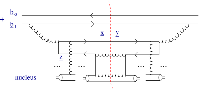
Figure 8: Valence quark production in the case when the valence quark originates in the target nucleus with one rung of small-$x$ evolution included. This diagram in turn serves as a lowest order diagram for the inclusion of small-$x$ evolution corrections discussed in the text.

The calculation of the diagram in Fig. 8 proceeds along the lines of [60]. The wave function squared for an incoming quark at transverse coordinate $\underline{0}$ decaying into a gluon which then decays into a hard massless quark and a soft anti-quark is given by [60]

$${\tilde{\Phi}}(\underline{x},\underline{y};\underline{z},\alpha)\,=\,4\,C_{F}\,\bigg{(}\frac{\alpha_{s}}{\pi}\bigg{)}^{2}\,\frac{\underline{x}\cdot(\underline{x}-\underline{z})\ \underline{y}\cdot(\underline{y}-\underline{z})+\epsilon_{ij}\,x_{i}\,z_{j}\,\epsilon_{kl}\,y_{k}\,z_{l}}{\underline{x}^{2}\,\underline{y}^{2}\,(\underline{x}-\underline{z})^{2}\,(\underline{y}-\underline{z})^{2}}.$$ (63)

The hard quark (to be produced) has transverse coordinates $\underline{x}$ and $\underline{y}$ to the left and to the right of the cut correspondingly, as shown in Fig. 8. A much softer anti-quark has a transverse coordinate $\underline{z}$ and a fraction $\alpha\ll 1$ of the gluon’s longitudinal momentum. Also, $\epsilon_{12}=1$, $\epsilon_{21}=-1$ and $\epsilon_{11}=\epsilon_{22}=0$.

Since the emissions of harder gluons which are described above in the dipole model framework lead to production of a dipole with transverse coordinates which for the moment we will denote by $\underline{b}_{0}$ and $\underline{b}_{1}$ for the quark and for the anti-quark, we rewrite the wave function from Eq. (63) for the case of an incoming dipole (instead of incoming quark) as

$${\tilde{\Phi}}(\underline{x},\underline{y};\underline{z},\alpha)\,\rightarrow\,\sum_{i,j=0}^{1}\,(-1)^{i+j}\,\Phi(\underline{x}-\underline{b}_{i},\underline{y}-\underline{b}_{j};\underline{z},\alpha)$$ (64)

where

$$\Phi(\underline{x}-\underline{b}_{i},\underline{y}-\underline{b}_{j};\underline{z},\alpha)\,=\,4\,C_{F}\,\bigg{(}\frac{\alpha_{s}}{\pi}\bigg{)}^{2}\,\frac{1}{(\underline{x}-\underline{b}_{i})^{2}\,(\underline{y}-\underline{b}_{j})^{2}\,(\underline{x}-\underline{z})^{2}\,(\underline{y}-\underline{z})^{2}}$$

$$\times\,\left[(\underline{x}-\underline{b}_{i})\cdot(\underline{x}-\underline{z})\ (\underline{y}-\underline{b}_{j})\cdot(\underline{y}-\underline{z})+\epsilon_{mn}\,(\underline{x}-\underline{b}_{i})_{m}\,(\underline{x}-\underline{z})_{n}\,\epsilon_{kl}\,(\underline{y}-\underline{b}_{j})_{k}\,(\underline{y}-\underline{z})_{l}\right].$$ (65)

The interaction of the soft quark with transverse coordinate $\underline{z}$ with the nucleus is limited to exchange of two $t$-channel quarks, as shown in Fig. 8. Indeed, since this quark has the same transverse coordinate on both sides of the cut, the multiple rescattering corrections (with gluon exchanges like the ones shown in Figs. 1 and 3) cancel via real-virtual cancellations. The interaction of the quark at $\underline{z}$ with the nucleus is then given by (see Appendix B of [9])

$$r_{int}^{(0)}(\underline{z},\alpha)\,=\,\frac{2\,C_{F}^{2}\,\pi\,\alpha_{s}^{2}}{\alpha\,{\hat{s}}}\,\rho\,T_{A}(\underline{b})\,\ln\frac{\hat{s}}{\Lambda^{2}}$$ (66)

where $\hat{s}=s\,e^{-Y+y}$ is the center-of-mass energy of the incoming gluon-nucleus system in Fig. 8 with $s$ the center-of-mass energy of the whole collision. $\Lambda$ is some infrared cutoff and we took into account the fact that nucleon contains $N_{c}$ valence quarks.

The hard quark having transverse coordinates $\underline{x}$ and $\underline{y}$ in Fig. 8 also can interact with the nucleus. Since the transverse coordinates of the hard quark are different on both sides of the cut ($\underline{x}$ and $\underline{y}$), real-virtual cancellations do not take place, and the interaction of this quark with the target brings in a Glauber-Mueller factor of

$$e^{-(\underline{x}-\underline{y})^{2}Q_{sq}^{2}\ln(1/|\underline{x}-\underline{y}|\Lambda)/4}.$$ (67)

Combining Eqs. (64), (66) and (67) and adjusting the overall normalization similar to how it was done in [60] we write the following expression for the quasi-classical valence quark production cross section in Fig. 8

$$\frac{d\sigma^{b}}{d^{2}k\,dy}(\underline{b}_{01})\,=\,\frac{1}{2\,(2\pi)^{4}}\,\int d^{2}x\,d^{2}y\,d^{2}z\,d^{2}B\,e^{i\underline{k}\cdot(\underline{x}-\underline{y})}\,\int_{0}^{1}d\alpha\,\sum_{i,j=0}^{1}\,\Phi(\underline{x}-\underline{b}_{i},\underline{y}-\underline{b}_{j};\underline{z},\alpha)$$

$$\times\,r_{int}^{(0)}(\underline{z},\alpha)\,e^{-(\underline{x}-\underline{y})^{2}Q_{sq}^{2}\ln(1/|\underline{x}-\underline{y}|\Lambda)/4}.$$ (68)

Eq. (68) makes inclusion of quantum corrections into the diagram of Fig. 8 quite straightforward. The emission of harder gluons is accomplished by the substitution in Eq. (62) as discussed above. All the possible emissions of softer gluons are illustrated in Fig. 9. A gluon may be emitted and absorbed by the harder quark, leading to nonlinear small-$x$ evolution of the quark-anti-quark dipole $\underline{x}$, $\underline{y}$. Similar to [25] such evolution is included in the expression (68) by substituting

$$e^{-(\underline{x}-\underline{y})^{2}Q_{sq}^{2}\ln(1/|\underline{x}-\underline{y}|\Lambda)/4}\,\rightarrow\,1-N(\underline{x},\underline{y},y)$$ (69)

where $N(\underline{x},\underline{y},y)$ is given by the solution of Eq. (36). In making the substitution of Eq. (69) we are including gluon emissions both before and after the interaction with the target [25].

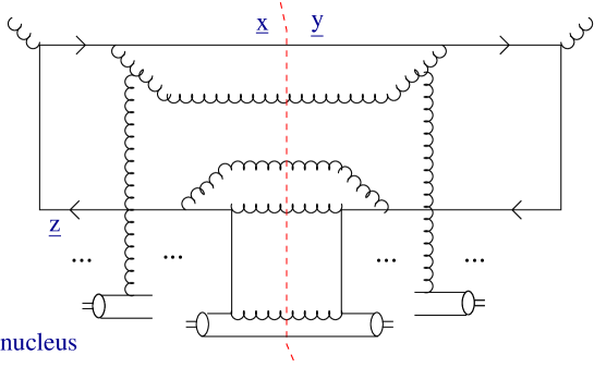
Figure 9: Some examples of quantum evolution corrections to the diagram in Fig. 8: one may have emission and absorption by the hard and soft quark lines, as shown in the figure and discussed in the text.

A gluon may not be emitted by the hard quark at $\underline{x}$ or $\underline{y}$ and absorbed by the soft anti-quark at $\underline{z}$ (and vice versa) because such diagrams are $N_{c}$-suppressed. The only other allowed $s$-channel gluon lines are the emissions and absorptions of the gluon by the soft anti-quark at $\underline{z}$ as is also shown in Fig. 9. The gluon emitted this way can only be emitted before the interaction with the target: late-time emissions cancel by real-virtual cancellations [62]. Since these gluons are emitted before the interaction on both sides of the cut, and as their transverse momenta are integrated over, their interactions with the target nucleus will cancel, just like they did for the anti-quark at $\underline{z}$. The result of such gluon emissions would thus be a linear evolution similar to the one shown in Fig. 6 but with $r_{int}^{(0)}(\underline{z},\alpha)$ from Eq. (66) as the initial condition. The evolution equation reads

$$r_{int}(\underline{x},\underline{y};\underline{z},\alpha)\,=\,r_{int}^{(0)}(\underline{z},\alpha)\,+\,\frac{{\bar{\alpha}}_{s}}{2\,\pi}\,\int_{\alpha_{0}}^{\alpha\,\mbox{min}\left\{1,\frac{(\underline{z}-\underline{x})^{2}}{(\underline{z}-\underline{z}_{2})^{2}},\frac{(\underline{z}-\underline{y})^{2}}{(\underline{z}-\underline{z}_{2})^{2}}\right\}}\,\frac{d\alpha^{\prime}}{\alpha}\,\frac{d^{2}z_{2}}{(\underline{z}-\underline{z}_{2})^{2}}\,r_{int}({\underline{z}},\underline{z};{\underline{z}}_{2},\alpha^{\prime}).$$ (70)

Just like for Eq. (32) the upper limit of $\alpha^{\prime}$-integral is derived by requiring ordering in rapidity. $\alpha_{0}$ is some initial value of $\alpha$ at which the initial conditions are set. In the first step of the evolution in Eq. (70) the ordering in rapidity is imposed by using both distances $|\underline{z}-\underline{x}|$ and $|\underline{z}-\underline{y}|$ as cutoffs, since the hard quark is the one we are tagging on and it has two different transverse coordinates on both sides of the cut. The subsequent steps of the evolution are easier, since there the harder quark will only have one coordinate. The resulting quantity $r_{int}({\underline{w}},\underline{w};{\underline{z}},\alpha)$ obeys the following evolution equation, which is obtained from Eq. (70) by simply putting $\underline{x}=\underline{y}=\underline{w}$:

$$r_{int}(\underline{w},\underline{w};\underline{z},\alpha)\,=\,r_{int}^{(0)}(\underline{z},\alpha)\,+\,\frac{{\bar{\alpha}}_{s}}{2\,\pi}\,\int_{\alpha_{0}}^{\alpha\,\mbox{min}\left\{1,\frac{(\underline{z}-\underline{w})^{2}}{(\underline{z}-\underline{z}_{2})^{2}}\right\}}\,\frac{d\alpha^{\prime}}{\alpha}\,\frac{d^{2}z_{2}}{(\underline{z}-\underline{z}_{2})^{2}}\,r_{int}({\underline{z}},\underline{z};{\underline{z}}_{2},\alpha^{\prime}).$$ (71)

With the help of Eqs. (62), (69) and (70) we write the expression for the valence quark production cross section with the quark originating in the nuclear wave function including the effects of small-$x$ evolution

$$\frac{d\sigma^{b}}{d^{2}k\,dy}(\underline{b}_{01})\,=\,\frac{1}{2\,(2\pi)^{4}}\,\int d^{2}x\,d^{2}y\,d^{2}z\,d^{2}B\,d^{2}b_{0^{\prime}}\,d^{2}b_{1^{\prime}}\,n_{1}({\underline{b}}_{0},\underline{b}_{1};{\underline{b}}_{0^{\prime}},\underline{b}_{1^{\prime}};Y-y)\,e^{i\underline{k}\cdot(\underline{x}-\underline{y})}$$

$$\times\,\int_{0}^{1}d\alpha\,\sum_{i,j=0}^{1}\,\Phi(\underline{x}-\underline{b}_{i^{\prime}},\underline{y}-\underline{b}_{j^{\prime}};\underline{z},\alpha)\,r_{int}(\underline{x},\underline{y};\underline{z},\alpha)\,[1-N(\underline{x},\underline{y},y)].$$ (72)

Integrating Eq. (72) over $k_{T}$ gives the following expression for the rapidity distribution of the stopped baryon number

$$\frac{d\sigma^{b}}{dy}(\underline{b}_{01})\,=\,\frac{1}{2\,(2\pi)^{2}}\,\int d^{2}x\,d^{2}z\,d^{2}B\,d^{2}b_{0^{\prime}}\,d^{2}b_{1^{\prime}}\,n_{1}({\underline{b}}_{0},\underline{b}_{1};{\underline{b}}_{0^{\prime}},\underline{b}_{1^{\prime}};Y-y)$$

$$\times\,\int_{0}^{1}d\alpha\,\sum_{i,j=0}^{1}\,\Phi(\underline{x}-\underline{b}_{i^{\prime}},\underline{x}-\underline{b}_{j^{\prime}};\underline{z},\alpha)\,r_{int}(\underline{x},\underline{x};\underline{z},\alpha).$$ (73)

It is interesting to note that, as could be expected, all the non-linear effects disappeared from $d\sigma^{b}/dy$.

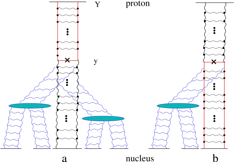
Figure 10: Fan diagrams corresponding to the ’a’ and ’b’ contributions to the valence quark production cross section including the quantum evolution effects given by Eqs. (38) and (72) correspondingly.

The essential ingredients of Eq. (72) are the Reggeon exchange amplitude $r_{int}$ obeying the linear equation (70) summing up powers of $\alpha_{s}\,\ln^{2}s$, and the amplitudes $n_{1}$ and $N$ obeying Eqs. (60) and (36) correspondingly, which sum powers of $\alpha_{s}\,\ln s$. Note that at high $k_{T}$, in the regime where evolution is linear, one can neglect $N$ in Eq. (72), and, keeping only the linear (BFKL) part of Eq. (36) for $N$ in Eq. (38), one can show that each of the equations (38) and (72) become dependent on a convolution of the BFKL pomeron and Reggeon exchange amplitudes.

The fan diagram representation of the valence quark production cross sections calculated in Eqs. (38) and (72) are shown in Fig. 10. The diagram ’a’ in Fig. 10 illustrates a contribution to Eq. (38) with the valence quark originating in the proton: the diagram has a linear Reggeon evolution between the proton and the produced valence quark, with a full non-linear evolution of Eq. (36) represented by fan diagrams between the produced quark and the target nucleus. The diagram ’b’ in Fig. 10 displays a contribution to Eq. (72) with the valence quark originating in the nucleus: it has a linear BFKL evolution between the proton and the produced valence quark, a linear Reggeon evolution between the produced quark and the target, along with a possibility of a non-linear splitting attached to the produced valence quark line.

4 Conclusions

Above we presented calculations of valence quark production far from the fragmentation region in $pA$ collisions. The answers for production cross section in the quasi-classical approximation are given by Eqs. (20) and (21) corresponding to the valence quark originating in the proton and nucleus. The quasi-classical results lead to Cronin-like enhancement of nuclear modification factor for stopped baryons, as shown in Fig. 5. Obtained transverse momentum spectra of the produced valence quarks scale as $\sim 1/k_{T}^{3}$ at high $k_{T}$ and at fixed rapidity, indicating higher sensitivity of quark production to the physics at the ultraviolet end of the spectrum.

Quantum evolution corrections, in the sense of double logarithmic reggeon evolution of [19, 20, 21, 22] and single logarithmic gluon evolution of [15, 16] are included in the valence quark production cross section with the answers given by Eqs. (38) and (72) corresponding to the valence quark originating in the proton and in the nucleus. Eq. (38) contains the effects of double-logarithmic linear reggeon evolution in the rapidity interval between the produced quark and the projectile along with non-linear gluon evolution effects between the quark and the target nucleus. The nuclear modification factor of stopped baryons coming from the projectile proton (due to Eq. (38)) is explored and shown to give suppression of the produced baryons at higher energies and/or rapidities (see Fig. 7). Therefore, based on the valence quark production spectrum and barring the effects of fragmentation functions and of non-perturbative mechanisms of baryon stopping [4, 5, 6, 7, 8], we expect the stopped baryon spectrum to exhibit suppression in the forward rapidity region in $d+Au$ collisions at RHIC. Indeed similar effects should be expected at LHC (possibly even at mid-rapidity [45]) if a $pA$ run is to be conducted there.

Eq. (72) gives us the baryon stopping cross section with the valence quark coming from the nucleus. It includes linear BFKL evolution between the produced quark and the projectile and a combination of linear reggeon evolution and the non-linear evolution from Eq. (36) in the rapidity interval between the quark and the target. The study of the impact of small-$x$ reggeon evolution in Eq. (72) on nuclear modification factor is left for future work. Qualitatively we expect weaker suppression than for baryons coming from the proton, but the onset of this suppression should happen at smaller rapidities. Indeed for the non-linear evolution effects to become important the valence quark should be sufficiently far away in rapidity from the target. Due to the double-logarithmic nature of reggeon evolution one should expect it to manifest itself at smaller rapidities than the gluon evolution. At the same time, as the valence quark production cross section in Eq. (72) falls off approximately as $\sim e^{-y}$, the non-linear evolution effects in it are likely to become important in the rapidity region where baryon stopping in the nucleus (i.e., the cross section itself) is small. This is likely to be the case at RHIC, where the small-$x$ evolution effects do not become important until forward rapidity: there baryon stopping will be dominated by the valence quarks coming from the projectile deuteron (or proton) and baryon stopping due to Eq. (38) will prevail over that from Eq. (72). In other words evolution effects in baryon stopping in the nucleus for $d+A$ collisions at RHIC may become important only in the rapidity region where baryon stopping is dominated by baryons from the deuteron. Therefor, in order to test Eq. (72) one has to perform $pA$ collision experiments at the LHC, where even at mid-rapidity one would expect significant small-$x$ evolution effects [45]. There one may find a window in rapidity (probably close to mid-rapidity but also not too distant from the nuclear fragmentation region) where baryon stopping is dominated by the mechanism given by Eq. (72) with the non-linear evolution effects being important.

The results of our calculations are generally applicable to $pA$ collisions to quantify the amount of purely perturbative baryon stopping. In the high-$p_{T}$ sector, for $p_{T}>Q_{s}$, our results are also applicable to nucleus-nucleus collisions. It is likely, though by no means proven, that the obtained cross sections would provide a qualitatively correct description of the nuclear modification factor for the perturbative initial-state baryon stopping in nucleus-nucleus collisions even at $p_{T}<Q_{s}$. Indeed at rapidity close to the fragmentation region of one of the nuclei in $A+A$ collisions one may argue that the saturation scale of that nucleus ($Q_{s2}$) would be small, much smaller than the saturation scale of the other nucleus ($Q_{s1}$), making the particle production processes describable in the framework of $pA$ collisions for a wide range of transverse momenta $p_{T}>Q_{s2}$. Therefore in that rapidity region baryon stopping can be described by the Eq. (38) above. The amount of baryon stopping not far from the fragmentation region is large, allowing for an easy experimental verification of our results.

We conclude by reiterating that suppression of high-$p_{T}$ net baryons in $p(d)+A$ collisions at forward rapidity at RHIC, as predicted above, would provide an independent test of the physics of Color Glass Condensate. (Non-perturbative baryon stopping mechanisms are not likely to be important at high-$p_{T}$.) Similar experiments can be carried out at the LHC. The proposed test of CGC at RHIC with valence quarks may not be as clean as electromagnetic probes [63], which are free from uncertainties introduced by fragmentation functions, but it has the advantage of being possible to perform by analyzing the current experimental data generated at RHIC.

Appendix A

In this Appendix we derive the small-x quark and gluon wavefunction of a fast quark moving in the light cone “plus” direction. The corresponding diagram is shown in Fig. 11. At lowest order in perturbation theory it is given by [53]

$$\psi^{{}^{\prime}a}_{\sigma,\sigma^{\prime}\lambda}(\underline{p},\underline{k},\alpha)=\frac{\langle f|H_{I}|i\rangle/\sqrt{k^{+}p^{+}}}{\sum_{f}p_{f}^{-}-\sum_{i}p_{i}^{-}},$$ (A1)

where $p$ and $\sigma$ are the momentum and helicity of the incoming quark, $k$ and $\sigma^{\prime}$ those of outgoing quark and $a$ and $\lambda$ the color and polarization of the emitted gluon. The transition matrix element is given by

$$\langle f|H_{I}|i\rangle/\sqrt{p^{+}k^{+}}\,=\,g\,t^{a}\frac{\bar{u}_{\sigma}(k)}{\sqrt{k^{+}}}\gamma\cdot\epsilon^{\lambda}(p-k)\frac{u_{\sigma^{\prime}}(p)}{\sqrt{p^{+}}},$$ (A2)

where the gluon polarization vector in in the $A^{+}=0$ gauge is $\epsilon(q)=(0,\frac{2q\cdot\epsilon^{\lambda}}{q^{+}},\underline{\epsilon}^{\lambda})$ with $\underline{\epsilon}^{\lambda}=\frac{1}{\sqrt{2}}(1,i\lambda)$ and $\lambda=\pm 1$.

Figure 11: Diagram for soft quark wavefunction calculation.

Defining $\alpha=k^{+}/p^{+}$, the energy denominator is

$$\Sigma_{f}p_{f}^{-}-\Sigma_{i}p_{i}^{-}=-\frac{1}{p^{+}\alpha(1-\alpha)}(\alpha\underline{p}-\underline{k})^{2}$$ (A3)

We note that [53]

$$\frac{\bar{u}_{\sigma}(k)}{\sqrt{k^{+}}}\gamma^{+}\,\frac{u_{\sigma^{\prime}}(p)}{\sqrt{p^{+}}}=2\delta^{\sigma\sigma^{\prime}}$$ (A4)

and

$$\frac{\bar{u}_{\sigma}(k)}{\sqrt{k^{+}}}\gamma^{j}\frac{u_{\sigma^{\prime}}(p)}{\sqrt{p^{+}}}=\left[\frac{k^{j}-i\sigma\epsilon^{jl}k^{l}}{k^{+}}+\frac{p^{j}+i\sigma\epsilon^{jl}p^{l}}{p^{+}}\right]\delta^{\sigma\sigma^{\prime}}$$ (A5)

where $\epsilon^{jl}$ the totally antisymmetric tensor in two dimensions. Using $i\sigma\underline{k}^{l}\epsilon^{jl}\underline{\epsilon}^{\lambda}_{j}=\sigma\lambda\underline{k}\cdot\underline{\epsilon}^{\lambda}$ one immediately gets

$$\psi^{{}^{\prime}a}_{\sigma,\sigma^{\prime}\lambda}(\underline{p},\underline{k},\alpha)=gt^{a}[1+\alpha-(1-\alpha)\sigma\lambda]\frac{(\underline{k}-x\underline{p})\cdot\underline{\epsilon}^{\lambda}}{(\underline{k}-x\underline{p})^{2}}\delta^{\sigma\sigma^{\prime}}.$$ (A6)

Denoting by $\underline{x}_{1}$ the transverse coordinate of the incoming quark and by $\underline{x}_{2}$ and $\underline{x}_{3}$ the transverse coordinates of the outgoing quark and gluon respectively and Fourier-transforming to coordinate space one gets

$$\psi^{{}^{\prime}a}_{\sigma,\sigma^{\prime}\lambda}(\underline{x}_{31},\underline{x}_{23},\alpha)=gt^{a}[1+\alpha-(1-\alpha)\sigma\lambda]\frac{i}{2\pi}\delta(\underline{x}_{31}+\alpha\,\underline{x}_{23})\frac{\underline{x}_{23}\cdot\underline{\epsilon}^{\lambda}}{\underline{x}^{2}_{23}}\delta^{\sigma\sigma^{\prime}}.$$ (A7)

Taking the limit $\alpha\rightarrow 0$ and integrating over the transverse position of the hard gluon sets $\underline{x}_{3}=\underline{x}_{1}$ due to the delta-function and yields

$$\psi^{a}_{\sigma,\sigma^{\prime}\lambda}(\underline{x}_{21},\alpha)=\int d^{2}x_{3}\psi^{{}^{\prime}a}_{\sigma,\sigma^{\prime}\lambda}(\underline{x}_{31},\underline{x}_{23},\alpha)=gt^{a}[1-\sigma\lambda]\frac{i}{2\pi}\frac{\underline{x}_{21}\cdot\underline{\epsilon}^{\lambda}}{\underline{x}^{2}_{21}}\delta^{\sigma\sigma^{\prime}}.$$ (A8)

To define the small-$\alpha$ quark distribution function of a nucleon we multiply the previous wavefunction by its complex conjugate evaluated at different transverse position of the soft quark, average over the helicity of the initial quark and sum over the polarizations and colors of the gluon and integrate over the position of the initial quark ($\underline{x}_{1}$) obtaining

$$\frac{dn^{q}}{d^{2}z\,dy}=\frac{1}{4\pi}\frac{\alpha}{2}\sum_{\sigma,\lambda,a}\langle\psi^{a}_{\sigma,\lambda}(\underline{x}-\underline{z},\alpha)\psi^{*a}_{\sigma,\lambda}(\underline{y}-\underline{z},\alpha)\rangle=\frac{\bar{\alpha}_{s}\,\alpha}{2\pi}\frac{(\underline{x}-\underline{z})\cdot(\underline{y}-\underline{z})}{(\underline{x}-\underline{z})^{2}(\underline{y}-\underline{z})^{2}},$$ (A9)

as given in Eq. (3). The factor $\alpha/2$ arises from the integration over the phase space of the gluon: $d\alpha/2(1-\alpha)\approx\alpha dy/2$.

Taking the limit $1-\alpha\rightarrow 0$ in Eq. (A7) and proceeding analogously one derives the soft gluon distribution function of a valence quark

$$A^{a}_{\sigma,\sigma^{\prime}\lambda}(\underline{x}_{31},\alpha)=\,2\,g\,t^{a}\,\frac{i}{2\pi}\frac{\underline{x}_{31}\cdot\underline{\epsilon}^{\lambda}}{\underline{x}^{2}_{31}}\delta^{\sigma\sigma^{\prime}}\,$$ (A10)

and

$$\frac{dn^{g}}{d^{2}z\,dy}=\frac{1}{4\pi}\,\frac{1}{2}\,\sum_{\sigma,\lambda,a}\langle A^{a}_{\sigma,\lambda}(\underline{x}-\underline{z},\alpha)A^{*a}_{\sigma,\lambda}(\underline{y}-\underline{z},\alpha)\rangle=\frac{\bar{\alpha}_{s}}{\pi}\frac{(\underline{x}-\underline{z})\cdot(\underline{y}-\underline{z})}{(\underline{x}-\underline{z})^{2}(\underline{y}-\underline{z})^{2}}.$$ (A11)

Appendix B

In this appendix we derive the $Gq\rightarrow qG$ scattering cross section in the high energy limit. The calculation is performed in the $A^{+}=0$ gauge, with gluon polarization vectors taken in the same gauge $\epsilon^{+}=0$. The amplitude for the process is shown in Fig. 12 and is equal to

$$M=\bar{u}_{\sigma^{\prime}}(k+l)(igt^{a}\gamma^{\mu})\frac{i\not{l}}{l^{2}+i\epsilon}(igt^{b}\gamma^{\nu})u_{\sigma}(p)\epsilon_{\mu}^{\lambda}(k)\epsilon_{\nu}^{*\lambda^{\prime}}(p-l).$$ (B1)

Squaring the amplitude, averaging over the helicity of the incoming quark and the polarization of the incoming gluon and summing for all possible helicities, polarizations and colors in the final state, one gets

$$\left\langle|M|^{2}\right\rangle\,\equiv\,\frac{1}{4}\,\frac{1}{N(N^{2}-1)}\sum_{a,b,\sigma,\sigma^{\prime},\lambda,\lambda^{\prime}}|M|^{2}\\ =(2\pi)^{2}\frac{C_{F}}{2N_{c}}\frac{\alpha_{s}^{2}}{(l^{2}+i\epsilon)^{2}}\mbox{tr}[(\not{k}+\not{l})\gamma^{\mu}\not{l}\gamma^{\nu}\not{p}\gamma^{\beta}\not{l}\gamma^{\alpha}]d_{\mu\alpha}(k)d_{\nu\beta}(p-l)$$ (B2)

where $d_{\mu\alpha}(k)=\sum_{\lambda}\epsilon_{\mu}^{\lambda}(k)\epsilon_{\alpha}^{*\lambda}(k)=-g_{\mu\alpha}+\frac{k_{\alpha}\eta_{\mu}+k_{\mu}\eta_{\alpha}}{k\cdot\eta}$ is the gluon polarization sum in the light cone gauge.

Figure 12: Gq$\rightarrow$qG scattering amplitude.

Keeping only the leading terms, i.e. those proportional to the center mass energy of the collision, $s=2p^{-}k^{+}$, and putting $l^{2}\approx-\underline{l}^{2}$, we get

$$\left\langle|M|^{2}\right\rangle=4(2\pi)^{2}\frac{\alpha_{s}^{2}C_{F}}{N_{c}}\frac{s}{\underline{l}^{2}}\;.$$ (B3)

Finally, dividing by the flux factor and integrating over the phase space of the produced quark and gluon one gets the final result

$$\sigma^{Gq\rightarrow qG}\,=\,\frac{\alpha_{s}^{2}C_{F}}{N_{c}}\,\frac{1}{s}\int\!\frac{d^{2}\underline{l}}{\underline{l}^{2}}\;.$$ (B4)

References

- [1] H. Appelshauser et al. [NA49 Collaboration], Phys. Rev. Lett. 82, 2471 (1999) [arXiv:nucl-ex/9810014].
- [2] T. Alber et al. [NA35 Collaboration.], Z. Phys. C 64, 195 (1994); T. Alber et al. [NA35 Collaboration], Eur. Phys. J. C 2, 643 (1998) [arXiv:hep-ex/9711001].
- [3] I. G. Bearden et al. [BRAHMS Collaboration], Phys. Rev. Lett. 93, 102301 (2004) [arXiv:nucl-ex/0312023].
- [4] G. Veneziano, Nucl. Phys. B 74, 365 (1974); G. Veneziano, Phys. Lett. B 52, 220 (1974).
- [5] G. C. Rossi and G. Veneziano, Nucl. Phys. B 123, 507 (1977).
- [6] B. Z. Kopeliovich and B. G. Zakharov, Z. Phys. C 43, 241 (1989).
- [7] D. Kharzeev, Phys. Lett. B 378, 238 (1996) [arXiv:nucl-th/9602027].
- [8] A. Capella and C. A. Salgado, Phys. Rev. C 60, 054906 (1999) [arXiv:hep-ph/9903414].
- [9] K. Itakura, Y. V. Kovchegov, L. McLerran and D. Teaney, Nucl. Phys. A 730, 160 (2004) [arXiv:hep-ph/0305332].
- [10] L. V. Gribov, E. M. Levin and M. G. Ryskin, Phys. Rept. 100, 1 (1983); A. H. Mueller and J. w. Qiu, Nucl. Phys. B 268, 427 (1986).
- [11] L. D. McLerran and R. Venugopalan, Phys. Rev. D 49, 2233 (1994) [arXiv:hep-ph/9309289]; Phys. Rev. D 49, 3352 (1994) [arXiv:hep-ph/9311205]; Phys. Rev. D 50, 2225 (1994)
- [12] Y. V. Kovchegov, Phys. Rev. D 54, 5463 (1996) [arXiv:hep-ph/9605446]; Phys. Rev. D 55, 5445 (1997) [arXiv:hep-ph/9701229].
- [13] J. Jalilian-Marian, A. Kovner, L. D. McLerran and H. Weigert, Phys. Rev. D 55, 5414 (1997) [arXiv:hep-ph/9606337].
- [14] A. H. Mueller, Nucl. Phys. B 415, 373 (1994); A. H. Mueller and B. Patel, Nucl. Phys. B 425, 471 (1994) [arXiv:hep-ph/9403256]; A. H. Mueller, Nucl. Phys. B 437, 107 (1995) [arXiv:hep-ph/9408245].
- [15] Y. V. Kovchegov, Phys. Rev. D 60, 034008 (1999) [arXiv:hep-ph/9901281]; Phys. Rev. D 61, 074018 (2000) [arXiv:hep-ph/9905214].
- [16] I. Balitsky, Nucl. Phys. B 463, 99 (1996) [arXiv:hep-ph/9509348]; arXiv:hep-ph/9706411; Phys. Rev. D 60, 014020 (1999) [arXiv:hep-ph/9812311].
- [17] J. Jalilian-Marian, A. Kovner, A. Leonidov and H. Weigert, Nucl. Phys. B 504, 415 (1997) [arXiv:hep-ph/9701284]; Phys. Rev. D 59, 014014 (1999) [arXiv:hep-ph/9706377]; Phys. Rev. D 59, 034007 (1999) [Erratum-ibid. D 59, 099903 (1999)] [arXiv:hep-ph/9807462]; J. Jalilian-Marian, A. Kovner and H. Weigert, Phys. Rev. D 59, 014015 (1999) [arXiv:hep-ph/9709432]; A. Kovner, J. G. Milhano and H. Weigert, Phys. Rev. D 62, 114005 (2000) [arXiv:hep-ph/0004014]; H. Weigert, Nucl. Phys. A 703, 823 (2002) [arXiv:hep-ph/0004044].
- [18] E. Iancu, A. Leonidov and L. D. McLerran, Nucl. Phys. A 692, 583 (2001) [arXiv:hep-ph/0011241]; Phys. Lett. B 510, 133 (2001) [arXiv:hep-ph/0102009]; E. Iancu and L. D. McLerran, Phys. Lett. B 510, 145 (2001) [arXiv:hep-ph/0103032]; E. Ferreiro, E. Iancu, A. Leonidov and L. McLerran, Nucl. Phys. A 703, 489 (2002) [arXiv:hep-ph/0109115].
- [19] R. Kirschner and L. N. Lipatov, Nucl. Phys. B 213, 122 (1983).
- [20] R. Kirschner, Z. Phys. C 31, 135 (1986).
- [21] R. Kirschner, Z. Phys. C 67, 459 (1995) [arXiv:hep-th/9404158]; R. Kirschner, Z. Phys. C 65, 505 (1995) [arXiv:hep-th/9407085].
- [22] S. Griffiths and D. A. Ross, Eur. Phys. J. C 12, 277 (2000) [arXiv:hep-ph/9906550].
- [23] E. A. Kuraev, L. N. Lipatov and V. S. Fadin, Sov. Phys. JETP 45, 199 (1977) [Zh. Eksp. Teor. Fiz. 72, 377 (1977)]; I. I. Balitsky and L. N. Lipatov, Sov. J. Nucl. Phys. 28, 822 (1978) [Yad. Fiz. 28, 1597 (1978)].
- [24] Y. V. Kovchegov and A. H. Mueller, Nucl. Phys. B 529, 451 (1998) [arXiv:hep-ph/9802440].
- [25] Y. V. Kovchegov and K. Tuchin, Phys. Rev. D 65, 074026 (2002) [arXiv:hep-ph/0111362].
- [26] J. Jalilian-Marian and Y. V. Kovchegov, Prog. Part. Nucl. Phys. 56, 104 (2006) [arXiv:hep-ph/0505052].
- [27] A. Dumitru and L. D. McLerran, Nucl. Phys. A 700, 492 (2002) [arXiv:hep-ph/0105268].
- [28] A. Dumitru and J. Jalilian-Marian, Phys. Rev. Lett. 89, 022301 (2002) [arXiv:hep-ph/0204028].
- [29] D. Kharzeev, Y. V. Kovchegov and K. Tuchin, Phys. Rev. D 68, 094013 (2003) [arXiv:hep-ph/0307037].
- [30] J. L. Albacete, N. Armesto, A. Kovner, C. A. Salgado and U. A. Wiedemann, Phys. Rev. Lett. 92, 082001 (2004) [arXiv:hep-ph/0307179].
- [31] R. Baier, A. Kovner and U. A. Wiedemann, Phys. Rev. D 68, 054009 (2003) [arXiv:hep-ph/0305265].
- [32] B. Z. Kopeliovich, A. V. Tarasov and A. Schafer, Phys. Rev. C 59, 1609 (1999) [arXiv:hep-ph/9808378].
- [33] B. Z. Kopeliovich, J. Nemchik, A. Schafer and A. V. Tarasov, Phys. Rev. Lett. 88, 232303 (2002) [arXiv:hep-ph/0201010].
- [34] X. N. Wang, Phys. Rev. Lett. 81 (1998) 2655; M. Gyulassy and P. Levai, Phys. Lett. B 442 (1998) 1; X. N. Wang, Phys. Rev. C 61 (2000) 064910.
- [35] E. Wang and X. N. Wang, Phys. Rev. C 64 (2001) 034901; Y. Zhang, G. Fai, G. Papp, G. G. Barnafoldi and P. Levai, Phys. Rev. C 65 (2002) 034903; I. Vitev and M. Gyulassy, Phys. Rev. Lett. 89 (2002) 252301.
- [36] I. Vitev, Phys. Lett. B 562, 36 (2003); [arXiv:nucl-th/0302002].
- [37] X. N. Wang, Phys. Lett. B 565 (2003) 116; X. N. Wang, arXiv:nucl-th/0305010; X. Zhang and G. Fai, arXiv:hep-ph/0306227. G. G. Barnafoldi, G. Papp, P. Levai and G. Fai, arXiv:nucl-th/0307062.
- [38] J. W. Cronin, H. J. Frisch, M. J. Shochet, J. P. Boymond, R. Mermod, P. A. Piroue and R. L. Sumner, Phys. Rev. D 11, 3105 (1975).
- [39] D. Kharzeev, E. Levin and L. McLerran, Phys. Lett. B 561, 93 (2003) [arXiv:hep-ph/0210332].
- [40] R. Debbe, [BRAHMS Collaboration], talk given at the APS DNP Meeting at Tucson, AZ, October, 2003; R. Debbe [BRAHMS Collaboration], arXiv:nucl-ex/0403052.
- [41] I. Arsene et al. [BRAHMS Collaboration], Phys. Rev. Lett. 93, 242303 (2004) [arXiv:nucl-ex/0403005].
- [42] B. B. Back et al. [PHOBOS Collaboration], Phys. Rev. C 70, 061901 (2004) [arXiv:nucl-ex/0406017].
- [43] S. S. Adler et al. [PHENIX Collaboration], Phys. Rev. Lett. 94, 082302 (2005) [arXiv:nucl-ex/0411054].
- [44] G. Rakness [STAR Collaboration], talks given at XXXXth Rencontres de Moriond, “QCD and Hadronic Interactions at High Energy”, March 12-19, 2005, La Thuile, Italy and at the XIII International Workshop on Deep Inelastic Scattering (DIS2005), April 27 - May 1, 2005, Madison, Wisconsin, USA; see also L. S. Barnby [STAR Collaboration], [arXiv:nucl-ex/0404027].
- [45] D. Kharzeev, Y. V. Kovchegov and K. Tuchin, Phys. Lett. B 599, 23 (2004) [arXiv:hep-ph/0405045].
- [46] J. Jalilian-Marian, Nucl. Phys. A 748, 664 (2005) [arXiv:nucl-th/0402080].
- [47] A. Dumitru, A. Hayashigaki and J. Jalilian-Marian, Nucl. Phys. A 765, 464 (2006) [arXiv:hep-ph/0506308]; Nucl. Phys. A 770, 57 (2006) [arXiv:hep-ph/0512129].
- [48] A. Dumitru, L. Gerland and M. Strikman, Phys. Rev. Lett. 90, 092301 (2003) [Erratum-ibid. 91, 259901 (2003)] [arXiv:hep-ph/0211324]; A. Berera, M. Strikman, W. S. Toothacker, W. D. Walker and J. J. Whitmore, “The Limiting Curve of Leading Particles from Hadron-Nucleus Collisions at Phys. Lett. B 403, 1 (1997) [arXiv:hep-ph/9604299]; L. Frankfurt and M. Strikman, “The STAR forward pion production in d Au collisions and dynamics of arXiv:nucl-th/0603049.
- [49] R. Cutler and D. W. Sivers, Phys. Rev. D 17, 196 (1978).
- [50] Y. V. Kovchegov and A. H. Mueller, Phys. Lett. B 439, 428 (1998) [arXiv:hep-ph/9805208].
- [51] Y. V. Kovchegov, Nucl. Phys. A 692, 557 (2001) [arXiv:hep-ph/0011252].
- [52] R. Baier, Y. L. Dokshitzer, A. H. Mueller, S. Peigne and D. Schiff, Nucl. Phys. B 484, 265 (1997) [arXiv:hep-ph/9608322].
- [53] G. P. Lepage and S. J. Brodsky, Phys. Rev. D 22, 2157 (1980).
- [54] A. H. Mueller, Phys. Rev. D 2, 2963 (1970).
- [55] A. H. Mueller, Nucl. Phys. B 335, 115 (1990).
- [56] I. Arsene et al. [BRAHMS Collaboration], Phys. Rev. Lett. 91, 072305 (2003) [arXiv:nucl-ex/0307003].
- [57] J. Jalilian-Marian and Y. V. Kovchegov, Phys. Rev. D 70, 114017 (2004) [Erratum-ibid. D 71, 079901 (2005)] [arXiv:hep-ph/0405266].
- [58] C. Marquet, Nucl. Phys. B 705, 319 (2005) [arXiv:hep-ph/0409023].
- [59] Y. V. Kovchegov, Phys. Rev. D 72, 094009 (2005) [arXiv:hep-ph/0508276].
- [60] Y. V. Kovchegov and K. Tuchin, arXiv:hep-ph/0603055.
- [61] N. N. Nikolaev and B. G. Zakharov, Z. Phys. C 49, 607 (1991).
- [62] Z. Chen and A. H. Mueller, Nucl. Phys. B 451, 579 (1995).
- [63] F. Gelis and J. Jalilian-Marian, Phys. Rev. D 66, 014021 (2002) [arXiv:hep-ph/0205037]; Phys. Rev. D 66, 094014 (2002) [arXiv:hep-ph/0208141]; R. Baier, A. H. Mueller and D. Schiff, Nucl. Phys. A 741, 358 (2004) [arXiv:hep-ph/0403201]; J. Jalilian-Marian, arXiv:hep-ph/0501222; Nucl. Phys. A 739, 319 (2004) [arXiv:nucl-th/0402014]; M. A. Betemps and M. B. Gay Ducati, Phys. Rev. D 70, 116005 (2004) [arXiv:hep-ph/0408097].