Abstract

The complementarity between the quark and lepton mixing matrices is shown to provide a robust prediction for the neutrino mixing angle $\theta_{13}^{PMNS}$. We obtain this prediction by first showing that the matrix $V_{M}$, product of the CKM and PMNS mixing matrices, may have a zero (1,3) entry which is favored by experimental data. Hence models with bimaximal or tribimaximal forms of the correlation matrix $V_{M}$ are quite possible. Any theoretical model with a vanishing (1,3) entry of $V_{M}$ that is in agreement with quark data, solar, and atmospheric mixing angle leads to $\theta_{13}^{PMNS}=(9{{}^{+1}_{-2}})^{\circ}$. This value is consistent with the present 90% CL experimental upper limit.

PACS: 14.60.Pq, 14.60.Lm, 96.40.Tv.

$\star$ chauhan@cftp.ist.utl.pt, Marco.Picariello@cern.ch, pulido@cftp.ist.utl.pt, torrente@cern.ch

1 Introduction

Recent neutrino experiments confirm that the Pontecorvo-Maki-Nakagawa-Sakata (PMNS) [1, 2] lepton mixing matrix $U_{PMNS}$ contains large mixing angles. For example the atmospheric mixing $\theta_{23}^{PMNS}$ is compatible with $45^{\circ}$ [3], and the solar mixing $\theta_{12}^{PMNS}$ is $\approx 34^{\circ}$ [4]. These results should be compared with the third lepton mixing angle $\theta_{13}^{PMNS}$ which is very small and even compatible with zero [5, 6], and with the quark mixing angles in the $U_{CKM}$ matrix [7, 8].

The disparity that nature indicates between quark and lepton mixing angles has been viewed in terms of a ’quark-lepton complementarity’ (QLC) [9] which can be expressed in the relations

$$\theta_{12}^{PMNS}+\theta_{12}^{CKM}\simeq 45^{\circ}\,;\quad\quad\theta_{23}^{PMNS}+\theta_{23}^{CKM}\simeq 45^{\circ}\,.$$ (1)

Possible consequences of QLC have been investigated in the literature [10] and in particular a simple correspondence between the $U_{PMNS}$ and $U_{CKM}$ matrices has been proposed [9, 11, 12, 13] and analyzed in terms of a correlation matrix [14, 15, 16, 17, 18, 19, 20]. The correlation matrix $V_{M}$ is simply defined as the product of the CKM and PMNS matrices, $V_{M}=U_{CKM}\cdot U_{PMNS}$, and efforts have been done to obtain the most favorite pattern for the matrix $V_{M}$ [20, 21]. Unitarity then implies $U_{PMNS}=U^{\dagger}_{CKM}V_{M}$ and one may ask where do the large lepton mixings come from? Is this information implicit in the form of the $V_{M}$ matrix? This question has been widely investigated in the literature, but its answer is still open (see our section 2).

Furthermore in some Grand Unification Theories (GUTs) the direct QLC correlation between the $CKM$ and the $PMNS$ mixing matrix can be obtained. In this class of models, the $V_{M}$ matrix is determined by the heavy Majorana neutrino mass matrix [12, 22]. Moreover as long as quarks and leptons are inserted in the same representation of the underlying gauge group, we need to include in our definition of $V_{M}$ arbitrary but non trivial phases between the quark and lepton matrices. Hence we will generalize the relation $V_{M}=U_{CKM}\cdot U_{PMNS}$ to

$$V_{M}=U_{CKM}\cdot\Omega\cdot U_{PMNS}\,$$ (2)

where the quantity $\Omega$ is a diagonal matrix $\Omega={\rm diag}(e^{{\rm i}\omega_{i}})$ and the three phases $\omega_{i}$ are free parameters (in the sense that they are not restricted by present experimental evidence).

The magnitude disparity between the lepton mixing angle $\theta_{13}^{PMNS}$ and the other two mixings is a rather striking fact. In this paper we carry out the investigation of the correlation matrix $V_{M}$ based on eq. (2) and prove that it is a zero texture of $V_{M}$, namely $V_{M_{13}}=0$, that implies a small value for $\theta_{13}^{PMNS}$ with a sharp prediction

$$\theta_{13}^{PMNS}=(9\pm^{1}_{2})^{\circ}.$$ (3)

We use the Wolfenstein parameterization for $U_{CKM}$ [23] in its unitary form [24] and parameterize $U_{PMNS}$ with the standard phases and mixing angles. As a zero order approximation we start inserting by hand the central values of the lepton mixing angles and CKM parameters. Owing to the uncertainty in the experimental value for $\theta_{13}^{PMNS}$, the possible range for the (1,3) entry of matrix $V_{M}$ may or may not include zero. For example using $\theta_{13}^{PMNS}=3^{\circ}$ the (1,3) entry range does not include zero in accordance with eq. (23) in ref. [14]. For other choices of $\theta_{13}^{PMNS}$ a vanishing (1,3) entry is quite possible, as will be seen in section 2.

It is possible to include bimaximal and tribimaximal forms of the correlation matrix $V_{M}$ in models with renormalization effects [25, 26, 27] that are relevant, however, only in particular cases with large $\tan\beta$ $(>40)$ and with quasi degenerate neutrino masses [28]. The conclusion for matrix $V_{M}$ is that the possibility of a bimaximal form, or a tribimaximal one is completely open. So in other words, the correlation between the matrices $U_{CKM}$ and $U_{PMNS}$ is rather nontrivial.

The investigation we perform for the $V_{M}$ matrix starts from the fundamental equation $V_{M}=U_{CKM}\cdot\Omega\cdot U_{PMNS}$ and uses the experimental ranges and constraints on lepton mixing angles. We resort to a Monte Carlo simulation with two-sided Gaussian distributions around the mean values of the observables. The input information on $\theta_{13}^{PMNS}$ is taken from the analysis of ref. [3] which uses neutrino data only.

The paper is organized as follows: in section 2 we study the numerical ranges of $V_{M}$ entries with the aid of a Monte Carlo simulation, emphasizing on specific points of the experimental data. We will show that the vanishing of the $(1,3)$ entry is favored by the data analysis. In section 3 we present the matter from a different point of view: we start from a zero $(1,3)$ $V_{M}$ entry (e.g. a bimaximal or tribimaximal matrix) we derive the consequent prediction for the $U_{PMNS}$ lepton mixing matrix through

$$U_{PMNS}=(U_{CKM}\cdot\Omega)^{-1}\cdot V_{M}$$ (4)

and the corresponding one for $\theta_{13}^{PMNS}$ in eq. (3). Finally we present a summary and our conclusions.

2 Which $V_{M}$ does the phenomenology imply?

In this section we investigate the order of magnitude of the $V_{M}$ matrix entries concentrating in particular in the (1,3) entry and the important mixing angle $\theta_{13}^{V_{M}}$ to which it is directly related. We then explicitly study the allowed values of the $V_{M}$ angles, finally concluding that $sin^{2}\theta_{13}^{V_{M}}=0$ is the value most favored by the data. We will be using the Wolfenstein parameterization [23] of the $U_{CKM}$ matrix in its unitary form [24] where one has the relation

$$\sin\theta_{12}^{CKM}=\lambda\quad\quad\sin\theta_{23}^{CKM}=A\lambda^{2}\quad\quad\sin\theta_{13}^{CKM}e^{-{\rm i}\delta^{CKM}}=A\lambda^{3}(\rho-{\rm i}\eta)$$ (5)

to all orders in $\lambda$. The lepton mixing matrix $U_{PMNS}$ is parameterized in the usual way as

$$U_{PMNS}=U_{23}\cdot\Phi\cdot U_{13}\cdot\Phi^{\dagger}\cdot U_{12}\cdot\Phi_{m}.$$ (6)

Here $\Phi$ and $\Phi_{m}$ are diagonal matrices containing the Dirac and Majorana CP violating phases, respectively $\Phi={\rm diag}(1,1,e^{{\rm i}\phi})$ and $\Phi_{m}={\rm diag}(e^{{\rm i}\phi_{1}},e^{{\rm i}\phi_{2}},1)$, so that

$$U_{PMNS}=\pmatrix{e^{{\rm i}\,\phi_{1}}c_{12}\,c_{13}&e^{{\rm i}\,\phi_{2}}c_{13}\,s_{12}&s_{13}e^{-{\rm i}\,\phi}\cr e^{{\rm i}\,\phi_{1}}\left(-c_{23}\,s_{12}-e^{{\rm i}\,\phi}\,c_{12}\,s_{13}\,s_{23}\right)&e^{{\rm i}\,\phi_{2}}\left(c_{12}\,c_{23}-e^{{\rm i}\,\phi}\,s_{12}\,s_{13}\,s_{23}\right)&c_{13}\,s_{23}\cr e^{{\rm i}\,\phi_{1}}\left(-e^{{\rm i}\,\phi}\,c_{12}\,c_{23}\,s_{13}+s_{12}\,s_{23}\right)&e^{{\rm i}\,\phi_{1}}\left(-e^{{\rm i}\,\phi}\,c_{23}\,s_{12}\,s_{13}-c_{12}\,s_{23}\right)&c_{13}\,c_{23}\,}$$ (7)

2.1 Estimation of $V_{M}$ entries

In grand unification models where quarks and leptons belong to the same representation of the gauge group, the quark and lepton fields must acquire different phases once their symmetry is broken. Hence one should take into account this phase mismatch at low energy associated with the form of the CKM and PMNS matrices (5, 7). To this end we introduced the diagonal matrix $\Omega$

$$\Omega={\rm diag}(e^{{\rm i}\omega_{1}},e^{{\rm i}\omega_{2}},e^{{\rm i}\omega_{3}})\,$$ (8)

in the commonly used relation $V_{M}=U_{CKM}\cdot U_{PMNS}$. This is therefore generalized to

$$V_{M} = U_{CKM}\cdot\Omega\cdot U_{PMNS}\,.$$ (9)

We use for the observed CKM mixing parameters the values $\lambda=0.2237$, $\eta=0.317$, $\rho=0.225$, $|V_{cb}|\approx A\lambda^{2}=0.041$, and for the PMNS mixing angles the values $\theta_{12}^{PMNS}=34^{\circ}$, $\theta_{23}^{PMNS}=45^{\circ}$, $\theta_{13}^{PMNS}=3^{\circ}$ [14]. For the $\Omega$ phases we resort a Monte Carlo simulation with flat distributions in the interval $[0,2\pi]$. We then get the following range of values for the elements of the $V_{M}$ correlation matrix:

$$V_{M}=\left(\begin{array}[]{ccc}0.71...0.91&0.41...0.68&0.10...0.22\\ 0.15...0.62&0.40...0.74&0.65...0.75\\ 0.34...0.45&0.54...0.64&0.68...0.72\end{array}\right).$$ (13)

These values are in good agreement with [14]. The small differences are due to the fact that we use the full mixing matrix given in eq. (5) and not the parameterization given in eq. (21) of Ref. [14]. Notice that the $(1,3)$ entry of the matrix $V_{M}$ above cannot be zero, so $V_{M}$ cannot be bimaximal, i.e. of the form

$$\pmatrix{\frac{1}{\sqrt{2}}&\frac{1}{\sqrt{2}}&0\cr\frac{1}{2}&\frac{1}{2}&\frac{1}{\sqrt{2}}\cr\frac{1}{2}&\frac{1}{2}&\frac{1}{\sqrt{2}}}\simeq\pmatrix{0.71&0.71&0.00\cr 0.50&0.50&0.71\cr 0.50&0.50&0.71}\,,$$ (14)

nor tribimaximal, namely

$$\pmatrix{\sqrt{\frac{2}{3}}&\frac{1}{\sqrt{3}}&0\cr\frac{1}{\sqrt{6}}&\frac{1}{\sqrt{3}}&\frac{1}{\sqrt{2}}\cr\frac{1}{\sqrt{6}}&\frac{1}{\sqrt{3}}&\frac{1}{\sqrt{2}}}\simeq\pmatrix{0.82&0.58&0.00\cr 0.41&0.58&0.71\cr 0.41&0.58&0.71}\,,$$ (15)

where only the absolute values have been considered. The result of eq. (13) however depends on the assumption about the values used for the mixing angles. For example if we use a different value for $\theta_{13}^{PMNS}$, namely $\theta_{13}^{PMNS}=9.2^{\circ}$ (see Ref. [3] or our eq. (27) for the allowed range of $\theta_{13}^{PMNS}$), we get

$$V_{M}=\left(\begin{array}[]{ccc}0.69...0.88&0.39...0.67&0.00...0.32\\ 0.09...0.67&0.36...0.78&0.62...0.75\\ 0.28...0.51&0.49...0.68&0.67...0.73\end{array}\right)\,.$$ (16)

For these values the result is in agreement with the statement that $V_{M}$ has the $(1,3)$ entry equal to zero. It is clear that we need a better investigation of the situation before establishing what are the allowed values of the entries of the correlation matrix $V_{M}$ that can be deduced from the experimental data. We next investigate the important entry $(1,3)$ as it overwhelmingly affects the $\theta_{13}^{PMNS}$ prediction as will be seen in section 3.

We parameterize the $V_{M}$ correlation matrix as the $PMNS$ lepton mixing matrix, i.e.

$$V_{M}\equiv U_{23}\cdot\Phi\cdot U_{13}\cdot\Phi^{\dagger}\cdot U_{12}$$ (17)

where $U_{ij}$s are functions of the mixing angles $\theta_{ij}^{V_{M}}$.

At first non trivial orders in $\lambda$ we have

$$\sin^{2}\theta_{13}^{V_{M}} = \left|\left(1-\frac{\lambda^{2}}{2}\right)e^{{\rm i}(\omega_{1}-\omega_{2}-\phi)}\sin\theta_{13}^{PMNS}+\lambda\sin\theta_{23}^{PMNS}\cos\theta_{13}^{PMNS}+O(\lambda^{3})\right|^{2}$$ (18)

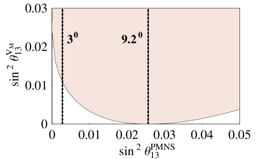
It is seen from this expression that the first two terms can cancel each other implying a vanishing $(1,3)$ entry of the $V_{M}$ matrix. In order to better investigate this issue we plot in fig.1 the quantity $\sin^{2}\theta_{13}^{V_{M}}$ as a function of $\sin^{2}\theta_{13}^{PMNS}$. All other observables are fixed at their best fit points [3, 4, 29] and we allowed the Dirac lepton phase $\phi$, the Majorana ones $\phi_{1}$ and $\phi_{2}$, and the unphysical phases of $\Omega$ to vary in the interval $[0,2\,\pi]$ with a flat distribution.

As shown in the figure, for the central value of $\theta_{13}^{PMNS}$ given in [3] the entry (1,3) of $V_{M}$ cannot be zero. However there is a small region $(\theta_{13}^{PMNS}\approx 9.2^{\circ})$ for which $\theta_{13}^{V_{M}}$ can be zero. This fact has the very important consequence of providing a sharp prediction for the unknown mixing angle $\theta_{13}^{PMNS}$. We will investigate this point in detail in the section 3.

2.2 The allowed values for $\tan^{2}\theta_{23}^{V_{M}}$, $\tan^{2}\theta_{12}^{V_{M}}$, and $\sin^{2}\theta_{13}^{V_{M}}$

Here we further investigate the possibility of $V_{M}$ to be bimaximal or tribimaximal using the fundamental equation (9). We start with a Monte Carlo simulation for the $U^{CKM}$ parameters, the $U^{PMNS}$ mixing angles, the $\Omega$ and CP phases.

We use the updated values for the $CKM$ and $PMNS$ mixing matrix, given at $95\%$CL by [29]

(22)

with

$$\rho+i\eta=\frac{\sqrt{1-A^{2}\lambda^{4}}(\overline{\rho}+i\overline{\eta})}{\sqrt{1-\lambda^{2}}\left[1-A^{2}\lambda^{4}(\overline{\rho}+i\overline{\eta})\right]}\,;$$ (23)

and  [3, 4]

(27)

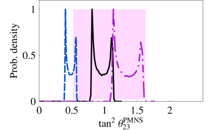
With the aid of a MonteCarlo program we generated the values for each variable: for the sine square of the lepton mixing angles and for the quark parameters $A,~{}\lambda,~{}\bar{\rho},~{}\bar{\eta}$ we took two sided Gaussian distributions with central values and standard deviations taken from eqs. (22-27). For the unknown phases we took flat random distributions in the interval $[0,2\pi]$. We divided each variable range into short bins and counted the number of occurences in each bin for all the variables, having run the program $10^{6}$ times. In this way the corresponding histogram is smooth and the number of occurences in each bin is identified with the probability density at that particular value. A comparatively high value of this probability density extending over a wide range in the variable domain means a high probability for the variable to lie in this range, therefore that such range is ’favoured’ by the data being used as MonteCarlo input. Conversely higher probability implies better compatibility with experimental data, while lower probability means poor or no compatibility with data.

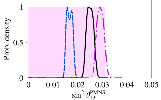
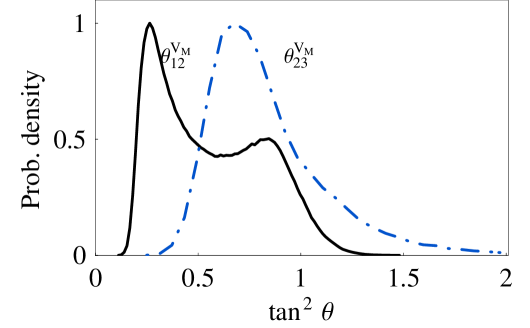
In figs 2 and 3 we report the results of this simulation. The distributions of $\tan^{2}\theta_{23}^{V_{M}}$ and $\tan^{2}\theta_{12}^{V_{M}}$ are shown in fig 2. It is seen that the range for which the value of $\tan^{2}\theta_{23}^{V_{M}}$ is compatible with experiments at $90\%$CL is the interval $[0.35,1.4]$, so that $\tan^{2}\theta_{23}^{V_{M}}=1.0$ is consistent with data. For $\tan^{2}\theta_{12}^{V_{M}}$ we obtain a range between $0.25$ and $1.1$ at $90\%$CL and so $\tan^{2}\theta_{12}^{V_{M}}=1.0$ (which corresponds to a bimaximal matrix) only within 3$\sigma$. Moreover the value $\tan^{2}\theta_{12}^{V_{M}}=0.5$ (which corresponds to a tribimaximal matrix), is well inside the allowed range. Finally in fig.3 we plot the distribution for $\sin^{2}\theta_{13}^{V_{M}}$. We see that $\sin^{2}\theta_{13}^{V_{M}}=0$ is not only allowed by the experimental data, but also it is the preferred value. In the next section we will see that this has important consequences in the model building of flavor physics.

3 Prediction for $\theta_{13}^{PMNS}$

In this section we investigate the consequences of a $V_{M}$ correlation matrix with zero (1,3) entry on the still experimentally undetermined $\theta_{13}^{PMNS}$ mixing angle. In particular we will see that the $\theta_{13}^{PMNS}$ prediction arising from eq. (9) or, equivalently,

$$U_{PMNS} = (U_{CKM}\cdot\Omega)^{-1}\cdot V_{M}$$ (28)

is quite stable against variations in the form of $V_{M}$ allowed by the data.

As previously shown (see section 2.2), the data favours a vanishing (1,3) entry in $V_{M}$. So in the whole following analysis we fix $\sin^{2}\theta_{13}^{V_{M}}=0$. We allow the $U_{CKM}$ parameters to vary, with a two-sided Gaussian distribution, within the experimental ranges given in eq. (22), while for the $\Omega$ phases in eq. (8) we take flat distributions in the interval $[0,2\pi]$.

We make Monte Carlo simulations for different values of $\theta_{12}^{V_{M}}$ and $\theta_{23}^{V_{M}}$ mixing angles, allowing $\tan^{2}\theta_{12}^{V_{M}}$ and $\tan^{2}\theta_{23}^{V_{M}}$ to vary respectively within the intervals $[0.3,1.0]$ and $[0.5,1.4]$ in consistency with the lepton and quark mixing angles (see section 2.2 and fig. 2).

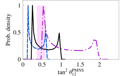
In fig.4(left) we plot the distribution of $\tan^{2}\theta_{12}^{PMNS}$ for values of the correlation matrix $V_{M}$ corresponding to $\tan^{2}\theta_{12}^{V_{M}}\in\{0.3,0.5,1.0\}$ with $\tan^{2}\theta_{23}^{V_{M}}=1.0$. From the figure we can check that for $\tan^{2}\theta_{12}^{V_{M}}=0.3,~{}{\rm and}~{}0.5$ the resulting distribution for $\tan^{2}\theta_{12}^{PMNS}$ is compatible with the experimental data. Instead maximal $\theta_{12}^{V_{M}}$ and $\theta_{23}^{V_{M}}$ taken together are disfavoured, as the solar angle is hardly compatible with the corresponding allowed interval (dot-dashed line).

In fig.4(right) we plot the distribution of $\tan^{2}\theta_{23}^{PMNS}$ for $\tan^{2}\theta_{23}^{V_{M}}\in\{0.5,1.0,1.4\}$ with $\tan^{2}\theta_{12}^{V_{M}}=0.5$. Also in these cases we see that the resulting distributions for $\tan^{2}\theta_{23}^{PMNS}$ are compatible with the experimental data.

Finally we report in fig.5 the results of our simulation for the quantity $\sin^{2}\theta_{13}^{PMNS}$. From eq. (28), the parameterization of the CKM mixing matrix in eq. (5) and the definition of the phase matrix $\Omega$ in eq. (8) we get

$$(U_{PMNS})_{13} = e^{-i\omega_{1}}\Big{[}\left(1-\frac{\lambda^{2}}{2}\right)\sin\theta_{13}^{V_{M}}e^{-i\phi^{V_{M}}}-\lambda\sin\theta_{23}^{V_{M}}\cos\theta_{13}^{V_{M}}$$ (29)

$$\quad\quad\quad+A\lambda^{3}(-\rho+i\,\eta+1)\cos\theta_{23}^{V_{M}}\cos\theta_{13}^{V_{M}}+O(\lambda^{4})\Big{]}\,,$$

so that

$$\sin^{2}\theta_{13}^{PMNS} = \sin^{2}\theta_{23}^{V_{M}}\lambda^{2}+O(\lambda^{3})\,,$$ (30)

where we have used the fact that $\sin^{2}\theta_{13}^{V_{M}}=0$ and $A\approx O(1)$.

From eq. (28) and the parameterization used for $V_{M}$ in eq. (17) we see that $\sin^{2}\theta_{13}^{PMNS}$ does not depend on $\tan^{2}\theta_{12}^{V_{M}}$. For this reason the parameter $\sin^{2}\theta_{13}^{PMNS}$ needs to be studied as a function of $\tan^{2}\theta_{23}^{V_{M}}$ only. Fixing for definiteness $\tan^{2}\theta_{12}^{V_{M}}=0.5$ and taking the three different values $\tan^{2}\theta_{23}^{V_{M}}\in\{0.5,1.0,1.4\}$, we plot in fig.6 the corresponding distributions of $\sin^{2}\theta_{13}^{PMNS}$. We note that these values of $\tan^{2}\theta_{23}^{V_{M}}$ practically cover the whole range consistent with the data (see fig.2).

From fig. 5 it is seen that the $\sin^{2}\theta_{13}^{PMNS}$ distributions are quite sharply peaked around maxima of $7.3^{\circ}$, $8.9^{\circ}$ and $9.8^{\circ}$. Recalling that the shift of this maximum is effectively determined by the parameter $\tan^{2}\theta_{23}^{V_{M}}$ which was chosen to span most of its physically allowed range, it is clear that we have a stable prediction for $\theta_{13}^{PMNS}$.

In order to better clarify this stability, we show in fig. 6 the mean and the standard deviation of $\sin^{2}\theta_{13}^{PMNS}$ obtained with our Monte Carlo simulation for the three chosen values of $\tan^{2}\theta_{23}^{V_{M}}$. In addition we plot the analytic dependence of $\sin^{2}\theta_{13}^{PMNS}$ given by eq. (30) with the central value of $\lambda$, the best fit point of $\sin^{2}\theta_{13}^{PMNS}$ and its 1$\sigma$, 2$\sigma$ and 3$\sigma$ from the analysis of ref.[3]. Our prediction for $\theta_{13}^{PMNS}$ then follows from the experimental data on $\lambda$ ,$A$, $\rho$, $\eta$, $\tan^{2}\theta_{12}^{PMNS}$ and $\tan^{2}\theta_{23}^{PMNS}$ and the values of $\tan^{2}\theta_{12}^{V_{M}}$, $\tan^{2}\theta_{23}^{V_{M}}$ are taken in the intervals $[0.3,1.0]$, $[0.5,1.4]$ respectively, as allowed by the data. For a vanishing $(1,3)$ entry of the matrix $V_{M}$ we finally find $\theta_{13}^{PMNS}$ in the interval $[7^{\circ},10^{\circ}]$.

To conclude this section we note that another prediction for a small $\theta_{13}^{PMNS}$ has recently been derived [20]

$$\theta_{13}^{PMNS}=9^{\circ}+O(sin^{3}\theta_{12}^{CKM}).$$ (31)

This follows from an assumed bimaximality of a matrix relating Dirac to Majorana neutrino states together with the assumption that neutrino mixing is described by the CKM matrix at the grand unification scale. Our approach on the other hand is free from any ad hoc assumptions. We show that it is a zero texture of the $V_{M}$ correlation matrix, namely $V_{M_{13}}=0$, together with all the experimental values of the quark and lepton mixing angles, that predicts $\theta_{13}^{PMNS}=(9\pm^{1}_{2})^{\circ}$. More importantly we show that the vanishing of this entry is favored by the data. Condition $V_{M_{13}}=0$ is compatible with $V_{M}$ being bimaximal (i.e. with two angles of $45^{\circ}$ and a vanishing one), tribimaximal (i.e. with one angle of $45^{\circ}$, one with $\tan^{2}\theta=0.5$ and a third vanishing one) or of any other form. Furthermore we make use of a phase matrix $\Omega$, see eqs. (8-9), that takes account of the mismatch between the quark and lepton phases and consider Majorana phases in the $U_{PMNS}$ matrix with a flat random distribution.

4 Summary and Conclusions

In summary, we have investigated the correlation between the CKM quark and PMNS lepton mixing matrices, arising in a large class of GUT seesaw models with specific flavor symmetries. The detailed analysis developed here uses the fact that the correlation matrix is phenomenologically compatible with a tribimaximal pattern, and marginally with a bimaximal pattern. This conclusion is different from the one obtained in previous studies [14] and is in agreement with other qualitative arguments that favor the CKM matrix to measure the deviation of the PMNS matrix from exact bimaximal mixing [21].

In our analysis we found that the mixing parameters $\tan^{2}\theta_{12}^{V_{M}}$ and $\tan^{2}\theta_{23}^{V_{M}}$ vary respectively within the intervals $[0.3,1.0]$ and $[0.5,1.4]$, while $\sin^{2}\theta_{13}^{V_{M}}$ varies in the range $[0.0,0.2]$. Moreover the preferred value for $\sin^{2}\theta_{13}^{V_{M}}$ is zero.

Using these results we investigated the phenomenological consequences of correlation matrices $V_{M}$ with zero $(1,3)$ entry. The main conclusion of this study is that this large class of models is not only compatible with the experimental data, but also that they give a robust prediction for $\theta_{13}^{PMNS}$ mixing angle

$$\theta_{13}^{PMNS}=(9{{}^{+1}_{-2}})^{\circ}\,.$$ (32)

Whereas the author of ref.[20] obtains a prediction for $\theta_{13}^{PMNS}$ in a similar range, our result cannot be regarded as a straightforward extension or generalization. In fact the condition $V_{M_{13}}=0$, which is favored by the data, is the only requirement for the prediction (32). Furthermore we modified the correlation between the CKM and PMNS mixing matrices to take account of a phase matrix $\Omega$ between the quark and lepton fields. Eq. (32) will be checked with great accuracy in the next generation of precision neutrino experiments (DCHOOZ and others).

We studied GUT models with flavor symmetry that predict a relation of the type $V_{M}=U_{CKM}\cdot\Omega\cdot U_{PMNS}$ with $V_{M_{13}}=0$. Since in supersymmetric models with $\tan\beta\leq 40$ radiative corrections are small [25, 26, 27, 28], this relation can in such cases be used at low energy as in the present paper. Hence if future dedicated experiments exclude $\theta_{13}^{PMNS}\simeq 9^{\circ}$ and supersymmetry is discovered with $\tan\beta\leq 40$, such models would be ruled out. On the other hand, a positive result from $\theta_{13}^{PMNS}$ dedicated experiments and $\tan\beta\leq 40$ would be a strong hint for these flavor symmetry models and its specific Higgs pattern.

Acknowledgments

The work of BCC was supported by Fundação para a Ciência e a Tecnologia through the grant SFRH/BPD/5719/2001. We acknowledge the MEC-INFN grant, Fundacion Seneca (Murcia) grant, CYCIT-Ministerio of Educacion (Spain) grant. M.P. and E.T-L. would like to thank Milan University for kind hospitality. M.P. would like to thank the Instituto Superior Técnico for kind hospitality.

Figure 1: The minimum value allowed for $\sin^{2}\theta_{13}^{V_{M}}$ as a function of $\sin^{2}\theta_{13}^{PMNS}$. All the other CKM and PMNS mixing parameters are fixed at their best fit points given in eq. (22-27). The unknown phases $\omega_{1}$, $\omega_{2}$, and $\omega_{3}$ of $\Omega$, the Majorana phases $\phi_{1}$, and $\phi_{2}$, and the Dirac one $\phi$ are taken to vary within the interval $[0,2\,\pi]$ with a flat distribution. We also report the values of $\theta_{13}^{PMNS}=3.0^{\circ}$ and $9.2^{\circ}$ used in the text.

Figure 2: The distributions, normalized to one at the maximum, of $\tan^{2}\theta_{12}^{V_{M}}$ (solid), and $\tan^{2}\theta_{23}^{V_{M}}$ (dot-dashed) obtained from the definition of the correlation mixing matrix $V_{M}$ given in eq. (9) by using a Monte Carlo simulation of all the experimental data.

Figure 3: The distribution, normalized to one at the maximum, of $\sin^{2}\theta_{13}^{V_{M}}$ obtained from the definition of the correlation mixing matrix $V_{M}$ given in eq. (9) by using a Monte Carlo simulation of all the experimental data. We also plot the $1\sigma$ and the $2\sigma$ lines.

Figure 4: The distribution of $\tan^{2}\theta_{12}^{PMNS}$ (left), and $\tan^{2}\theta_{23}^{PMNS}$ (right) for the CKM experimental data and for values of the correlation matrix $V_{M}$ respectively given by (left) $\tan^{2}\theta_{12}^{V_{M}}=0.3$ (dashed), $0.5$ (solid), $1.0$ (dot-dashed), $\tan^{2}\theta_{23}^{V_{M}}=1.0$, and $\sin^{2}\theta_{13}^{V_{M}}=0$; (right) $\tan^{2}\theta_{23}^{V_{M}}=0.5$ (dashed), $1.0$ (solid), $1.4$ (dot-dashed), $\tan^{2}\theta_{12}^{V_{M}}=0.5$, $\sin^{2}\theta_{13}^{V_{M}}=0$. The shaded areas represent the experimentally allowed regions at $2\sigma$ for each case.

Figure 5: The distribution of $\sin^{2}\theta_{13}^{PMNS}$ for the CKM experimental data and for values of the correlation matrix $V_{M}$ given by $\tan^{2}\theta_{12}^{V_{M}}=0.5$, $\sin^{2}\theta_{13}^{V_{M}}=0$, $\tan^{2}\theta_{23}^{V_{M}}=0.5$ (dashed), $1.0$ (solid), $1.4$ (dot-dashed). The shaded area represents the experimentally allowed region at $2\sigma$.

Figure 6: The allowed values for $\sin^{2}\theta_{13}^{PMNS}$ as a function of $\tan^{2}\theta_{23}^{V_{M}}$ under the assumption that $\sin^{2}\theta_{13}^{V_{M}}=0$. We report the central and $3\sigma$ values obtained from fig.5, and the approximate analytical dependence given in eq. (30). We also plot the experimental central value, the $1\sigma$, the $2\sigma$, and the $3\sigma$ from [3]. We fixed $\tan^{2}\theta_{12}^{V_{M}}=0.5$ for definiteness.

References

- [1] B. Pontecorvo, “Neutrino Experiments And The Question Of Leptonic-Charge Conservation,” Sov. Phys. JETP 26 (1968) 984 [Zh. Eksp. Teor. Fiz. 53 (1967) 1717].
- [2] Z. Maki, M. Nakagawa and S. Sakata, “Remarks On The Unified Model Of Elementary Particles,” Prog. Theor. Phys. 28 (1962) 870.
- [3] G. L. Fogli, E. Lisi, A. Marrone, A. Palazzo and A. M. Rotunno, “Neutrino mass and mixing parameters: A short review,” arXiv:hep-ph/0506307.
- [4] P. Aliani, V. Antonelli, M. Picariello and E. Torrente-Lujan, “The neutrino mass matrix after Kamland and SNO salt enhanced results,” arXiv:hep-ph/0309156.
- [5] M. Apollonio et al. [CHOOZ Collaboration], “Limits on neutrino oscillations from the CHOOZ experiment,” Phys. Lett. B 466 (1999) 415 [arXiv:hep-ex/9907037].
- [6] P. Aliani, V. Antonelli, M. Picariello and E. Torrente-Lujan, “Neutrino mass parameters from Kamland, SNO and other solar evidence,” Phys. Rev. D 69 (2004) 013005 [arXiv:hep-ph/0212212].
- [7] N. Cabibbo, “Unitary Symmetry And Leptonic Decays,” Phys. Rev. Lett. 10 (1963) 531.
- [8] M. Kobayashi and T. Maskawa, “CP Violation In The Renormalizable Theory Of Weak Interaction,” Prog. Theor. Phys. 49 (1973) 652.
- [9] H. Minakata and A. Y. Smirnov, “Neutrino mixing and quark lepton complementarity,” Phys. Rev. D 70, 073009 (2004) [arXiv:hep-ph/0405088].
- [10] J. Ferrandis and S. Pakvasa, “A prediction for U(e3) from patterns in the charged lepton Phys. Lett. B 603 (2004) 184 [arXiv:hep-ph/0409204].
- [11] P. H. Frampton and R. N. Mohapatra, “Possible gauge theoretic origin for quark-lepton complementarity,” JHEP 0501 (2005) 025 [arXiv:hep-ph/0407139].
- [12] S. Antusch, S. F. King and R. N. Mohapatra, “Quark lepton complementarity in unified theories,” Phys. Lett. B 618 (2005) 150 [arXiv:hep-ph/0504007].
- [13] E. Ma, “Triplicity of quarks and leptons,” Mod. Phys. Lett. A 20 (2005) 1953 [arXiv:hep-ph/0502024].
- [14] Z. z. Xing, “Nontrivial correlation between the CKM and MNS matrices,” Phys. Lett. B 618, 141 (2005) [arXiv:hep-ph/0503200].
- [15] A. Dighe, S. Goswami and P. Roy, “Quark-lepton complementarity with quasidegenerate Majorana neutrinos,” Phys. Rev. D 73 (2006) 071301 [arXiv:hep-ph/0602062].
- [16] W. Rodejohann, “A parameterization for the neutrino mixing matrix,” Phys. Rev. D 69 (2004) 033005 [arXiv:hep-ph/0309249].
- [17] P. H. Frampton, S. T. Petcov and W. Rodejohann, “On deviations from bimaximal neutrino mixing,” Nucl. Phys. B 687 (2004) 31 [arXiv:hep-ph/0401206].
- [18] A. Datta, F. S. Ling and P. Ramond, “Correlated hierarchy, Dirac masses and large mixing angles,” Nucl. Phys. B 671 (2003) 383 [arXiv:hep-ph/0306002].
- [19] A. Datta, L. Everett and P. Ramond, “Cabibbo haze in lepton mixing,” Phys. Lett. B 620 (2005) 42 [arXiv:hep-ph/0503222].
- [20] J. Harada, “Neutrino mixing and CP violation from Dirac-Majorana bimaximal mixture and quark-lepton unification,” Europhys. Lett. 75 (2006) 248 [arXiv:hep-ph/0512294].
- [21] M. Raidal, “Prediction Theta(c) + Theta(sol) = pi/4 from flavor physics: A new evidence for grand unification?,” Phys. Rev. Lett. 93 (2004) 161801 [arXiv:hep-ph/0404046].
- [22] H. Georgi and C. Jarlskog, “A New Lepton - Quark Mass Relation In A Unified Theory,” Phys. Lett. B 86 (1979) 297.
- [23] L. Wolfenstein, “Parametrization Of The Kobayashi-Maskawa Matrix,” Phys. Rev. Lett. 51 (1983) 1945.
- [24] A. J. Buras, M. E. Lautenbacher and G. Ostermaier, “Waiting for the top quark mass, K+ pi+ neutrino anti-neutrino, B(s)0 - anti-B(s)0 mixing and CP asymmetries in B decays,” Phys. Rev. D 50 (1994) 3433 [arXiv:hep-ph/9403384].
- [25] S. K. Kang, C. S. Kim and J. Lee, “Quark-lepton complementarity with renormalization effects through threshold corrections,” Phys. Lett. B 619, 129 (2005) [arXiv:hep-ph/0501029].
- [26] K. Cheung, S. K. Kang, C. S. Kim and J. Lee, “Lepton flavor violation as a probe of quark-lepton unification,” Phys. Rev. D 72 (2005) 036003 [arXiv:hep-ph/0503122].
- [27] J. R. Ellis and S. Lola, “Can neutrinos be degenerate in mass?,” Phys. Lett. B 458, 310 (1999) [arXiv:hep-ph/9904279].
- [28] S. Antusch, J. Kersten, M. Lindner, M. Ratz and M. A. Schmidt, “Running neutrino mass parameters in see-saw scenarios,” JHEP 0503 (2005) 024 [arXiv:hep-ph/0501272].
- [29] J. Charles et al. [CKMfitter Group], “CP violation and the CKM matrix: Assessing the impact of the asymmetric B factories,” Eur. Phys. J. C 41 (2005) 1 [arXiv:hep-ph/0406184 v3].