Constraining the Phase of $B_{s}-{\overline{B}}_{s}$ Mixing

Abstract

New physics contributions to $B_{s}-{\overline{B}}_{s}$ mixing can be parametrized by the size ($r_{s}^{2}$) and the phase ($2\theta_{s}$) of the total mixing amplitude relative to the Standard Model amplitude. The phase has so far been unconstrained. We first use the D$\emptyset$ measurement of the semileptonic CP asymmetry $A_{\rm SL}$ to obtain the first constraint on the semileptonic CP asymmetry in $B_{s}$ decays, $A_{\rm SL}^{s}=-0.008\pm 0.011$. Then we combine recent measurements by the CDF and D$\emptyset$ collaborations – the mass difference ($\Delta M_{s}$), the width difference ($\Delta\Gamma_{s}$) and $A_{\rm SL}^{s}$ – to constrain $2\theta_{s}$. The errors on $\Delta\Gamma_{s}$ and $A_{\rm SL}^{s}$ should still be reduced to have a sensitive probe of the phase, yet the central values are such that the regions around $2\theta_{s}\sim 3\pi/2$ and, in particular, $2\theta_{s}\sim\pi/2$, are disfavored.

Introduction. Flavor changing $b\to s$ transitions are a particularly sensitive probe of new physics. Among these, $B_{s}-{\overline{B}}_{s}$ mixing occupies a special place. New physics contributions to the mixing amplitude $M_{12}^{s}$ can be parametrized in the most general way as follows:

$$M_{12}^{s}=r_{s}^{2}\ e^{2i\theta_{s}}\ (M_{12}^{s})^{\rm SM},$$ (1)

where $(M_{12}^{s})^{\rm SM}$ is the Standard Model (SM) contribution to the mixing amplitude. Values of $r_{s}^{2}\neq 1$ and/or $2\theta_{s}\neq 0$ would signal new physics. Assuming that the new physics can affect any loop processes but is negligible for tree level processes, and that the $3\times 3$ CKM matrix is unitary (i.e. no quarks beyond the known three generations), we can use various experimental measurements to constrain the new physics parameters $r_{s}^{2}$ and $2\theta_{s}$:

1. The mass difference between the neutral $B_{s}$ states:

   $$\Delta M_{s}=(\Delta M_{s})^{\rm SM}\ r_{s}^{2}.$$ (2)

2. The width difference between the neutral $B_{s}$ states Grossman:1996er ; Dunietz:2000cr :

   $$\Delta\Gamma_{s}^{\rm CP}=\Delta\Gamma_{s}\cos 2\theta_{s}=(\Delta\Gamma_{s})^{\rm SM}\cos^{2}2\theta_{s}.$$ (3)

3. The semileptonic asymmetry in $B_{s}$ decays:

   $$A_{\rm SL}^{s}=-{\cal R}e\left(\frac{\Gamma_{12}^{s}}{M_{12}^{s}}\right)^{\rm SM}\frac{\sin 2\theta_{s}}{r_{s}^{2}}.$$ (4)

4. The CP asymmetry in $B_{s}$ decays into final CP eigenstates such as $\psi\phi$:

   $$S_{\psi\phi(CP=+)}=-\sin 2\theta_{s}.$$ (5)

Our convention here is defined by $\Delta M_{s}\equiv M_{sH}-M_{sL}$ and $\Delta\Gamma_{s}\equiv\Gamma_{sH}-\Gamma_{sL}$. The observable $\Delta\Gamma_{s}^{\rm CP}$ is defined by $\Delta\Gamma_{s}^{\rm CP}\equiv\Gamma_{-}-\Gamma_{+}$, where $\Gamma_{-}(\Gamma_{+})$ is deduced from fitting the decay rate into a final CP-odd (-even) state assuming that it is described by a single exponential. This assumption introduces an error of ${\cal O}(y_{s}^{2})=0.01$ [$y_{s}\equiv\Delta\Gamma_{s}/(2\Gamma_{s})$]. In the expressions for $\Delta\Gamma_{s}$ and $S_{\psi\phi}$ we neglect terms of ${\cal O}(\sin 2\beta_{s})=0.04$ (where $\beta_{s}=\arg[-(V_{ts}V_{tb}^{*})/(V_{cs}V_{cb}^{*})]$), while the approximation for $A_{\rm SL}^{s}$ is good to ${\cal O}[(m_{c}^{2}/m_{b}^{2})\sin 2\beta_{s}]=0.004$.

Until very recently, experiments gave only a lower bound on $\Delta M_{s}$, a large error on $\Delta\Gamma_{s}$, and no meaningful information on the CP asymmetries. Under these circumstances, there has been only a lower bound on $r_{s}^{2}$ and no constraint at all on $2\theta_{s}$.

Recently, three important experimental developments took place in this context:

• The CDF collaboration measured $\Delta M_{s}$ CDF :

  $$\Delta M_{s}=17.33^{+0.42}_{-0.21}\pm 0.07\ {\rm ps}^{-1}.$$ (6)

  (The D$\emptyset$ collaboration provided a milder two-sided bound Abazov:2006dm .)

• The D$\emptyset$ collaboration measured dzerodgs $\Delta\Gamma_{s}^{\rm CP}=-0.15\pm 0.10^{+0.03}_{-0.04}\ {\rm ps}^{-1}$. Averaging this result with the earlier measurements by CDF Acosta:2004gt and ALEPH Barate:2000kd , we obtain

  $$\Delta\Gamma_{s}^{\rm CP}=-0.22\pm 0.08\ {\rm ps}^{-1}.$$ (7)

• The D$\emptyset$ collaboration searched for the semileptonic CP asymmetry dzero ; dzpri :

  $$A_{\rm SL}=-0.0026\pm 0.0024\pm 0.0017.$$ (8)

As obvious from eq. (2), the main implication for new physics of the new result for $\Delta M_{s}$, eq. (6), is a range for $r_{s}^{2}$ which can be further translated into constraints on parameters of specific models Ligeti:2006pm ; Blanke:2006ig ; Ciuchini:2006dx ; Endo:2006dm ; Foster:2006ze ; Cheung:2006tm ; Ball:2006xx . Here, we would like to focus instead on the phase of the mixing amplitude $2\theta_{s}$. In order that a measurement of $\Delta\Gamma_{s}^{\rm CP}$ can be used to constrain $\cos^{2}2\theta_{s}$, the experimental error should be at or below the level of $(\Delta\Gamma_{s})^{\rm SM}$. The new D$\emptyset$ measurement of $\Delta\Gamma_{s}^{\rm CP}$ is the first to reach the required level. There are three necessary conditions in order that a measurement of $A_{\rm SL}$ can be used to constrain $2\theta_{s}$:

1. The experimental error on $A_{\rm SL}$ should be at or below the level of $|\Gamma_{12}^{s}/M_{12}^{s}|^{\rm SM}$;

2. An upper bound on $r_{s}^{2}$ should be available;

3. An independent upper bound on $A_{\rm SL}^{d}$ (the semileptonic asymmetry in $B_{d}$ decays) should be available.

Both the D$\emptyset$ measurement of $A_{\rm SL}$ and the CDF measurement of $\Delta M_{s}$ are thus crucial for our purposes, because they satisfy, for the first time, the first and second condition, respectively.

Relating $A_{\rm SL}$ to $A_{\rm SL}^{s}$. The semileptonic asymmetry measured at the TeVatron,

$$A_{\rm SL} \equiv \frac{\Gamma(b\bar{b}\to\mu^{+}\mu^{+}X)-\Gamma(b\bar{b}\to\mu^{-}\mu^{-}X)}{\Gamma(b\bar{b}\to\mu^{+}\mu^{+}X)+\Gamma(b\bar{b}\to\mu^{-}\mu^{-}X)}$$ (9)

$$= \frac{\Gamma_{\rm RS}^{+}\Gamma_{\rm WS}^{+}-\Gamma_{\rm RS}^{-}\Gamma_{\rm WS}^{-}}{\Gamma_{\rm RS}^{+}\Gamma_{\rm WS}^{+}+\Gamma_{\rm RS}^{-}\Gamma_{\rm WS}^{-}},$$

sums over all $B$-hadron decays. Given that the quark subprocesses are $b\to\mu^{-}X$ and $\bar{b}\to\mu^{+}X$, the right-sign (RS) and wrong-sign (WS) rates can be decomposed as follows:

$$\Gamma_{\rm RS}^{-} = f_{d}T(\overline{B}_{d}\to\overline{B}_{d}){\overline{\Gamma}}_{\rm SL}^{d}+f_{s}T(\overline{B}_{s}\to\overline{B}_{s}){\overline{\Gamma}}_{\rm SL}^{s}+f_{u}{\overline{\Gamma}}_{\rm SL}^{u},$$

$$\Gamma_{\rm RS}^{+} = f_{d}T({B}_{d}\to{B}_{d})\Gamma_{\rm SL}^{d}+f_{s}T({B}_{s}\to{B}_{s})\Gamma_{\rm SL}^{s}+f_{u}\Gamma_{\rm SL}^{u},$$

$$\Gamma_{\rm WS}^{-} = f_{d}T({B}_{d}\to\overline{B}_{d}){\overline{\Gamma}}_{\rm SL}^{d}+f_{s}T({B}_{s}\to\overline{B}_{s}){\overline{\Gamma}}_{\rm SL}^{s},$$

$$\Gamma_{\rm WS}^{+} = f_{d}T(\overline{B}_{d}\to{B}_{d})\Gamma_{\rm SL}^{d}+f_{s}T(\overline{B}_{s}\to{B}_{s})\Gamma_{\rm SL}^{s},$$ (10)

Here, $f_{q}$ is the production fraction of $B_{q}$ (we assume that there is no production asymmetry, $f_{q}={\overline{f}}_{q}$), $T$ is the time integrated probability, and $\Gamma_{\rm SL}^{q}$ (${\overline{\Gamma}}_{\rm SL}^{q}$) is the semileptonic decay rate of $B_{q}$-($\overline{B}_{q}$-)mesons. (One should think of the $q=u$ terms as representing all $b$-hadrons that do not mix, that is, the charged $B$ mesons and the $\Lambda_{b}$ baryons.)

Within our assumptions, there is no direct CP violation in semileptonic decays, that is, $\Gamma_{\rm SL}^{q}={\overline{\Gamma}}_{\rm SL}^{q}$. The time integrated probabilities fulfill $T(B_{d,s}\to B_{d,s})=T(\overline{B}_{d,s}\to\overline{B}_{d,s})$. Consequently, we have $\Gamma_{\rm RS}^{-}=\Gamma_{\rm RS}^{+}$. This leads to a considerable simplification of eq. (9):

$$A_{\rm SL}=\frac{\Gamma_{\rm WS}^{+}-\Gamma_{\rm WS}^{-}}{\Gamma_{\rm WS}^{+}+\Gamma_{\rm WS}^{-}}.$$ (11)

Thus, the semileptonic asymmetry depends only on the wrong sign rates. In particular, it is independent of the $B^{\pm}$ (and similarly of the $\Lambda_{b}$) decay rates.

To a very good approximation we expect $\Gamma_{\rm SL}^{d}=\Gamma_{\rm SL}^{s}$ (this SU(3)-flavor equality is violated only by terms of ${\cal O}(m_{s}\Lambda_{\rm QCD}/m_{b}^{2})$) which leads to

$$A_{\rm SL}=\frac{f_{d}T_{d}^{-}+f_{s}T_{s}^{-}}{f_{d}T_{d}^{+}+f_{s}T_{s}^{+}},$$ (12)

where

$$T_{q}^{\pm}=T(\overline{B}_{q}\to{B}_{q})\pm T({B}_{q}\to\overline{B}_{q}).$$ (13)

The relevant time integrated transition probabilities are as follows Branco:1999fs :

$$T(B_{q}\to\overline{B}_{q}) = \left(\frac{1-\delta_{q}}{1+\delta_{q}}\right)\frac{Z_{q}}{2\Gamma_{q}},$$

$$T(\overline{B}_{q}\to{B}_{q}) = \left(\frac{1+\delta_{q}}{1-\delta_{q}}\right)\frac{Z_{q}}{2\Gamma_{q}}$$ (14)

where ($y_{q}=\Delta\Gamma_{q}/(2\Gamma_{q})$, $x_{q}=\Delta M_{q}/\Gamma_{q}$)

$$Z_{q}\equiv\frac{1}{1-y_{q}^{2}}-\frac{1}{1+x_{q}^{2}}.$$ (15)

The quantity $\delta_{q}$ characterizes CP violation in mixing [$\delta_{q}\equiv(1-|q/p|_{q}^{2})/(1+|q/p|_{q}^{2})$]. Given that it is small, one can write to leading order $\delta_{q}=A_{\rm SL}^{q}/2$, $T^{-}_{q}=A_{\rm SL}^{q}Z_{q}/\Gamma_{q}$ and $T^{+}_{q}=Z_{q}/\Gamma_{q}$. Taking again the SU(3) limit, $\Gamma_{d}=\Gamma_{s}$ (the equality is violated at high order in $1/m_{b}$; experimentally Barberio:2006bi $\tau_{s}/\tau_{d}\sim 0.96\pm 0.04$), we obtain diffpdg

$$A_{\rm SL}=\frac{f_{d}Z_{d}A_{\rm SL}^{d}+f_{s}Z_{s}A_{\rm SL}^{s}}{f_{d}Z_{d}+f_{s}Z_{s}}.$$ (16)

Given the experimental ranges PDG $|y_{d}|=0.004\pm 0.019$ and $|y_{s}|=0.16\pm 0.06$ we can safely neglect $y_{d}^{2}$ and $y_{s}^{2}$. (Within our framework, we expect Beneke:2003az ; Ciuchini:2003ww  $y_{s}^{2}\sim 0.01$.) Using the experimental values Barberio:2006bi $f_{d}=0.4$, $f_{s}=0.1$, $x_{d}=0.78$ and $x_{s}=25.3$, we obtain

$$A_{\rm SL}\simeq 0.6A_{\rm SL}^{d}+0.4A_{\rm SL}^{s}.$$ (17)

There are two sets of measurements that, in combination, allow us to extract a range for $A_{\rm SL}^{s}$. First, we have the D$\emptyset$ measurement of $A_{\rm SL}$ (eq. (8)), which we can average together with previous measurements by the LEP experiments OPAL Abbiendi:1998av and ALEPH Barate:2000uk (we neglect here the small difference between LEP and the TeVatron regarding the measured values of $f_{d,s}$). We find

$$A_{\rm SL}=-0.0027\pm 0.0029.$$ (18)

Second, we have measurements of $A_{\rm SL}^{d}$ at the $\Upsilon(4S)$-energy by Babar Aubert:2006nf , Belle Nakano:2005jb and CLEO Jaffe:2001hz . We find

$$A_{\rm SL}^{d}=+0.0011\pm 0.0055.$$ (19)

Thus, we obtain

$$A_{\rm SL}^{s}=-0.008\pm 0.011.$$ (20)

(One could include also the Babar measurement from hadronic modes Aubert:2003hd . While this is not, strictly speaking, a measurement of $A_{\rm SL}^{d}$, it does give $1-|q/p|_{d}$. This would change the average to $A_{\rm SL}^{d}=-0.0004\pm 0.0055$ and, consequently, $A_{\rm SL}^{s}=-0.006\pm 0.011$. Our conclusions would remain unchanged.)

Constraining $2\theta_{s}$. Our constraints on $2\theta_{s}$ involve eqs. (3) and (4). As concerns $(\Gamma_{12}/M_{12})^{\rm SM}$, we use Beneke:2003az (see also Ciuchini:2003ww for a different calculation with similar results)

$${\cal R}e\left(\frac{\Gamma_{12}}{M_{12}}\right)^{\rm SM}=-0.0040\pm 0.0016.$$ (21)

As concerns $(\Delta M_{s})^{\rm SM}$, we use Blanke:2006ig

$$(\Delta M_{s})^{\rm SM} = \frac{G_{F}^{2}}{6\pi^{2}}\eta_{B}m_{B_{s}}\hat{B}_{B_{s}}F_{B_{s}}^{2}S(x_{t})|V_{tb}V_{ts}|^{2}$$ (22)

$$= 17.8\pm 4.8\ {\rm ps}^{-1}.$$

It is important to note that the range for $|V_{ts}V_{tb}|$ is derived using tree level processes and CKM unitarity. The combination of (21) and (22) gives

$$(\Delta\Gamma_{s})^{\rm SM}=-0.07\pm 0.03\ {\rm ps}^{-1}.$$ (23)

We can now fit the new physics parameters $r_{s}^{2}$ and $2\theta_{s}$ to the experimental values of eqs. (6), (7) and (20) via eqs. (2), (3) and (4). To do so, we use the SM estimates of eqs. (21), (22) and (23).

It is easy to understand the constraint on $r_{s}^{2}$ by simply using eq. (2):

$$r_{s}^{2}=\frac{(\Delta M_{s})^{\rm exp}}{(\Delta M_{s})^{\rm SM}}=0.97\pm 0.26,$$ (24)

To get a feeling for the situation concerning $2\theta_{s}$, we first use eqs. (3) and (4) separately. The $\Delta\Gamma_{s}$ measurement gives

$$\cos^{2}2\theta_{s}=\frac{(\Delta\Gamma_{s})^{\rm CP}}{(\Delta\Gamma_{s})^{\rm SM}}=3.1\pm 1.7.$$ (25)

This range disfavors (at the $1.8\sigma$ level) small $\cos^{2}2\theta_{s}$ values, that is $2\theta_{s}\sim\pi/2,3\pi/2$. The $A_{\rm SL}^{s}$ measurement gives

$$\sin 2\theta_{s}=-\frac{A_{\rm SL}^{s}}{{\cal R}e(\Gamma_{12}^{s}/M_{12}^{s})^{\rm SM}}\frac{(\Delta M_{s})^{\rm exp}}{(\Delta M_{s})^{\rm SM}}=-1.9\pm 2.8.$$ (26)

This range disfavors large positive $\sin 2\theta_{s}$ values, that is $2\theta_{s}\sim\pi/2$. The combination of the two sources of constraints should therefore disfavor the regions around $2\theta_{s}\sim\pi/2,3\pi/2$, with stronger significance for the first. This can be seen in Fig. 1, where we present the constraints in the $\cos 2\theta_{s}-\sin 2\theta_{s}$ plane. In Fig. 2 we present the constraints in the $r_{s}^{2}-2\theta_{s}$ plane. Note that eqs. (25) and (26) and Fig. 1 do not take into account the correlations between the contributions to the various observables, since they are meant to emphasize the impact of each measurement separately. The correlations are, however, fully taken into account in Fig. 2.

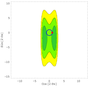
Figure 1: The constraints in the $\cos 2\theta_{s}-\sin 2\theta_{s}$ plane allowing for new physics in all loop processes. The dark green, light green and yellow regions correspond to probability higher than 0.32, 0.046, and 0.0027, respectively. The physical region ($\cos^{2}2\theta_{s}+\sin^{2}2\theta_{s}=1$) is along the blue circle. The SM point, $\cos 2\theta_{s}=+1$, $\sin 2\theta_{s}=0$, is marked with red.

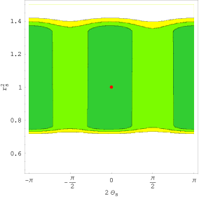
Figure 2: The constraints in the $r_{s}^{2}-2\theta_{s}$ plane allowing for new physics in all loop processes. The dark green, light green and yellow regions correspond to probability higher than 0.32, 0.046, and 0.0027, respectively. The SM point, $2\theta_{s}=0$, $r^{2}_{s}=1$, is marked with red.

We note that the ${\cal O}(30\%)$ error on $r_{s}^{2}$ is mainly theoretical: it reflects the theoretical uncertainty in $(\Delta M_{s})^{\rm SM}$. In contrast, the ${\cal O}(100\%)$ error on $\sin 2\theta_{s}$ is mainly experimental: it comes from the error in the determination of $A_{\rm SL}^{s}$. The ${\cal O}(50\%)$ error on $\cos^{2}2\theta_{s}$ has both experimental and theoretical aspects.

We learn that the constraints on $2\theta_{s}$ are still rather weak. In principle, the error on $A_{\rm SL}^{s}$ is still a factor of three larger than what is needed to have sensitivity to $\sin 2\theta_{s}$. However, since the central value for $\sin 2\theta_{s}$ happens – presumably due to statistical fluctuations – to lie below the physical region, large positive values of $\sin 2\theta_{s}$ are disfavored (at the $1\sigma$ level). The error on $\Delta\Gamma_{s}^{\rm CP}$ is closer to what is needed to be sensitive to $2\theta_{s}$ and, indeed, the resulting constraint is more significant.

We also consider a subclass of our framework, where new physics contributions are significant only in $b\to s$ transitions. This modifies the analysis in three ways:

1. We can now extract a narrower range for $(\Delta M_{s})^{\rm SM}$ by using, in addition to the direct calculation of eq. (22), an indirect calculation ckmfitter ; Bona:2005eu that makes use of experimental measurements of $b\to d$ (and $s\to d$) processes and, in particular, identify $\Delta M_{d}^{\rm exp}=\Delta M_{d}^{\rm SM}$: $(\Delta M_{s})^{\rm SM}=21.7^{+5.9}_{-4.2}\ {\rm ps}^{-1}$ statistics . The direct calculation of eq. (22) and the indirect one quoted here are essentially independent of each other. Therefore, we average over these two results and get

   $$(\Delta M_{s})^{\rm SM}=19.7\pm 3.5\ {\rm ps}^{-1}.$$ (27)

2. We can set $A_{\rm SL}^{d}=0$ and then

   $$A_{\rm SL}^{s}\simeq 2.5A_{\rm SL}=-0.007\pm 0.007.$$ (28)

3. We can now use (27) to obtain a more precise estimate of $(\Delta\Gamma_{s})^{\rm SM}$:

   $$(\Delta\Gamma_{s})^{\rm SM}=-0.08\pm 0.03\ {\rm ps}^{-1}.$$ (29)

Now we get

$$r_{s}^{2}=0.88\pm 0.16,$$ (30)

$$\cos^{2}2\theta_{s}=2.8\pm 1.6,$$ (31)

$$\sin 2\theta_{s}=-1.4\pm 1.6.$$ (32)

The situation is then quite similar to the first scenario. The smaller central value and smaller error on $r_{s}^{2}$ and on $\cos^{2}2\theta_{s}$, compared to eqs. (24) and (25), respectively, correspond to the larger central value and smaller theoretical error in eq. (27) compared to eq. (22). In contrast, the higher central value and smaller error on $\sin 2\theta_{s}$, compared to eq. (26), are both mainly a result of the shift in the central value of $r_{s}^{2}$ and, in particular, little affected by the smaller error on $(\Delta M_{s})^{\rm SM}$.

We show the contraints in the $r_{s}^{2}-2\theta_{s}$ plane in Fig. 3. As can be seen in the Figure, $2\theta_{s}=\pi/2$ is disfavored at the $2\sigma$ level.

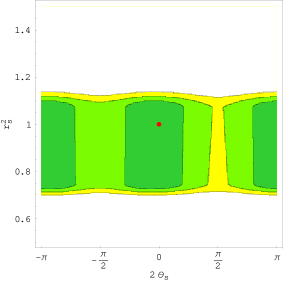
Figure 3: The constraints in the $r_{s}^{2}-2\theta_{s}$ plane allowing for new physics in $b\to s$ loop processes only. The dark green, light green and yellow regions correspond to probability higher than 0.32, 0.046, and 0.0027, respectively. The SM point, $2\theta_{s}=0$, $r^{2}_{s}=1$, is marked with red.

Conclusions. The measurement of $A_{\rm SL}$ by D$\emptyset$ probes CP violation in $B_{s}-{\overline{B}}_{s}$ mixing, $A_{\rm SL}^{s}=-0.008\pm 0.011$. In combination with the measurement of $\Delta M_{s}$ by CDF, and the measurements of $\Delta\Gamma_{s}^{\rm CP}$ by D$\emptyset$ and CDF, the CP violating phase of the mixing amplitude is constrained for the first time. The constraints are still weak. Since experiments favor large values of $\Delta\Gamma_{s}$ compared to the SM value, small values of $\cos^{2}2\theta_{s}$ (i.e. $2\theta_{s}\sim\pi/2,3\pi/2$) are disfavored. Furthermore, since experiments favor a negative $A_{\rm SL}^{s}$ (see eqs. (20) and (28)) and ${\cal R}e(\Gamma_{12}^{s}/M_{12}^{s})^{\rm SM}$ is negative, large positive values of $\sin 2\theta_{s}$ (i.e. $2\theta_{s}\sim\pi/2$) are disfavored even more strongly.

To improve the constraint, smaller experimental errors on $\Delta\Gamma_{s}$ and on $A_{\rm SL}$ are welcome. Note however that a similar improvement in the measurement of $A_{\rm SL}^{d}$ (see eq. (17)) is also required. Thus, the accuracy in determining $A_{\rm SL}^{s}$ depends on both high energy hadron machines and $\Upsilon(4S)$-energy B factories.

In principle, $A_{\rm SL}^{s}$ could also be extracted from measurements at hadron colliders only. To do this one needs, in addition to the measurement of $A_{\rm SL}$, another measurement of a CP asymmetry in semileptonic decays, with a different weight of $B_{d}$ and $B_{s}$ in the sample. (For example, requiring at least one kaon in the final state would enhance the fraction of $B_{s}$.)

Of course, the phase $2\theta_{s}$ will be strongly constrained once $S_{\psi\phi}$ is measured. Then the combination of the four measuerements – $\Delta M_{s}$, $\Delta\Gamma_{s}$, $A_{\rm SL}^{s}$ and $S_{\psi\phi}$ – will provide a test of the assumption that new physics affects only loop processes Laplace:2002ik ; Ligeti:2006pm ; Blanke:2006ig . The strength of this test will, however, be limited by theoretical uncertainties, particularly by the calculation of $\Gamma_{12}^{\rm SM}$.

Acknowledgments. We are grateful to Daria Zieminska for drawing our attention to the relevance of $\Delta\Gamma_{s}$ to our analysis and for providing us with further valuable information and advice. We are grateful to Guennadi Borissov for clarifying to us the way in which $A_{\rm SL}$ was determined by D0. We thank Andrzej Buras, Andreas Höcker, Zoltan Ligeti and Marie-Hélène Schune for useful discussions. This project was supported by the Albert Einstein Minerva Center for Theoretical Physics, and by EEC RTN contract HPRN-CT-00292-2002. The work of Y.G. is supported in part by the Israel Science Foundation under Grant No. 378/05. The research of Y.N. is supported by the Israel Science Foundation founded by the Israel Academy of Sciences and Humanities, and by a grant from the United States-Israel Binational Science Foundation (BSF), Jerusalem, Israel.

References

(1)
Y. Grossman,
Phys. Lett. B 380, 99 (1996)
[arXiv:hep-ph/9603244].
(2)
I. Dunietz, R. Fleischer and U. Nierste,
Phys. Rev. D 63, 114015 (2001)
[arXiv:hep-ph/0012219].
(3)
G. Gomez-Ceballos [CDF collaboration], talk at FPCP 2006,
http://fpcp2006.triumf.ca/talks/day3/1500/
fpcf2006.pdf.
(4)
V. Abazov [D0 Collaboration],
arXiv:hep-ex/0603029.
(5)
D0 conference note 5052.
(6)
D. Acosta et al. [CDF Collaboration],
Phys. Rev. Lett. 94, 101803 (2005)
[arXiv:hep-ex/0412057].
(7)
R. Barate et al. [ALEPH Collaboration],
Phys. Lett. B 486, 286 (2000).
(8)
B. Casey [D0 collaboration], talk at Moriond EW 2006,
http://moriond.in2p3.fr/EW/2006/Transparencies/ B.Casey.pdf.
(9)
The range that is quoted in dzero for actually
corresponds to ( is defined
below eq. (Constraining the Phase of Mixing) and is defined in eq. (15));
G. Borissov, private communication.
(10)
Z. Ligeti, M. Papucci and G. Perez,
arXiv:hep-ph/0604112.
(11)
M. Blanke, A. J. Buras, D. Guadagnoli and C. Tarantino,
arXiv:hep-ph/0604057.
(12)
M. Ciuchini and L. Silvestrini,
arXiv:hep-ph/0603114.
(13)
M. Endo and S. Mishima,
arXiv:hep-ph/0603251.
(14)
J. Foster, K. i. Okumura and L. Roszkowski,
arXiv:hep-ph/0604121.
(15)
K. Cheung, C. W. Chiang, N. G. Deshpande and J. Jiang,
arXiv:hep-ph/0604223.
(16)
P. Ball and R. Fleischer,
arXiv:hep-ph/0604249.
(17)
G. C. Branco, L. Lavoura and J. P. Silva,
“CP violation,”
(18)
E. Barberio et al. [The Heavy Flavor Averaging Group],
arXiv:hep-ex/0603003.
(19)
Our results differ from ref. Barberio:2006bi ; Abe:1996zt ; PDG ,
where our is replaced with . (Our results
do however agree with ref. Branco:1999fs .) Numerically
the difference is of and therefore
irrelevant.
(20)
F. Abe et al. [CDF Collaboration],
Phys. Rev. D 55, 2546 (1997).
(21)
S. Eidelman et al., Phys. Lett. B 592, 1 (2004) and 2005 partial
update for the 2006 edition available on the PDG WWW pages (URL:
http://pdg.lbl.gov/).
(22)
M. Beneke, G. Buchalla, A. Lenz and U. Nierste,
Phys. Lett. B 576, 173 (2003)
[arXiv:hep-ph/0307344].
(23)
M. Ciuchini et al.,
JHEP 0308, 031 (2003)
[arXiv:hep-ph/0308029].
(24)
G. Abbiendi et al. [OPAL Collaboration],
Eur. Phys. J. C 12, 609 (2000)
[arXiv:hep-ex/9901017].
(25)
R. Barate et al. [ALEPH Collaboration],
Eur. Phys. J. C 20, 431 (2001).
(26)
B. Aubert et al. [BABAR Collaboration],
Phys. Rev. Lett. 96, 251802 (2006)
[arXiv:hep-ex/0603053].
(27)
E. Nakano et al. [Belle Collaboration],
Phys. Rev. D 73, 112002 (2006)
[arXiv:hep-ex/0505017].
(28)
D. E. Jaffe et al. [CLEO Collaboration],
Phys. Rev. Lett. 86, 5000 (2001)
[arXiv:hep-ex/0101006].
(29)
B. Aubert et al. [BABAR Collaboration],
Phys. Rev. Lett. 92, 181801 (2004)
[arXiv:hep-ex/0311037].
(30)
CKMfitter Group (J. Charles et al.),
Eur. Phys. J. C41, 1-131 (2005) [hep-ph/0406184],
updated results and plots available at: http://ckmfitter.in2p3.fr
(31)
M. Bona et al. [UTfit Collaboration],
JHEP 0603, 080 (2006)
[arXiv:hep-ph/0509219].
(32)
The statistical approaches of the CKMfitter ckmfitter and UTfit
Bona:2005eu groups are different from each other. We
consistently use here the approach of ref. ckmfitter , and so
the indirect range for that we quote is the one
from ckmfitter . Had we used the methods of Bona:2005eu ,
we would expect quantitative differences but not qualitative ones.
(33)
S. Laplace, Z. Ligeti, Y. Nir and G. Perez,
Phys. Rev. D 65, 094040 (2002)
[arXiv:hep-ph/0202010].