Bicocca-FT-06-7

KA–TP–04–2006

SFB/CPP–06–20

hep-ph/0604200

Next-to-leading order QCD corrections to $Z$ boson pair production via
vector-boson fusion

Barbara Jäger¹, Carlo Oleari² and Dieter Zeppenfeld^{1 1} Institut für Theoretische Physik, Universität Karlsruhe, P.O.Box 6980, 76128 Karlsruhe, Germany

² Dipartimento di Fisica ”G. Occhialini”, Università di Milano-Bicocca, 20126 Milano, Italy

Vector-boson fusion processes are an important tool for the study of electroweak symmetry breaking at hadron colliders, since they allow to distinguish a light Higgs boson scenario from strong weak boson scattering. We here consider the channels $WW\,\mbox{$\rightarrow$}\,ZZ$ and $ZZ\,\mbox{$\rightarrow$}\,ZZ$ as part of electroweak $Z$ boson pair production in association with two tagging jets. We present the calculation of the NLO QCD corrections to the cross sections for $pp\,\mbox{$\rightarrow$}\,e^{+}e^{-}\,\mu^{+}\mu^{-}+2\;\mathrm{jets}$ and $pp\,\mbox{$\rightarrow$}\,e^{+}e^{-}\,\nu_{\mu}\bar{\nu}_{\mu}+2\;\mathrm{jets}$ via vector-boson fusion at order $\alpha_{s}\,\alpha^{6}$, which is performed in the form a NLO parton-level Monte Carlo program. The corrections to the integrated cross sections are found to be modest, while the shapes of some kinematical distributions change appreciably at NLO. Residual scale uncertainties typically are at the few percent level.

1 Introduction

One of the primary goals of the CERN Large Hadron Collider (LHC) is the discovery of the Higgs boson and a thorough investigation of the mechanism of electroweak (EW) symmetry breaking [1, 2]. In this context, vector-boson fusion (VBF) processes have emerged as a particularly interesting class of processes. Higgs boson production in VBF, i.e. the reaction $qq\,\mbox{$\rightarrow$}\,qqH$, where the Higgs decay products are detected in association with two tagging jets, offers a promising discovery channel [3] and, once its existence has been verified, will help to constrain the couplings of the Higgs boson to gauge bosons and fermions [4].

In order to distinguish possible signatures of strong weak-boson scattering from those of a light Higgs boson, a good understanding of $WW\,\mbox{$\rightarrow$}\,ZZ$ and $ZZ\,\mbox{$\rightarrow$}\,ZZ$ scattering processes, which are part of the VBF reaction $qq\,\mbox{$\rightarrow$}\,qqZZ$, is needed. This requires the computation of next-to-leading order (NLO) QCD corrections to the $qq\,\mbox{$\rightarrow$}\,qq\,ZZ$ cross section, including the leptonic decays of the $Z$ bosons. Experimentally, very clean signatures are expected from the $ZZ\,\mbox{$\rightarrow$}\,\ell^{+}\ell^{-}\ell^{\prime+}\ell^{\prime-}$ decays in VBF with four charged leptons in the final state, the disadvantage of this channel being a rather small $Z\,\mbox{$\rightarrow$}\,e^{+}e^{-}$ or $Z\,\mbox{$\rightarrow$}\,\mu^{+}\mu^{-}$ branching ratio of about 3%. The $ZZ\,\mbox{$\rightarrow$}\,\ell^{+}\ell^{-}\nu\bar{\nu}$ channel, with two undetected neutrinos, on the other hand, results in a larger number of events due to the larger $Z\,\mbox{$\rightarrow$}\,\nu\bar{\nu}$ branching ratio [5].

LO results for EW $ZZ\,jj$ production in VBF have been available for more than two decades. The first calculations [6] were performed employing the effective $W$ approximation [7], where the vector bosons radiated off the scattering quarks are treated as on-shell particles and, therefore, kinematical distributions characterizing the tagging jets cannot be predicted reliably. In the following years, exact calculations for $qq\,\mbox{$\rightarrow$}\,qq\,ZZ$ have been completed, first without $Z$ boson decay [8], and then including leptonic decays of the $Z$ bosons within the narrow width approximation [9].

We go beyond these approximations and develop a fully-flexible parton level Monte Carlo program, which allows for the calculation of cross sections and kinematical distributions for EW $ZZ\,jj$ production via VBF at NLO QCD accuracy. The program is structured in complete analogy to the respective code for EW $W^{+}W^{-}\,jj$ production presented in Ref. [10]. Here, we calculate the $t$-channel weak-boson exchange contributions to the full matrix elements for processes like $qq\,\mbox{$\rightarrow$}\,qq\,e^{+}e^{-}\,\mu^{+}\mu^{-}$ and $qq\,\mbox{$\rightarrow$}\,qq\,e^{+}e^{-}\,\nu_{\mu}\bar{\nu}_{\mu}$ at $\mathcal{O}(\alpha^{6}\alpha_{s})$. We consider all resonant and non-resonant contributions giving rise to a four charged-lepton and a two charged-lepton plus two neutrino final state, respectively. Contributions from weak-boson exchange in the $s$-channel are strongly suppressed in the phase-space regions where VBF can be observed experimentally and therefore disregarded throughout. We do not specifically require the leptons and neutrinos to stem from a genuine VBF-like production process, but also include diagrams where one or two of the $Z$ bosons are emitted from either quark line. Diagrams, where the final state leptons stem from a $\gamma\,\mbox{$\rightarrow$}\,\ell^{+}\ell^{-}$ decay or non-resonant production modes, are also taken into account. Finite-width effects are fully considered. For simplicity, we nonetheless refer to the $qq\,\mbox{$\rightarrow$}\,qq\,\ell^{+}\ell^{-}\ell^{\prime+}\ell^{\prime-}$ and $qq\,\mbox{$\rightarrow$}\,qq\,\ell^{+}\ell^{-}\nu\bar{\nu}$ processes computed this way generically as “EW $ZZ\,jj$” production.

The outline of the paper is as follows. In Sec. 2 we briefly summarize the calculation of the LO and NLO matrix elements for EW $ZZ\,jj$ production making use of the helicity techniques of Ref. [11]. Section 3 deals with phenomenological applications of the parton-level Monte Carlo program which we have developed. Conclusions are given in Sec. 4.

2 Elements of the calculation

The calculation of NLO QCD corrections to EW $ZZ\,jj$ production closely resembles our earlier work for EW $W^{+}W^{-}$ production in association with two jets [10]. The main differences lie in the electroweak aspects of the processes, while the QCD structure of the NLO corrections is very similar. The techniques developed in Ref. [10] can therefore be adapted readily and only need a brief recollection here. For simplicity, we focus on the $e^{+}e^{-}\,\mu^{+}\mu^{-}$ decay channel in the following. The application of the basic features discussed for this case to the $e^{+}e^{-}\,\nu_{\mu}\bar{\nu}_{\mu}$ leptonic final state is then straightforward.

The Feynman graphs contributing to $pp\,\mbox{$\rightarrow$}\,e^{+}e^{-}\,\mu^{+}\mu^{-}\,jj$ can be grouped in six topologies, respectively, for the 579 $t$-channel neutral-current (NC) and the 241 charged-current (CC) exchange diagrams which appear at tree level. These groups are sketched in Fig. 1

Figure 1: The six Feynman-graph topologies contributing to the Born process $uc\,\mbox{$\rightarrow$}\,uc\,e^{+}e^{-}\,\mu^{+}\mu^{-}$. Diagrams analogous to (a), (d), (e) and (f), with vector-boson emission off the lower quark line, are not shown.

for the specific NC subprocess $uc\,\mbox{$\rightarrow$}\,uc\,e^{+}e^{-}\,\mu^{+}\mu^{-}$. The first two of these correspond to the emission of two external vector bosons $V$ from the same (a) or different (b) quark lines. The remaining topologies are characterized by the vector-boson sub-amplitudes $L^{\alpha\beta}_{VV}$, $\Gamma^{\alpha}_{V}$, $T^{\alpha\beta}_{VV,\mu}$ and $T^{\alpha\beta}_{VV,e}$, which describe the tree-level amplitudes for the processes $VV\,\mbox{$\rightarrow$}\,e^{+}e^{-}\,\mu^{+}\mu^{-}$, $V\,\mbox{$\rightarrow$}\,e^{+}e^{-}\,\mu^{+}\mu^{-}$, $VV\,\mbox{$\rightarrow$}\,\mu^{+}\mu^{-}$ and $VV\,\mbox{$\rightarrow$}\,e^{+}e^{-}$. In each case, $V$ stands for a virtual $\gamma$ or $Z$ boson, and $\alpha$ and $\beta$ are the tensor indices carried by these vector bosons. The propagator factors $1/(q^{2}-m_{V}^{2}+im_{V}\Gamma_{V})$ are included in the definitions of the sub-amplitudes, which we call “leptonic tensors” in the following. Graphs for CC processes such as $us\,\mbox{$\rightarrow$}\,dc\,e^{+}e^{-}\,\mu^{+}\mu^{-}$ are obtained by replacing the $t$-channel $\gamma$ or $Z$ bosons in Fig. 1 with $W$ bosons. They give rise to the new lepton tensors $L^{\alpha\beta}_{W^{+}W^{-}}$, $T^{\alpha\beta}_{W^{+}W^{-},e}$ and $T^{\alpha\beta}_{W^{+}W^{-},\mu}$ for the sub-amplitudes $W^{+}W^{-}\,\mbox{$\rightarrow$}\,e^{+}e^{-}\,\mu^{+}\mu^{-}$, $W^{+}W^{-}\,\mbox{$\rightarrow$}\,e^{+}e^{-}$ and $W^{+}W^{-}\,\mbox{$\rightarrow$}\,\mu^{+}\mu^{-}$.

Contributions from anti-quark initiated $t$-channel processes such as $\bar{u}c\,\mbox{$\rightarrow$}\,\bar{u}c\,e^{+}e^{-}\,\mu^{+}\mu^{-}$, which emerge from crossing the above processes, are fully taken into account. On the other hand, $s$-channel exchange diagrams, where all vector bosons are time-like, contain vector-boson production with subsequent decay of one of the bosons into a pair of jets. These contributions can be safely neglected in the phase-space region where VBF can be observed experimentally, with widely-separated quark jets of large invariant mass. In the same way, $u$-channel exchange diagrams are obtained by the interchange of identical final-state (anti)quarks. Their interference with the $t$-channel diagrams is strongly suppressed for typical VBF cuts and therefore completely neglected in our calculation.

For the treatment of finite-width effects in massive vector-boson propagators we resort to a modified version of the complex-mass scheme [12], which has already been employed in Refs. [13, 10]. We globally replace vector-boson masses $m_{V}^{2}$ with $m_{V}^{2}-im_{V}\Gamma_{V}$, without changing the real value of $\sin^{2}\theta_{W}$. This procedure respects electromagnetic gauge invariance. The amplitudes for all NC and CC subprocesses are calculated and squared separately for each combination of external quark and lepton helicities. To save computer time, only the summation over the various quark helicities is done explicitely, while the four distinct lepton helicity states are considered by means of a random summation procedure.

The computation of NLO corrections is performed in complete analogy to Ref. [10]. For the real-emission contributions we encounter 2892 diagrams for the NC and 1236 for the CC processes, which are evaluated using the amplitude techniques of Ref. [11] and the leptonic tensors introduced above. Singularities in the soft and collinear regions of phase space are regularized in the dimensional-reduction scheme [14] with space-time dimension $d=4-2\epsilon$. The cancellation of these divergences with the respective poles from the virtual contributions is performed by introducing the counter terms of the dipole subtraction method [15]. Since the color and flavor structure of our processes are the same as for Higgs boson production in VBF, the analytical form of subtraction terms and finite collinear pieces is identical to the ones given in Ref. [16]. The finite parts of the virtual contributions are evaluated by Passarino-Veltman tensor reduction [17], which is implemented numerically. Here, the fast and stable computation of pentagon tensor integrals is a major issue, which is tackled by making use of Ward identities and mapping a large fraction of the pentagon diagrams onto box-type contributions with the methods developed in [10]. The residual pentagon contributions amount only to about 1 $\permil$ of the cross sections presented below.

The results obtained for the Born amplitude, the real emission and the virtual corrections have been tested extensively. For the tree-level amplitude, we have performed a comparison to the fully automatically generated results provided by MadGraph [18], and we found agreement at the $10^{-13}$ level. In the same way, the real emission contributions have been checked. For the latter, also QCD gauge invariance has been tested, which turned out to be fulfilled within the numerical accuracy of the program. The numerical stability of the finite parts of the pentagon contributions is monitored by checking numerically that they satisfy electroweak Ward identities with a relative error less than $\delta=1.0$. This criterion is violated by about 3% of the generated events. The contributions from these phase-space points to the finite parts of the pentagon diagrams are disregarded and the remaining pentagon parts are corrected by a global factor for this loss. In Ref. [10] we found that this procedure gives a stable result for the pentagon contributions when varying the accuracy parameter $\delta$.

3 Numerical results

The cross-section contributions discussed in the previous section are implemented in a fully-flexible parton-level Monte Carlo program for EW $ZZjj$ production at NLO QCD accuracy, very similar to the programs for $Hjj$, $Vjj$ and $W^{+}W^{-}jj$ production in VBF described in Refs. [16], [13] and [10].

Throughout our calculation, fermion masses are set to zero and external $b$- and $t$-quark contributions are neglected. However, the code does allow the inclusion of $b$-quark initiated sub-processes for NC exchange where internal top-quark propagators do not occur. For the Cabibbo-Kobayashi-Maskawa matrix, $V_{CKM}$, a diagonal form equal to the identity matrix has been used, which yields the same results as a calculation employing the exact $V_{CKM}$ when the summation over all quark flavors is performed.

We use the CTEQ6M parton distributions with $\alpha_{s}(m_{Z})=0.118$ at NLO, and the CTEQ6L1 set at LO [19]. We chose $m_{Z}=91.188$ GeV, $m_{W}=80.419$ GeV and $G_{F}=1.166\times 10^{-5}/$GeV² as electroweak input parameters. Thereof, $\alpha_{QED}=1/132.54$ and $\sin^{2}\theta_{W}=0.22217$ are computed via LO electroweak relations. To reconstruct jets from final-state partons, the $k_{T}$ algorithm [20, 21] is used with resolution parameter $D=0.8$.

Partonic cross sections are calculated for events with at least two hard jets, which are required to have

$$p_{Tj}\geq 20~{}{\rm GeV}\,,\qquad\qquad|y_{j}|\leq 4.5\,.$$ (3.1)

Here $y_{j}$ denotes the rapidity of the (massive) jet momentum which is reconstructed as the four-vector sum of massless partons of pseudorapidity $|\eta|<5$. The two reconstructed jets of highest transverse momentum are called “tagging jets”. At LO, they are the final-state quarks which are characteristic of vector-boson fusion processes. Backgrounds to VBF are significantly reduced by requiring a large rapidity separation of the two tagging jets. We therefore impose the cut

$$\Delta y_{jj}=|y_{j_{1}}-y_{j_{2}}|>4\;.$$ (3.2)

Furthermore, the tagging jets are imposed to reside in opposite detector hemispheres,

$$y_{j_{1}}\cdot y_{j_{2}}<0\,,$$ (3.3)

with an invariant mass

$$M_{jj}>600~{}{\rm GeV}\;.$$ (3.4)

These cuts render the LO differential cross section for $ZZjj$ finite, since they enforce finite scattering angles for the two quark jets. For the NLO contributions, initial-state singularities, due to collinear $q\,\mbox{$\rightarrow$}\,gq$ and $g\,\mbox{$\rightarrow$}\,q\bar{q}$ splitting, are factorized into the respective quark and gluon distribution functions of the proton. Additional divergences, stemming from the $t$-channel exchange of low-virtuality photons in real-emission diagrams, are avoided by imposing a cut on the virtuality of the photon, $Q^{2}_{\gamma,\mathrm{min}}=4$ GeV². Events that do not pass this cut give rise to a collinear $q\,\mbox{$\rightarrow$}\,q\gamma$ singularity, which is considered to be part of the QCD corrections to $p\gamma\,\mbox{$\rightarrow$}\,ZZjj$ and not calculated here.

In the discussion of the $pp\,\mbox{$\rightarrow$}\,\ell^{+}\ell^{-}\ell^{\prime+}\ell^{\prime-}\,jj$ channel, we focus on the leptonic final state $e^{+}e^{-}\,\mu^{+}\mu^{-}$ throughout. Results for the four lepton final state with any combination of electrons and/or muons (i.e. $e^{+}e^{-}\mu^{+}\mu^{-}$, $e^{+}e^{-}e^{+}e^{-}$ and $\mu^{+}\mu^{-}\mu^{+}\mu^{-}$) are obtained by multiplying the respective numbers for $e^{+}e^{-}\mu^{+}\mu^{-}$ by a factor of two. This procedure neglects very small Pauli-interference effects for identical charged leptons, however. Similarly, the $e^{+}e^{-}\,\nu_{\mu}\bar{\nu}_{\mu}$ combination on which we concentrate, is related to an arbitrary two lepton plus two neutrino final state in the case of $pp\,\mbox{$\rightarrow$}\,\ell^{+}\ell^{-}\nu\bar{\nu}\,jj$ production: Here, a factor of six is needed to take into account all neutrino species and two families of charged leptons. To ensure that the charged leptons are well observable, we impose the lepton cuts

$$p_{T\ell}\geq 20~{}{\rm GeV}\,,\qquad|\eta_{\ell}|\leq 2.5\,,\qquad\triangle R_{j\ell}\geq 0.4\,,$$

$$m_{\ell\ell}\geq 15~{}{\rm GeV}\,,\qquad\triangle R_{\ell\ell}\geq 0.2\,,$$ (3.5)

where $\triangle R_{j\ell}$ and $\triangle R_{\ell\ell}$ denote the jet-lepton and lepton-lepton separation in the rapidity-azimuthal angle plane. In addition, the charged leptons are required to fall between the rapidities of the two tagging jets

$$y_{j,min}<\eta_{\ell}<y_{j,max}\,.$$ (3.6)

In order to compute the full cross section for EW $ZZjj$ production, contributions from the Higgs boson resonance, $qq\,\mbox{$\rightarrow$}\,Hqq\,\mbox{$\rightarrow$}\,ZZqq$, as well as from the $ZZ$ continuum have to be considered. A representative for the latter, which effectively starts at the $Z$-pair threshold, is obtained (for a Higgs mass below the $Z$-pair threshold) by imposing a cut on the four-lepton invariant mass of

$$M_{ZZ}=\sqrt{(p_{\ell^{+}}+p_{\ell^{-}}+p_{\ell^{\prime+}}+p_{\ell^{\prime-}})^{2}}>m_{H}+10\;{\rm GeV}\;,$$ (3.7)

and correspondingly for the $\ell^{+}\ell^{-}\nu\bar{\nu}$ final state. Since the contribution from the Higgs boson resonance has already been computed in Ref. [16], we focus on the $ZZ$ continuum in the following, if not stated otherwise, and assume $m_{H}=120$ GeV.

The continuum cross section $\sigma_{\rm cuts}$ for EW $e^{+}e^{-}\,\nu_{\mu}\bar{\nu}_{\mu}\,jj$ production, within the cuts of Eqs. (3.1)–(3.7), is shown in Fig. 2.

Figure 2: Scale dependence of the total EW $e^{+}e^{-}\,\nu_{\mu}\bar{\nu}_{\mu}\,jj$ cross section at LO and NLO within the cuts of Eqs. (3.1)–(3.7) for $pp$ collisions at the LHC. The NLO curves show $\sigma_{\rm cuts}^{\rm NLO}$ as functions of the scale parameter $\xi$ for three different cases: $\mu_{F}=\mu_{R}=\xi m_{Z}$ (solid red), $\mu_{F}=\xi m_{Z}$ and $\mu_{R}=m_{Z}$ (dot-dashed blue), $\mu_{F}=m_{Z}$ and $\mu_{R}=\xi m_{Z}$ (dashed green). The LO cross section depends only on $\mu_{F}$ (dotted black line).

The figure illustrates the dependence of the NLO cross section on the renormalization and factorization scales, $\mu_{R}$ and $\mu_{F}$, which are taken as multiples of the $Z$ mass,

$$\mu_{R}=\xi_{R}\,m_{Z}\;,\qquad\qquad\mu_{F}=\xi_{F}\,m_{Z}\;.$$ (3.8)

The LO cross section only depends on $\mu_{F}=\xi_{F}\,m_{Z}$. By varying the scale factor $\xi_{F}=\xi$ in the range $0.1\div 10$, the value of $\sigma_{\rm cuts}^{\rm LO}$ changes by almost a factor of two, indicating the theoretical uncertainty of the LO calculation. The strong scale dependence is reduced substantially after the inclusion of NLO corrections. For $\sigma_{\rm cuts}^{\rm NLO}$ we study three different cases: $\xi_{F}=\xi_{R}=\xi$ (solid red line), $\xi_{F}=\xi$, $\xi_{R}=1$ (dot-dashed blue line), and $\xi_{F}=1$, $\xi_{R}=\xi$ (dashed green line). The latter curve illustrates clearly the weak dependence of $\sigma_{\rm cuts}^{\rm NLO}$ on the renormalization scale, which can be understood from the fact that $\alpha_{s}(\mu_{R})$ enters only at NLO, while the LO cross section is completely independent of $\mu_{R}$. Also the factorization-scale dependence of the full cross section is rather low, such that the variation of $\sigma_{\rm cuts}^{\rm NLO}$ with the scale parameter amounts to less than 2% for all cases in the interesting range $0.5<\xi<2$. In the following, we fix the scales to $\mu_{F}=\mu_{R}=m_{Z}$.

As a representative for the observables characterizing the tagging jets, we show the invariant mass distribution of the tagging-jet pair, $d\sigma/dM_{jj}^{\rm tag}$, for EW $e^{+}e^{-}\,\mu^{+}\mu^{-}\,jj$ production in Fig. 3.

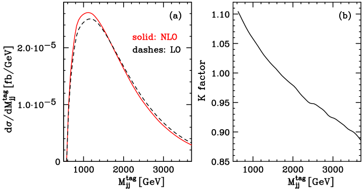
Figure 3: Invariant-mass distribution of the tagging jets in EW $e^{+}e^{-}\,\mu^{+}\mu^{-}\,jj$ production at the LHC. Panel (a) shows the NLO (solid red) and the LO results (dashed black). Panel (b) displays the K factor as defined in Eq. (3.9).

The shape of the distribution at NLO differs from the respective LO result. This is emphasized in panel (b) of the figure, where we show the dynamical K factor, defined as

$$K(x)=\frac{d\sigma_{\rm NLO}/dx}{d\sigma_{\rm LO}/dx}\;.$$ (3.9)

Due to the extra parton emerging in the real-emission contributions to the NLO cross section, the quarks which constitute the tagging jets tend to have smaller transverse momenta than at LO, thereby giving rise to lower values of their invariant mass. The transverse-momentum distributions of the tagging jets, per se, exhibit K factors in the range $0.8\div 1.4$. On the other hand, angular distributions, such as the azimuthal angle between the tagging jets, display rather uniform K factors for the scale choice $\mu_{F}=\mu_{R}=m_{Z}$. For this particular scale choice, the total cross section is barely affected by the inclusion of NLO corrections, leading to a K factor of 0.99.

Finally, we show the distribution of the invariant mass of the $e^{+}e^{-}\,\mu^{+}\mu^{-}$ system, which is given by Eq. (3.7) and can be fully reconstructed experimentally. It is very sensitive to a light Higgs boson, showing a pronounced resonance behavior for $m_{H}\lesssim 800$ GeV. For values of $m_{H}$ of the order of 1 TeV, the peak is diluted due to the large corresponding width of the Higgs boson ($\Gamma_{H}\approx 500$ GeV) and the signal is distributed over a wide range in $M_{ZZ}$. Figure 4

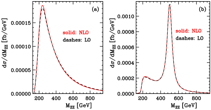
Figure 4: Panel (a): distribution of the four lepton invariant mass in EW $e^{+}e^{-}\,\mu^{+}\mu^{-}\,jj$ continuum production at the LHC, within the cuts of Eqs. (3.1)–(3.7) with $m_{H}=120$ GeV. Panel (b) shows the same observable when the contribution from a Higgs boson of mass $m_{H}=500$ GeV is included. In each case, NLO (red solid) and LO (black dashed) results are shown.

illustrates the resonance behavior of $M_{ZZ}$: panel (a) shows the $M_{ZZ}$ distribution for the continuum production of four charged leptons. Panel (b) displays the same observable, but now including the resonance contribution from a Higgs boson with $m_{H}=500$ GeV.

One remarkable feature of Fig. 4 is that LO and NLO results are virtually indistinguishable, for the scale choice $\mu_{F}=\mu_{R}=m_{Z}$. For the $M_{ZZ}$ distribution, the invariant mass of the $Z$ pair is another possible scale choice, which, however, would lead to substantially reduced LO differential cross section predictions at high values of $M_{ZZ}$. One finds, for example, a decrease by a factor of $\approx 1.8$ in $d\sigma^{\rm LO}/dM_{ZZ}$ at $M_{ZZ}=1.5\;{\rm TeV}$ when changing $\mu_{F}=m_{Z}$ to $\mu_{F}=M_{ZZ}$, which largely is due to an underestimate of the LO parton distributions at large Feynman-$x$. The NLO prediction, on the other hand, decreases by about 13% compared to our default choice $\mu_{F}=\mu_{R}=m_{Z}$, demonstrating the precision gained by including the NLO corrections.

4 Conclusions

In this paper we have presented first results for EW $ZZ\,jj$ production at NLO QCD accuracy, obtained with a fully-flexible parton-level Monte Carlo program that allows for a straightforward implementation of realistic experimental cuts. The integrated cross sections for the two processes $pp\,\mbox{$\rightarrow$}\,e^{+}e^{-}\,\mu^{+}\mu^{-}\,jj$ and $pp\,\mbox{$\rightarrow$}\,e^{+}e^{-}\,\nu_{\mu}\bar{\nu}_{\mu}\,jj$ were found to exhibit K factors around 0.99, which shows that higher-order corrections are under excellent control. Larger NLO contributions are obtained for some kinematical distributions with dynamical K factors in the range $0.8\div 1.4$. These results hold for a default scale choice of $\mu=m_{Z}$. Leading order results can change substantially, by up to a factor of 2, for other scale choices, while NLO results are very stable, demonstrating the value of the NLO corrections. An estimate of the theoretical uncertainty of the NLO calculation is provided by the scale variation of cross sections, within VBF cuts. It amounts to about 2% for integrated cross sections and, in extreme cases, up to 10% for distributions, when changing scales by a factor of two. Similar uncertainties are induced by the present errors on parton distribution functions, which, in the analogous case of Higgs boson production in VBF, were found to be about $\pm 3.5$% [16].

References

- [1] ATLAS Collaboration, ATLAS TDR, Report No. CERN/LHCC/99-15 (1999); E. Richter-Was and M. Sapinski, Acta Phys. Pol. B 30, 1001 (1999); B. P. Kersevan and E. Richter-Was, Eur. Phys. J. C 25, 379 (2002) [arXiv:hep-ph/0203148].
- [2] G. L. Bayatian et al., CMS Technical Proposal, Report No. CERN/LHCC/94-38x (1994); R. Kinnunen and D. Denegri, CMS Note No. 1997/057; R. Kinnunen and A. Nikitenko, Report No. CMS TN/97-106; R. Kinnunen and D. Denegri, arXiv:hep-ph/9907291; V. Drollinger, T. Müller and D. Denegri, arXiv:hep-ph/0111312.
- [3] D. L. Rainwater, PhD thesis, arXiv:hep-ph/9908378.
- [4] D. Zeppenfeld, R. Kinnunen, A. Nikitenko and E. Richter-Was, Phys. Rev. D 62, 013009 (2000) [arXiv:hep-ph/0002036]; D. Zeppenfeld, in Proc. of the APS/DPF/DPB Summer Study on the Future of Particle Physics, Snowmass, 2001 edited by N. Graf, eConf C010630, p. 123 (2001) [arXiv:hep-ph/0203123]; A. Belyaev and L. Reina, JHEP 0208, 041 (2002) [arXiv:hep-ph/0205270]; M. Dührssen et al., Phys. Rev. D 70, 113009 (2004) [arXiv:hep-ph/0406323].
- [5] R. N. Cahn and M. S. Chanowitz, Phys. Rev. Lett. 56, 1327 (1986).
- [6] M. J. Duncan, Phys. Lett. B 179, 393 (1986); A. Abbasabadi and W. W. Repko, Nucl. Phys. B292, 461 (1987).
- [7] R. N. Cahn and S. Dawson, Phys. Lett. B 136, 196 (1984) [Erratum-ibid. B 138, 464 (1984)]; S. Dawson, Nucl. Phys. B249, 42 (1985); M. J. Duncan, G. L. Kane and W. W. Repko, Nucl. Phys. B272, 517 (1986).
- [8] D. A. Dicus, S. W. Wilson and R. Vega, Phys. Lett. B 192, 21 (1987).
- [9] U. Baur and E. W. N. Glover, Nucl. Phys. B347, 12 (1990); U. Baur and E. W. N. Glover, Phys. Rev. D 44 99 (1991).
- [10] B. Jäger, C. Oleari and D. Zeppenfeld, arXiv:hep-ph/0603177.
- [11] K. Hagiwara and D. Zeppenfeld, Nucl. Phys. B274, 1 (1986); K. Hagiwara and D. Zeppenfeld, Nucl. Phys. B313, 560 (1989).
- [12] A. Denner, S. Dittmaier, M. Roth and D. Wackeroth, Nucl. Phys. B560, 33 (1999) [arXiv:hep-ph/9904472].
- [13] C. Oleari and D. Zeppenfeld, Phys. Rev. D 69, 093004 (2004) [arXiv:hep-ph/0310156].
- [14] Warren Siegel, Phys. Lett. B 84, 193 (1979); Warren Siegel, Phys. Lett. B 94, 37 (1980).
- [15] S. Catani and M. H. Seymour, Nucl. Phys. B485, 291 (1997) [Erratum-ibid. B510, 503 (1997)] [arXiv:hep-ph/9605323].
- [16] T. Figy, C. Oleari and D. Zeppenfeld, Phys. Rev. D 68, 073005 (2003) [arXiv:hep-ph/0306109].
- [17] G. Passarino and M. J. Veltman, Nucl. Phys. B160, 151 (1979).
- [18] T. Stelzer and W. F. Long, Comput. Phys. Commun. 81, 357 (1994) [arXiv:hep-ph/9401258]; F. Maltoni and T. Stelzer, JHEP 0302, 027 (2003) [arXiv:hep-ph/0208156].
- [19] J. Pumplin, D. R. Stump, J. Huston, H. L. Lai, P. Nadolsky and W. K. Tung, JHEP 0207, 012 (2002) [arXiv:hep-ph/0201195].
- [20] S. Catani, Yu. L. Dokshitzer and B. R. Webber, Phys. Lett. B 285 291 (1992); S. Catani, Yu. L. Dokshitzer, M. H. Seymour and B. R. Webber, Nucl. Phys. B406 187 (1993); S. D. Ellis and D. E. Soper, Phys. Rev. D 48 3160 (1993).
- [21] G. C. Blazey et al., arXiv:hep-ex/0005012.