Bootstrapping One-Loop QCD Amplitudes
with General Helicities

Abstract

The recently developed on-shell bootstrap for computing one-loop amplitudes in non-supersymmetric theories such as QCD combines the unitarity method with loop-level on-shell recursion. For generic helicity configurations, the recursion relations may involve undetermined contributions from non-standard complex singularities or from large values of the shift parameter. Here we develop a strategy for sidestepping difficulties through the use of pairs of recursion relations. To illustrate the strategy, we present sets of recursion relations needed for obtaining $n$-gluon amplitudes in QCD. We give a recursive solution for the one-loop $n$-gluon QCD amplitudes with three or four color-adjacent gluons of negative helicity and the remaining ones of positive helicity. We provide an explicit analytic formula for the QCD amplitude $A_{6;1}(1^{-},2^{-},3^{-},4^{+},5^{+},6^{+})$, as well as numerical results for $A_{7;1}(1^{-},2^{-},3^{-},4^{+},5^{+},6^{+},7^{+})$, $A_{8;1}(1^{-},2^{-},3^{-},4^{+},5^{+},6^{+},7^{+},8^{+})$, and $A_{8;1}(1^{-},2^{-},3^{-},4^{-},5^{+},6^{+},7^{+},8^{+})$. We expect the on-shell bootstrap approach to have widespread applications to phenomenological studies at colliders.

I Introduction

The success of the forthcoming experimental program at CERN’s Large Hadron Collider will depend in part on theoretical tools. Our ability to find and understand new physics at the TeV scale will rely on the quality of predictions for a variety of known-physics processes. A classic example is the $W+4{\rm\ jet}$ background to top-quark production. Tools to perform higher-order corrections to a wide variety of processes in the component gauge theories of the Standard Model will play an important role. Tree-level scattering amplitudes provide the basic predictions for cross sections for Standard Model processes. However, next-to-leading order (NLO) QCD corrections are typically quite large. One-loop QCD amplitudes, which enter at NLO, are therefore needed in order to reduce theoretical uncertainties to the level of 10% or so. An important set of Standard Model backgrounds to new physics dictates the computation of new one-loop amplitudes for processes containing one or more vector bosons ($W$s, $Z$s, and photons) and multiple jets.

Experience has shown that while methods relying on direct analytical evaluation of Feynman diagrams can be used for five-point processes, they have not proven powerful enough to compute six-point processes or beyond in QCD. The recent development of semi-numerical approaches GieleGloverNumerical ; EGZ ; EGZ06 shows promise for improving traditional capabilities. All helicity configurations for the six-gluon amplitude have been evaluated numerically in this way, and numerical results presented for a single phase-space point EGZ06 . These results are also of utility in confirming analytic expressions. (For other numerical or semi-numerical approaches, see ref. OtherNumerical .)

On-shell methods for computing amplitudes can be much more efficient than Feynman diagrams, because they avoid gauge non-invariant intermediate states and instead focus on the key analytic properties that any physical amplitude must satisfy. The unitarity-based method Neq4Oneloop ; Neq1Oneloop ; BernMorgan ; UnitarityMachinery was applied long ago, not only to six-point processes, but also to all-multiplicity amplitudes, for particular configurations of external helicities. Early applications of the method were generally restricted, for practical reasons, to supersymmetric theories or to the polylogarithmic part of QCD amplitudes. This practical restriction arose from the greater complexity of $D$-dimensional unitarity calculations, required for full QCD amplitudes in this approach.

A key feature of the unitarity method is that new amplitudes are constructed with only on-shell tree-level amplitudes (which are generally quite simple) as inputs. A number of related techniques have emerged in the past two years, including the application of maximally-helicity-violating (MHV) vertices CSW ; Risager to loop calculations BST ; BBSTQCD and the use CachazoAnomaly ; BCF7 of the holomorphic anomaly HolomorphicAnomaly to evaluate the cuts.

More recent improvements to the unitarity method BCFUnitarity ; BMSTUnitarity ; BBCFSQCD ; BFM use complex momenta within generalized unitarity ZFourPartons ; TwoLoopSplit ; NeqFourSevenPoint , allowing, for example, a simple and purely algebraic determination of all box integral coefficients. (The name ‘generalized unitarity’, as applied to amplitudes for massive particles, can be traced back to ref. Eden .) In ref. BBCFSQCD , Britto, Buchbinder, Cachazo and Feng developed efficient techniques for evaluating generic one-loop unitarity cuts, by using spinor variables and performing the cut integration via residue extraction. Quite recently, Britto, Feng and Mastrolia BFM further extended these techniques and completed the computation of all cut-containing terms for the six-gluon helicity amplitudes. The cut-containing terms for other helicity configurations, and for other components of the amplitudes, were obtained in refs. Neq4Oneloop ; Neq1Oneloop ; NeqOneNMHVSixPt ; DunbarBoxN1 ; RecurCoeff ; BBCFSQCD . The only terms now missing in the analytic expressions for the six-gluon amplitudes are the pure-rational ones. The computation of the rational terms, in these and more general amplitudes, is the subject of this paper.

In a previous paper Bootstrap , three of the authors presented a systematic, recursive bootstrap approach to making high-multiplicity QCD calculations practical within the framework of the unitarity-based method. It complements the use of four-dimensional unitarity for logarithmic and polylogarithmic terms with an on-shell recursion relation BCFRecurrence ; BCFW ; OnShellRecurrenceI ; Qpap for the purely-rational terms. This approach systematizes a unitarity-factorization bootstrap previously applied to the amplitudes for $e^{+}e^{-}\to~{}4$ partons ZFourPartons . It has already been used to solve for infinite sequences of one-loop $n$-gluon helicity amplitudes, in particular the MHV amplitudes containing two color-adjacent negative-helicity gluons and $(n-2)$ positive-helicity ones FordeKosower . These papers do not explain how to attack more general helicity configurations. That is the purpose of the present paper: to extend the range of applicability of the recursive bootstrap method to cover as generic a helicity configuration as possible.

Recursion relations have long been used in QCD BGRecurrence ; DAKRecurrence , and are an elegant and efficient means for computing tree-level amplitudes. Other related approaches Alpgen , as well as computer-driven approaches such as MadGraph Madgraph , have also been employed. Stimulated by the compact forms of seven- and higher-point tree amplitudes NeqFourSevenPoint ; NeqFourNMHV ; RSVNewTree that emerged from studying infrared consistency equations UniversalIR for one-loop amplitudes (computed using the unitarity-based method), Britto, Cachazo and Feng wrote down BCFRecurrence a new set of tree-level recursion relations. The new recursion relations differ in that they employ only on-shell amplitudes (at complex values of the external momenta). A simple and very general proof of the relations, using special continuations (shifts) of the external momenta in terms of a complex variable $z$, was then given by Britto, Cachazo, Feng and Witten BCFW . The power of this type of recursion relation follows from the generality of the proof, which relies only on factorization and Cauchy’s theorem. (The numerical efficiency of these recursion relations, with respect to the older, off-shell recursion relations BGRecurrence ; DAKRecurrence and those based on MHV vertices CSW ; BBKR , has been studied recently DTW .) On-shell recursive methods have also yielded compact expressions for tree amplitudes in gravity Gravity as well as gauge theory TreeRecurResults , and have been extended to theories with massive scalars and fermions GloverMassive ; Massive . They even provide a derivation Risager of the Cachazo–Svrček–Witten representation of amplitudes in terms of MHV vertices CSW . Many of these developments, as well as the resurgence of interest in unitarity methods, were inspired by the development of twistor string theory WittenTopologicalString .

The unitarity-based method Neq4Oneloop ; Neq1Oneloop turns a general property of field theories — the unitarity of the (perturbative) $S$-matrix — into a practical technique for computing cut-containing terms in amplitudes. In a similar spirit, on-shell recursion relations turn another general property — factorization on poles in intermediate states — into a technique for computing rational terms in amplitudes. The idea of using factorization as a computational tool goes back to the computation of the $Z\rightarrow 4$ parton one-loop matrix elements ZFourPartons (or equivalently, by crossing, the virtual diagrams for $pp\rightarrow W,Z+{\rm jets}$), wherein all terms consistent with the helicity assignments were written down, and collinear limits used to isolate the correct ones and their coefficients. This approach gets harder to apply as the number of external legs increases, because of the difficulty of finding terms with the correct factorization properties. The one-loop on-shell recursion relations Bootstrap provide a practical and systematic method for constructing the rational terms, avoiding this difficulty. Moreover, in special cases, when certain criteria on the unitarity cuts are satisfied RecurCoeff , it is also possible to obtain the rational coefficients of the cut-containing (poly)logarithmic terms via on-shell recursion relations.

The factorization properties of one-loop amplitudes in gauge theories, as a function of real Minkowski four-momenta, have been known for a long time. We may distinguish two different cases. In the first case, dubbed “multi-particle” factorization, the momentum going on shell is a sum of three or more external momenta. In the second case, called “collinear” factorization, it is a sum of two momenta. The standard derivations describe how amplitudes factorize in either of these limits, when all momenta involved are real. The implementation of on-shell recursion relations requires a generalization of these factorizations to complex momenta. This generalization is straightforward, both at tree level and at one loop, for multi-particle factorization. The generalization is also straightforward at tree level for collinear factorization. This is no longer true at one loop.

The heuristic reason why collinear factorization is more intricate with complex momenta is that one cannot define a nonsingular all-massless three-point kinematics with real momenta, while one can using complex momenta. At the loop level, the complexity of complex collinear factorization is reflected in the appearance of double poles and ‘unreal’ poles in scattering amplitudes OnShellRecurrenceI ; Qpap . As yet, we have no general theorems providing universal factorization formulæ in these “non-standard” cases. In previous computations Bootstrap ; FordeKosower of one-loop amplitudes with two color-adjacent negative legs, these problems could be sidestepped by making special choices in constructing recursion relations. Within the framework of ref. Bootstrap , we must choose momentum shifts under which the amplitude vanishes at large shift parameter $z$. Otherwise, the contour integral over $z$ which gives rise to the recursion relation would receive an undetermined contribution from large $z$. In the case of MHV $n$-gluon amplitudes, which contain only two negative-helicity gluons, it is possible to make such a choice and yet avoid channels with unknown factorizations Bootstrap ; FordeKosower ; MHVQCDLoop .

For general helicity configurations, however, it is no longer possible to do this. It might seem that we should therefore study the ‘difficult’ channels, and attempt to derive a universal form for their complex-momentum factorization. It turns out, however, that it is easier to relax the other requirement, that of a vanishing amplitude at large shift parameter $z$. Indeed, in ref. OnShellRecurrenceI it was shown that, if we somehow knew the large-$z$ behavior of an amplitude in a recursion, then a non-vanishing behavior posed no problems; the recursion relations still reconstructed the remaining terms in an amplitude correctly. Our aim here is to show how to determine the large-$z$ behavior of amplitudes from scratch. We will do so by using an auxiliary recursion relation, constructed by considering pairs of momentum shifts, one in the parameter $z$ and a second involving different external legs and another parameter $w$. With these additional terms in hand, we can follow the approach of ref. Bootstrap for the remainder of the calculation, computing recursive and overlap diagrams to add to the cut-containing terms.

As an illustration of our method, we will compute one-loop corrections to a class of next-to-maximally-helicity-violating (NMHV) $n$-gluon amplitudes in QCD, those with three adjacent negative helicities in the color ordering, $A_{n;1}^{1\mbox{-}\rm loop}({-}{-}{-}{+}{+}\cdots{+}{+})$. Under a supersymmetric decomposition GGGGG , these amplitudes may be thought of as composed of ${\cal N}=4$ and ${\cal N}=1$ supersymmetric pieces together with a non-supersymmetric (${\cal N}=0$) scalar loop contribution. The ${\cal N}=4$ contributions were computed in ref. NeqFourNMHV , and the ${\cal N}=1$ terms in ref. BBDPSQCD . The logarithmic parts of the ${\cal N}=0$ scalar loop amplitudes were determined in ref. RecurCoeff , by constructing an on-shell recursion relation for integral-function coefficients appearing in the amplitudes. We shall complete the QCD computation in this paper by obtaining the rational-function contributions.

We also describe a recursive solution for the rational-function parts of the scalar loop amplitudes with four color-adjacent negative helicities, using the logarithmic terms computed in ref. RecurCoeff as a starting point. We have computed in this way the ${\cal N}=0$ terms in the eight-gluon amplitude $A_{8;1}^{1\mbox{-}\rm loop}({-}{-}{-}{-}{+}{+}{+}{+})$.

We present numerical values for the six-, seven- and eight-gluon amplitudes with “split” helicity configurations, in which all the negative helicities are color-adjacent, as a reference point for future implementations of these amplitudes in phenomenological studies.

This paper is organized as follows. In the next section, we review notation and the organization of color-ordered amplitudes used in this paper. In section III, we present a known five-point amplitude, to illustrate and guide our strategy for obtaining the rational parts of one-loop amplitudes with general helicity configurations. In section IV, we then apply this strategy to determine a sample six-point amplitude. Before continuing to more general cases in section V, we review and extend the on-shell bootstrap formalism Bootstrap to cases where the shifted amplitudes $A_{n}(z)$ do not vanish for large shift parameter $z$. In section VI, we observe various empirical properties, which we use to construct a procedure for general helicities, focusing on $n$-gluon amplitudes. As a non-trivial confirmation of the general procedure, in section VII we present examples of applications of our procedure for determining the behavior of amplitudes for large values of the shift parameter. This procedure is then used in section VIII to determine a recursive solution of the rational functions for $n$-point amplitudes with three nearest-neighboring negative helicities in the color ordering. We also describe a recursive solution to the eight-gluon amplitude with four color-adjacent negative helicities, $A_{8;1}^{1\mbox{-}\rm loop}({-}{-}{-}{-}{+}{+}{+}{+})$. In section IX we present numerical values of the scattering amplitudes at select kinematic points. In section X we present our conclusions and outlook for the future. We include an appendix collecting previously computed amplitudes that feed into our recursive computations.

II Notation

In this section we summarize the notation used in the remainder of the paper. Following the notation of previous papers OnShellRecurrenceI ; Qpap ; Bootstrap , we use the spinor helicity formalism SpinorHelicity ; TreeReview , in which the amplitudes are expressed in terms of spinor inner-products,

$$\left\langle j\,l\right\rangle=\langle j^{-}|l^{+}\rangle=\bar{u}_{-}(k_{j})u_{+}(k_{l})\,,\hskip 56.9055pt\left[j\,l\right]=\langle j^{+}|l^{-}\rangle=\bar{u}_{+}(k_{j})u_{-}(k_{l})\,,$$ (1)

where $u_{\pm}(k)$ is a massless Weyl spinor with momentum $k$ and positive or negative chirality. The notation used here follows the QCD literature, with $\left[i\,j\right]={\mathop{\rm sign}\nolimits}(k_{i}^{0}k_{j}^{0})\left\langle j\,i\right\rangle^{*}$ so that,

$$\left\langle i\,j\right\rangle\left[j\,i\right]=2k_{i}\cdot k_{j}=s_{ij}\,.$$ (2)

Our convention is that all legs are outgoing. We also define,

$$\lambda_{i}\equiv u_{+}(k_{i}),\qquad{\tilde{\lambda}}_{i}\equiv u_{-}(k_{i})\,.$$ (3)

We denote the sums of cyclicly-consecutive external momenta by

$$K^{\mu}_{i\ldots j}\equiv k_{i}^{\mu}+k_{i+1}^{\mu}+\cdots+k_{j-1}^{\mu}+k_{j}^{\mu}\,,$$ (4)

where all indices are mod $n$ for an $n$-gluon amplitude. The invariant mass of this vector is

$$s_{i\ldots j}\equiv K_{i\ldots j}^{2}\,.$$ (5)

Special cases include the two- and three-particle invariant masses, which are denoted by

$$s_{ij}\equiv K_{ij}^{2}\equiv(k_{i}+k_{j})^{2}=2k_{i}\cdot k_{j},\qquad\quad s_{ijk}\equiv(k_{i}+k_{j}+k_{k})^{2}\,.$$ (6)

We also define spinor strings,

$$\left\langle\smash{i}{\vphantom{1}}^{-}\right|{(a\pm b)}\left|\smash{j}{\vphantom{1}}^{-}\right\rangle = \left\langle i\,a\right\rangle\left[a\,j\right]\pm\left\langle i\,b\right\rangle\left[b\,j\right]\,,$$

$$\left\langle\smash{i}{\vphantom{1}}^{+}\right|{(a+b)(c+d)}\left|\smash{j}{\vphantom{1}}^{-}\right\rangle = \left[i\,a\right]\left\langle\smash{a}{\vphantom{1}}^{-}\right|{(c+d)}\left|\smash{j}{\vphantom{1}}^{-}\right\rangle+\left[i\,b\right]\left\langle\smash{b}{\vphantom{1}}^{-}\right|{(c+d)}\left|\smash{j}{\vphantom{1}}^{-}\right\rangle\,.$$ (7)

We use the trace-based color decomposition of amplitudes TreeColor ; BGSix ; MPX ; TreeReview . For tree-level amplitudes with $n$ external gluons, this decomposition is,

$${\cal A}_{n}^{\rm tree}(\{k_{i},h_{i},a_{i}\})=g^{n-2}\sum_{\sigma\in S_{n}/Z_{n}}\,{\rm Tr}(T^{a_{\sigma(1)}}\cdots T^{a_{\sigma(n)}})\,A_{n}^{\rm tree}(\sigma(1^{h_{1}},\ldots,n^{h_{n}}))\,.$$ (8)

Here $g$ is the QCD coupling, $S_{n}/Z_{n}$ is the group of non-cyclic permutations on $n$ symbols, and $j^{h_{j}}$ denotes the $j^{\rm th}$ gluon, with momentum $k_{j}$, helicity $h_{j}$, and adjoint color index $a_{j}$. The SU$(N_{c})$ color matrices in the fundamental representation are normalized by $\,{\rm Tr}(T^{a}T^{b})=\delta^{ab}$.

For spin-$J$ adjoint particles circulating in the loop, the color decomposition for one-loop $n$-gluon amplitudes is given by BKColor ,

$${\cal A}_{n}^{\rm adjoint}(\{k_{i},h_{i},a_{i}\})=g^{n}\sum_{J}n_{J}\sum_{c=1}^{\lfloor{n/2}\rfloor+1}\sum_{\sigma\in S_{n}/S_{n;c}}{\rm Gr}_{n;c}(\sigma)\,A_{n;c}^{[J]}(\sigma)\,.$$ (9)

The notation in eq. (9) has been described repeatedly elsewhere BKColor ; OnShellRecurrenceI ; Qpap ; Bootstrap . Here we just note that we need to compute only the leading-color partial amplitudes $A_{n;1}^{[J]}(1^{h_{1}},\ldots,n^{h_{n}})$, because the subleading-color partial amplitudes for a gluon in the loop, $A_{n;c}^{[1]}$ for $c>1$, are given by a sum over permutations of the leading-color ones Neq4Oneloop . The analog of eq. (9) for fundamental-representation particles in the loop (such as quarks, with spin $J=1/2$) is also expressed in terms of $A_{n;1}^{[J]}$,

$${\cal A}_{n}^{\rm fund}(\{k_{i},h_{i},a_{i}\})=g^{n}\sum_{J=0,1/2}n_{J}\sum_{\sigma\in S_{n}/Z_{n}}\,{\rm Tr}(T^{a_{\sigma(1)}}\cdots T^{a_{\sigma(n)}})\,A_{n;1}^{[J]}(\sigma)\,.$$ (10)

The contributions of different spin states can be rewritten in terms of supersymmetric and non-supersymmetric parts GGGGG ,

$$A_{n;1}^{[1/2]} = A^{{\cal N}=1}_{n;1}-A^{{\cal N}=0}_{n;1}\,,$$ (11)

$$A_{n;1}^{[1]} = A^{{\cal N}=4}_{n;1}-4A^{{\cal N}=1}_{n;1}+A^{{\cal N}=0}_{n;1}\,.$$ (12)

The non-supersymmetric amplitudes, denoted by ${\cal N}=0$, are just the contributions of a complex scalar circulating in the loop, $A^{{\cal N}=0}_{n;1}\equiv A^{[0]}_{n;1}$. The supersymmetric and non-supersymmetric pieces have different analytic properties. The supersymmetric pieces can be constructed completely from four-dimensional unitarity cuts Neq4Oneloop ; Neq1Oneloop and have no additional rational contributions. The polylogarithms and logarithms of the ${\cal N}=0$ non-supersymmetric contributions may also be computed from the four-dimensional unitarity cuts. (In certain cases, the coefficients of integral functions containing the logarithms and polylogarithms may instead be determined recursively RecurCoeff .)

The leading-color QCD amplitudes are expressible in terms of the different supersymmetric components via,

$$A_{n;1}^{\rm QCD} = A^{{\cal N}=4}_{n;1}-4A^{{\cal N}=1}_{n;1}+(1-\epsilon\delta_{R})A^{{\cal N}=0}_{n;1}+{n_{\mskip-2.0muf}\over N_{c}}\Bigl{(}A^{{\cal N}=1}_{n;1}-A^{{\cal N}=0}_{n;1}\Bigr{)}+{n_{s}\over N_{c}}A^{{\cal N}=0}_{n;1}\,,$$ (13)

where $n_{\mskip-2.0muf}$ is the number of active quark flavors in QCD. We also allow for a term proportional to the number of active fundamental representation scalars $n_{\mskip-2.0mus}$, which vanishes in QCD. We regulate the infrared and ultraviolet divergences of one-loop amplitudes dimensionally. (In this paper, we will not treat divergent and finite parts separately.) The regularization-scheme-dependent parameter $\delta_{R}$ specifies the number of helicity states of internal gluons to be $(2-\epsilon\delta_{R})$. For the ’t Hooft-Veltman scheme HV $\delta_{R}=1$, while in the four-dimensional helicity (FDH) scheme BKStringBased ; Neq1Oneloop ; OtherFDH $\delta_{R}=0$.

The amplitudes in this paper have not been renormalized. To perform an $\overline{\rm MS}$ renormalization, subtract from the leading-color partial amplitudes $A_{n;1}^{\rm QCD}$ the quantity,

$$c_{\Gamma}\left[{n-2\over 2}{1\over\epsilon}\left({11\over 3}-{2\over 3}{n_{\mskip-2.0muf}\over N_{c}}-{1\over 3}{n_{\mskip-2.0mus}\over N_{c}}\right)\right]A_{n}^{\rm tree}\,,$$ (14)

with the universal prefactor,

$$c_{\Gamma}={1\over(4\pi)^{2-\epsilon}}{\Gamma(1+\epsilon)\Gamma^{2}(1-\epsilon)\over\Gamma(1-2\epsilon)}\,.$$ (15)

III A Five-Point Amplitude the Hard Way

III.1 Overview of the On-shell Bootstrap

In this paper we will continue the development of the method of ref. Bootstrap for obtaining complete one-loop amplitudes in QCD and other non-supersymmetric theories. In refs. Bootstrap ; FordeKosower , amplitudes with two color-adjacent negative-helicity legs were considered. In that case, it was possible to choose a shift so that:

1. the recursion relations do not contain any terms with non-standard complex factorizations, and

2. the amplitude vanishes for large values of the complex shift parameter $z$.

However, for general helicity configurations it is not possible to satisfy both conditions at once. Here we will provide a simple procedure for sidestepping this apparent difficulty.

Before we attempt to calculate some six- and higher-point helicity amplitudes with three negative helicities, for which both conditions cannot be satisfied, let us examine a five-point amplitude, $A_{5;1}^{\rm QCD}(1^{-},2^{-},3^{-},4^{+},5^{+})$. We shall focus on the scalar-loop contribution, $A_{5;1}^{{\cal N}=0}$, which is the only component not computable from the $D=4$ unitarity cuts. We know the answer for this amplitude GGGGG , which makes it a good test case. Of course, it is maximally-helicity-violating in the conjugate spinors, and therefore could be computed as in ref. Bootstrap . Here, we will instead compute it in a way that foreshadows our computation of higher-point amplitudes.

We now briefly review the construction of ref. Bootstrap ; in section V we will present a more systematic review and extension of the on-shell bootstrap. We first choose a complex-valued shift BCFW of the momenta of a pair of external particles, $k_{j}\to\hat{k}_{j}(z)$, $k_{l}\to\hat{k}_{l}(z)$. We describe a ${[j,l\rangle}$ shift in terms of the spinor variables $\lambda$ and ${\tilde{\lambda}}$ defined in eq. (3),

$${[j,l\rangle}:\hskip 56.9055pt{\tilde{\lambda}}_{j}\rightarrow{\tilde{\lambda}}_{j}-z{\tilde{\lambda}}_{l}\,,\hskip 56.9055pt\lambda_{l}\rightarrow\lambda_{l}+z\lambda_{j}\,.$$ (16)

To compute the amplitude, we must first examine the cut terms, obtained from the unitarity method and/or recursion on the coefficients of integral functions, for the presence of spurious singularities. Spurious singularities refer to kinematic regions where the full amplitude is nonsingular, but different components of it can contain (cancelling) divergent behavior. If we use the unitarity-based method to obtain coefficients of complete loop integrals (including associated rational pieces), then the cut terms should be free of spurious singularities. If we extract pure (poly)logarithmic expressions, then we must generally add rational terms to cancel such singularities. The result of this procedure is referred to as the completed-cut term ${\widehat{C}}_{n}$.

Figure 1: Schematic representation of recursive contributions. The labels ‘$T$’ and ‘$L$’ refer to tree and loop vertices. The multi-particle factorization-function contribution (c) does not appear for MHV amplitudes.

Next, we have to compute a set of recursive rational terms $R^{D}_{n}$, corresponding to all diagrams in which the shifted legs are attached to different amplitudes. For each arrangement of legs, we must sum over the different (complex) factorizations in that channel, schematically shown in fig. 1: tree times loop, loop times tree, or tree times tree times a factorization function BernChalmers . The factorization-function contribution — which is equivalent to a propagator or vacuum-polarization correction in the ${\cal N}=0$ case — does not appear for MHV amplitudes, and was therefore unnecessary in ref. Bootstrap .

Finally, we compute the residues of the rational part of the completed-cut terms, denoted by ${\widehat{CR}}_{n}$, in the channels affected by the shift. The computation of the residues of ${\widehat{CR}}_{n}(z)/z$ on the physical poles gives us the overlap terms $O_{n}$, which correct for double-counting of terms between the recursive diagrams and the completed cut.

The amplitude is the sum of these three terms,

$$A_{n}=c_{\Gamma}\Bigl{[}{\widehat{C}}_{n}+R^{D}_{n}+O_{n}\Bigr{]}\,.$$ (17)

(See section V of ref. Bootstrap for a relatively simple example of overlap contributions for $n=5$.) In the present paper we will modify this construction somewhat to allow also for non-trivial contributions from $z\rightarrow\infty$. Note that in the present paper, as in the derivation in section 3 of ref. Bootstrap , these individual contributions are defined with respect to $A$, whereas in the explicit calculations in ref. Bootstrap , these quantities were defined with respect to pure-finite terms ($F^{x}$ parts of amplitudes). This means the explicitly computed quantities in ref. Bootstrap differ from the quantities in the present paper by a factor of $i$.

III.2 Choice of Shifts

What shift should we choose? The computation in ref. Bootstrap corresponds to choosing a ${[4,5\rangle}$ shift ($j=4,l=5$, in eq. (16)) here. However, several properties of the amplitude under this shift do not generalize to higher-point amplitudes. In particular, the amplitude may not vanish as the shift parameter $z$ is taken to infinity. A ${[-,+\rangle}$ shift, such as ${[3,4\rangle}$ or ${[1,5\rangle}$ in the present case, appears quite generally to have good behavior at infinity. For the five-point case, we can verify this explicitly using the known answer GGGGG , given in eq. (A) of the appendix. For reasons we shall comment on in section IV, for our purposes, here it is convenient to introduce a modified $\mathop{\rm L{}}\nolimits_{2}$ function,

$$\mathop{\rm L{}}\nolimits_{2a}(r)={\mathop{\rm L{}}\nolimits_{1}(r)+{1\over 2}\over 1-r}=\mathop{\rm L{}}\nolimits_{2}(r)-{1\over 2r}\,,$$ (18)

rather than the more standard $\mathop{\rm L{}}\nolimits_{2}(r)$ defined in eq. (171). These functions differ only in terms that are nonsingular as $r\rightarrow 1$. Using $\mathop{\rm L{}}\nolimits_{2a}(r)$, we can give an alternate expression for $A^{{\cal N}=0}_{5;1}$, instead of the form in eq. (A).

$$A^{{\cal N}=0}_{5;1}(1^{-},2^{-},3^{-},4^{+},5^{+}) =$$ (19)

$$\hskip-62.59605pt{1\over 3}A^{{\cal N}=1}_{5;1}(1^{-},2^{-},3^{-},4^{+},5^{+})+{2\over 9}c_{\Gamma}A^{\rm tree}_{5}(1^{-},2^{-},3^{-},4^{+},5^{+})+c_{\Gamma}{\widehat{R}}_{5a}$$

$$\hskip-62.59605pt\hbox{}+i{c_{\Gamma}\over 3}{\left\langle 1\,2\right\rangle\left[2\,4\right]\left[5\,2\right]\left\langle 2\,3\right\rangle\biggl{(}\left[5\,1\right]\left\langle 1\,2\right\rangle\left[2\,4\right]+\left[5\,2\right]\left\langle 2\,3\right\rangle\left[3\,4\right]\biggr{)}\over\left[1\,2\right]\left[2\,3\right]}{\mathop{\rm L{}}\nolimits_{2a}\biggl{(}{-s_{34}\over-s_{51}}\biggr{)}\over s_{51}^{3}}\,,\hskip 28.45274pt$$

where

$${\widehat{R}}_{5a}=i\Biggl{[}{1\over 3}{\left\langle 1\,3\right\rangle^{2}(s_{12}+s_{23})\over\left[1\,2\right]\left[2\,3\right]\left\langle 3\,4\right\rangle\left\langle 4\,5\right\rangle\left\langle 5\,1\right\rangle}+{1\over 6}{\left\langle 1\,2\right\rangle\left\langle 2\,3\right\rangle\left[2\,4\right]\left[2\,5\right]\left\langle\smash{3}{\vphantom{1}}^{-}\right|{(2-1)}\left|\smash{5}{\vphantom{1}}^{-}\right\rangle\over\left[1\,2\right]\left[2\,3\right]\left\langle 3\,4\right\rangle s_{51}^{2}}\Biggr{]}\,.$$ (20)

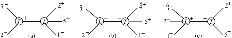
Figure 2: The recursive diagrams arising from a ${[3,4\rangle}$ shift in $A^{{\cal N}=0}_{5;1}(1^{-},2^{-},3^{-},4^{+},5^{+})$. Diagram (b) has a non-standard complex singularity.

Consider now the ${[3,4\rangle}$ shift,

$${\tilde{\lambda}}_{3}\rightarrow{\tilde{\lambda}}_{3}-z{\tilde{\lambda}}_{4}\,,\hskip 56.9055pt\lambda_{4}\rightarrow\lambda_{4}+z\lambda_{3}\,.$$ (21)

The three non-vanishing recursive diagrams are shown in fig. 2. These diagrams correspond to residues of the shifted amplitude at poles in $z$ where intermediate states go on shell. Diagrams 2(a) and 2(c) are straightforward to evaluate, because the three-point vertex is one which appears at tree level, and which can have only a single pole. Diagram 2(b), however, involves a one-loop “vertex” $A_{3}^{(1)}(2^{-},\hat{3}^{-};\hat{K}^{+})$. From refs. OnShellRecurrenceI ; Qpap , we know that the related “vertex”, with opposite intermediate helicity, $A_{3}^{(1)}(2^{-},\hat{3}^{-};\hat{K}^{-})$, does not factorize in complex momenta as a naive generalization of the factorization in real momenta. This property is related to the appearance of double poles at the loop level. In that case it was possible to deduce the relatively simple nonfactorizing structure, at least for the finite one-loop helicity amplitudes studied in refs. OnShellRecurrenceI ; Qpap . For the case of $A_{3}^{(1)}(2^{-},\hat{3}^{-};\hat{K}^{+})$, however, we do not know the general structure. Analysis of the behavior under shifting of $A^{{\cal N}=0}_{5;1}(1^{-},2^{-},3^{-},4^{+},5^{+})$ (see eq. (36) below), and of other known amplitudes, reveals that it is more subtle than the case of $A_{3}^{(1)}(2^{-},\hat{3}^{-};\hat{K}^{-})$. (It may even be that, in situations where double poles can appear, additional contributions arise which cannot be interpreted as factorized diagrams at all. However, an analysis of the diagrams such as those in fig. 2, which incorporates some empirical information about the non-standard terms, appears to cover any such additional contributions as well.)

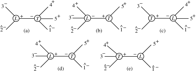
Figure 3: The recursive diagrams arising from a ${[1,2\rangle}$ shift in $A^{{\cal N}=0}_{5;1}(1^{-},2^{-},3^{-},4^{+},5^{+})$. As discussed in the text, only diagram (d) is nonvanishing.

Can we avoid diagrams like 2(b)? To study this, let us consider a ${[1,2\rangle}$ shift,

$${\tilde{\lambda}}_{1}\rightarrow{\tilde{\lambda}}_{1}-z{\tilde{\lambda}}_{2}\,,\hskip 56.9055pt\lambda_{2}\rightarrow\lambda_{2}+z\lambda_{1}\,,$$ (22)

which does in fact avoid generating diagrams whose complex factorization is as-yet unknown. The recursive diagrams for this shift are shown in fig. 3. (In the five-point case, choosing a ${[4,5\rangle}$ or ${[5,4\rangle}$ shift would avoid non-standard complex singularities, but as noted above its properties do not generalize simply to higher-point amplitudes.)

Before proceeding to inspect the specific diagrams in fig. 3, we make a few general remarks about the properties of three-point vertices, at one loop and beyond, which will be relevant for diagrams fig. 3(a) and fig. 3(e). Prior to assigning definite helicities to a three-point vertex with external legs $a$ and $b$, it can be written as $A_{3}^{\mu}(\varepsilon_{a},\varepsilon_{b})$, where $\varepsilon_{a},\varepsilon_{b}$ are the external polarization vectors, and $\mu$ is the Lorentz index for the intermediate gluon. This gluon is going on shell in a particular way; either $\left\langle a\,b\right\rangle$ or $\left[a\,b\right]$ is vanishing, depending on the choice of shift. Due to Bose symmetry, and the antisymmetry of the extracted color factor, $A_{3}^{\mu}(\varepsilon_{a},\varepsilon_{b})$ is antisymmetric under the exchange $k_{a}\leftrightarrow k_{b}$, $\varepsilon_{a}\leftrightarrow\varepsilon_{b}$. Using Bose symmetry and gauge invariance, there are only two possible terms in the tensor decomposition of $A_{3}^{\mu}(\varepsilon_{a},\varepsilon_{b})$ BDSSplit ; OneLoopSplitUnitarity ,

$$A_{3}^{\mu}(\varepsilon_{a},\varepsilon_{b}) = g_{1}(s_{ab},{\textstyle{k_{a}\cdot\eta\over(k_{a}+k_{b})\cdot\eta}})\,{1\over s_{ab}}\,(\varepsilon_{a}^{\mu}\,\varepsilon_{b}\cdot k_{a}-\varepsilon_{b}^{\mu}\,\varepsilon_{a}\cdot k_{b}+k_{b}^{\mu}\,\varepsilon_{a}\cdot\varepsilon_{b})$$ (23)

$$\hskip 0.0pt+\,g_{2}(s_{ab},{\textstyle{k_{a}\cdot\eta\over(k_{a}+k_{b})\cdot\eta}})\,k_{a}^{\mu}\,{1\over s_{ab}}\,\biggl{(}\varepsilon_{a}\cdot\varepsilon_{b}-{\varepsilon_{a}\cdot k_{b}\,\varepsilon_{b}\cdot k_{a}\over k_{a}\cdot k_{b}}\biggr{)}\,,$$

where the form factors $g_{1}$ and $g_{2}$ are symmetric under $k_{a}\leftrightarrow k_{b}$. (The required antisymmetry in $k_{a}\leftrightarrow k_{b}$ follows from the subleading nature of terms proportional to $K^{\mu}=-(k_{a}+k_{b})^{\mu}$.) We have introduced a fixed external vector $\eta$ to indicate that $g_{1}$ and $g_{2}$ may depend on how the intermediate gluon is going on shell. For example, in a real collinear limit, ${k_{a}\cdot\eta\over(k_{a}+k_{b})\cdot\eta}$ is the longitudinal momentum fraction carried by gluon $a$. The form factors can also depend on the vanishing quantity $s_{ab}$. However, the leading dependence can only be logarithmic, and so it is subdominant to the power-law behavior of the tensor structures.

The first tensor structure in eq. (23) is the one that appears at tree level,

$$A_{3}^{\rm tree,\,\mu}(\varepsilon_{a},\varepsilon_{b})={1\over s_{ab}}\,(\varepsilon_{a}^{\mu}\,\varepsilon_{b}\cdot k_{a}-\varepsilon_{b}^{\mu}\,\varepsilon_{a}\cdot k_{b}+k_{b}^{\mu}\,\varepsilon_{a}\cdot\varepsilon_{b})\,,$$ (24)

so we know a lot about its behavior in complex on-shell kinematics. The second tensor structure vanishes for opposite-helicity gluons; with reference vectors $q_{a}$ and $q_{b}$,

$$\varepsilon_{a}^{+}\cdot\varepsilon_{b}^{-}-{\varepsilon_{a}^{+}\cdot k_{b}\,\varepsilon_{b}^{-}\cdot k_{a}\over k_{a}\cdot k_{b}}=-{\left[a\,q_{b}\right]\left\langle b\,q_{a}\right\rangle\over\left\langle a\,q_{a}\right\rangle\left[b\,q_{b}\right]}+{\left[a\,b\right]\left\langle b\,q_{a}\right\rangle\left\langle b\,a\right\rangle\left[a\,q_{b}\right]\over\left\langle a\,q_{a}\right\rangle\left[b\,q_{b}\right]\left\langle a\,b\right\rangle\left[b\,a\right]}=0\,.$$ (25)

Therefore, in the case that the two external gluons have opposite helicity, if the tree-level vertex vanishes, the loop-level vertex (at any number of loops) should also vanish, since the same tensor structure is all that enters.

If the gluons have the same helicity, say both positive, the second tensor structure is nonvanishing off shell,

$$\varepsilon_{a}^{+}\cdot\varepsilon_{b}^{+}-{\varepsilon_{a}^{+}\cdot k_{b}\,\varepsilon_{b}^{+}\cdot k_{a}\over k_{a}\cdot k_{b}} = {\left[a\,b\right]\left\langle q_{b}\,q_{a}\right\rangle\over\left\langle a\,q_{a}\right\rangle\left\langle b\,q_{b}\right\rangle}-{\left[a\,b\right]\left\langle b\,q_{a}\right\rangle\left[b\,a\right]\left\langle a\,q_{b}\right\rangle\over\left\langle a\,q_{a}\right\rangle\left\langle b\,q_{b}\right\rangle\left\langle a\,b\right\rangle\left[b\,a\right]}$$ (26)

$$= -{\left[a\,b\right]\over\left\langle a\,b\right\rangle\left\langle a\,q_{a}\right\rangle\left\langle b\,q_{b}\right\rangle}(\left\langle a\,b\right\rangle\left\langle q_{a}\,q_{b}\right\rangle+\left\langle b\,q_{a}\right\rangle\left\langle a\,q_{b}\right\rangle)$$

$$= -{\left[a\,b\right]\over\left\langle a\,b\right\rangle}\,.$$

However, it vanishes if we approach the complex on-shell kinematics such that $\left[a\,b\right]\to 0$. Similarly, the structure relevant when both gluons have negative helicity vanishes as $\left\langle a\,b\right\rangle\to 0$. These configurations are those for which the corresponding tree-level vertices are also known to vanish. In summary, whenever a tree-level three-point vertex vanishes, the corresponding loop-level vertex should vanish as well.

Note that the identical-helicity tensor structure (26), which has a vanishing form factor $g_{2}$ at tree level, but not at one loop and beyond, has the form of an “unreal pole” Qpap ; that is, it is nonsingular for real collinear limits, but blows up or vanishes in complex on-shell kinematics. In the case that it blows up, the additional factor of $1/s_{ab}$ can produce a double pole in $\left\langle a\,b\right\rangle$, for the appropriate helicity of the intermediate gluon $P$. (The contraction $\varepsilon_{P}\cdot k_{a}$ is proportional to either $\left[a\,b\right]$ or $\left\langle a\,b\right\rangle$, depending on the helicity of $P$; the former case leads to the double pole.) The subleading terms in the expansion around such a double pole are non-standard, and are not yet understood. But again, this problem can occur only for the identical-helicity case, and only for the complex kinematical configuration for which the tree vertex is nonvanishing.

Now we return to the diagrams of fig. 3. First note that diagram 3(c) contains a tree-level vertex which vanishes in the complex on-shell kinematics, because

$$A_{3}^{\rm tree}(\hat{2}^{-},3^{-},-{\hat{K}}^{+}_{23})\propto\vphantom{\hat{K}}\left\langle\smash{\hat{2}}\,\smash{3}\right\rangle^{3}=0\,.$$ (27)

As a result, diagram 3(c) vanishes. Note that $A_{3}^{\rm tree}(\hat{2}^{-},3^{-},-{\hat{K}}^{+}_{23})$ would not have vanished with a shift of ${\tilde{\lambda}}_{2}$ instead of $\lambda_{2}$. From the above discussion, the loop vertex for the same helicity configuration and type of shift should also vanish. This vertex appears in diagram 3(a). Thus diagram 3(a) also vanishes. In the particular case at hand, we can easily verify that diagram 3(a) must vanish: If we examine the amplitude (19), we see that there is no pole in the $(23)$ channel. The reason is that only $\left[2\,3\right]$ products, not $\left\langle 2\,3\right\rangle$ products, are present in the denominators. The $\left[2\,3\right]$ products are left untouched by the ${[1,2\rangle}$ shift. Hence they cannot give rise to a pole in $z$ corresponding to diagram 3(a), which would be located at $\vphantom{\hat{K}}\left\langle\smash{\hat{2}}\,\smash{3}\right\rangle=0$, or $z=-\left\langle 2\,3\right\rangle/\left\langle 1\,3\right\rangle$.

Diagram 3(b) vanishes for the same reason as diagram 3(c). Diagram 3(e) contains a loop vertex with a configuration for which the corresponding tree vertex (which appears in diagram 3(d)) is nonvanishing. However, because it has opposite-helicity external gluons, we know that only the “standard” tree-type tensor structure in eq. (23) contributes. The one-loop form factor $g_{1}$ for the ${\cal N}=0$ case of a scalar in the loop can then be extracted from the one-loop splitting amplitude, and it vanishes. (In the notation of ref. Neq4Oneloop , $r_{S}^{[0]}(\lambda_{P},a^{\pm},b^{\mp})=0$, for either sign of $\lambda_{P}$.) In summary, all the recursive diagrams in fig. 3 are under control, and only diagram 3(d) is nonvanishing.

The ${[1,2\rangle}$ shift, however, fails to satisfy the second requirement that $A_{n}(z)\rightarrow 0$ as $z\rightarrow\infty$. For large $z$, we find that

$$A^{{\cal N}=0}_{5;1}(1^{-},2^{-},3^{-},4^{+},5^{+};z)\longrightarrow i\,{c_{\Gamma}\over 3}{\left\langle 1\,3\right\rangle^{3}\bigl{(}z\left\langle 1\,5\right\rangle+\left\langle 2\,5\right\rangle)\over\left\langle 1\,5\right\rangle^{2}\left\langle 3\,4\right\rangle\left\langle 4\,5\right\rangle\left[1\,2\right]}+{\cal O}\Bigl{(}{1\over z}\Bigr{)}\,.$$ (28)

It is easy to see that the following rational function has the same large-$z$ behavior as the full amplitude,

$$\mathop{\rm Inf}_{{[1,2\rangle}}{A^{{\cal N}=0}_{5;1}(1^{-},2^{-},3^{-},4^{+},5^{+})}=i\,{c_{\Gamma}\over 3}{\left\langle 1\,3\right\rangle^{3}\left\langle 2\,5\right\rangle\over\left\langle 1\,5\right\rangle^{2}\left\langle 3\,4\right\rangle\left\langle 4\,5\right\rangle\left[1\,2\right]}\,,$$ (29)

where $\mathop{\rm Inf}_{{[1,2\rangle}}{A}$ denotes those terms in $A$ that would give rise to a non-vanishing contribution upon performing a ${[1,2\rangle}$ shift and taking $z\rightarrow\infty$. (See section V.1 for further discussion of such terms.)

We note in contrast that $A^{{\cal N}=1}_{5;1}$ does vanish in the limit. More generally, supersymmetric loop amplitudes appear to vanish at large $z$ whenever the corresponding tree-level amplitudes do.

Based on our discussion, it is not surprising that with more positive-helicity gluons, higher-point ${\cal N}=0$ amplitudes in general suffer from one of these two problems (or perhaps both) under any shift: either a ‘bad’ channel with non-standard complex singularities, or ‘bad’ large-$z$ behavior.

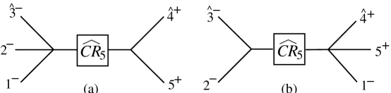
Figure 4: The overlap diagrams arising from an auxiliary ${[3,4\rangle}$ shift in $A^{{\cal N}=0}_{5;1}(1^{-},2^{-},3^{-},4^{+},5^{+})$.

III.3 Pairs of Shifts to the Rescue

To get around these problems, we use a combination of shifts, one particular shift to obtain one set of contributions, and a different shift to obtain the remaining contributions. In our five-point example, we take the ${[1,2\rangle}$ shift as the primary one for determining all terms except for the large-$z$ contributions given in eq. (29). We then use the ${[3,4\rangle}$ shift as an auxiliary shift for determining the large-$z$ contributions of the ${[1,2\rangle}$ shift. To see how this might be possible, imagine constructing the amplitude $A^{{\cal N}=0}_{5;1}(1^{-},2^{-},3^{-},4^{+},5^{+})$ via the auxiliary ${[3,4\rangle}$ shift

$${\tilde{\lambda}}_{3}\rightarrow{\tilde{\lambda}}_{3}-w{\tilde{\lambda}}_{4}\,,\hskip 56.9055pt\lambda_{4}\rightarrow\lambda_{4}+w\lambda_{3}\,,$$ (30)

where we have taken the shift parameter to be $w$, to distinguish it from the primary shift parameter in eq. (22). As above, we decompose the result into three pieces: the completed-cut terms, the overlap diagrams, and the recursive diagrams. Let us examine how each of these ${[3,4\rangle}$-decomposed pieces behaves under the action of the primary ${[1,2\rangle}$ shift, in particular as the parameter $z$ of that shift goes to infinity. To the recursive diagrams for the ${[3,4\rangle}$ shift shown in fig. 2, we add the overlap diagrams in fig. 4.

In computing the overlap diagrams in fig. 4, we choose a completed-cut expression based on eq. (19),

$${\widehat{C}}_{5}(1^{-},2^{-},3^{-},4^{+},5^{+}) =$$ (31)

$$\hskip-62.59605pt{1\over 3c_{\Gamma}}A^{{\cal N}=1}_{5;1}(1^{-},2^{-},3^{-},4^{+},5^{+})+{2\over 9}A^{{\rm tree}}_{5}(1^{-},2^{-},3^{-},4^{+},5^{+})$$

$$\hskip-62.59605pt\hbox{}+{i\over 3}{\left\langle 1\,2\right\rangle\left[2\,4\right]\left[5\,2\right]\left\langle 2\,3\right\rangle\biggl{(}\left[5\,1\right]\left\langle 1\,2\right\rangle\left[2\,4\right]+\left[5\,2\right]\left\langle 2\,3\right\rangle\left[3\,4\right]\biggr{)}\over\left[1\,2\right]\left[2\,3\right]}{\mathop{\rm L{}}\nolimits_{2a}\biggl{(}{-s_{34}\over-s_{51}}\biggr{)}\over s_{51}^{3}}\,,\hskip 14.22636pt$$

where we have kept the $2/9A_{5}^{\rm tree}$ term in the completed-cut term for consistency with our later computations. With this choice, it is a simple matter to check that under the ${[1,2\rangle}$ shift ${\widehat{C}}_{5}(z)$ vanishes for $z\rightarrow\infty$, using the ${\cal N}=1$ amplitude given in eq. (A), as well as eq. (18) for $\mathop{\rm L{}}\nolimits_{2a}(r)$.

Now consider the overlap contributions. These are obtained by extracting the residues of ${\widehat{CR}}_{5}(w)/w$, on the physical poles,

$$w^{\rm(a)}=-{\left\langle 4\,5\right\rangle\over\left\langle 3\,5\right\rangle}\,,\hskip 56.9055ptw^{\rm(b)}={\left[2\,3\right]\over\left[2\,4\right]}\,,$$ (32)

after applying the ${[3,4\rangle}$ shift. (The rational part of the completed-cut terms, ${\widehat{CR}}_{5}$, is obtained by setting all logarithms to zero in eq. (31).) The absence of a $\left\langle 4\,5\right\rangle$ product in the denominator of eq. (31) tells us that the first overlap contribution, fig. 4(a), vanishes. The other overlap contribution is straightforward to evaluate,

$$O^{\rm(b)} = -\biggl{(}{1\over 3\epsilon}+{8\over 9}\biggr{)}A^{{\rm tree}}_{5}(1^{-},2^{-},3^{-},4^{+},5^{+})$$

$$\hbox{}-{i\over 3}{\left\langle 1\,2\right\rangle\left[2\,4\right]\left[5\,2\right]\left\langle 2\,3\right\rangle\biggl{(}\left[5\,1\right]\left\langle 1\,2\right\rangle\left[2\,4\right]+\left[5\,2\right]\left\langle 2\,3\right\rangle\left[3\,4\right]\biggr{)}\over\left[1\,2\right]\left[2\,3\right]}\,{3s_{51}-s_{34}\over 2(s_{51}-s_{34})^{2}s_{51}^{2}}\,.$$

Applying a ${[1,2\rangle}$ shift to this expression and taking $z\rightarrow\infty$, we see that this expression also vanishes. This is, of course, not surprising, given that it is extracted from the completed-cut piece ${\widehat{C}}_{5}$, which vanishes at large $z$. Thus, there are no ${[1,2\rangle}$ large-$z$ contributions arising from cut or overlap terms.

This leaves us with the recursive diagrams to inspect. The first recursive diagram in fig. 2(a) is simple to evaluate, yielding,

$$D^{\rm(a)}=i\,\biggl{(}{1\over 3\epsilon}+{8\over 9}\biggr{)}{\left[4\,5\right]^{3}\over\left[1\,2\right]\left[1\,5\right]\left[2\,3\right]\left[3\,4\right]}\,.$$ (34)

The ${[1,2\rangle}$ shift of $D^{\rm(a)}$ clearly vanishes as $z\to\infty$.

While we do not know how to evaluate the second recursive diagram, we can nonetheless extract its value by ‘reverse engineering’ from the final answer. That is, we start from the final answer in eq. (19) (or equivalently, the form in eq. (A)), shift it, and extract the residue of $-A^{{\cal N}=0}_{5;1}(w)/w$ at $w=\left[2\,3\right]/\left[2\,4\right]$, with the logarithms set to zero. We find the contributions corresponding to the sum of diagrams 2(a) and 2(b). Subtracting off the value of diagram 2(a), eq. (34), gives us the reverse-engineered value for the non-standard residue encoded in diagram 2(b),

$$D^{\rm(b)} = {i\over 6}\Biggl{\{}-{\left\langle 1\,2\right\rangle\left\langle 2\,3\right\rangle\left[2\,4\right]\left[2\,5\right](s_{15}+s_{34})(\left\langle\smash{5}{\vphantom{1}}^{+}\right|{12}\left|\smash{4}{\vphantom{1}}^{-}\right\rangle+\left\langle\smash{5}{\vphantom{1}}^{+}\right|{23}\left|\smash{4}{\vphantom{1}}^{-}\right\rangle)\over\left\langle 1\,5\right\rangle\left\langle 3\,4\right\rangle\left[1\,2\right]\left[1\,5\right]\left[2\,3\right]\left[3\,4\right](s_{15}-s_{34})^{2}}$$ (35)

$$\hbox{}\hskip 17.07182pt+{\left\langle 1\,2\right\rangle\left\langle 2\,3\right\rangle\left[2\,4\right]\left[2\,5\right]\left[4\,5\right]\over\left[1\,2\right]\left[2\,3\right]s_{34}s_{15}}+2{\left\langle 1\,3\right\rangle^{2}\left\langle 1\,2\right\rangle\left[2\,4\right]\over\left[1\,2\right]\left[2\,3\right]\left\langle 3\,4\right\rangle\left\langle 5\,1\right\rangle^{2}}\Biggr{\}}\,.$$

Using some spinor-product identities, this result can be simplified to

$$D^{\rm(b)} = {i\over 3}{{\left\langle 1\,2\right\rangle}^{2}{\left[2\,4\right]}^{2}\left\langle 2\,3\right\rangle\over\left[1\,2\right]\left[2\,3\right]{\left\langle 5\,1\right\rangle}^{2}\ (s_{34}-s_{15})^{2}}\Bigl{(}2\left\langle 1\,5\right\rangle\left[5\,2\right]+{\left\langle 1\,3\right\rangle\over\left\langle 2\,3\right\rangle}(s_{34}-s_{15})\Bigr{)}\,.$$ (36)

The appearance of the unreal pole $\left\langle 2\,3\right\rangle/\left[2\,3\right]$ in this diagrammatic contribution is the hallmark of a non-standard factorization. If we now shift this expression under the primary ${[1,2\rangle}$ shift, and take the large-parameter limit, we see that both diagrams 2(a) and (b) vanish. In summary, the only piece of $A^{{\cal N}=0}_{5;1}(1^{-},2^{-},3^{-},4^{+},5^{+})$, decomposed according to the auxiliary ${[3,4\rangle}$ shift, which survives in the large-$z$ limit of the ${[1,2\rangle}$ shift, is that given by the ${[3,4\rangle}$ recursive diagram in fig. 2(c).

Therefore, while the ${[3,4\rangle}$ shift is not useful for evaluating the entire amplitude, because of the non-standard factorization in diagram 2(b), it is useful for deriving a recursion for those terms with bad large-$z$ behavior under a different shift. And once we have those terms, we can make use of the primary ${[1,2\rangle}$ shift to compute the entire amplitude.

Retaining only those terms from diagram 2(c) that contribute in the large-$z$ limit of the ${[1,2\rangle}$ shift, we find a remarkably simple recursion formula for these terms,

$$\mathop{\rm Inf}_{{[1,2\rangle}}{A^{{\cal N}=0}_{5;1}(1^{-},2^{-},3^{-},4^{+},5^{+})}=\mathop{\rm Inf}_{{[1,2\rangle}}{A^{{\cal N}=0}_{4;1}(1^{-},2^{-},\hat{3}^{-},\hat{K}_{45}^{+})}\times{i\over s_{45}}\times A_{3}^{\rm tree}(-\hat{K}_{45}^{-},\hat{4}^{+},5^{+})\,.$$ (37)

Here, we denote the operation of extracting the large-$z$ behavior of the ${[1,2\rangle}$ shift by $\mathop{\rm Inf}_{{[1,2\rangle}}{\mbox{}}$. We will give a formal definition of this operation in section V.1 below. In this recursion relation, $\hat{a}$ denotes a shifted momentum with the shift parameter frozen to the value,

$$w^{\rm(c)}=-{\left\langle 4\,5\right\rangle\over\left\langle 3\,5\right\rangle}\,,$$ (38)

according to the auxiliary ${[3,4\rangle}$ shift. The right-hand side of the recursion relation (37) simplifies, because both legs $1$ and $2$ that are shifted under the primary shift lie on one side of the pole, so only the first factor is affected by the extraction of the large-$z$ behavior.

To evaluate the recursion relation (37), we need the source of the large-$z$ behavior in the four-point amplitude, $A^{{\cal N}=0}_{4;1}(1^{-},2^{-},\hat{3}^{-},\hat{K}_{45}^{+})$, which may be obtained by relabeling the parity conjugate of eq. (168) in the appendix. We find,

$$\mathop{\rm Inf}_{{[1,2\rangle}}{A^{{\cal N}=0}_{5;1}(1^{-},2^{-},3^{-},4^{+},5^{+})} = -i\,{c_{\Gamma}\over 3}\,{\vphantom{\hat{K}}\left[\smash{1}\,\smash{\hat{3}}\right]\vphantom{\hat{K}}\left\langle\smash{1}\,\smash{\hat{3}}\right\rangle^{3}\over\vphantom{\hat{K}}\left\langle\smash{\hat{K}_{45}}\,\smash{1}\right\rangle\left[1\,2\right]\left[2\,\hat{3}\right]\vphantom{\hat{K}}\left\langle\smash{\hat{3}}\,\smash{\hat{K}_{45}}\right\rangle}\,{1\over s_{45}}\,{\vphantom{\hat{K}}\left[\smash{\hat{4}}\,\smash{5}\right]^{3}\over\vphantom{\hat{K}}\left[\smash{\hat{K}_{45}}\,\smash{\hat{4}}\right]\vphantom{\hat{K}}\left[\smash{5}\,\smash{\hat{K}_{45}}\right]}$$ (39)

$$= i\,{c_{\Gamma}\over 3}{\left\langle 1\,3\right\rangle^{3}\left\langle 2\,5\right\rangle\over\left\langle 1\,5\right\rangle^{2}\left\langle 3\,4\right\rangle\left\langle 4\,5\right\rangle\left[1\,2\right]}\,,$$

an expression identical to eq. (29). We see that the recursion relation (37), containing only the $(45)$ channel, reproduces the entire large-$z$ behavior of the five-point amplitude.

With this term in hand, we can compute the five-point amplitude using the ${[1,2\rangle}$ shift, even though the amplitude does not vanish as $z\rightarrow\infty$, because the difference $A^{{\cal N}=0}_{5;1}-\mathop{\rm Inf}_{{[1,2\rangle}}{A^{{\cal N}=0}_{5;1}}$ does have good behavior at infinity. The difference is given by the sum (17) of the completed-cut expression (31), the recursive diagrams (only diagram 3(d) is nonvanishing), and the overlap diagrams (only one is nonvanishing). This gives us a modified formula for the amplitude,

$$A_{n}=\mathop{\rm Inf}{A_{n}}+c_{\Gamma}\Bigl{[}{\widehat{C}}_{n}+R^{D}_{n}+O_{n}\Bigr{]}\,,$$ (40)

where the new term, $\mathop{\rm Inf}{A_{n}}$, accounts for a non-vanishing contribution at $z\rightarrow\infty$, compared to eq. (17). (We will need to modify this formula in subsequent sections to account for the possibility that the completed-cut terms also have nonvanishing large-$z$ behavior.)

III.4 Summary of Strategy

In summary, the above example suggests a simple strategy for constructing loop amplitudes, avoiding difficulties from either non-vanishing large-$z$ behavior or from non-standard complex factorizations:

• Use a primary shift whose recursion relation does not contain any non-standard complex factorizations, but under which the amplitude might not vanish at large $z$.

• Use an auxiliary shift and recursion relation to determine the large-$z$ behavior of the amplitude under the primary shift. This auxiliary recursion relation may contain non-standard complex factorizations, but these will be harmless if the contributions from these channels vanish in the large-$z$ limit of the primary shift.

In general, of course, we may not know ahead of time whether an amplitude has non-trivial large-parameter behavior for a chosen shift. We should therefore first derive an auxiliary recursion for this behavior (which might of course reveal that it is absent). The derivation of an auxiliary recursion relation may require assumptions about the behavior of contributions in ‘bad’ channels, such as that of the vanishing of diagram 2(b) in the large-parameter limit of the ${[1,2\rangle}$ shift. These assumptions can be verified once we have obtained a (candidate) final answer for the full amplitude, through a check of all (real-momentum) factorization limits. If the assumptions are not valid, and the auxiliary recursion relation yields an incomplete expression for the large-parameter behavior, the final answer will not have the correct collinear or multi-particle factorization limits. In section VI, we present shifts that we expect will satisfy all criteria necessary for constructing the rational parts of any $n$-gluon amplitude. We also expect this strategy to be widely applicable to other phenomenologically interesting amplitudes.

IV A Non-MHV Six-Point Example: $A_{6}(1^{-},2^{-},3^{-},4^{+},5^{+},6^{+})$

In the previous section we have developed a strategy for computing amplitudes even with shifts under which $A_{n}(z)\not\rightarrow 0$ as the shift parameter $z\rightarrow\infty$. We now apply these ideas to the calculation of a previously unknown amplitude with three negative helicities, $A^{{\cal N}=0}_{6;1}(1^{-},2^{-},3^{-},4^{+},5^{+},6^{+})$.

As in the five-point case, we shall use a ${[1,2\rangle}$ shift as the primary shift for computing the amplitude. For the same reasons as in the five-point case, the six-point amplitude is also free of contributions in ‘bad’ channels with non-standard complex singularities. So we can evaluate all of the recursive diagrams. It is clear from a consideration of the factorization properties as the momenta of gluons 5 and 6 become collinear that the amplitude must have non-trivial behavior at large $z$, because the corresponding five-point amplitude has such behavior under the shift. Our first task is to obtain a rational function which reproduces that behavior.

The full amplitude is obtained by combining the large-$z$ terms with the other standard terms — completed-cut terms, recursive diagrams, and overlap diagrams — via eq. (40). It turns out that we need to modify eq. (40) a bit more to subtract out nonvanishing large-$z$ contributions from the completed-cut terms, ${\widehat{C}}_{n}$. As we shall discuss more fully in section V, we are really performing a contour-integral analysis on the rational function of $z$, $(A_{n}(z)-[\mathop{\rm Inf}{A_{n}}](z))-{\widehat{C}}_{n}(z)$. It is this expression that must vanish as $z\to\infty$ to allow closing the contour at infinity. In the five-point example of the previous section, we avoided the need for subtracting the large-$z$ behavior of ${\widehat{C}}_{n}$, by use of the modified $\mathop{\rm L{}}\nolimits_{2}$ function in eq. (18); we simply ensured that ${{\widehat{C}}_{5}}(z)\to 0$ as $z\to\infty$. For more general amplitudes it is simpler to subtract out any nonvanishing large-$z$ contributions arising from ${\widehat{C}}_{n}$, before adding back the complete large-$z$ behavior. This amounts to performing a contour-integral analysis on $(A_{n}(z)-[\mathop{\rm Inf}{A_{n}}](z))-({\widehat{C}}_{n}(z)-[\mathop{\rm Inf}{{\widehat{C}}_{n}}](z))$, which automatically vanishes at infinity. The full result is then,

$$A_{n}=\mathop{\rm Inf}{A_{n}}+c_{\Gamma}\Bigl{[}{\widehat{C}}_{n}-\mathop{\rm Inf}{{\widehat{C}}_{n}}+R^{D}_{n}+O_{n}\Bigr{]}\,,$$ (41)

where $\mathop{\rm Inf}{A_{n}}$ contains the large-$z$ behavior of the entire amplitude, $R^{D}_{n}$ are the contributions from the recursive diagrams, and $O_{n}$ are the overlap pieces. In section V, we will provide a more systematic derivation of this formula.

IV.1 A Recursion Relation for Large-Parameter Behavior

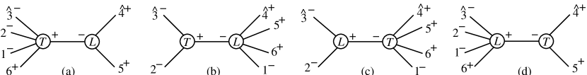
Figure 5: The recursive diagrams arising from an auxiliary ${[3,4\rangle}$ shift in $A^{{\cal N}=0}_{6;1}(1^{-},2^{-},3^{-},4^{+},5^{+},6^{+})$. Diagram (c) has non-standard complex singularities.

We begin by conjecturing a recursion relation for the large-$z$ behavior under the ${[1,2\rangle}$ shift that is the simplest possible generalization of the one we found for the five-point amplitude, namely,

$$\mathop{\rm Inf}_{{[1,2\rangle}}{A^{{\cal N}=0}_{6;1}(1^{-},2^{-},3^{-},4^{+},5^{+},6^{+})} = \mathop{\rm Inf}_{{[1,2\rangle}}{A^{{\cal N}=0}_{5;1}(1^{-},2^{-},\hat{3}^{-},\hat{K}_{45}^{+},6^{+})}\times{i\over s_{45}}$$ (42)

$$\hskip 56.9055pt\hbox{}\times A_{3}^{\rm tree}(-\hat{K}_{45}^{-},\hat{4}^{+},5^{+})\,.$$

As in eq. (37) for the five-point case, $\hat{a}$ indicates a momentum shifted according to the auxiliary ${[3,4\rangle}$ shift in eq. (30), with $w$ frozen to the value

$$w^{\rm(d)}=-{\left\langle 4\,5\right\rangle\over\left\langle 3\,5\right\rangle}\,.$$ (43)

We will return to a more systematic construction of the large-$z$ contributions via on-shell recursion in sections V-VII. Here we only wish to provide some motivation for the large-$z$ recursion relation (42), following the same procedure as at five points.

The recursive diagrams for computing the amplitude using a ${[3,4\rangle}$ shift are displayed in fig. 5. However, we are only interested in the values of the diagrams in the large-$z$ limit of the ${[1,2\rangle}$ shift. Diagram 5(a) has legs 1 and 2 attached to a tree which vanishes in the large-$z$ limit BCFW . As we shall discuss in section V.4, we assume, based on empirical evidence from known amplitudes, that the full diagram is also suppressed at large $z$, even though the loop vertex is non-standard. Diagram 5(b) is more complicated, in that the shifted legs straddle the pole, but its value may be determined easily since its components are known; it is then not difficult to verify that it is suppressed at large $z$. Diagram 5(c) is problematic, since it also contains a non-standard complex pole. For this case, we assume that the addition of the extra leg on the tree side, compared to the corresponding five-point diagram shown in fig. 2(b), does not upset the suppression at large $z$; we take it to have a vanishing contribution in this limit. One must also check that there are no additional large-$z$ contributions from the cut terms (after subtracting $\mathop{\rm Inf}{{\widehat{C}}_{n}}$) or from the overlap terms. Following a similar analysis as for the five-point case, it is not difficult to verify that there are none in this case. We are left with the single diagram 5(d), as the sole surviving contribution in the large-$z$ limit of the primary ${[1,2\rangle}$ shift, motivating eq. (42).

To evaluate the large-$z$ recursion relation in eq. (42), we use the five-point large-$z$ result in eq. (39) as input. We obtain,

$$\mathop{\rm Inf}_{{[1,2\rangle}}{A^{{\cal N}=0}_{6;1}(1^{-},2^{-},3^{-},4^{+},5^{+},6^{+})} = -i\,{c_{\Gamma}\over 3}{\vphantom{\hat{K}}\left\langle\smash{1}\,\smash{\hat{3}}\right\rangle^{3}\left\langle 2\,6\right\rangle\over\left\langle 1\,6\right\rangle^{2}\vphantom{\hat{K}}\left\langle\smash{\hat{3}}\,\smash{\hat{K}_{45}}\right\rangle\vphantom{\hat{K}}\left\langle\smash{\hat{K}_{45}}\,\smash{6}\right\rangle\left[1\,2\right]}\,{1\over s_{45}}\,{\vphantom{\hat{K}}\left[\smash{\hat{4}}\,\smash{5}\right]^{3}\over\vphantom{\hat{K}}\left[\smash{\hat{K}_{45}}\,\smash{\hat{4}}\right]\vphantom{\hat{K}}\left[\smash{5}\,\smash{\hat{K}_{45}}\right]}$$ (44)

$$= i\,{c_{\Gamma}\over 3}{\left\langle 1\,3\right\rangle^{3}\left\langle 2\,6\right\rangle\over\left\langle 1\,6\right\rangle^{2}\left\langle 3\,4\right\rangle\left\langle 4\,5\right\rangle\left\langle 5\,6\right\rangle\left[1\,2\right]}\,,$$

where, as above, $\hat{a}$ indicates a momentum shifted according to the ${[3,4\rangle}$ shift in eq. (30), with $w$ frozen to the value (43).

IV.2 The Completed-Cut Terms

The cut-containing terms of our target amplitude were computed in ref. RecurCoeff using a recursion relation on coefficients of integral functions, along with known lower-point results GGGGG ; Neq1Oneloop . In the six-point case, this procedure yields,

$${\widehat{C}}_{6}(1^{-},2^{-},3^{-},4^{+},5^{+},6^{+}) = \frac{1}{3c_{\Gamma}}\,A_{6;1}^{\,{\cal N}=1}(1^{-},2^{-},3^{-},4^{+},5^{+},6^{+})$$ (45)

$$\hskip 0.0pt+{2\over 9}A_{6}^{\rm tree}(1^{-},2^{-},3^{-},4^{+},5^{+},6^{+})+\hat{C}_{6}^{a}+\hat{C}_{6}^{a}\Bigr{|}_{\rm flip\;1}\,,~{}~{}$$

where

$$\hat{C}_{6}^{a} = {i\over 3}\Biggl{[}{\left\langle 1\,2\right\rangle\!\left\langle 2\,3\right\rangle\!\left[2\,4\right]\!\left\langle\smash{1}{\vphantom{1}}^{-}\right|{(3\!+\!4)}\left|\smash{2}{\vphantom{1}}^{-}\right\rangle\bigl{[}\left\langle\smash{3}{\vphantom{1}}^{-}\right|{42}\left|\smash{1}{\vphantom{1}}^{+}\right\rangle s_{234}-\left\langle\smash{3}{\vphantom{1}}^{-}\right|{2(3+4)}\left|\smash{1}{\vphantom{1}}^{+}\right\rangle s_{34}\bigr{]}\over\left\langle 3\,4\right\rangle\left\langle 5\,6\right\rangle\left\langle 6\,1\right\rangle\left[2\,3\right]\left\langle\smash{5}{\vphantom{1}}^{-}\right|{(3\!+\!4)}\left|\smash{2}{\vphantom{1}}^{-}\right\rangle}{\mathop{\hbox{\rm L}}\nolimits_{2}({-s_{234}\over-s_{34}})\over s_{34}^{3}}$$ (46)

$$\hskip 0.0pt+{\!\left\langle 3\,5\right\rangle\!\left[4\,5\right]\!\left[5\,6\right]\!\left\langle\smash{5}{\vphantom{1}}^{-}\right|{(1\!+\!2)}\left|\smash{6}{\vphantom{1}}^{-}\right\rangle\bigl{[}\left\langle\smash{3}{\vphantom{1}}^{-}\right|{(5-4)}\left|\smash{6}{\vphantom{1}}^{-}\right\rangle\!s_{345}+\left\langle\smash{3}{\vphantom{1}}^{-}\right|{(4+5)}\left|\smash{6}{\vphantom{1}}^{-}\right\rangle\!s_{34}\bigr{]}\,\over\left\langle 4\,5\right\rangle\left[1\,2\right]\left[1\,6\right]\left\langle\smash{5}{\vphantom{1}}^{-}\right|{(3+4)}\left|\smash{2}{\vphantom{1}}^{-}\right\rangle}{\mathop{\hbox{\rm L}}\nolimits_{2}({-s_{345}\over-s_{34}})\over s_{34}^{3}}\Biggr{]}\,,$$

and where we have introduced the flip symmetry operation,

$$X(1,2,3,4,5,6)\Bigr{|}_{\rm flip\;1}\equiv X(3,2,1,6,5,4)\,.$$ (47)

The first term in eq. (45) is proportional to the contribution of an ${\cal N}=1$ chiral multiplet in the loop. This contribution is fully constructible from the four-dimensional cuts Neq1Oneloop . The result is NeqOneNMHVSixPt ,

$$A_{6;1}^{\,{\cal N}=1}(1^{-},2^{-},3^{-},4^{+},5^{+},6^{+})=S_{6}^{a}+S_{6}^{a}\Bigr{|}_{\rm flip\;1}\,,$$ (48)

where

$$S_{6}^{a} = {ic_{\Gamma}\over 2}\Biggl{[}{1\over i}A_{6}^{\rm tree}(1^{-},2^{-},3^{-},4^{+},5^{+},6^{+})\,\mathop{\hbox{\rm K}}\nolimits_{0}(s_{34})$$

$$\hskip 19.91684pt-{\left\langle\smash{1}{\vphantom{1}}^{-}\right|{(2+3)}\left|\smash{4}{\vphantom{1}}^{-}\right\rangle^{2}\,\bigl{[}\left\langle\smash{3}{\vphantom{1}}^{-}\right|{42}\left|\smash{1}{\vphantom{1}}^{+}\right\rangle s_{234}-\left\langle\smash{3}{\vphantom{1}}^{-}\right|{2(3+4)}\left|\smash{1}{\vphantom{1}}^{+}\right\rangle s_{34}\bigr{]}\over\left\langle 5\,6\right\rangle\left\langle 6\,1\right\rangle\left[2\,3\right]\,s_{234}\,s_{34}\left\langle\smash{5}{\vphantom{1}}^{-}\right|{(3+4)}\left|\smash{2}{\vphantom{1}}^{-}\right\rangle}{\mathop{\hbox{\rm L}}\nolimits_{0}({-s_{234}\over-s_{34}})\over s_{34}}$$

$$\hskip 19.91684pt-{\left\langle\smash{3}{\vphantom{1}}^{-}\right|{(1+2)}\left|\smash{6}{\vphantom{1}}^{-}\right\rangle^{2}\bigl{[}\left\langle\smash{3}{\vphantom{1}}^{-}\right|{(5-4)}\left|\smash{6}{\vphantom{1}}^{-}\right\rangle s_{345}+\left\langle\smash{3}{\vphantom{1}}^{-}\right|{(4+5)}\left|\smash{6}{\vphantom{1}}^{-}\right\rangle s_{34}\bigr{]}\over\left\langle 3\,4\right\rangle\left\langle 4\,5\right\rangle\left[1\,2\right]\left[1\,6\right]\,s_{345}\,\left\langle\smash{5}{\vphantom{1}}^{-}\right|{(3+4)}\left|\smash{2}{\vphantom{1}}^{-}\right\rangle}{\mathop{\hbox{\rm L}}\nolimits_{0}({-s_{345}\over-s_{34}})\over s_{34}}\Biggr{]}\,.$$

After performing the ${[1,2\rangle}$ shift, the completed-cut expression given in eq. (45) does not vanish as $z\rightarrow\infty$, but tends to a purely-rational constant,

$$\mathop{\rm Inf}_{{[1,2\rangle}}{{\widehat{C}}_{6}(1^{-},2^{-},3^{-},4^{+},5^{+},6^{+})}=\lim_{z\rightarrow\infty}{\widehat{C}}_{6}(1^{-},2^{-},3^{-},4^{+},5^{+},6^{+};z)$$

$$\hskip 56.9055pt\hbox{}={i\over 6}{\left\langle 1\,2\right\rangle\left\langle 1\,3\right\rangle\left\langle\smash{3}{\vphantom{1}}^{-}\right|{(4+5)}\left|\smash{2}{\vphantom{1}}^{-}\right\rangle\Bigl{[}-\left\langle\smash{1}{\vphantom{1}}^{-}\right|{2(4+5)}\left|\smash{3}{\vphantom{1}}^{+}\right\rangle+\left\langle 1\,3\right\rangle s_{345}\Bigr{]}\over\left[1\,2\right]\left\langle 3\,4\right\rangle\left\langle 4\,5\right\rangle{\left\langle 6\,1\right\rangle}^{2}\,s_{345}\,\left\langle\smash{5}{\vphantom{1}}^{-}\right|{(3+4)}\left|\smash{2}{\vphantom{1}}^{-}\right\rangle}$$

$$\hskip 71.13188pt\hbox{}+{i\over 6}{\left\langle 1\,2\right\rangle\left[2\,4\right]\left\langle 1\,3\right\rangle(\left\langle 1\,2\right\rangle\left[2\,4\right]-\left\langle 1\,3\right\rangle\left[3\,4\right])\over\left[2\,3\right]\left\langle 5\,6\right\rangle\left\langle 6\,1\right\rangle\,s_{34}\,\left\langle\smash{5}{\vphantom{1}}^{-}\right|{(3+4)}\left|\smash{2}{\vphantom{1}}^{-}\right\rangle}\,.$$ (50)

Since we have already determined the complete large-$z$ behavior of the full amplitude in eq. (44), we must subtract from ${\widehat{C}}_{6}$ this rational constant, $\mathop{\rm Inf}_{{[1,2\rangle}}{{\widehat{C}}_{6}}$, so that the difference ${\widehat{C}}_{6}-\mathop{\rm Inf}_{{[1,2\rangle}}{{\widehat{C}}_{6}}$ vanishes as $z\rightarrow\infty$. When computing the overlap contribution we may use either this difference or the original ${\widehat{C}}_{6}$. They are equivalent because $\mathop{\rm Inf}_{{[1,2\rangle}}{{\widehat{C}}_{6}}$ has no poles in $z$ under a ${[1,2\rangle}$ shift; therefore it does not generate an overlap contribution.

IV.3 Recursive Contributions

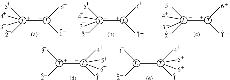
Figure 6: Some vanishing recursive diagrams for the ${[1,2\rangle}$ shift of $A^{{\cal N}=0}_{6;1}(1^{-},2^{-},3^{-},4^{+},5^{+},6^{+})$.

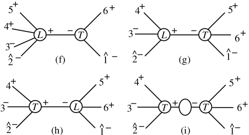
Figure 7: Non-vanishing recursive diagrams. Diagram (i) is the factorization-function contribution.

Next we evaluate the recursive diagrams for the ${[1,2\rangle}$ shift of $A^{{\cal N}=0}_{6;1}(1^{-},2^{-},3^{-},4^{+},5^{+},6^{+})$. Most of them vanish. Some of the vanishing diagrams are shown in fig. 6. (We omitted two diagrams in the $(23)$ channel, where $(-{\hat{K}}_{23})$ carries negative helicity, which vanish even more trivially.) The first two diagrams, 6(a) and 6(b), vanish because the loop vertices $R_{3}(6^{+},\hat{1}^{-},-\hat{K}_{61}^{\pm})$ vanish, as discussed in section III.2 and in the appendix. Diagrams 6(c) and 6(d) vanish because

$$A_{3}^{\rm tree}(6^{+},\hat{1}^{-},-{\hat{K}}_{61}^{+})\propto\vphantom{\hat{K}}\left[\smash{6}\,\smash{{\hat{K}}_{61}}\right]^{3}=0\,,\hskip 42.67912ptA_{3}^{\rm tree}(\hat{2}^{-},3^{-},-{\hat{K}}_{23}^{+})\propto\vphantom{\hat{K}}\left\langle\smash{\hat{2}}\,\smash{3}\right\rangle^{3}=0\,.$$ (51)

As discussed for the five-point case, diagram 6(e) vanishes because its loop vertex is of the same type as the vanishing tree vertex in diagram 6(d). Summarizing, we have

$$D_{6}^{\rm(a)}=D_{6}^{\rm(b)}=D_{6}^{\rm(c)}=D_{6}^{\rm(d)}=D_{6}^{\rm(e)}=0\,.$$ (52)

The four non-vanishing recursive diagrams,

$$R^{D}_{6}=D^{\rm(f)}+D^{\rm(g)}+D^{\rm(h)}+D^{\rm(i)}\,,$$ (53)

are shown in fig. 7. These diagrams are straightforward to evaluate because all channels involve standard factorizations. Diagram 7(f) yields

$$D_{6}^{\rm(f)} = A_{3}^{\rm tree}(\hat{1}^{-},-\hat{K}_{61}^{-},6^{+})\,{i\over s_{61}}\,R_{5}(\hat{2}^{-},3^{-},4^{+},5^{+},\hat{K}_{61}^{+})$$ (54)

$$= -i\biggl{(}{1\over 3\epsilon}+{8\over 9}\biggr{)}{{\left\langle\smash{3}{\vphantom{1}}^{-}\right|{(1+2)}\left|\smash{6}{\vphantom{1}}^{-}\right\rangle}^{3}\over\left[1\,2\right]\left\langle 3\,4\right\rangle\left\langle 4\,5\right\rangle\left[6\,1\right]\,s_{345}\,\left\langle\smash{5}{\vphantom{1}}^{-}\right|{(3+4)}\left|\smash{2}{\vphantom{1}}^{-}\right\rangle}$$

$$\hbox{}-{i\over 6}\,{s_{345}+s_{34}\over s_{34}s_{345}(s_{345}-s_{34})^{2}}{\left\langle 3\,5\right\rangle\left[4\,5\right]\left[5\,6\right]\left\langle\smash{5}{\vphantom{1}}^{-}\right|{(1+2)}\left|\smash{6}{\vphantom{1}}^{-}\right\rangle\over\left[1\,2\right]\left\langle 4\,5\right\rangle\left[6\,1\right]\,\left\langle\smash{5}{\vphantom{1}}^{-}\right|{(3+4)}\left|\smash{2}{\vphantom{1}}^{-}\right\rangle}$$

$$\hskip 28.45274pt\times(\left\langle\smash{3}{\vphantom{1}}^{-}\right|{4}\left|\smash{5}{\vphantom{1}}^{-}\right\rangle\left\langle\smash{5}{\vphantom{1}}^{-}\right|{(1+2)}\left|\smash{6}{\vphantom{1}}^{-}\right\rangle+\left\langle\smash{3}{\vphantom{1}}^{-}\right|{5}\left|\smash{6}{\vphantom{1}}^{-}\right\rangle s_{345})$$

$$\hbox{}+{i\over 3}\,{{\left[4\,6\right]}^{3}\left\langle\smash{4}{\vphantom{1}}^{-}\right|{(3+5)}\left|\smash{2}{\vphantom{1}}^{-}\right\rangle\over\left[1\,2\right]\left[2\,3\right]\left[3\,4\right]\left\langle 4\,5\right\rangle\left[6\,1\right]\,\left\langle\smash{5}{\vphantom{1}}^{-}\right|{(3+4)}\left|\smash{2}{\vphantom{1}}^{-}\right\rangle}+{i\over 3}\,{{\left[4\,6\right]}^{2}\left\langle\smash{3}{\vphantom{1}}^{-}\right|{(1+2)}\left|\smash{6}{\vphantom{1}}^{-}\right\rangle\over\left[1\,2\right]\left[3\,4\right]\left\langle 4\,5\right\rangle\left[6\,1\right]\,\left\langle\smash{5}{\vphantom{1}}^{-}\right|{(3+4)}\left|\smash{2}{\vphantom{1}}^{-}\right\rangle}$$

$$\hbox{}-{i\over 6}\,{\left\langle 3\,5\right\rangle\left[4\,5\right]\left[5\,6\right]\left\langle\smash{3}{\vphantom{1}}^{-}\right|{(1+2)}\left|\smash{6}{\vphantom{1}}^{-}\right\rangle\left\langle\smash{5}{\vphantom{1}}^{-}\right|{(1+2)}\left|\smash{6}{\vphantom{1}}^{-}\right\rangle\over\left[1\,2\right]\left\langle 4\,5\right\rangle\left[6\,1\right]\,s_{34}s_{345}\,\left\langle\smash{5}{\vphantom{1}}^{-}\right|{(3+4)}\left|\smash{2}{\vphantom{1}}^{-}\right\rangle}\,,$$

where the five-point scalar loop vertex is given in eq. (180). Diagram 7(g) is

$$D^{\rm(g)} = \,A_{4}^{\rm tree}(\hat{2}^{-},3^{-},4^{+},\hat{K}_{561}^{+})\,{i\over s_{561}}R_{4}(\hat{1}^{-},-\hat{K}_{561}^{-},5^{+},6^{+})$$ (55)

$$= \biggl{(}{1\over 3\epsilon}+{8\over 9}\biggr{)}A_{4}^{\rm tree}(\hat{2}^{-},3^{-},4^{+},\hat{K}_{561}^{+})\,{i\over s_{561}}\,A_{4}^{\rm tree}(\hat{1}^{-},-\hat{K}_{561}^{-},5^{+},6^{+})$$

$$= i\biggl{(}{1\over 3\epsilon}+{8\over 9}\biggr{)}{{\left\langle\smash{1}{\vphantom{1}}^{-}\right|{(2+3)}\left|\smash{4}{\vphantom{1}}^{-}\right\rangle}^{3}\over\left[2\,3\right]\left[3\,4\right]\left\langle 5\,6\right\rangle\left\langle 6\,1\right\rangle\,s_{234}\,\left\langle\smash{5}{\vphantom{1}}^{-}\right|{(3+4)}\left|\smash{2}{\vphantom{1}}^{-}\right\rangle}\,,$$

where we used the four-point tree amplitude, eq. (158), and the loop four-vertex given in eq. (175). It is easy to see that diagram 7(h) gives the same value,

$$D^{\rm(h)}=D^{\rm(g)}\,.$$ (56)

Diagram 7(i) contains the factorization function contribution BernChalmers , which for the scalar loop case amounts to a vacuum polarization insertion. The value of the factorization function vertex appearing in this diagram is given in eq. (166). Using this value of the factorization function, diagram 7(i) is given by

$$D^{\rm(i)} = -\biggl{(}{1\over 3\epsilon}+{8\over 9}\biggr{)}A_{4}^{\rm tree}(\hat{2}^{-},3^{-},4^{+},\hat{K}_{561}^{+})\,{i\over s_{561}}\,A_{4}^{\rm tree}(\hat{1}^{-},-\hat{K}_{561}^{-},5^{+},6^{+})$$ (57)

$$= -D^{\rm(g)}\,.$$

The fact that diagrams 7(g), (h) and (i) are equal, up to signs, is rather special to this amplitude.

IV.4 The Overlap Contributions

Figure 8: The overlap diagrams for the ${[1,2\rangle}$ shift. Diagram (a) vanishes.

To evaluate the overlap contributions we start from the rational parts of the completed-cut terms, obtained by setting all logarithms to zero in eq. (45). That is, we replace the $\mathop{\hbox{\rm K}}\nolimits_{0}$ and $\mathop{\rm L{}}\nolimits_{i}$ functions defined in eq. (171) with their rational parts,

$$\mathop{\hbox{\rm K}}\nolimits_{0}(r) \rightarrow {1\over\epsilon}+2\,,$$

$$\mathop{\rm L{}}\nolimits_{0}(r) \rightarrow 0\,,$$

$$\mathop{\rm L{}}\nolimits_{2}(r) \rightarrow {1\over 2}{(r+1)\over r(1-r)^{2}}\,.$$ (58)

Making these replacements in eq. (45) for ${\widehat{C}}_{6}$ gives us ${\widehat{CR}}_{6}$. Applying the ${[1,2\rangle}$ shift, eq. (22), yields ${\widehat{CR}}_{6}(z)$, which we use to evaluate the overlap contributions.

As depicted in fig. 8, for the ${[1,2\rangle}$ shift there are three channels which can potentially contribute to the overlap,

$$O=O^{\rm(a)}+O^{\rm(b)}+O^{\rm(c)}\,,$$ (59)

corresponding to the three residues of ${\widehat{CR}}_{6}(z)/z$ located at the values of $z$,

$$z^{\rm(a)}=-{\left\langle 2\,3\right\rangle\over\left\langle 1\,3\right\rangle}\,,\hskip 56.9055ptz^{\rm(b)}={\left[1\,6\right]\over\left[2\,6\right]}\,,\hskip 56.9055ptz^{\rm(c)}=-{s_{234}\over\left\langle\smash{1}{\vphantom{1}}^{-}\right|{(3+4)}\left|\smash{2}{\vphantom{1}}^{-}\right\rangle}\,.$$ (60)

Evaluating these residues gives us the overlap contributions. After simplification, they are given by,

$$O^{\rm(a)} = 0\,,$$

$$O^{\rm(b)} = i\biggl{(}{1\over 3\epsilon}+{8\over 9}\biggr{)}{{\left\langle\smash{3}{\vphantom{1}}^{-}\right|{(1+2)}\left|\smash{6}{\vphantom{1}}^{-}\right\rangle}^{3}\over\left[1\,2\right]\left\langle 3\,4\right\rangle\left\langle 4\,5\right\rangle\left[6\,1\right]\,s_{345}\,\left\langle\smash{5}{\vphantom{1}}^{-}\right|{(3+4)}\left|\smash{2}{\vphantom{1}}^{-}\right\rangle}$$

$$-{i\over 6}\,{\left\langle 1\,2\right\rangle\left\langle\smash{3}{\vphantom{1}}^{-}\right|{(4+5)}\left|\smash{2}{\vphantom{1}}^{-}\right\rangle{\left\langle\smash{3}{\vphantom{1}}^{-}\right|{(1+2)}\left|\smash{6}{\vphantom{1}}^{-}\right\rangle}^{2}\over\left[1\,2\right]\left\langle 3\,4\right\rangle\left\langle 4\,5\right\rangle\,s_{61}s_{345}\,\left\langle\smash{5}{\vphantom{1}}^{-}\right|{(3+4)}\left|\smash{2}{\vphantom{1}}^{-}\right\rangle}$$

$$+{i\over 6}\,{\left[4\,5\right]\left[5\,6\right]\left\langle 3\,5\right\rangle\left\langle\smash{5}{\vphantom{1}}^{-}\right|{(1+2)}\left|\smash{6}{\vphantom{1}}^{-}\right\rangle\left(\left\langle 3\,5\right\rangle\left[5\,6\right]s_{345}-\left\langle 3\,4\right\rangle\left[4\,5\right]\left\langle\smash{5}{\vphantom{1}}^{-}\right|{(3+4)}\left|\smash{6}{\vphantom{1}}^{-}\right\rangle\right)\over\left[1\,2\right]\left\langle 4\,5\right\rangle\left[6\,1\right]\left\langle\smash{5}{\vphantom{1}}^{-}\right|{(3+4)}\left|\smash{2}{\vphantom{1}}^{-}\right\rangle}$$

$$\quad\times{s_{34}+s_{345}\over s_{34}s_{345}\left(s_{345}-s_{34}\right)^{2}}$$

$$-{i\over 6}{\left\langle 1\,5\right\rangle\left[4\,5\right]\left[4\,6\right]\left\langle\smash{1}{\vphantom{1}}^{-}\right|{(5-6)}\left|\smash{4}{\vphantom{1}}^{-}\right\rangle\over\left[2\,3\right]\left[3\,4\right]\left\langle 5\,6\right\rangle s_{61}\left\langle\smash{5}{\vphantom{1}}^{-}\right|{(3+4)}\left|\smash{2}{\vphantom{1}}^{-}\right\rangle}\,,$$

$$O^{\rm(c)} = -i\biggl{(}{1\over 3\epsilon}+{8\over 9}\biggr{)}{{\left\langle\smash{1}{\vphantom{1}}^{-}\right|{(2+3)}\left|\smash{4}{\vphantom{1}}^{-}\right\rangle}^{3}\over\left[2\,3\right]\left[3\,4\right]\left\langle 5\,6\right\rangle\left\langle 6\,1\right\rangle\,s_{234}\,\left\langle\smash{5}{\vphantom{1}}^{-}\right|{(3+4)}\left|\smash{2}{\vphantom{1}}^{-}\right\rangle}$$ (61)

$$+{i\over 6}\,{\left\langle 1\,2\right\rangle\left[2\,4\right]{\left\langle\smash{1}{\vphantom{1}}^{-}\right|{(2+3)}\left|\smash{4}{\vphantom{1}}^{-}\right\rangle}^{2}\over\left[2\,3\right]\left[3\,4\right]\left\langle 5\,6\right\rangle\left\langle 6\,1\right\rangle\,s_{234}\,\left\langle\smash{5}{\vphantom{1}}^{-}\right|{(3+4)}\left|\smash{2}{\vphantom{1}}^{-}\right\rangle}$$

$$+{i\over 6}\,{\left\langle 1\,5\right\rangle\left\langle 3\,4\right\rangle\left[4\,5\right]\left\langle 1\,6\right\rangle{\left\langle\smash{1}{\vphantom{1}}^{-}\right|{(2+3)}\left|\smash{4}{\vphantom{1}}^{-}\right\rangle}^{2}\over\left[2\,3\right]\left\langle 5\,6\right\rangle{\left\langle 6\,1\right\rangle}^{2}\,s_{34}s_{234}\,\left\langle\smash{5}{\vphantom{1}}^{-}\right|{(3+4)}\left|\smash{2}{\vphantom{1}}^{-}\right\rangle}\,.$$

Although there is no need to keep the $1/\epsilon$ terms (their values are known a priori), we have carried them along.

IV.5 The Full Amplitude and Consistency Checks

We may now combine all the pieces to obtain the full amplitude,

$$A_{6;1}^{{\cal N}=0}(1^{-},2^{-},3^{-},4^{+},5^{+},6^{+})=c_{\Gamma}\Bigl{[}{\widehat{C}}_{6}+{\widehat{R}}_{6}\Bigr{]}\,,$$ (62)

where ${\widehat{C}}_{6}$ is given in eq. (45). The rational remainder ${\widehat{R}}_{6}$, consisting of recursive diagrams, overlap diagrams and large-$z$ contributions, is,

$${\widehat{R}}_{6} \equiv {1\over c_{\Gamma}}\mathop{\rm Inf}_{{[1,2\rangle}}{A_{6;1}^{{\cal N}=0}}-\mathop{\rm Inf}_{{[1,2\rangle}}{{\widehat{C}}_{6}}+D^{\rm(f)}+D^{\rm(g)}+D^{\rm(h)}+D^{\rm(i)}+O^{\rm(b)}+O^{\rm(c)}\,,$$ (63)

where $\mathop{\rm Inf}_{{[1,2\rangle}}{A_{6;1}^{{\cal N}=0}}$ is given in eq. (44) and $\mathop{\rm Inf}_{{[1,2\rangle}}{{\widehat{C}}_{6}}$ in eq. (50). The values of the recursive and overlap contributions are given in eqs. (54)–(57), and eq. (61). Simplifying the result for the rational remainder and making use of the flip symmetry (47), we can write the result for the remaining rational part in a rather compact form,

$${\widehat{R}}_{6}={\widehat{R}}_{6}^{a}+{\widehat{R}}^{a}_{6}\Bigr{|}_{\rm flip\;1}\,,$$ (64)

where

$${\widehat{R}}_{6}^{a} = {i\over 6}{1\over\left[2\,3\right]\left\langle 5\,6\right\rangle\,\left\langle\smash{5}{\vphantom{1}}^{-}\right|{(3+4)}\left|\smash{2}{\vphantom{1}}^{-}\right\rangle}\Biggl{\{}-{{\left[4\,6\right]}^{3}\left[2\,5\right]\left\langle 5\,6\right\rangle\over\left[1\,2\right]\left[3\,4\right]\left[6\,1\right]}-{{\left\langle 1\,3\right\rangle}^{3}\left\langle 2\,5\right\rangle\left[2\,3\right]\over\left\langle 3\,4\right\rangle\left\langle 4\,5\right\rangle\left\langle 6\,1\right\rangle}$$

$$\hskip 28.45274pt\hbox{}+{{\left\langle\smash{1}{\vphantom{1}}^{-}\right|{(2+3)}\left|\smash{4}{\vphantom{1}}^{-}\right\rangle}^{2}\over\left[3\,4\right]\left\langle 6\,1\right\rangle}\biggl{(}{\left\langle\smash{1}{\vphantom{1}}^{-}\right|{2}\left|\smash{4}{\vphantom{1}}^{-}\right\rangle-\left\langle\smash{1}{\vphantom{1}}^{-}\right|{5}\left|\smash{4}{\vphantom{1}}^{-}\right\rangle\over s_{234}}+{\left\langle 1\,3\right\rangle\over\left\langle 3\,4\right\rangle}-{\left[4\,6\right]\over\left[6\,1\right]}\biggl{)}$$

$$\hskip 28.45274pt\hbox{}-{{\left\langle 1\,3\right\rangle}^{2}(3\left\langle\smash{1}{\vphantom{1}}^{-}\right|{2}\left|\smash{4}{\vphantom{1}}^{-}\right\rangle+\left\langle\smash{1}{\vphantom{1}}^{-}\right|{3}\left|\smash{4}{\vphantom{1}}^{-}\right\rangle)\over\left\langle 3\,4\right\rangle\left\langle 6\,1\right\rangle}+{{\left[4\,6\right]}^{2}(3\left\langle\smash{1}{\vphantom{1}}^{-}\right|{5}\left|\smash{4}{\vphantom{1}}^{-}\right\rangle+\left\langle\smash{1}{\vphantom{1}}^{-}\right|{6}\left|\smash{4}{\vphantom{1}}^{-}\right\rangle)\over\left[3\,4\right]\left[6\,1\right]}\Biggr{\}}\,.\hskip 28.45274pt$$

The result (64) is manifestly symmetric, not only under the flip (47), but also under the second flip symmetry, involving spinor conjugation,

$$X(1,2,3,4,5,6)\Bigr{|}_{\rm flip\ 2}\equiv X^{*}(6,5,4,3,2,1).$$ (66)

The remarkable simplicity of the rational remainder is rather striking.

We have performed a number of checks on our result for the amplitude, eq. (62). We have confirmed that it has the proper factorization properties in real momenta in all two- and three-particle channels and that all spurious singularities indeed cancel as they should. Since the large-$z$ contribution in eq. (44) contains kinematic poles in a variety of channels, an omitted piece would necessarily be detected in some of the collinear limits. Finally, the numerical value at one phase-space point agrees with that in ref. EGZ06 . The consistency of the amplitude demonstrates the validity of our procedure for determining the large-$z$ terms, for a new and rather non-trivial analytic amplitude.

V On-Shell Recursion Relations for Loop Amplitudes

Before continuing to the case of general helicities, we present in this section a more systematic discussion of loop-level on-shell recursion relations, emphasizing the extensions beyond ref. Bootstrap . The derivation of such loop recursion relations is similar in spirit to the tree-level case, but it does require the treatment of factorizations which differ from the ‘ordinary’ factorization in real momenta. It also differs because of the appearance of branch cuts and spurious singularities associated with logarithms or polylogarithms. The cut-containing parts of the amplitude are an input to the loop recursion relations. We assume that they have been computed by other means, such as the unitarity-based method.

V.1 Analytic Behavior of Shifted Loop Amplitudes

The starting point for the loop recursion relations is a complex-valued shift of the momenta of a pair of external particles in an $n$-point amplitude, $k_{j}\to\hat{k}_{j}(z)$, $k_{l}\to\hat{k}_{l}(z)$. We describe a ${[j,l\rangle}$ shift in terms of the spinor variables $\lambda$ and ${\tilde{\lambda}}$ defined in eq. (3) ,

$${[j,l\rangle}:\hskip 56.9055pt{\tilde{\lambda}}_{j}\rightarrow{\tilde{\lambda}}_{j}-z{\tilde{\lambda}}_{l}\,,\hskip 56.9055pt\lambda_{l}\rightarrow\lambda_{l}+z\lambda_{j}\,,$$ (67)

following the tree-level construction BCFW . The shift maintains overall momentum conservation as well as the masslessness of the external momenta, $\hat{k}_{j}^{2}=\hat{k}_{l}^{2}=0$. Let us denote the original $n$-point amplitude by $A_{n}\equiv A_{n}(0)$, and the shifted one by $A_{n}(z)$. We seek an equation for $A_{n}(0)$ relying on the analytic properties of $A_{n}(z)$. (We will also denote by $f(z)$ other functions $f$ of the momenta, such as the cut-containing terms, after the shift (67).)

At tree level, $A_{n}(z)$ is a meromorphic function of $z$. Its poles are determined by the factorization properties of $A_{n}$ as multi-particle invariants or spinor products vanish. The former are identical for real and complex momenta, and at tree level, the singularities for spinor products of complex momenta are also completely determined by the corresponding singularities (collinear factorizations) for real momenta. At tree level, one can show BCFW ; GloverMassive ; VamanYao , that there are always choices of shift momenta for which $A_{n}(z)\rightarrow 0$ as $z\rightarrow\infty$. This allows the derivation of a recursion relation through consideration of a contour integral on a circle at infinity.

At one loop, we must consider several new aspects. The most obvious of these is the presence of branch cuts, which arise from logarithms or polylogarithms in the amplitudes. But there are a number of other important features. While factorization in real momenta is understood Neq4Oneloop ; BernChalmers ; OneLoopSplitUnitarity , this does not completely determine the singularity structure in complex momenta. In particular, we must in general handle double poles as well as ‘unreal’ poles, present for complex momenta but absent for real ones. We obtained some of the required factorizations heuristically OnShellRecurrenceI ; Qpap , confirming them by explicit calculation. In certain two-particle channels, however, the structure of complex factorization is not yet completely clear; accordingly, we will design our calculations to avoid relying on them.

While it does appear in general possible to find momentum shifts under which $A_{n}(z)\rightarrow 0$ as $z\rightarrow\infty$, it is not always possible to do so while avoiding poles in channels with obscure complex-factorization behavior. Accordingly, we must deal with amplitudes that have either a pole at infinity, so that $A_{n}(z)\rightarrow\infty$ as $z\rightarrow\infty$, or that behave as a finite constant. We will, however, assume that this behavior is given by a rational function of $z$. In all cases we deal with here, where the corresponding tree amplitudes vanish in the large-$z$ limit, the large-$z$ terms are purely rational. For the moment, let us assume we know these terms, along with the cut-containing terms; below we return to the issue of their computation.

More precisely, we wish to define an operator $\mathop{\rm Inf}{\hbox{}}$ that yields a pole-free rational function reproducing the large-$z$ behavior of an amplitude, when both are shifted,

$$\lim_{z\rightarrow\infty}\Bigl{(}\Bigl{[}\mathop{\rm Inf}{A_{n}}\Bigr{]}(z)-A_{n}(z)\Bigr{)}=0\,.$$ (68)

We implement this operator via a series expansion of the amplitude around the point $z=\infty$, or $u=1/z=0$. We take $A_{n}(z)$ to be an analytic function with a series expansion of the form,

$$A_{n}(z)=\sum_{i=0}^{i_{\rm max}}{1\over u^{i}}\,a^{(-i)}+\sum_{i=1}^{\infty}u^{i}\,b^{(i)}+\sum_{i=1}^{\infty}\ln(u)u^{i}\,c^{(i)}+\sum_{i=1}^{\infty}\ln^{2}(u)u^{i}\,d^{(i)}\,,$$ (69)

where the coefficients, $a^{(-i)}$, $b^{(i)}$, $c^{(i)}$ and $d^{(i)}$ depend on spinor products. The leading degree of large-$z$ behavior, $i_{\rm max}$, depends on the helicity configuration. In writing this expansion, we have assumed that no $\ln(z)$ factors appear in terms which survive as $z\rightarrow\infty$. (We can always confirm the validity of this assumption for a given amplitude, since all logs and polylogarithms will have already been computed via the unitarity method or other means.) The large-$z$ terms are those which do not vanish as $z\rightarrow\infty$,

$$A^{{{\rm lrg\ }z}}_{n}(z)\equiv\sum_{i=0}^{i_{\rm max}}z^{i}\,a^{(-i)}=\Big{[}\mathop{\rm Inf}A_{n}\Big{]}(z)\,,$$ (70)

given by shifting their progenitor $\mathop{\rm Inf}A_{n}$.

We may then write $A_{n}(z)$ as a sum of the large-$z$ terms and the remaining terms,

$$A_{n}(z)=A^{{{\rm lrg\ }z}}_{n}(z)+A^{\rm poles}_{n}(z)\,,$$ (71)

so that all finite-$z$ poles, logarithms, and polylogarithms in $z$ are put in the second term. We will call the latter object the ‘finite-pole’ terms.

Since we will be interested in the unshifted physical amplitude obtained by setting $z=0$, we will need those terms in $A_{n}(0)$ that generate $A^{{{\rm lrg\ }z}}_{n}(z)$ under the shift. We find in practice that these are given by setting $z=0$ in $A^{{{\rm lrg\ }z}}_{n}(z)$, that is keeping only the $z^{0}=u^{0}$ terms in the expansion of $A_{n}(z)$,

$$\mathop{\rm Inf}{A_{n}}=a^{(0)}\,.$$ (72)

A key aim of this paper is to provide a means for computing this quantity.

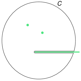
Figure 9: A configuration of poles and branch cuts for a term in a one-loop amplitude, with a branch-cut-hugging contour.

Since $A^{\rm poles}_{n}(z)$ vanishes for $z\rightarrow\infty$, we may apply Cauchy’s residue theorem. Consider the contour going along the circle at infinity, but avoiding the branch cuts by integrating inwards along one side, and then outwards along the other, as shown in fig. 9. We route the branch cuts so that no two overlap. (As discussed in ref. Bootstrap the case of poles touching the ends of branch cuts works in the same way as the basic case, and we shall not distinguish it further in our discussion.) The integral along this contour is given by the sum of residues. This contour, however, includes a branch-cut-hugging integral,

$${1\over 2\pi i}\int_{B^{\uparrow}+i\epsilon}{dz\over z}\;A^{\rm poles}_{n}(z)+{1\over 2\pi i}\int_{B^{\downarrow}-i\epsilon}{dz\over z}\;A^{\rm poles}_{n}(z)\,,$$ (73)

where $B^{\uparrow}$ is directed from an endpoint $B_{0}$ to infinity, and $B^{\downarrow}$ is directed in the opposite way. Now, $A^{\rm poles}_{n}(z)$ has a branch cut along $B$, which means that it has a non-vanishing discontinuity,

$$2\pi i\mathop{\rm Disc}\nolimits_{B}A^{\rm poles}_{n}(z)=A^{\rm poles}_{n}(z+i\epsilon)-A^{\rm poles}_{n}(z-i\epsilon),\qquad z{\rm\ on\ }B\,.$$ (74)

(Because $A^{{{\rm lrg\ }z}}_{n}$ is taken to be purely rational, $\mathop{\rm Disc}\nolimits_{B}A^{\rm poles}_{n}(z)=\mathop{\rm Disc}\nolimits_{B}A_{n}(z)$.) Thus, using the vanishing of $A^{\rm poles}_{n}(z)$ for $z\rightarrow\infty$, we have,

$$0=A^{\rm poles}_{n}(0)+\sum_{{\rm poles}\ \alpha}\mathop{\rm Res}_{z=z_{\alpha}}{A^{\rm poles}_{n}(z)\over z}+\int_{B_{0}}^{\infty}{dz\over z}\;\mathop{\rm Disc}\nolimits_{B}A^{\rm poles}_{n}(z)\,.$$ (75)

V.2 Cuts and Cut Completion

To proceed further, let us assume that we have already computed all terms having branch cuts, along with certain closely related terms that can generally be obtained from the same computation. That is, we have computed all polylog terms, all log terms, and all $\pi^{2}$ terms. As discussed in ref. Bootstrap , there are also certain classes of rational terms that are natural to include with the cut-containing terms.

In particular, there are rational terms whose presence is required to cancel spurious singularities in the (poly)logarithmic terms. Such spurious singularities arise in the course of integral reductions. They are not singularities of the final amplitude, because they are unphysical, and not singularities of any Feynman diagram. A simple example comes from a ‘two-mass’ triangle integral for which two of the three external legs are off shell (massive), with momentum invariants $s_{1}$ and $s_{2}$, say. When there are sufficiently many loop momenta inserted in the numerator of this integral, it gives rise to functions such as,

$${\ln(r)\over(1-r)^{2}}\,,$$ (76)

where $r$ is a ratio of momentum invariants (here $r=s_{1}/s_{2}$). The limit $r\rightarrow 1$ (that is, $s_{1}\rightarrow s_{2}$) is a spurious singularity; it does not correspond to any physical factorization. Indeed, this function always appears in the amplitude together with appropriate rational pieces,

$${\ln(r)+1-r\over(1-r)^{2}}\,,$$ (77)

in a combination which is finite as $r\rightarrow 1$. From a practical point of view, it is most convenient to ‘complete’ the unitarity-derived answer for the cuts by replacing functions like eq. (76) with non-singular combinations like eq. (77). Such completions are of course not unique; one could add additional rational terms free of spurious singularities.

The reason we want to eliminate spurious singularities from sub-expressions has to do with the sum over pole residues in eq. (75). The sum runs over all poles, whether they arise from a shift in a physical singularity variable, or in a spurious one. In practice, it is sufficient to eliminate all spurious singularities that acquire a $z$ dependence under the momentum shift. By construction, $A^{{{\rm lrg\ }z}}_{n}(z)$ is free of such ‘dangerous’ spurious singularities, since it cannot contain poles in $z$.

Singularities that look like collinear ones, but involve non-adjacent momenta, are also spurious. For example, in the scalar contributions to the five-gluon $({-}{+}{-}{+}{+})$ amplitude GGGGG , there are factors of $\left\langle 2\,4\right\rangle$ and $\left\langle 2\,5\right\rangle$ appearing in the denominators of certain coefficients. These might appear to give rise to non-adjacent collinear singularities in complex momenta; but by expanding the polylogarithms and logarithms in that limit, one can show that these singularities are in fact absent in the full amplitude.

Let us define two decompositions of the amplitude. The first is into ‘pure-cut’ and ‘rational’ pieces. The rational parts are defined by setting all logarithms, polylogarithms, and $\pi^{2}$ terms to zero,

$$R_{n}(z)\equiv{1\over c_{\Gamma}}A_{n}\Bigr{|}_{\rm rat}={1\over c_{\Gamma}}A_{n}\biggr{|}_{\ln,\mathop{\rm Li}\nolimits,\pi^{2}\rightarrow 0}\,.$$ (78)

(The normalization constant $c_{\Gamma}$, defined in eq. (15), plays no essential role in the following arguments, we carry it along for completeness.) The ‘pure-cut’ terms are the remaining terms, all of which must contain logarithms, polylogarithms, or $\pi^{2}$ terms,

$$C_{n}(z)\equiv{1\over c_{\Gamma}}A_{n}\Bigr{|}_{\rm pure-cut}={1\over c_{\Gamma}}A_{n}\biggr{|}_{\ln,\mathop{\rm Li}\nolimits,\pi^{2}}\,.$$ (79)

In other words,

$$A_{n}(z)=c_{\Gamma}\Bigl{[}C_{n}(z)+R_{n}(z)\Bigr{]}\,,$$ (80)

where we have explicitly taken $c_{\Gamma}$ outside of $C_{n}(z)$ and $R_{n}(z)$.

The second decomposition uses the ‘completed-cut’ terms, obtained from $C_{n}(z)$ by replacing logarithms and polylogarithms by corresponding functions free of spurious singularities (at least those that suffer a shift). We call this completion ${\widehat{C}}_{n}$. The decomposition defines the remaining rational pieces ${\widehat{R}}_{n}$,

$$A_{n}(z)=c_{\Gamma}\Bigl{[}{\widehat{C}}_{n}(z)+{\widehat{R}}_{n}(z)\Bigr{]}\,.$$ (81)

This reorganization has effectively moved some of the rational terms into the completed-cut terms. In general, $C_{n}(z)$ and ${\widehat{C}}_{n}(z)$ will not vanish as $z\rightarrow\infty$. We will assume that the large-$z$ behavior is given by a rational function of the spinor products, as in the previous examples. The rational function may include contributions from series expansions of the logarithms and polylogarithms in ${\widehat{C}}_{n}(z)$. Taking this into account, we can define a useful decomposition of the finite-pole terms,

$$A^{\rm poles}_{n}(z)=c_{\Gamma}\Bigl{[}{\widehat{C}}_{n}(z)+{\widehat{R}}_{n}(z)-[\mathop{\rm Inf}{\widehat{C}}_{n}](z)-[\mathop{\rm Inf}{\widehat{R}}_{n}](z)\Bigr{]}\,.$$ (82)

In the cases relevant to the present paper, $[\mathop{\rm Inf}{\widehat{C}}_{n}](z)$ is in fact at worst a constant in $z$. Note that the additional terms will not contain any ‘dangerous’ spurious singularities, as the act of taking the large-$z$ limit will eliminate them.

We also need to define the rational part of the completed-cut terms, $\widehat{CR}_{n}(z)$. We write,

$${\widehat{C}}_{n}(z)=C_{n}(z)+{\widehat{CR}}_{n}(z)\,,$$ (83)

where

$${\widehat{CR}}_{n}(z)\equiv{\widehat{C}}_{n}(z)\Bigr{|}_{\rm rat}\,.$$ (84)

Combining eqs. (80), (81), and (83), we see that the full rational part is the sum of the rational part of the completed-cut terms, and the remaining rational pieces,

$$R_{n}(z)={\widehat{CR}}_{n}(z)+{\widehat{R}}_{n}(z)\,.$$ (85)

Now, because we know all the terms containing branch cuts, we could compute the branch-cut-hugging integral in eq. (75),

$$\int_{B_{0}}^{\infty}{dz\over z}\;\mathop{\rm Disc}\nolimits_{B}A^{\rm poles}_{n}(z) = \int_{B_{0}}^{\infty}{dz\over z}\;\mathop{\rm Disc}\nolimits_{B}\bigl{[}{\widehat{C}}_{n}(z)-[\mathop{\rm Inf}{\widehat{C}}_{n}](z)\bigr{]}$$ (86)

$$= \int_{B_{0}}^{\infty}{dz\over z}\;\mathop{\rm Disc}\nolimits_{B}{\widehat{C}}_{n}(z)\,,$$

where the second line follows from the rational nature of $[\mathop{\rm Inf}{\widehat{C}}_{n}](z)$. However, there is no need to do the integral explicitly, because we already know the answer for the integral, plus the associated residues. Up to a contribution coming from $\mathop{\rm Inf}{\widehat{C}}_{n}$, it is just ${\widehat{C}}_{n}(0)$, part of the final answer. That is, applying the same logic to ${\widehat{C}}_{n}(z)-[\mathop{\rm Inf}{\widehat{C}}_{n}](z)$ as was applied to $A^{\rm poles}_{n}(z)$ in eq. (75), we have,

$${\widehat{C}}_{n}(0)=\mathop{\rm Inf}{\widehat{C}}_{n}-\sum_{{\rm poles}\ \alpha}\mathop{\rm Res}_{z=z_{\alpha}}{{\widehat{C}}_{n}(z)\over z}-\int_{B_{0}}^{\infty}{dz\over z}\;\mathop{\rm Disc}\nolimits_{B}{\widehat{C}}_{n}(z)\,,$$ (87)

where by construction $\mathop{\rm Inf}{\widehat{C}}_{n}$ does not contribute to the sum over residues either.

Using eq. (75), the decomposition (81), and eq. (87) to evaluate the terms involving ${\widehat{C}}_{n}(z)$, we can write our desired answer as follows,

$$A^{\rm poles}_{n}(0) = -c_{\Gamma}\Biggl{[}\int_{B_{0}}^{\infty}{dz\over z}\;\mathop{\rm Disc}\nolimits_{B}{\widehat{C}}_{n}(z)+\sum_{{\rm poles}\,\alpha}\mathop{\rm Res}_{z=z_{\alpha}}{{\widehat{C}}_{n}(z)\over z}+\sum_{{\rm poles}\,\alpha}\mathop{\rm Res}_{z=z_{\alpha}}{{\widehat{R}}_{n}(z)\over z}\Biggr{]}$$ (88)

$$= c_{\Gamma}\Biggl{[}{\widehat{C}}_{n}(0)-\mathop{\rm Inf}{\widehat{C}}_{n}-\sum_{{\rm poles}\,\alpha}\mathop{\rm Res}_{z=z_{\alpha}}{{\widehat{R}}_{n}(z)\over z}\Biggr{]}\,.$$

By construction, the completed-cut terms ${\widehat{C}}_{n}(z)$ contain no spurious singularities, and so the sums over the poles in eq. (88) are only over the genuine, ‘physical’ poles in the amplitude. As we are working with complex momenta, these are the poles that arise for such momenta, and not merely those that arise for real momenta. In particular, this means that double poles and unreal poles may appear, as discussed in detail in refs. OnShellRecurrenceI ; Qpap .

V.3 Residues of the Remaining Rational Pieces ${\widehat{R}}_{n}(z)$

Our next task is to evaluate the residues of the remaining rational terms, ${\widehat{R}}_{n}$. We will do this by setting up an on-shell recursion relation. As discussed in ref. Bootstrap , pure-cut and rational terms factorize independently, and so one can use factorization to construct an on-shell recursion relation for the full rational terms $R_{n}$. However, there is no fundamental factorization distinction between the rational terms in ${\widehat{C}}_{n}$ and those in ${\widehat{R}}_{n}$, so we cannot set up a direct recursion relation for them. We will instead compute them indirectly, by first computing the full rational terms, and then subtracting terms which are present in both the full rational terms and in the completed-cut terms. These are exactly terms coming from ${\widehat{CR}}_{n}$, which we therefore call ‘overlap’ terms,

$$-\sum_{{\rm poles}\,\alpha}\mathop{\rm Res}_{z=z_{\alpha}}{{\widehat{R}}_{n}(z)\over z}=-\sum_{{\rm poles}\,\alpha}\mathop{\rm Res}_{z=z_{\alpha}}{R_{n}(z)\over z}+\sum_{{\rm poles}\,\alpha}\mathop{\rm Res}_{z=z_{\alpha}}{{\widehat{CR}}_{n}(z)\over z}\,.$$ (89)

Since we know ${\widehat{CR}}_{n}$ explicitly, we can compute the last sum by shifting and extracting poles,

$$O_{n}\equiv\sum_{{\rm poles}\,\alpha}\mathop{\rm Res}_{z=z_{\alpha}}{{\widehat{CR}}_{n}(z)\over z}\,.$$ (90)

To obtain the first term on the right-hand side of eq. (89), we must analyze the poles in $R_{n}(z)$, that is to say its properties at appropriate null complex momenta. The behavior of $R_{n}(z)$ can be extracted from the factorization properties of the amplitude as a whole, by following the analysis of ref. Bootstrap , and separating two classes of terms — pure-cut and rational — in the factorized amplitudes. Only rational terms in the factorization can contribute to the required sum of residues.

Given the ${[j,l\rangle}$ shift (67), we define a partition $P$ to be a set of two or more cyclicly-consecutive momentum labels containing $j$, such that the complementary set ${\overline{P}}$ consists of two or more cyclicly-consecutive labels containing $l$:

$$P \equiv \{P_{1},P_{2},\ldots,j,\ldots,P_{-1}\}\,,$$ (91)

$${\overline{P}} \equiv \{{\overline{P}}_{1},{\overline{P}}_{2},\ldots,l,\ldots,{\overline{P}}_{-1}\}\,,$$

$$P \cup {\overline{P}}=\{1,2,\ldots,n\}\,.$$

This definition ensures that the sum of momenta in each partition is $z$-dependent, so that it can go on shell for a suitable value of $z$. The complex on-shell momenta $\hat{k}_{j}$, $\hat{k}_{l}$ and ${\hat{P}}$ are determined by solving the on-shell condition, ${\hat{P}}^{2}=0$, for $z$.

At one loop, there are in general three contributions to factorization in any given channel,

$$A^{1\mbox{-}\rm loop}\Bigl{|}_{s_{i\ldots j}}=A_{L}^{1\mbox{-}\rm loop}\times{i\over s_{i\ldots j}}\times A_{R}^{\rm tree}+A_{L}^{\rm tree}\times{i\over s_{i\ldots j}}\times A_{R}^{1\mbox{-}\rm loop}+A_{L}^{\rm tree}\times{i\,{\cal F}^{1\mbox{-}\rm loop}\over s_{i\ldots j}}\times A_{R}^{\rm tree}\,.$$ (92)

In the first two terms, one of the factorized amplitudes is a one-loop amplitude and the other is a tree amplitude. The last term contributes only in multi-particle channels, and contains a one-loop ‘factorization function’. For the case of a scalar in the loop (${\cal N}=0$), this function is equal to the scalar contribution to the gluon vacuum polarization BernChalmers . Accordingly, in addition to the sum over channels, we will have a sum over these different factorization contributions. Taking the rational parts, we obtain,

$$-\sum_{{\rm poles}\ \alpha}\mathop{\rm Res}_{z=z_{\alpha}}{R_{n}(z)\over z} \equiv R^{D}_{n}(k_{1},\ldots,k_{n})$$

$$= \hskip-2.84544pt\sum_{{\rm partitions}\,P}\,\sum_{h=\pm}\Biggl{\{}R(k_{P_{1}},\ldots,\hat{k}_{j},\ldots,k_{P_{-1}},-{\hat{P}}^{h})$$

$$\hbox{}\hskip 71.13188pt\hskip 19.91692pt\times{i\over P^{2}}\times A^{\rm tree}(k_{{\overline{P}}_{1}},\ldots,\hat{k}_{l},\ldots,k_{{\overline{P}}_{-1}},{\hat{P}}^{-h})$$

$$\hbox{}\hskip 71.13188pt+A^{\rm tree}(k_{P_{1}},\ldots,\hat{k}_{j},\ldots,k_{P_{-1}},-{\hat{P}}^{h})$$

$$\hbox{}\hskip 71.13188pt\hskip 19.91692pt\times{i\over P^{2}}\times R(k_{{\overline{P}}_{1}},\ldots,\hat{k}_{l},\ldots,k_{{\overline{P}}_{-1}},{\hat{P}}^{-h})$$

$$\hbox{}\hskip 71.13188pt+A^{\rm tree}(k_{P_{1}},\ldots,\hat{k}_{j},\ldots,k_{P_{-1}},-{\hat{P}}^{h})$$

$$\hbox{}\hskip 71.13188pt\hskip 19.91692pt\times{iR_{\cal F}(P)\over P^{2}}\times A^{\rm tree}(k_{{\overline{P}}_{1}},\ldots,\hat{k}_{l},\ldots,k_{{\overline{P}}_{-1}},{\hat{P}}^{-h})\Biggr{\}}\,,$$

where $P^{2}$ is the squared momentum associated with the partition $P$, and $R_{\cal F}$ is defined in the appendix. The hatted variables are given as usual by shifting momenta according to eq. (67), and freezing $z$ to the value that puts $\hat{P}$ on shell,

$$z={P^{2}\over\langle j^{-}|P|l^{-}\rangle}\,.$$ (94)

The result (V.3) follows directly from the general factorization behavior of one-loop amplitudes, plus the separate factorization of pure-cut and rational terms Bootstrap . Although the $R$ functions are not complete amplitudes, they can be thought of as vertices. Equation (V.3) then gives rise to a set of ‘recursive diagrams’.

Inserting the result into eq. (88), and thence into eq. (71), gives us the basic on-shell recursion relation for complete one-loop amplitudes,

$$A_{n}(0)=\mathop{\rm Inf}{A_{n}}+c_{\Gamma}\biggl{[}{\widehat{C}}_{n}(0)-\mathop{\rm Inf}{{\widehat{C}}_{n}}+R^{D}_{n}+O_{n}\biggr{]}\,.$$ (95)

To compute with this equation, we construct $R^{D}_{n}$ via recursive diagrams; that is, via eq. (V.3). The ‘overlap’ terms $O_{n}$ can also be given a diagrammatic interpretation, associating each pole in eq. (90) with a specific diagram, as we have done in figs. 4 and 8. Although the definition of the completed-cut terms ${\widehat{C}}_{n}$ is not unique, the ambiguity cancels between ${\widehat{C}}_{n}(0)$, $\mathop{\rm Inf}{{\widehat{C}}_{n}}$, and the sum over ${\widehat{CR}}_{n}$ residues in $O_{n}$.

In general, it is useful to combine all the rational functions not included in the cut completion into a single function,

$${\widehat{R}}_{n}\equiv{1\over c_{\Gamma}}\,\mathop{\rm Inf}{A_{n}}-\mathop{\rm Inf}{{\widehat{C}}_{n}}+R^{D}_{n}+O_{n}\,.$$ (96)

so that

$$A_{n}(0)=c_{\Gamma}\biggl{[}{\widehat{C}}_{n}(0)+{\widehat{R}}_{n}\biggl{]}\,.$$ (97)

If ${\widehat{C}}_{n}(0)$ is chosen to preserve a symmetry of the amplitude (e.g., under a particular permutation of legs), then ${\widehat{R}}_{n}$ will also have this symmetry, even if the individual components of ${\widehat{R}}_{n}$ do not.

V.4 Determining Terms Arising from Large Shifts

Our remaining task is to determine the large-$z$ contributions set aside in eq. (71), and put back unevaluated in eq. (95). As already discussed in sections III and IV, to do so we will use a second, auxiliary shift,

$${[a,b\rangle}:\hskip 56.9055pt{\tilde{\lambda}}_{a}\rightarrow{\tilde{\lambda}}_{a}-w{\tilde{\lambda}}_{b}\,,\hskip 56.9055pt\lambda_{b}\rightarrow\lambda_{b}+w\lambda_{a}\,,$$ (98)

distinct from the primary shift in eq. (67). It is useful to choose the auxiliary shift so that $A_{n}(w)$ vanishes in the large $w$ limit. (For the gluon amplitudes we consider in this paper, and likely in general, such choices can be found, as we discuss in section VI.) The price that we must pay is the presence of contributions to the amplitude from channels with non-standard complex factorizations. However, we can arrange matters so that these channels do not contribute to the terms we are seeking to compute, those that survive in the limit when the original shift’s parameter $z$ becomes large.

To do that, it suffices to ensure that channels with non-standard complex factorizations vanish at large $z$ when the primary shift (67) is applied to the auxiliary recursion relation. The details of the factorization behavior in those channels are then unimportant.

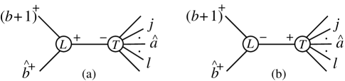
Figure 10: A non-standard factorization using an auxiliary ${[a,b\rangle}$ shift is assumed to be suppressed in the large-$z$ limit of the primary ${[j,l\rangle}$ shift, if the tree amplitude naively appearing in the factorization contains both legs $j$ and $l$ and is suppressed.

For multi-particle channels, factorization in complex momenta is the same as in real momenta. For two-particle channels with opposite-helicity gluons, the discussion in section III.2 showed that only the standard tree-level tensor structure contributes, and that for scalars in the loop the relevant form factor actually vanishes. For like-helicity gluons, in the complex kinematics for which the tree vertex is non-vanishing, the situation is more complicated. The structure of the factorization is known empirically for one of the two possible helicities of the intermediate gluon, for the case where the other possible intermediate helicity vanishes. This case occurs in studying the finite series of $n$-gluon amplitudes $A_{n}^{1\mbox{-}\rm loop}(1^{-},2^{+},\ldots,n^{+})$. The factorization has the form OnShellRecurrenceI ,

$$A_{n}^{1\mbox{-}\rm loop}(1,\ldots,b^{+},(b+1)^{+},\ldots,n)\rightarrow$$

$$\hskip 28.45274pt{i\over(s_{b(b+1)})^{2}}V_{3}^{1\mbox{-}\rm loop}(-K^{+},b^{+},(b+1)^{+})A_{n-1}^{\rm tree}(1,\ldots,K^{-},\ldots,n)$$ (99)

$$\hskip 56.9055pt\hbox{}\times(1\ +\ \mbox{\rm correction factors})\,.$$

This configuration is shown schematically in fig. 10(a). So long as the legs shifted under the original, primary, shift are both contained on the $A^{\rm tree}$ side of the factorization, the form of the correction factors in eq. (99) is such that the term vanishes as the primary shift variable $z\rightarrow\infty$, because the tree amplitude vanishes in that limit. We will defer a general study of the structure for the other intermediate helicity shown in fig. 10(b); the only property that we will need is the vanishing of the primary shift $z\rightarrow\infty$ limit for contributions where both shifted legs are on the tree side of the factorization, as in fig. 10. This property holds for previously-computed five- and six-point amplitudes GGGGG ; Bootstrap , and we will assume it holds more generally for both intermediate helicity configurations. The validity of this assumption can be tested at the end of a calculation, by checking all the symmetry and factorization properties of the fully assembled amplitude.

The auxiliary shift gives us the following expression for the complete amplitude,

$$A_{n}(0)=c_{\Gamma}\Bigl{[}{\widehat{C}}_{n}(0)-\mathop{\rm Inf}_{{[a,b\rangle}}{{\widehat{C}}_{n}}+R^{D,{[a,b\rangle}}_{n}+O_{n}^{{[a,b\rangle}}\Bigr{]}\,,$$ (100)

where the superscript ${[a,b\rangle}$ denotes the legs shifted under the auxiliary shift, and where the recursive diagrams are built and the overlap contributions determined, with respect to this shift. The large-parameter (large-$w$) terms of the auxiliary shift (98) are absent by design. We can now extract the large-parameter (large-$z$) behavior with respect to the primary ${[j,l\rangle}$ shift,

$$\mathop{\rm Inf}_{{[j,l\rangle}}{A_{n}}=c_{\Gamma}\mathop{\rm Inf}_{{[j,l\rangle}}{\Bigl{[}{\widehat{C}}_{n}(0)-\mathop{\rm Inf}_{{[a,b\rangle}}{{\widehat{C}}_{n}}+R^{D,{[a,b\rangle}}_{n}+O_{n}^{{[a,b\rangle}}\Bigr{]}}\,.$$ (101)

Following the discussion above, we arrange the shifts so only channels with standard factorizations will survive in the large-$z$ limit of the ${[j,l\rangle}$ shift. In extracting the large-$z$ behavior, we must in general keep all non-vanishing contributions to the amplitude, which may arise not only from the recursive diagrams with respect to the auxiliary shift, but also from completed-cut or overlap terms. In many practical cases, however, the only surviving contributions are from a limited set of recursive diagrams. Indeed, the typical surviving term will have the form,

$$\mathop{\rm Inf}_{{[j,l\rangle}}{R}(k_{P_{1}},\ldots,\hat{k}_{a},\ldots,k_{P_{-1}},-{\hat{P}}^{h})\times{i\over P^{2}}\times A^{\rm tree}(k_{{\overline{P}}_{1}},\ldots,\hat{k}_{b},\ldots,k_{{\overline{P}}_{-1}},{\hat{P}}^{-h})\,,$$ (102)

where legs $j$ and $l$ are both on the loop side.

In the next section, we shall present shift choices for general helicity configurations that implement the approach outlined in this section: a primary shift free of non-standard channels, but having non-trivial large shift-parameter behavior, and an auxiliary shift free of non-trivial large shift-parameter behavior, but containing non-standard channels that in turn vanish at large values of the primary parameter.

VI General Helicities

As an illustration of our strategy, in this section we now present specific shift choices for determining the rational-function parts of generic one-loop $n$-gluon amplitudes. As discussed in previous sections we must choose a primary shift so that non-standard complex singularities do not occur in the recursion. If there are contributions from large values of the shift parameter $z$, we determine these using an auxiliary shift and recursion relation.

VI.1 Empirical Structure of the Amplitudes

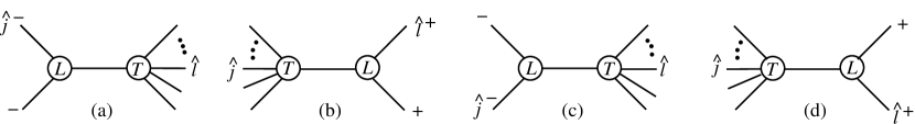
Figure 11: For a ${[j,l\rangle}$ shift, the four potential channels with non-standard complex singularities. Whether these are actually present in a given amplitude depends on the helicities of the legs nearest to $j$ and $l$ in the color ordering.

In order to proceed, we will need a few analytic properties of amplitudes. Unfortunately, as yet there are no theorems to guide us on the properties of complex factorizations of amplitudes or on the behavior of loop amplitudes under large complex shifts $z$. We therefore follow the empirical approach of refs. OnShellRecurrenceI ; Qpap ; Bootstrap . We observe certain useful properties of known amplitudes and then use these properties to aid in the computation of new amplitudes. We shall not prove these properties, noting that such proofs would be valuable to help guide future developments. This empirical approach has been effective for obtaining a variety of new one-loop amplitudes OnShellRecurrenceI ; Qpap ; Bootstrap ; FordeKosower . By now, a large number of QCD amplitudes are known analytically BKStringBased ; KunsztEtAl ; GGGGG ; QQQQG ; TwoQuarkThreeGluon ; AllPlus ; Mahlon ; OnShellRecurrenceI ; Qpap ; FordeKosower ; MHVQCDLoop , making it straightforward to develop a heuristic understanding of their analytic properties.

Our confidence in this pragmatic approach stems from the rather non-trivial checks that may be performed on any loop amplitude. In particular, the factorization properties of one-loop amplitudes in real momenta are well understood Neq4Oneloop ; Neq1Oneloop ; BernChalmers ; BDSSplit ; OneLoopSplitUnitarity and provide rather non-trivial constraints on the amplitudes by demanding that every pole in the amplitude corresponds to a physical factorization. The non-trivial consistency requirement stems from the fact that only a limited number of factorization channels enter into the recursive construction.

An investigation of the analytic properties of the known one-loop amplitudes reveals some striking properties:

1. For any ${[-,+\rangle}$ shift, all $n$-gluon amplitudes vanish for a large shift parameter, $z\rightarrow\infty$.

2. For $n$-gluon amplitudes with the split helicity configuration, $A_{n}(1^{-},2^{-},\ldots,(m-1)^{-},m^{+},(m+1)^{+},\ldots,n^{+})$, an alternative set of shifts where the amplitudes vanish at large $z$ are ${[1,m-1\rangle}$, ${[m-1,1\rangle}$, ${[m,n\rangle}$ and ${[n,m\rangle}$.

3. For a given ${[j,l\rangle}$ shift, there are no more than four channels with non-standard complex singularities, depending on the helicities of the legs nearest to $j$ and $l$, as depicted in fig. 11.

The above properties are by no means exhaustive. In particular, there are other shifts where one-loop $n$-gluon amplitudes vanish at large $z$, although the above observations will be sufficient for our purposes here.

As already discussed in section V.4, an empirical rule for suppressing diagrams with non-standard complex singularities in an auxiliary recursion relation is to ensure that the primary shift legs are both on the tree side of the naive factorization and that this tree amplitude is suppressed in the large-$z$ limit of the primary shift. Such configurations are displayed in fig. 10.

It is worth mentioning that based on our empirical studies of MHV supersymmetric amplitudes Neq4Oneloop ; Neq1Oneloop ; BST , it appears that in the supersymmetric case, the complete set of shifts where $A_{n}(z)$ vanishes for $z\rightarrow\infty$ is identical to the set of shifts where this is true at tree level, i.e. any ${[-,+\rangle},{[+,+\rangle}$ and ${[-,-\rangle}$ shift.

VI.2 Systematics for General Helicities

Using the above empirical observations, we now present a systematic procedure for finding pairs of shifts which will allow us to compute the rational terms in any $n$-gluon amplitude while avoiding non-standard complex singularities.

Depending on the helicity configuration, we will use the three independent shift choices:

• If the amplitude contains four color-neighboring legs having the helicity structure $i^{+},(i+1)^{-},(i+2)^{+},(i+3)^{-}$, then choose the shift ${[i+1,i+2\rangle}$. With this shift, the amplitude vanishes as $z\rightarrow\infty$ and no non-standard complex singularities appear in the recursion relation. Only a single shift, and hence only a single recursion relation, is required in this case.

• If the amplitude has three nearest neighboring legs $i^{-},(i+1)^{-},(i+2)^{+}$, choose ${[i+1,i\rangle}$ as the primary shift. For determining the behavior of the amplitudes for large values of the primary shift parameter, choose an auxiliary shift ${[a,b\rangle}$ such that $a$ is a negative-helicity leg, $b$ is a positive-helicity leg and $a\not=i-1,i,i+1$.

• For the special case of split helicity configurations, $A_{n}(1^{-},2^{-},\ldots,(m-1)^{-},m^{+},(m+1)^{+},\ldots,n^{+})$, a rather convenient choice is a primary ${[1,2\rangle}$ shift and an auxiliary ${[n,m\rangle}$ shift.

The above choices are not the complete set of choices that we need. However, all the remaining cases are simply related to the above ones via parity conjugation or a reversal of legs in the color ordering. For convenience, we also list these shift choices:

• If four neighboring legs in the color ordering have helicities $i^{-},(i+1)^{+},(i+2)^{-},(i+3)^{+}$ then choose the single shift ${[i+2,i+1\rangle}$.

• If the amplitude has three nearest-neighboring legs $i^{+},(i+1)^{-},(i+2)^{-}$, choose ${[i+1,i+2\rangle}$ as the primary shift. As the auxiliary shift choose any ${[a,b\rangle}$ such that $a$ is a negative-helicity leg, $b$ is a positive-helicity leg and $a\not=i+1,i+2,i+3$.

• If the amplitude has three nearest-neighboring legs $i^{-},(i+1)^{+},(i+2)^{+}$ choose ${[i+2,i+1\rangle}$ as the primary shift. As the auxiliary shift choose any ${[a,b\rangle}$ such that $a$ is a negative-helicity leg, $b$ is a positive-helicity leg and $b\not=i+1,i+2,i+3$.

Table 1: This table lists helicities and pairs of shifts that may be used to construct any six- or seven-gluon amplitude with three negative-helicity legs. The primary shift in the second column generates a recursion relation which does not have non-standard complex singularities, but the amplitude may not vanish for a large shift parameter $z$. Under the auxiliary shift in the third column, the recursion relation may have non-standard complex singularities in the channels listed in the fourth column. However, these singularities should be suppressed in the large-$z$ limit of the primary shift.

Helicity	Primary shift	Auxiliary shift	Suppressed channels
$1^{-},2^{-},3^{-},4^{+},5^{+}$	${[1,2\rangle}$	${[5,4\rangle}$	—
$1^{-},2^{-},3^{+},4^{-},5^{+}$	${[4,3\rangle}$	—	—
$1^{-},2^{-},3^{-},4^{+},5^{+},6^{+}$	${[1,2\rangle}$	${[6,4\rangle}$	$(45)$
$1^{-},2^{-},3^{+},4^{-},5^{+},6^{+}$	${[4,3\rangle}$	—	—
$1^{-},2^{+},3^{-},4^{+},5^{-},6^{+}$	${[1,2\rangle}$	—	—
$1^{-},2^{-},3^{-},4^{+},5^{+},6^{+},7^{+}$	${[1,2\rangle}$	${[7,4\rangle}$	$(45)$
$1^{-},2^{-},3^{+},4^{-},5^{+},6^{+},7^{+}$	${[4,3\rangle}$	—	—
$1^{-},2^{-},3^{+},4^{+},5^{-},6^{+},7^{+}$	${[1,2\rangle}$	${[5,6\rangle}$	$(67)$
$1^{-},2^{+},3^{-},4^{+},5^{-},6^{+},7^{+}$	${[3,4\rangle}$	—	—

With these choices we should then be able to construct the rational-function contributions of all unknown $n$-gluon amplitudes, once the cut-containing pieces are known. (The above choices are not useful for constructing amplitudes with identical helicities, but those are already known AllPlus ; Mahlon .) If more than one of the above choices is satisfied in a given amplitude, one may choose whichever is the most convenient. In Table 1 we have listed all the helicity configurations with three negative-helicity legs and up to seven external gluons, along with choices of primary and auxiliary shifts which may be used to construct the amplitudes. (In the first row, for $1^{-},2^{-},3^{-},4^{+},5^{+}$, our choice of auxiliary shift actually has no non-standard factorization channels, so it could be used by itself to fully determine the amplitude. We display this particular shift choice because it is based on the above rules and generalizes to the case of more adjacent positive-helicity gluons.)

It is important to note that there are many other valid shift pairs besides those in the above construction. For example, although we can use the rules to determine all amplitudes with two negative helicities, it turns out that a somewhat more convenient choice is to choose a ${[i,j\rangle}$ shift, where legs $i$ and $j$ are the two negative-helicity legs, as we shall discuss in a companion paper MHVQCDLoop . In many cases, it is also possible to relax the conditions we impose on the shifts. For example, we have been demanding that under the auxiliary shift the amplitude vanish for large shift parameter. In fact, this restriction is not necessary; we need only demand that any such terms do not contribute to the large shift terms of the primary shift. For example, the identical-helicity amplitudes $A_{n;1}(1^{+},2^{+},\ldots,n^{+})$ can be determined using a primary ${[5,7\rangle}$ shift and an auxiliary ${[1,3\rangle}$ shift (for $n\geq 7$), even though the amplitudes do not vanish OnShellRecurrenceI under the large-$z$ limit of either shift. In Table 2 we have collected a variety of examples of shift pairs which may be used to determine the amplitudes, but are outside the class of shifts described above for determining general helicity configurations.

Table 2: This table lists examples of valid shift pairs besides those selected by the procedure discussed in the text.

Helicity	Primary shift	Auxiliary shift	Suppressed channels
$1^{+},2^{+},\ldots,n^{+}$	${[5,7\rangle}$	${[1,3\rangle}$	—
$1^{-},2^{+},\ldots,j^{-},(j+1)^{+},\ldots,n^{+}$	${[1,j\rangle}$	—	—
$1^{-},2^{-},3^{-},4^{+},\ldots,n^{+}$	${[1,2\rangle}$	${[4,5\rangle}$	$(56)$
$1^{-},\ldots,(m-1)^{-},m^{+},\ldots,n^{+}$	${[1,2\rangle}$	${[m,m+1\rangle}$	$(m+1,m+2)$

We expect that a similar strategy will be effective for amplitudes with massless quarks, and for amplitudes with external massive vector bosons or Higgs particles. With suitable modifications it should be possible to use the on-shell bootstrap to construct amplitudes with massive particles in the loops as well.

VII Recursive Determinations of Large-$z$ Behavior

Following the procedure of the last section we now determine the large shift-parameter behavior of some sample amplitudes. We focus on amplitudes with three or four color-adjacent negative-helicity legs, as a non-trivial illustration of the method. Because the logarithmic terms in these amplitudes have already been calculated RecurCoeff , we can obtain the complete amplitudes by computing the rational terms recursively, as we do in the next section. We can confirm indirectly that our approach to determining the large-$z$ behavior is valid in these cases, by verifying that the amplitudes have the proper symmetries, and that they factorize correctly.

To determine the large-$z$ behavior of an amplitude, with the help of an auxiliary shift, one must include in general the large-$z$ behavior of the completed-cut, overlap and recursive contributions (with respect to the auxiliary shift). In subsection C, we shall encounter a five-point example where all three types of contributions are nonvanishing at large $z$. However, in subsections A and B, we shall arrange the shifts, for the respective cases of three and four color-adjacent negative helicities, so that the entire large-$z$ behavior comes from the recursive diagrams of the auxiliary shift. In this way it is very simple to obtain compact expressions for the large-$z$ behavior of these amplitudes under the ${[1,2\rangle}$ shift.

VII.1 $A_{n;1}^{{\cal N}=0}(1^{-},2^{-},3^{-},4^{+},5^{+},\ldots,n^{+})$

Consider now the $n$-gluon amplitudes with three color-adjacent negative-helicity legs. We use the special split-helicity shift choice described in the last section: a ${[1,2\rangle}$ shift as our primary shift, and an ${[n,4\rangle}$ shift as the auxiliary shift. This shift allows for an especially simple determination of the large-$z$ behavior in the $n$-point case.

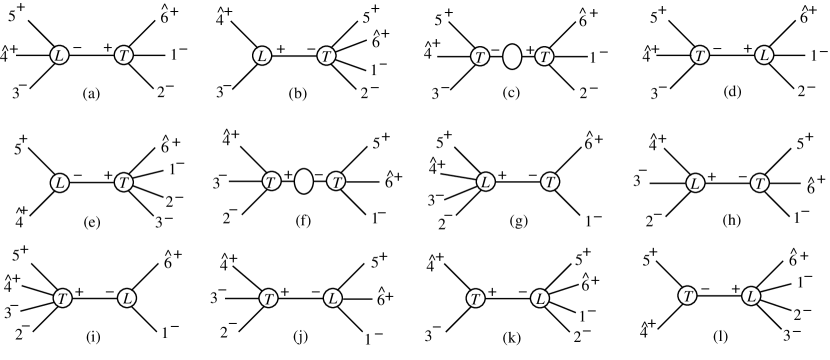
Figure 12: Recursive diagrams for $A_{6;1}^{{\cal N}=0}(1^{-},2^{-},3^{-},4^{+},5^{+},6^{+})$, for the auxiliary ${[6,4\rangle}$ shift. We drop the diagrams for which the tree vertex vanishes. Diagram (e) has non-standard complex singularities. Only diagrams (k) and (l) contribute to the large-$z$ limit of the ${[1,2\rangle}$ shift. Diagrams (c) and (f) represent the factorization-function contribution.

How do the individual contributions behave as the $z$ parameter associated with a ${[1,2\rangle}$ shift is taken to infinity? First consider the completed-cut contributions, ${\widehat{C}}_{n}$. These contributions were obtained in ref. RecurCoeff and are given in section VIII, eq. (124), where we describe them in more detail. As explained in that section, ${\widehat{C}}_{n}$ is non-vanishing in the large-$z$ limit of the ${[1,2\rangle}$ shift (see eq. (133)). However, a computation shows that the large-$z$ limit of the overlap terms obtained from ${\widehat{C}}_{n}$ cancels this term. So there are no large-$z$ ${[1,2\rangle}$ shift contributions arising from the sum of the completed-cut and overlap contributions of our auxiliary ${[n,4\rangle}$ shift. All that remains is to inspect the large-$z$ behavior of the recursive diagrams.

As a warm-up for the all-$n$ case, we consider the six-point case again, this time with an auxiliary ${[6,4\rangle}$ shift instead of ${[3,4\rangle}$. The recursive diagrams are shown in fig. 12, omitting diagrams where the tree vertex vanishes. The simplest diagrams to analyze are those where both shifted legs $1$ and $2$ are attached to a tree vertex in a ‘standard’ channel, as is true for figs. 12(a)–(c). The remainder of the diagram (the propagator and other vertex) is independent of the shift parameter, and so the large-parameter behavior is determined by the tree alone. Because this shift is a well-behaved shift at tree level BCFW ; GloverMassive , the tree vertex, and hence the diagram, vanishes in the large-$z$ limit. The same reasoning applies to diagrams where both shifted legs are attached to a loop vertex, and where we already know from previous computations that the ${[1,2\rangle}$ shift is well-behaved. This is the case for fig. 12(d). We cannot be certain that the same logic will apply to diagrams such as fig. 12(e), where both shifted legs are attached to a tree vertex, when the contribution is in a channel with non-standard factorization. Nonetheless, analysis of specific analogous cases leads us to conclude that these diagrams should be suppressed in the large-parameter limit. As discussed in the previous section, this assumption can be tested once the final answer for the amplitude is in hand. Diagrams where the shifted legs are attached to different vertices, such as those in figs. 12(f)–(j), must be analyzed explicitly. These diagrams involve only standard channels, and all do indeed vanish in the large-parameter limit.

This leaves us with two diagrams, those of figs. 12(k) and (l). Here, the shifted legs are both attached to the same five-point loop vertex with a standard factorization, so the large-parameter behavior is determined solely by the loop vertex. We know from eq. (29) that it has non-trivial behavior in that limit, which survives to contribute to the auxiliary recursion relation. Collecting these two contributions, we obtain the desired relation,

$$\mathop{\rm Inf}_{{[1,2\rangle}}{A^{{\cal N}=0}_{6;1}(1^{-},2^{-},3^{-},4^{+},5^{+},6^{+})}=$$

$$\hskip 56.9055pt\mathop{\rm Inf}_{{[1,2\rangle}}{A^{{\cal N}=0}_{5;1}(1^{-},2^{-},\hat{K}_{34}^{-},5^{+},\hat{6}^{+})}\,{i\over s_{34}}\,A_{3}^{\rm tree}(3^{-},\hat{4}^{+},-\hat{K}_{34}^{+})$$ (103)

$$\hskip 56.9055pt\hbox{}+\mathop{\rm Inf}_{{[1,2\rangle}}{A^{{\cal N}=0}_{5;1}(1^{-},2^{-},3^{-},\hat{K}_{45}^{+},\hat{6}^{+})}\,{i\over s_{45}}\,A_{3}^{\rm tree}(\hat{4}^{+},5^{+},-\hat{K}_{45}^{-})\,,$$

where $\hat{a}$ refers to legs shifted and frozen according to the auxiliary ${[6,4\rangle}$ shift. Evaluating this relation (and as we shall see below, even solving it for all $n$) is straightforward, thanks to its similarity to a tree-level MHV recursion relation BCFW . Plugging in the known values on the right-hand side, we obtain,

$$\mathop{\rm Inf}_{{[1,2\rangle}}{A}^{{\cal N}=0}_{6;1}(1^{-},2^{-},3^{-},4^{+},5^{+},6^{+}) = {ic_{\Gamma}\over 3}{\vphantom{\hat{K}}\left\langle\smash{1}\,\smash{\hat{K}_{34}}\right\rangle^{3}\left\langle 2\,\hat{6}\right\rangle\over\vphantom{\hat{K}}\left\langle\smash{1}\,\smash{\hat{6}}\right\rangle^{2}\vphantom{\hat{K}}\left\langle\smash{\hat{K}_{34}}\,\smash{5}\right\rangle\vphantom{\hat{K}}\left\langle\smash{5}\,\smash{\hat{6}}\right\rangle\left[1\,2\right]}\,{1\over s_{34}}\,{\vphantom{\hat{K}}\left[\smash{\hat{K}_{34}}\,\smash{\hat{4}}\right]^{3}\over\vphantom{\hat{K}}\left[\smash{3}\,\smash{\hat{4}}\right]\vphantom{\hat{K}}\left[\smash{\hat{K}_{34}}\,\smash{3}\right]}$$ (104)

$$\hbox{}+{ic_{\Gamma}\over 3}\,{\left\langle 1\,3\right\rangle^{3}\vphantom{\hat{K}}\left\langle\smash{2}\,\smash{\hat{6}}\right\rangle\over\vphantom{\hat{K}}\left\langle\smash{1}\,\smash{\hat{6}}\right\rangle^{2}\vphantom{\hat{K}}\left\langle\smash{3}\,\smash{\hat{K}_{45}}\right\rangle\vphantom{\hat{K}}\left\langle\smash{\hat{K}_{45}}\,\smash{\hat{6}}\right\rangle\left[1\,2\right]}\,{1\over s_{45}}\,{\vphantom{\hat{K}}\left[\smash{5}\,\smash{\hat{4}}\right]^{3}\over\vphantom{\hat{K}}\left[\smash{\hat{K}_{45}}\,\smash{5}\right]\vphantom{\hat{K}}\left[\smash{\hat{4}}\,\smash{\hat{K}_{45}}\right]}$$

$$= {ic_{\Gamma}\over 3}{\left\langle 1\,3\right\rangle^{3}\left\langle 2\,6\right\rangle\over\left\langle 1\,6\right\rangle^{2}\left\langle 3\,4\right\rangle\left\langle 4\,5\right\rangle\left\langle 5\,6\right\rangle\left[1\,2\right]}\,,$$

in agreement with eq. (44).

It is straightforward to generalize eq. (103) to obtain the large-$z$ behavior of the $n$-gluon amplitude under a ${[1,2\rangle}$ shift. Following the same logic, we obtain the recursion relation, using an auxiliary ${[n,4\rangle}$ shift,

$$\mathop{\rm Inf}_{{[1,2\rangle}}{A^{{\cal N}=0}_{n;1}(1^{-},2^{-},3^{-},4^{+},5^{+},\ldots,n^{+})}=$$

$$\hskip 56.9055pt\mathop{\rm Inf}_{{[1,2\rangle}}{A^{{\cal N}=0}_{n-1;1}(1^{-},2^{-},\hat{K}_{34}^{-},5^{+},\ldots,\hat{n}^{+})}\,{i\over s_{34}}\,A_{3}^{\rm tree}(3^{-},\hat{4}^{+},-\hat{K}_{34}^{+})$$ (105)

$$\hskip 56.9055pt\hbox{}+\mathop{\rm Inf}_{{[1,2\rangle}}{A^{{\cal N}=0}_{n-1;1}(1^{-},2^{-},3^{-},\hat{K}_{45}^{+},6^{+},\ldots,\hat{n}^{+})}\,{i\over s_{45}}\,A_{3}^{\rm tree}(\hat{4}^{+},5^{+},-\hat{K}_{45}^{-})\,,$$

where we assumed that diagrams involving non-standard factorization, and diagrams where legs 1 and 2 appear on different vertices, are suppressed at large $z$, the same way they were at six points. Solving this recursion relation by induction, we obtain the large $z$ behavior at $n$ points,

$$\mathop{\rm Inf}_{{[1,2\rangle}}{A^{{\cal N}=0}_{n;1}(1^{-},2^{-},3^{-},4^{+},\ldots,n^{+})}={ic_{\Gamma}\over 3}{\left\langle 1\,3\right\rangle^{3}\left\langle 2\,n\right\rangle\over\left[1\,2\right]\left\langle n\,1\right\rangle^{2}\prod\limits_{k=3}^{n-1}\left\langle k\,(k+1)\right\rangle}\,.$$ (106)

We will use this result in the next section to construct a recursive solution for the rational functions in the $n$-point amplitude.

VII.2 $A_{n;1}^{{\cal N}=0}(1^{-},2^{-},3^{-},4^{-},5^{+},\ldots,n^{+})$.

We now consider the case of four color-adjacent negative helicities. Once again it is useful to illustrate the six-point case, $A_{6;1}^{{\cal N}=0}(1^{-},2^{-},3^{-},4^{-},5^{+},6^{+})$, before turning to the $n$-point case. Following the discussion of the previous section, a convenient pair of shifts is the ${[1,2\rangle}$ shift as the primary shift and the ${[4,5\rangle}$ shift as the auxiliary shift for determining the large-$z$ behavior of the amplitude under the primary shift. (An alternative choice would be an auxiliary ${[n,5\rangle}$ shift.)

As was the case for three color-adjacent negative helicities, an examination of the cut terms given in ref. RecurCoeff reveals that in the large-$z$ limit of the ${[1,2\rangle}$ shift there are no contributions from the sum of the completed-cut and overlap contributions. So here we focus on the non-vanishing rational-recursive contributions.

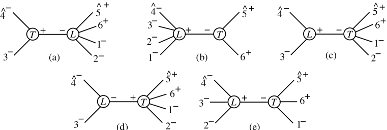
Figure 13: Non-vanishing recursive diagrams for $A_{6;1}^{{\cal N}=0}(1^{-},2^{-},3^{-},4^{-},5^{+},6^{+})$, for the auxiliary ${[4,5\rangle}$ shift. We use this recursion to determine the large-$z$ behavior under the primary ${[1,2\rangle}$ shift. Only diagrams (a) and (b) contribute to the large-$z$ limit.

The auxiliary ${[4,5\rangle}$ shift diagrams are shown in fig. 13 and are given by

$$R^{D,{[4,5\rangle}}_{6}(1^{-},2^{-},3^{-},4^{-},5^{+},6^{+}) = D^{\rm(a)}+D^{\rm(b)}+D^{\rm(c)}+D^{\rm(d)}+D^{\rm(e)}$$ (107)

$$= A_{3}^{\rm tree}(3^{-},\hat{4}^{-},-\hat{K}_{34}^{+}){i\over s_{34}}R_{5}(1^{-},2^{-},\hat{K}_{34}^{-},\hat{5}^{+},6^{+})$$

$$\hbox{}+R_{5}(1^{-},2^{-},3^{-},\hat{4}^{-},\hat{K}_{56}^{+}){i\over s_{56}}A_{3}^{\rm tree}(\hat{5}^{+},6^{+},-\hat{K}_{56}^{-})$$

$$\hbox{}+R_{3}(3^{-},\hat{4}^{-},-\hat{K}_{34}^{+}){i\over s_{34}}A_{5}^{\rm tree}(1^{-},2^{-},\hat{K}_{34}^{-},\hat{5}^{+},6^{+})$$

$$\hbox{}+R_{3}(3^{-},\hat{4}^{-},-\hat{K}_{34}^{-}){i\over s_{34}}A_{5}^{\rm tree}(1^{-},2^{-},\hat{K}_{34}^{+},\hat{5}^{+},6^{+})$$

$$\hbox{}+R_{4}(2^{-},3^{-},\hat{4}^{-},-\hat{K}_{234}^{+}){i\over s_{234}}A_{4}^{\rm tree}(1^{-},\hat{K}_{234}^{-},\hat{5}^{+},6^{+})\,,\hskip 28.45274pt$$

where $\hat{a}$ denotes momenta shifted and frozen according to the auxiliary ${[4,5\rangle}$ shift. We apply the ${[1,2\rangle}$ shift to this recursion relation and then take the large-$z$ limit of this primary shift. We assume that diagrams (c) and (d), which contain non-standard complex singularities, are suppressed in this limit (as discussed in section V.4), because the corresponding tree vertices are suppressed.

Diagram (e) is also suppressed, but that requires a closer inspection. To analyze diagram (e) we need the vertex, obtained by parity conjugation from eq. (168),

$$R_{4}(1^{+},2^{-},3^{-},4^{-})={i\over 3}{\left[2\,4\right]\left\langle 2\,4\right\rangle^{3}\over\left\langle 1\,2\right\rangle\left[2\,3\right]\left[3\,4\right]\left\langle 4\,1\right\rangle}\,.$$ (108)

Then diagram (e) is,

$$D^{\rm(e)} = R_{4}(2^{-},3^{-},\hat{4}^{-},-\hat{K}_{234}^{+}){i\over s_{234}}A_{4}^{\rm tree}(1^{-},\hat{K}_{234}^{-},\hat{5}^{+},6^{+})$$ (109)

$$= {i\over 3}{\vphantom{\hat{K}}\left[\smash{2}\,\smash{\hat{4}}\right]\left\langle 2\,\hat{4}\right\rangle^{3}\over\vphantom{\hat{K}}\left\langle\smash{\hat{K}_{234}}\,\smash{2}\right\rangle\left[2\,3\right]\vphantom{\hat{K}}\left[\smash{3}\,\smash{\hat{4}}\right]\vphantom{\hat{K}}\left\langle\smash{\hat{4}}\,\smash{\hat{K}_{234}}\right\rangle}{1\over s_{234}}{\vphantom{\hat{K}}\left\langle\smash{1}\,\smash{\hat{K}_{234}}\right\rangle^{3}\over\vphantom{\hat{K}}\left\langle\smash{\hat{K}_{234}}\,\smash{\hat{5}}\right\rangle\vphantom{\hat{K}}\left\langle\smash{\hat{5}}\,\smash{6}\right\rangle\left\langle 6\,1\right\rangle}$$

$$= {i\over 3}{\vphantom{\hat{K}}\left[\smash{2}\,\smash{\hat{4}}\right]\left\langle 2\,4\right\rangle^{3}\over\left\langle\smash{2}{\vphantom{1}}^{-}\right|{{\raise 0.91666pt\hbox to9.20833pt{\hss/\hss}\hbox to0.0pt{\hss$K$}}_{234}}\left|\smash{5}{\vphantom{1}}^{-}\right\rangle\left[2\,3\right]\vphantom{\hat{K}}\left[\smash{3}\,\smash{\hat{4}}\right]\left\langle\smash{4}{\vphantom{1}}^{-}\right|{{\raise 0.91666pt\hbox to9.20833pt{\hss/\hss}\hbox to0.0pt{\hss$K$}}_{234}}\left|\smash{5}{\vphantom{1}}^{-}\right\rangle}{1\over s_{234}}{\left\langle\smash{1}{\vphantom{1}}^{-}\right|{{\raise 0.91666pt\hbox to9.20833pt{\hss/\hss}\hbox to0.0pt{\hss$K$}}_{234}}\left|\smash{5}{\vphantom{1}}^{-}\right\rangle^{3}\over\left\langle\smash{\hat{5}}{\vphantom{1}}^{-}\right|{{\raise 0.91666pt\hbox to9.20833pt{\hss/\hss}\hbox to0.0pt{\hss$K$}}_{234}}\left|\smash{5}{\vphantom{1}}^{-}\right\rangle\vphantom{\hat{K}}\left\langle\smash{\hat{5}}\,\smash{6}\right\rangle\left\langle 6\,1\right\rangle}\,.\hskip 28.45274pt$$

We can simplify this term further, by substituting in the remaining hatted variables, which become independent of $z$ as $z\to\infty$; but already in this form we can see that it vanishes in the large-$z$ limit of the ${[1,2\rangle}$ shift. Therefore diagram (e) does not contribute to the recursion relation for the large-$z$ terms.

Thus we obtain a very simple recursion relation for the non-vanishing large-$z$ terms, based only on diagrams (a) and (b),

$$\mathop{\rm Inf}_{{[1,2\rangle}}{A^{{\cal N}=0}_{6;1}(1^{-},2^{-},3^{-},4^{-},5^{+},6^{+})} = A_{3}^{\rm tree}(3^{-},\hat{4}^{-},-\hat{K}_{34}^{+})\,{i\over s_{34}}\,\mathop{\rm Inf}_{{[1,2\rangle}}{A^{{\cal N}=0}_{5;1}(1^{-},2^{-},\hat{K}_{34}^{-},\hat{5}^{+},6^{+})}$$

$$\hbox{}+A_{3}^{\rm tree}(\hat{5}^{+},6^{+},-\hat{K}_{56}^{-})\,{i\over s_{56}}\,\mathop{\rm Inf}_{{[1,2\rangle}}{A^{{\cal N}=0}_{5;1}(1^{-},2^{-},3^{-},\hat{4}^{-},\hat{K}_{56}^{+})}\,.$$

On the right-hand side there are two large-$z$ contributions. The first one is familiar from eq. (39),

$$\mathop{\rm Inf}_{{[1,2\rangle}}{A^{{\cal N}=0}_{5;1}(1^{-},2^{-},3^{-},4^{+},5^{+})}=i\,{c_{\Gamma}\over 3}{\left\langle 1\,3\right\rangle^{3}\left\langle 2\,5\right\rangle\over\left[1\,2\right]\left\langle 5\,1\right\rangle^{2}\left\langle 3\,4\right\rangle\left\langle 4\,5\right\rangle}\,.$$ (111)

To get the second one, we start from formula (LABEL:A5Neq0mpppp) for $A^{{\cal N}=0}_{5;1}(1^{-},2^{+},3^{+},4^{+},5^{+})$, relabel, and take the parity conjugate, to get,

$$A^{{\cal N}=0}_{5;1}(1^{-},2^{-},3^{-},4^{-},5^{+})=-i\,{c_{\Gamma}\over 3}\,{1\over\left[2\,3\right]^{2}}\Biggl{[}-{\left\langle 1\,4\right\rangle^{3}\over\left\langle 5\,1\right\rangle\left\langle 4\,5\right\rangle}+{\left[5\,3\right]^{3}\left\langle 3\,4\right\rangle\left[2\,4\right]\over\left[5\,1\right]\left[1\,2\right]\left[3\,4\right]^{2}}-{\left[5\,2\right]^{3}\left\langle 2\,1\right\rangle\left[3\,1\right]\over\left[5\,4\right]\left[4\,3\right]\left[2\,1\right]^{2}}\Biggr{]}\,.$$ (112)

Applying the ${[1,2\rangle}$ shift and extracting the $z^{0}$ terms gives us the desired contribution, which we wish to feed into the recursion,

$$\mathop{\rm Inf}_{{[1,2\rangle}}{A^{{\cal N}=0}_{5;1}(1^{-},2^{-},3^{-},4^{-},5^{+})}=-i\,{c_{\Gamma}\over 3}\,{1\over\left[2\,3\right]^{2}}\Biggl{[}-{\left\langle 1\,4\right\rangle^{3}\over\left\langle 5\,1\right\rangle\left\langle 4\,5\right\rangle}-{\left[5\,2\right]^{3}\left\langle 2\,1\right\rangle\left[3\,1\right]\over\left[5\,4\right]\left[4\,3\right]\left[2\,1\right]^{2}}\Biggr{]}\,.$$ (113)

Relabeling and inserting the large-$z$ terms (111) and (113) into the recursion (LABEL:Boundary12Recursion45) we obtain,

$$\mathop{\rm Inf}_{{[1,2\rangle}}{A^{{\cal N}=0}_{6;1}(1^{-},2^{-},3^{-},4^{-},5^{+},6^{+})}$$

$$\hbox{}\hskip 48.36958pt=A_{3}^{\rm tree}(3^{-},\hat{4}^{-},-\hat{K}_{34}^{+})\,{i\over s_{34}}\,\mathop{\rm Inf}_{{[1,2\rangle}}{A^{{\cal N}=0}_{5;1}(1^{-},2^{-},\hat{K}_{34}^{-},\hat{5}^{+},6^{+})}$$

$$\hskip 62.59596pt\hbox{}+A_{3}^{\rm tree}(\hat{5}^{+},6^{+},-\hat{K}_{56}^{-})\,{i\over s_{56}}\,\mathop{\rm Inf}_{{[1,2\rangle}}{A^{{\cal N}=0}_{5;1}(1^{-},2^{-},3^{-},\hat{4}^{-},\hat{K}_{56}^{+})}$$

$$\hbox{}\hskip 48.36958pt=i\,{c_{\Gamma}\over 3}{\vphantom{\hat{K}}\left\langle\smash{3}\,\smash{\hat{4}}\right\rangle^{3}\over\vphantom{\hat{K}}\left\langle\smash{\hat{4}}\,\smash{\hat{K}_{34}}\right\rangle\vphantom{\hat{K}}\left\langle\smash{\hat{K}_{34}}\,\smash{3}\right\rangle}\,{1\over s_{34}}\,{\vphantom{\hat{K}}\left\langle\smash{1}\,\smash{\hat{K}_{34}}\right\rangle^{3}\left\langle 2\,6\right\rangle\over\left[1\,2\right]\left\langle 6\,1\right\rangle^{2}\vphantom{\hat{K}}\left\langle\smash{\hat{K}_{34}}\,\smash{\hat{5}}\right\rangle\left\langle\hat{5}\,6\right\rangle}$$

$$\hskip 62.59596pt\hbox{}+i\,{c_{\Gamma}\over 3}{\vphantom{\hat{K}}\left[\smash{\hat{5}}\,\smash{6}\right]^{3}\over\vphantom{\hat{K}}\left[\smash{\hat{5}}\,\smash{\hat{K}_{56}}\right]\vphantom{\hat{K}}\left[\smash{\hat{K}_{56}}\,\smash{6}\right]}\,{1\over s_{56}}\,{1\over\left[2\,3\right]^{2}}\Biggl{[}-{\left\langle 1\,\hat{4}\right\rangle^{3}\over\vphantom{\hat{K}}\left\langle\smash{\hat{K}_{56}}\,\smash{1}\right\rangle\vphantom{\hat{K}}\left\langle\smash{\hat{4}}\,\smash{\hat{K}_{56}}\right\rangle}-{\vphantom{\hat{K}}\left[\smash{\hat{K}_{56}}\,\smash{2}\right]^{3}\left\langle 2\,1\right\rangle\left[3\,1\right]\over\vphantom{\hat{K}}\left[\smash{\hat{K}_{56}}\,\smash{\hat{4}}\right]\vphantom{\hat{K}}\left[\smash{\hat{4}}\,\smash{3}\right]\left[2\,1\right]^{2}}\Biggr{]}$$

$$\hbox{}\hskip 48.36958pt=i\,{c_{\Gamma}\over 3}\Biggl{[}{\left\langle\smash{1}{\vphantom{1}}^{-}\right|{(3+4)}\left|\smash{5}{\vphantom{1}}^{-}\right\rangle^{3}\left\langle 2\,6\right\rangle\over\left[1\,2\right]\left[3\,4\right]\left[4\,5\right]\left\langle 6\,1\right\rangle^{2}s_{345}\left\langle\smash{6}{\vphantom{1}}^{-}\right|{(4+5)}\left|\smash{3}{\vphantom{1}}^{-}\right\rangle}$$ (114)

$$\hbox{}\hskip 85.35826pt+{\left\langle 1\,4\right\rangle^{3}\over\left[2\,3\right]^{2}\left\langle 4\,5\right\rangle\left\langle 5\,6\right\rangle\left\langle 6\,1\right\rangle}+{\left\langle\smash{4}{\vphantom{1}}^{-}\right|{(5+6)}\left|\smash{2}{\vphantom{1}}^{-}\right\rangle^{3}\left\langle 2\,1\right\rangle\left[1\,3\right]\over\left[1\,2\right]^{2}\left[2\,3\right]^{2}\left\langle 4\,5\right\rangle\left\langle 5\,6\right\rangle s_{456}\left\langle\smash{6}{\vphantom{1}}^{-}\right|{(4+5)}\left|\smash{3}{\vphantom{1}}^{-}\right\rangle}\Biggr{]}\,.$$

We have checked that this result is in agreement with the large-$z$ behavior extracted from the parity conjugation of the six-point amplitude obtained in ref. Bootstrap .

It is straightforward to generalize the discussion to $n$-point amplitudes. Following the same logic as for six points, we obtain a recursion relation for the large-$z$ behavior under the ${[1,2\rangle}$ shift,

$$\mathop{\rm Inf}_{{[1,2\rangle}}{A^{{\cal N}=0}_{n;1}(1^{-},2^{-},3^{-},4^{-},5^{+},\ldots,n^{+})}$$ (115)

$$\hskip 56.9055pt\hbox{}=A_{3}^{\rm tree}(3^{-},\hat{4}^{-},-\hat{K}_{34}^{+}){i\over s_{34}}\mathop{\rm Inf}_{{[1,2\rangle}}{A^{{\cal N}=0}_{n-1;1}(1^{-},2^{-},\hat{K}_{34}^{-},\hat{5}^{+},\ldots,n^{+})}$$

$$\hskip 68.28644pt\hbox{}+A_{3}^{\rm tree}(\hat{5}^{+},6^{+},-\hat{K}_{56}^{-})\,{i\over s_{56}}\,\mathop{\rm Inf}_{{[1,2\rangle}}{A^{{\cal N}=0}_{n-1;1}(1^{-},2^{-},3^{-},\hat{4}^{-},\hat{K}_{56}^{+},7^{+},\ldots,n^{+})}\,.$$

We have solved this recursion relation with the result,

$$\hskip-8.5359pt\mathop{\rm Inf}_{{[1,2\rangle}}{A^{{\cal N}=0}_{n;1}(1^{-},2^{-},3^{-},4^{-},5^{+},\ldots,n^{+})}$$ (116)

$$\hskip 17.07182pt\hbox{}=i\,{c_{\Gamma}\over 3}\Biggl{[}{\left\langle 1\,4\right\rangle^{3}\over\left[2\,3\right]^{2}\prod\limits_{k=4}^{n-1}\left\langle k\,(k+1)\right\rangle\left\langle n\,1\right\rangle}+{\left\langle\smash{4}{\vphantom{1}}^{-}\right|{{\raise 0.91666pt\hbox to9.20833pt{\hss/\hss}\hbox to0.0pt{\hss$K$}}_{5\ldots n}}\left|\smash{2}{\vphantom{1}}^{-}\right\rangle^{3}\left\langle 2\,1\right\rangle\left[1\,3\right]\over s_{4\ldots n}\left\langle\smash{n}{\vphantom{1}}^{-}\right|{{\raise 0.91666pt\hbox to9.20833pt{\hss/\hss}\hbox to0.0pt{\hss$K$}}_{4\ldots n}}\left|\smash{3}{\vphantom{1}}^{-}\right\rangle\left[1\,2\right]^{2}\left[2\,3\right]^{2}\prod\limits_{k=4}^{n-1}\left\langle k\,(k+1)\right\rangle}$$

$$\hskip 51.21504pt\hbox{}+\sum_{j=5}^{n-1}{\left\langle j\,(j+1)\right\rangle\left\langle\smash{1}{\vphantom{1}}^{-}\right|{{\raise 0.91666pt\hbox to9.20833pt{\hss/\hss}\hbox to0.0pt{\hss$K$}}_{3\ldots j}{\raise 0.91666pt\hbox to9.20833pt{\hss/\hss}\hbox to0.0pt{\hss$K$}}_{5\ldots j}}\left|\smash{4}{\vphantom{1}}^{+}\right\rangle^{3}\left\langle 2\,n\right\rangle\over s_{3\ldots j}s_{4\ldots j}\left\langle\smash{(j+1)}{\vphantom{1}}^{-}\right|{{\raise 0.91666pt\hbox to9.20833pt{\hss/\hss}\hbox to0.0pt{\hss$K$}}_{4\ldots j}}\left|\smash{3}{\vphantom{1}}^{-}\right\rangle\left\langle\smash{j}{\vphantom{1}}^{-}\right|{{\raise 0.91666pt\hbox to9.20833pt{\hss/\hss}\hbox to0.0pt{\hss$K$}}_{4\ldots j}}\left|\smash{3}{\vphantom{1}}^{-}\right\rangle\left[1\,2\right]\prod\limits_{k=4}^{n-1}\left\langle k\,(k+1)\right\rangle\left\langle n\,1\right\rangle^{2}}\Biggr{]}\,.$$

VII.3 Another Look at $A_{5;1}^{{\cal N}=0}(1^{-},2^{-},3^{-},4^{+},5^{+})$

In the two previous subsections, the completed-cut and overlap contributions did not contribute to the large-$z$ terms of the primary shift. However, as we now illustrate, this is not always true. We reexamine the large-$z$ limit of the five-point amplitude $A_{5;1}^{{\cal N}=0}(1^{-},2^{-},3^{-},4^{+},5^{+})$ under a ${[1,2\rangle}$ shift. This example was already considered in section III. However, here we recursively construct the large-$z$ behavior by using a different auxiliary shift, a ${[4,5\rangle}$ shift. Although there are no non-standard factorization channels here, the example displays several important features: The large-$z$ recursive contribution comes entirely from a diagram where legs 1 and 2, the primary shift legs, are split across the pole of the auxiliary shift. Also, as was just mentioned, we need to account for contributions from completed-cut and overlap terms under the auxiliary shift.

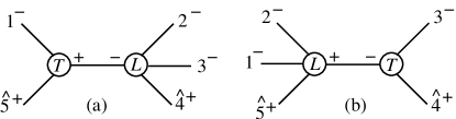
Figure 14: Nonvanishing diagrams of the ${[4,5\rangle}$ shift recursion relation for $A_{5;1}^{{\cal N}=0}(1^{-},2^{-},3^{-},4^{+},5^{+})$. Only diagram (a), which has legs 1 and 2 on opposite sides of the pole, contributes to the large-$z$ limit of the ${[1,2\rangle}$ shift.

The nonvanishing recursive diagrams of the auxiliary ${[4,5\rangle}$ shift are shown in fig. 14. First observe that the behavior of diagram (b) under the ${[1,2\rangle}$ shift is determined by the rational part of the four-point one-loop MHV amplitude with adjacent negative helicities, which is proportional to the tree amplitude, according to eq. (175). Tree amplitudes vanish at large $z$ for shifts of identical-helicity pairs of legs BCFW ; GloverMassive ; hence diagram (b) does not contribute to the large-$z$ limit. Therefore, we need only evaluate the contribution of diagram (a). Here we find a new feature: The shifted legs of the primary ${[1,2\rangle}$ shift cross the pole in the auxiliary recursion relation. Nevertheless, the large-$z$ contribution can be determined just as in the previous examples. This pole-crossing contribution is given by,

$${R^{D,\rm(a)}_{5}} = A_{3}^{{\rm tree}}(1^{-},-\hat{K}_{51}^{+},\hat{5}^{+}){i\over s_{51}}R_{4}(2^{-},3^{-},\hat{4}^{+},\hat{K}_{51}^{-})$$ (117)

$$= {i\over 3}{\vphantom{\hat{K}}\left[\smash{\hat{K}_{51}}\,\smash{3}\right]{\vphantom{\hat{K}}\left\langle\smash{\hat{K}_{51}}\,\smash{3}\right\rangle}^{3}\over\left[2\,3\right]\vphantom{\hat{K}}\left\langle\smash{3}\,\smash{\hat{4}}\right\rangle\vphantom{\hat{K}}\left\langle\smash{\hat{4}}\,\smash{\hat{K}_{51}}\right\rangle\vphantom{\hat{K}}\left[\smash{\hat{K}_{51}}\,\smash{2}\right]}{1\over s_{51}}{{\vphantom{\hat{K}}\left[\smash{\hat{5}}\,\smash{\hat{K}_{51}}\right]}^{3}\over{\vphantom{\hat{K}}\left[\smash{1}\,\smash{\hat{K}_{51}}\right]}\vphantom{\hat{K}}\left[\smash{\hat{5}}\,\smash{1}\right]}\,,$$

where $\hat{a}$ refers to legs shifted according to the auxiliary ${[4,5\rangle}$ shift. We then obtain in the large-$z$ limit of the ${[1,2\rangle}$ shift the contribution,

$$\mathop{\rm Inf}_{{[1,2\rangle}}{R^{D,{[4,5\rangle}}_{5}(1^{-},2^{-},3^{-},4^{+},5^{+})}=-{i\over 3}{{\left\langle 1\,3\right\rangle}^{3}{\left\langle 2\,4\right\rangle}\over\left[2\,3\right]{\left\langle 3\,4\right\rangle}^{2}\left\langle 4\,5\right\rangle\left\langle 5\,1\right\rangle}\,.$$ (118)

Comparing eq. (118) to the known expression in eq. (39) we see that the two expressions do not match. However, we also have to take into account the contributions to the large-$z$ limit from the overlap contributions as indicated in eq. (95). We apply the ${[4,5\rangle}$ shift to ${\widehat{CR}}_{5}$, which can be extracted from eq. (31). We obtain the overlap contribution from the residues of ${\widehat{CR}}_{5}(w)/w$ at the following values of $w$, illustrated in fig. 15,

$$w^{\rm(a)}=-{\left\langle 1\,5\right\rangle\over\left\langle 1\,4\right\rangle}\,,\hskip 71.13188ptw^{\rm(b)}={\left[3\,4\right]\over\left[3\,5\right]}\,.$$ (119)

Evaluating these in the standard way, we obtain the large-$z$ contributions,

$$\mathop{\rm Inf}_{{[1,2\rangle}}{O_{5}^{\rm(a),\,{[4,5\rangle}}} = -{i\over 3}{{\left\langle 1\,3\right\rangle}^{2}\left[2\,5\right]\left\langle 2\,3\right\rangle\over\left[1\,2\right]\left[2\,3\right]{\left\langle 3\,4\right\rangle}^{2}\left\langle 5\,1\right\rangle}-{i\over 6}{{\left\langle 1\,3\right\rangle}^{2}\left[4\,5\right]\over\left[1\,2\right]\left[2\,3\right]{\left\langle 3\,4\right\rangle}\left\langle 5\,1\right\rangle}\,,$$ (120)

$$\mathop{\rm Inf}_{{[1,2\rangle}}{O_{5}^{\rm(b),\,{[4,5\rangle}}} = {i\over 6}{\left\langle 1\,3\right\rangle{\left[4\,5\right]}^{2}\over{\left[1\,2\right]}\left[2\,3\right]s_{34}}\,.$$ (121)

Notice that both eqs. (118) and (120) have double poles in $1/\left\langle 3\,4\right\rangle$, which cancel correctly upon adding up all contributions.

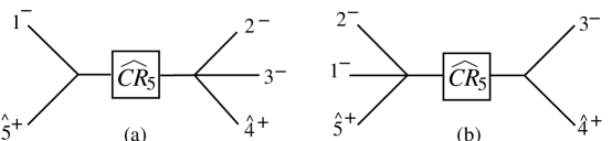
Figure 15: The overlap diagrams of the ${[4,5\rangle}$ shift.

Finally, we need to take into account the contribution from the completed-cut terms ${\widehat{C}}_{5}$, which are easily found to be,

$$\mathop{\rm Inf}_{{[1,2\rangle}}{{\widehat{C}}_{5}(1^{-},2^{-},3^{-},4^{+},5^{+})}=-{i\over 6}{{\left\langle 1\,2\right\rangle}\left[2\,4\right]\left\langle 1\,3\right\rangle\left(\left\langle 1\,2\right\rangle\left[2\,4\right]-\left\langle 1\,3\right\rangle\left[3\,4\right]\right)\over\left[1\,2\right]\left[2\,3\right]{\left\langle 5\,1\right\rangle}^{2}s_{34}}\,.$$ (122)

Upon adding all contributions, eqs. (118), (120), (121), and (122), we obtain

$$\mathop{\rm Inf}_{{[1,2\rangle}}{A_{5;1}^{{\cal N}=0}} = -i\,{c_{\Gamma}}\,\Biggl{[}{1\over 3}{{\left\langle 1\,3\right\rangle}^{3}\left\langle 2\,4\right\rangle\over\left[2\,3\right]\left\langle 3\,4\right\rangle^{2}\left\langle 4\,5\right\rangle\left\langle 5\,1\right\rangle}+\,{1\over 3}{{\left\langle 1\,3\right\rangle}^{2}\left[2\,5\right]\left\langle 2\,3\right\rangle\over\left[1\,2\right]\left[2\,3\right]{\left\langle 3\,4\right\rangle}^{2}\left\langle 5\,1\right\rangle}+{1\over 6}{{\left\langle 1\,3\right\rangle}^{2}\left[4\,5\right]\over\left[1\,2\right]\left[2\,3\right]{\left\langle 3\,4\right\rangle}\left\langle 5\,1\right\rangle}$$ (123)

$$\hskip 34.14322pt-{1\over 6}{\left\langle 1\,3\right\rangle{\left[4\,5\right]}^{2}\over{\left[1\,2\right]}\left[2\,3\right]s_{34}}+{1\over 6}{{\left\langle 1\,2\right\rangle}\left[2\,4\right]\left\langle 1\,3\right\rangle\left(\left\langle 1\,2\right\rangle\left[2\,4\right]-\left\langle 1\,3\right\rangle\left[3\,4\right]\right)\over\left[1\,2\right]\left[2\,3\right]{\left\langle 5\,1\right\rangle}^{2}s_{34}}\Biggr{]}$$

$$= i\,{c_{\Gamma}\over 3}{\left\langle 1\,3\right\rangle^{3}\left\langle 2\,5\right\rangle\over\left\langle 1\,5\right\rangle^{2}\left\langle 3\,4\right\rangle\left\langle 4\,5\right\rangle\left[1\,2\right]}\,,$$

in agreement with eq. (39).

This example demonstrates that, in general, if we wish to obtain the correct large-$z$ behavior using an auxiliary recursion, we must include the contributions from the completed-cut and overlap terms. In practice, however, often only the recursive diagrams contribute.

VIII Complete Split Helicity Amplitudes

In section VII.1 we determined the large-$z$ behavior, under a ${[1,2\rangle}$ shift, of the $n$-point amplitudes with three nearest-neighboring negative helicities, $A_{n;1}^{{\cal N}=0}(1^{-},2^{-},3^{-},4^{+},\ldots,n^{+})$. We now use this result to evaluate the remaining rational terms, using the formalism described in section V. The $n$-point tree amplitudes for these helicity configurations were determined in refs. DAKRecurrence ; CSW ; TreeRecurResults ; RoibanSplitHelicity , and are given in eq. (A).

VIII.1 Cut Contributions

The completed-cut contributions for general split-helicity ${\cal N}=0$ amplitudes have been obtained in ref. RecurCoeff . For the case with three negative helicities, the cut part of the amplitude $A_{n;1}^{{\cal N}=0}(1^{-},2^{-},3^{-},4^{+},\ldots,n^{+})$ is,

$${\widehat{C}}_{n}(1^{-},2^{-},3^{-},4^{+},\ldots,n^{+}) = \frac{1}{3c_{\Gamma}}\,A_{n;1}^{{\cal N}=1}(1^{-},2^{-},3^{-},4^{+},\ldots,n^{+})$$ (124)

$$\hbox{}+\frac{2}{9}\,A_{n}^{{\rm tree}}(1^{-},2^{-},3^{-},4^{+},\ldots,n^{+})$$

$$\hbox{}-{i\over 3}\sum_{r=4}^{n-1}\,{\hat{d}_{n,r}^{{\cal N}=0}}\,{\mathop{\hbox{\rm L}}\nolimits_{2}({-s_{3\ldots r}\over-s_{2\ldots r}})\over s_{2\ldots r}^{3}}-{i\over 3}\sum_{r=4}^{n-2}\,{\hat{g}_{n,r}^{{\cal N}=0}}\,{\mathop{\hbox{\rm L}}\nolimits_{2}({-s_{2\ldots r}\over-s_{2\ldots(r+1)}})\over s_{2\ldots(r+1)}^{3}}$$

$$\hbox{}-{i\over 3}\sum_{r=4}^{n-2}\,{\hat{h}_{n,r}^{{\cal N}=0}}{\mathop{\hbox{\rm L}}\nolimits_{2}({-s_{3\ldots r}\over-s_{3\ldots(r+1)}})\over s_{3\ldots(r+1)}^{3}}\,,\hskip 28.45274pt$$

where

$$\hat{d}_{n,r}^{{\cal N}=0} = {\left\langle\smash{3}{\vphantom{1}}^{-}\right|{{{\raise 0.91666pt\hbox to9.20833pt{\hss/\hss}\hbox to0.0pt{\hss$K$}}}_{3\ldots r}{{\raise 0.97221pt\hbox to5.52084pt{\hss/\hss}\hbox to0.0pt{\hss$k$}}}_{2}}\left|\smash{1}{\vphantom{1}}^{+}\right\rangle\,\left\langle\smash{3}{\vphantom{1}}^{-}\right|{{\raise 0.97221pt\hbox to5.52084pt{\hss/\hss}\hbox to0.0pt{\hss$k$}}_{2}{\raise 0.91666pt\hbox to9.20833pt{\hss/\hss}\hbox to0.0pt{\hss$K$}}_{2\ldots r}}\left|\smash{1}{\vphantom{1}}^{+}\right\rangle\,\left\langle\smash{3}{\vphantom{1}}^{-}\right|{{\raise 0.91666pt\hbox to9.20833pt{\hss/\hss}\hbox to0.0pt{\hss$K$}}_{3\ldots r}\big{[}{\raise 0.97221pt\hbox to5.52084pt{\hss/\hss}\hbox to0.0pt{\hss$k$}}_{2},{\raise 0.91666pt\hbox to9.20833pt{\hss/\hss}\hbox to0.0pt{\hss$K$}}_{2\ldots r}\big{]}{\raise 0.91666pt\hbox to9.20833pt{\hss/\hss}\hbox to0.0pt{\hss$K$}}_{2\ldots r}}\left|\smash{1}{\vphantom{1}}^{+}\right\rangle\over\left\langle\smash{2}{\vphantom{1}}^{+}\right|{{{\raise 0.91666pt\hbox to9.20833pt{\hss/\hss}\hbox to0.0pt{\hss$K$}}}_{2\ldots r}}\left|\smash{r}{\vphantom{1}}^{+}\right\rangle\left\langle\smash{2}{\vphantom{1}}^{+}\right|{{{\raise 0.91666pt\hbox to9.20833pt{\hss/\hss}\hbox to0.0pt{\hss$K$}}}_{2\ldots r}}\left|\smash{(r+1)}{\vphantom{1}}^{+}\right\rangle\prod\limits_{k=3}^{r-1}\left\langle k\,(k+1)\right\rangle\prod\limits_{k=r+1}^{n}\left\langle k\,(k+1)\right\rangle}\,,\hskip 28.45274pt$$ (125)

$$\hat{g}_{n,r}^{{\cal N}=0} = \sum_{j=1}^{r-3}{\left\langle\smash{3}{\vphantom{1}}^{-}\right|{{\raise 0.91666pt\hbox to9.20833pt{\hss/\hss}\hbox to0.0pt{\hss$K$}}_{3\ldots(j+3)}{\raise 0.91666pt\hbox to9.20833pt{\hss/\hss}\hbox to0.0pt{\hss$K$}}_{2\ldots(j+3)}\big{[}{\raise 0.97221pt\hbox to5.52084pt{\hss/\hss}\hbox to0.0pt{\hss$k$}}_{r+1},{\raise 0.91666pt\hbox to9.20833pt{\hss/\hss}\hbox to0.0pt{\hss$K$}}_{2\ldots r}\big{]}}\left|\smash{1}{\vphantom{1}}^{+}\right\rangle\left\langle(j+3)\,(j+4)\right\rangle\over\left\langle\smash{2}{\vphantom{1}}^{+}\right|{{\raise 0.91666pt\hbox to9.20833pt{\hss/\hss}\hbox to0.0pt{\hss$K$}}_{2\ldots(j+3)}}\left|\smash{(j+3)}{\vphantom{1}}^{+}\right\rangle\left\langle\smash{2}{\vphantom{1}}^{+}\right|{{\raise 0.91666pt\hbox to9.20833pt{\hss/\hss}\hbox to0.0pt{\hss$K$}}_{2\ldots(j+3)}}\left|\smash{(j+4)}{\vphantom{1}}^{+}\right\rangle\,\prod\limits_{k=3}^{n}\left\langle k\,(k+1)\right\rangle}\hskip 14.22636pt$$ (126)

$$\hskip 56.9055pt\hbox{}\times{\left\langle\smash{3}{\vphantom{1}}^{-}\right|{{\raise 0.91666pt\hbox to9.20833pt{\hss/\hss}\hbox to0.0pt{\hss$K$}}_{3\ldots(j+3)}{\raise 0.91666pt\hbox to9.20833pt{\hss/\hss}\hbox to0.0pt{\hss$K$}}_{2\ldots(j+3)}{\raise 0.97221pt\hbox to5.52084pt{\hss/\hss}\hbox to0.0pt{\hss$k$}}_{r+1}{\raise 0.91666pt\hbox to9.20833pt{\hss/\hss}\hbox to0.0pt{\hss$K$}}_{(r+1)\ldots 1}}\left|\smash{1}{\vphantom{1}}^{+}\right\rangle\over\,s_{3\ldots(j+3)}\,s_{2\ldots(j+3)}}$$

$$\hskip 56.9055pt\hbox{}\times\left\langle\smash{3}{\vphantom{1}}^{-}\right|{{\raise 0.91666pt\hbox to9.20833pt{\hss/\hss}\hbox to0.0pt{\hss$K$}}_{3\ldots(j+3)}{\raise 0.91666pt\hbox to9.20833pt{\hss/\hss}\hbox to0.0pt{\hss$K$}}_{2\ldots(j+3)}{\raise 0.91666pt\hbox to9.20833pt{\hss/\hss}\hbox to0.0pt{\hss$K$}}_{(r+1)\ldots 1}{\raise 0.97221pt\hbox to5.52084pt{\hss/\hss}\hbox to0.0pt{\hss$k$}}_{r+1}}\left|\smash{1}{\vphantom{1}}^{+}\right\rangle\,,$$

$$\hat{h}_{n,r}^{{\cal N}=0} = (-1)^{n}\hat{g}_{n,n-r+2}^{{\cal N}=0}\Bigl{|}_{(123\ldots n)\to(321n\ldots 4)}\,.$$ (127)

Here $A_{n;1}^{{\cal N}=1}$ is the contribution of an ${\cal N}=1$ supersymmetric chiral multiplet consisting of a scalar and a fermion running in the loop. The result for this amplitude is BBDPSQCD ; RecurCoeff ,

$$\hskip-14.22636ptA_{n;1}^{\,{\cal N}=1}(1^{-},2^{-},3^{-},4^{+},\ldots,n^{+})$$

$$\hbox{}\hskip 56.9055pt=c_{\Gamma}\,\frac{A_{n}^{\rm tree}}{2}\,\left(\mathop{\hbox{\rm K}}\nolimits_{0}(s_{n1})+\mathop{\hbox{\rm K}}\nolimits_{0}(s_{34})\right)-{i\over 2}\,c_{\Gamma}\sum_{r=4}^{n-1}\,{\hat{d}_{n,r}^{{\cal N}=1}}\,{\mathop{\hbox{\rm L}}\nolimits_{0}({-s_{3\ldots r}\over-s_{2\ldots r}})\over s_{2\ldots r}}$$

$$\hskip 68.28644pt\hbox{}-{i\over 2}c_{\Gamma}\sum_{r=4}^{n-2}\,{\hat{g}_{n,r}^{{\cal N}=1}}\,{\mathop{\hbox{\rm L}}\nolimits_{0}({-s_{2\ldots r}\over-s_{2\ldots(r+1)}})\over s_{2\ldots(r+1)}}-{i\over 2}\,c_{\Gamma}\sum_{r=4}^{n-2}\,{\hat{h}_{n,r}^{{\cal N}=1}}\,{\mathop{\hbox{\rm L}}\nolimits_{0}({-s_{3\ldots r}\over-s_{3\ldots(r+1)}})\over s_{3\ldots(r+1)}}\,,\hskip 28.45274pt$$ (128)

where,

$$\hat{d}_{n,r}^{{\cal N}=1} = {\left\langle\smash{3}{\vphantom{1}}^{-}\right|{{{\raise 0.91666pt\hbox to9.20833pt{\hss/\hss}\hbox to0.0pt{\hss$K$}}}_{3\ldots r}{{\raise 0.91666pt\hbox to9.20833pt{\hss/\hss}\hbox to0.0pt{\hss$K$}}}_{2\ldots r}}\left|\smash{1}{\vphantom{1}}^{+}\right\rangle^{2}\,\left\langle\smash{3}{\vphantom{1}}^{-}\right|{{\raise 0.91666pt\hbox to9.20833pt{\hss/\hss}\hbox to0.0pt{\hss$K$}}_{3\ldots r}\big{[}{\raise 0.97221pt\hbox to5.52084pt{\hss/\hss}\hbox to0.0pt{\hss$k$}}_{2},{\raise 0.91666pt\hbox to9.20833pt{\hss/\hss}\hbox to0.0pt{\hss$K$}}_{2\ldots r}\big{]}{\raise 0.91666pt\hbox to9.20833pt{\hss/\hss}\hbox to0.0pt{\hss$K$}}_{2\ldots r}}\left|\smash{1}{\vphantom{1}}^{+}\right\rangle\over\left\langle\smash{2}{\vphantom{1}}^{+}\right|{{{\raise 0.91666pt\hbox to9.20833pt{\hss/\hss}\hbox to0.0pt{\hss$K$}}}_{2\ldots r}}\left|\smash{r}{\vphantom{1}}^{+}\right\rangle\left\langle\smash{2}{\vphantom{1}}^{+}\right|{{{\raise 0.91666pt\hbox to9.20833pt{\hss/\hss}\hbox to0.0pt{\hss$K$}}}_{2\ldots r}}\left|\smash{(r+1)}{\vphantom{1}}^{+}\right\rangle\,{s}_{2\ldots r}\,s_{3\ldots r}\prod\limits_{k=3}^{r-1}\left\langle k\,(k+1)\right\rangle\prod\limits_{k=r+1}^{n}\left\langle k\,(k+1)\right\rangle}\,,\hskip 22.76228pt$$ (129)

$$\hat{g}_{n,r}^{{\cal N}=1} = \sum_{j=1}^{r-3}{\left\langle\smash{3}{\vphantom{1}}^{-}\right|{{\raise 0.91666pt\hbox to9.20833pt{\hss/\hss}\hbox to0.0pt{\hss$K$}}_{3\ldots(j+3)}{{\raise 0.91666pt\hbox to9.20833pt{\hss/\hss}\hbox to0.0pt{\hss$K$}}}_{2\ldots(j+3)}}\left|\smash{1}{\vphantom{1}}^{+}\right\rangle^{2}\left\langle\smash{3}{\vphantom{1}}^{-}\right|{{\raise 0.91666pt\hbox to9.20833pt{\hss/\hss}\hbox to0.0pt{\hss$K$}}_{3\ldots(j+3)}{\raise 0.91666pt\hbox to9.20833pt{\hss/\hss}\hbox to0.0pt{\hss$K$}}_{2\ldots(j+3)}\big{[}{\raise 0.97221pt\hbox to5.52084pt{\hss/\hss}\hbox to0.0pt{\hss$k$}}_{r+1},{\raise 0.91666pt\hbox to9.20833pt{\hss/\hss}\hbox to0.0pt{\hss$K$}}_{2\ldots r}\big{]}}\left|\smash{1}{\vphantom{1}}^{+}\right\rangle\over\left\langle\smash{2}{\vphantom{1}}^{+}\right|{{\raise 0.91666pt\hbox to9.20833pt{\hss/\hss}\hbox to0.0pt{\hss$K$}}_{2\ldots(j+3)}}\left|\smash{(j+3)}{\vphantom{1}}^{+}\right\rangle\left\langle\smash{2}{\vphantom{1}}^{+}\right|{{\raise 0.91666pt\hbox to9.20833pt{\hss/\hss}\hbox to0.0pt{\hss$K$}}_{2\ldots(j+3)}}\left|\smash{(j+4)}{\vphantom{1}}^{+}\right\rangle\,s_{3\ldots(j+3)}\,s_{2\ldots(j+3)}}$$ (130)

$$\hskip 56.9055pt\hbox{}\times{\left\langle(j+3)\,(j+4)\right\rangle\over\prod\limits_{k=3}^{n}\left\langle k\,(k+1)\right\rangle}\,,$$

$$\hat{h}_{n,r}^{{\cal N}=1} = (-1)^{n}\hat{g}_{n,n-r+2}^{{\cal N}=1}\Bigl{|}_{(123\ldots n)\to(321n\ldots 4)}\,.$$ (131)

From eq. (124) we can extract the rational parts of the cut completion, ${\widehat{CR}}_{n}$. These terms are given by,

$${\widehat{CR}}_{n} = \left(\frac{1}{3\epsilon}+\frac{8}{9}\right)A_{n}^{{\rm tree}}(1^{-},2^{-},3^{-},4^{+},\ldots,n^{+})$$ (132)

$$- \frac{i}{6}\sum_{r=4}^{n-1}{\hat{d}_{n,r}^{{\cal N}=0}}{s_{3\ldots r}+s_{2\ldots r}\over s_{2\ldots r}s_{3\ldots r}(s_{3\ldots r}-s_{2\ldots r})^{2}}-\frac{i}{6}\sum_{r=4}^{n-2}{\hat{g}_{n,r}^{{\cal N}=0}}\hphantom{!}{{s_{2\ldots r}+s_{2\ldots(r+1)}}\over{s_{2\ldots r}s_{2\ldots(r+1)}(s_{2\ldots(r+1)}-s_{2\ldots r})^{2}}}$$

$$- \frac{i}{6}\sum_{r=4}^{n-2}{\hat{h}_{n,r}^{{\cal N}=0}}{s_{3\ldots r}+s_{3\ldots(r+1)}\over s_{3\ldots r}s_{3\ldots(r+1)}(s_{3\ldots(r+1)}-s_{3\ldots r})^{2}}\,.$$

This cut completion has a (constant) boundary contribution as $z\rightarrow\infty$ under a ${[1,2\rangle}$ shift, stemming from the $\hat{d}^{{\cal N}=0}$-term. It is given by,

$$\mathop{\rm Inf}_{{[1,2\rangle}}{{\widehat{C}}_{n}}=\frac{i}{6}\sum_{r=4}^{n-1}\frac{\left\langle\smash{3}{\vphantom{1}}^{-}\right|{{\raise 0.91666pt\hbox to9.20833pt{\hss/\hss}\hbox to0.0pt{\hss$K$}}_{3\ldots r}{\raise 0.97221pt\hbox to5.52084pt{\hss/\hss}\hbox to0.0pt{\hss$k$}}_{2}}\left|\smash{1}{\vphantom{1}}^{+}\right\rangle\,\left\langle 1\,3\right\rangle\,\left(s_{3\ldots r}\left\langle 1\,3\right\rangle+\left\langle\smash{3}{\vphantom{1}}^{-}\right|{{\raise 0.91666pt\hbox to9.20833pt{\hss/\hss}\hbox to0.0pt{\hss$K$}}_{3\ldots r}{\raise 0.97221pt\hbox to5.52084pt{\hss/\hss}\hbox to0.0pt{\hss$k$}}_{2}}\left|\smash{1}{\vphantom{1}}^{+}\right\rangle\right)\left\langle r\,(r+1)\right\rangle}{s_{3\ldots r}\left\langle\smash{2}{\vphantom{1}}^{+}\right|{{\raise 0.91666pt\hbox to9.20833pt{\hss/\hss}\hbox to0.0pt{\hss$K$}}_{2\ldots r}}\left|\smash{r}{\vphantom{1}}^{+}\right\rangle\left\langle\smash{2}{\vphantom{1}}^{+}\right|{{\raise 0.91666pt\hbox to9.20833pt{\hss/\hss}\hbox to0.0pt{\hss$K$}}_{2\ldots r}}\left|\smash{(r+1)}{\vphantom{1}}^{+}\right\rangle\,\prod\limits_{k=3}^{n}\left\langle k\,(k+1)\right\rangle}\,.$$ (133)

VIII.2 Recursive Contributions

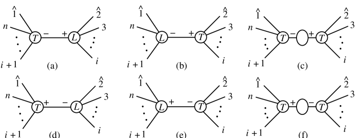
Figure 16: The recursive diagrams of the ${[1,2\rangle}$ shift for an $n$-point helicity amplitude. Some of the diagrams may vanish depending on the helicity choices.

We now discuss the recursive diagrams of the ${[1,2\rangle}$ shift, shown in fig. 16, for a generic helicity configuration. As explained in section V, we must sum over both helicities of the gluon crossing the pole, and over loop versus tree vertices appearing on either side of the pole, as well as factorization-function contributions BernChalmers in multi-particle channels. For specific helicity configurations some of the diagrams may vanish.

For the case of $A_{n;1}^{{\cal N}=0}(1^{-},2^{-},3^{-},4^{+},\ldots,n^{+})$, the recursive contributions are,

$$\hskip-8.5359ptR^{D}_{n}(1^{-},2^{-},3^{-},4^{+},\ldots,n^{+})=$$

$$\hskip 56.9055pt\sum_{i=4}^{n-1}A^{\rm tree}_{n-i+2}(\hat{1}^{-},\hat{K}_{2\ldots i}^{-},(i+1)^{+},\ldots,n^{+})\frac{i}{s_{2\ldots i}}R_{i}(\hat{2}^{-},3^{-},4^{+},\ldots,i^{+},-\hat{K}_{2\ldots i}^{+})$$

$$\hskip 42.67912pt\hbox{}+\sum_{i=4}^{n-2}R_{n-i+2}(\hat{1}^{-},\hat{K}_{2\ldots i}^{-},(i+1)^{+},\ldots,n^{+})\frac{i}{s_{2\ldots i}}A^{\rm tree}_{i}(\hat{2}^{-},3^{-},4^{+},\ldots,i^{+},-\hat{K}_{2\ldots i}^{+})$$

$$\hskip 42.67912pt\hbox{}+\sum\limits_{i=5}^{n-2}R_{n-i+2}(\hat{1}^{-},\hat{K}_{2\ldots i}^{+},(i+1)^{+},\ldots,n^{+})\frac{i}{s_{2\ldots i}}A^{\rm tree}_{i}(\hat{2}^{-},3^{-},4^{+},\ldots,i^{+},-\hat{K}_{2\ldots i}^{-})\hskip 11.38092pt$$

$$\hskip 42.67912pt\hbox{}-\Biggl{(}\frac{1}{3\epsilon}+\frac{8}{9}\Biggr{)}\sum_{i=4}^{n-2}A^{\rm tree}_{n-i+2}(\hat{1}^{-},\hat{K}_{2\ldots i}^{-},(i+1)^{+},\ldots,n^{+})\frac{i}{s_{2\ldots i}}$$

$$\hskip 113.81102pt\hbox{}\times A^{\rm tree}_{i}(\hat{2}^{-},3^{-},4^{+},\ldots,i^{+},-\hat{K}_{2\ldots i}^{+})\,,$$ (134)

where the last line comes from the factorization-function contributions. We refrain from quoting the explicit expression for $R_{n}^{D}$ here. It can be obtained straightforwardly by inserting the known tree amplitudes ParkeTaylor ; BGRecurrence ; TreeRecurResults (quoted in the appendix) and rational parts of loop amplitudes Qpap ; FordeKosower into eq. (134).

An interesting feature of this recursion relation is that all amplitudes on the right-hand side have fewer than three negative helicities. In contrast, the recursion relation found for two negative-helicity gluons Bootstrap contains on the right-hand side lower-point loop amplitudes with the same number of negative helicities as on the left-hand side, namely two. For this reason, to solve that recursion relation in closed form for all $n$ required an ‘unwinding’ procedure FordeKosower . Unwinding is not necessary in the present case because all terms on the right-hand side are known — given the two-negative-helicity solution of ref. FordeKosower .

VIII.3 Overlap Contribution

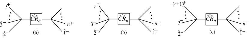
Figure 17: Overlap diagrams corresponding to the $s_{2\ldots j}$, $s_{2\ldots r}$ and $s_{2\ldots(r+1)}$ channels.

Finally, we need to compute the overlap contribution to avoid double counting between the recursive diagrams, eq. (134), and the completed-cut terms, eq. (132). First we observe that the terms proportional to the tree amplitude on the first line of eq. (132) get shifted only in the denominator, namely only in $s_{2\ldots r}$ in eq. (A). This means that the overlap contribution from this term is the negative of the term itself and thus cancels it in the full amplitude, eq. (95). Furthermore, the same happens with the term involving $\hat{h}^{{\cal N}=0}$. Thus, for these two contributions we have

$$O_{n}^{\rm tree} = -\left(\frac{1}{3\epsilon}+\frac{8}{9}\right)A_{n}^{{\rm tree}}(1^{-},2^{-},3^{-},4^{+},\ldots,n^{+})\,,$$ (135)

$$O_{n}^{\hat{h}\mbox{-}{\rm term}} = \frac{i}{6}\sum_{r=4}^{n-2}{\hat{h}_{n,r}^{{\cal N}=0}}{s_{3\ldots r}+s_{3\ldots(r+1)}\over s_{3\ldots r}s_{3\ldots(r+1)}(s_{3\ldots(r+1)}-s_{3\ldots r})^{2}}\,.$$ (136)

The $\hat{d}^{{\cal N}=0}$-term gives a contribution to the overlap,

$$O_{n}^{\hat{d}\mbox{-}{\rm term}}=-\frac{i}{6}\sum_{r=4}^{n-1}\frac{\left\langle\smash{3}{\vphantom{1}}^{-}\right|{{\raise 0.91666pt\hbox to9.20833pt{\hss/\hss}\hbox to0.0pt{\hss$K$}}_{3\ldots r}{\raise 0.97221pt\hbox to5.52084pt{\hss/\hss}\hbox to0.0pt{\hss$k$}}_{2}}\left|\smash{1}{\vphantom{1}}^{+}\right\rangle\,\left\langle\smash{3}{\vphantom{1}}^{-}\right|{{\raise 0.91666pt\hbox to9.20833pt{\hss/\hss}\hbox to0.0pt{\hss$K$}}_{3\ldots r}{\raise 0.91666pt\hbox to9.20833pt{\hss/\hss}\hbox to0.0pt{\hss$K$}}_{2\ldots r}}\left|\smash{1}{\vphantom{1}}^{+}\right\rangle^{2}\,\left\langle r\,(r+1)\right\rangle}{\left\langle\smash{2}{\vphantom{1}}^{+}\right|{{\raise 0.91666pt\hbox to9.20833pt{\hss/\hss}\hbox to0.0pt{\hss$K$}}_{2\ldots r}}\left|\smash{r}{\vphantom{1}}^{+}\right\rangle\left\langle\smash{2}{\vphantom{1}}^{+}\right|{{\raise 0.91666pt\hbox to9.20833pt{\hss/\hss}\hbox to0.0pt{\hss$K$}}_{2\ldots r}}\left|\smash{(r+1)}{\vphantom{1}}^{+}\right\rangle\,\prod\limits_{k=3}^{n}\left\langle k\,(k+1)\right\rangle\,s_{2\ldots r}s_{3\ldots r}}\,.$$ (137)

In discussing the $\hat{g}^{{\cal N}=0}$-term, we first re-index eq. (126) by letting $j\to j-3$, so the sum runs from $j=4$ to $j=r$. The $\hat{g}^{{\cal N}=0}$-term has three different kinds of poles, since $s_{2\ldots j}$, $s_{2\ldots r}$ and $s_{2\ldots(r+1)}$ are shifted,

$$z^{\rm(a)} = -\frac{s_{2\ldots j}}{\left\langle\smash{1}{\vphantom{1}}^{-}\right|{{\raise 0.91666pt\hbox to9.20833pt{\hss/\hss}\hbox to0.0pt{\hss$K$}}_{2\ldots j}}\left|\smash{2}{\vphantom{1}}^{-}\right\rangle}\,,$$

$$z^{(\rm b)} = -\frac{s_{2\ldots r}}{\left\langle\smash{1}{\vphantom{1}}^{-}\right|{{\raise 0.91666pt\hbox to9.20833pt{\hss/\hss}\hbox to0.0pt{\hss$K$}}_{2\ldots r}}\left|\smash{2}{\vphantom{1}}^{-}\right\rangle}\,,$$

$$z^{\rm(c)} = -\frac{s_{2\ldots(r+1)}}{\left\langle\smash{1}{\vphantom{1}}^{-}\right|{{\raise 0.91666pt\hbox to9.20833pt{\hss/\hss}\hbox to0.0pt{\hss$K$}}_{2\ldots(r+1)}}\left|\smash{2}{\vphantom{1}}^{-}\right\rangle}\,,$$ (138)

corresponding to the overlap diagrams in fig. 17. At first glance it may seem that for $j=r$ we obtain a double pole, since the denominator contains $s_{2\ldots r}^{2}$. However, from the numerator of the last factor in $\hat{g}^{{\cal N}=0}$, we obtain a factor $s_{2\ldots r}$, which cancels one of the factors in the denominator, and so we have again only single poles. Nevertheless, we treat the $j=r$ term separately and obtain for this contribution,

$$O_{n}^{{\rm(a),(b)};j=r}=\frac{i}{6}\sum_{r=4}^{n-2}\frac{\left\langle\smash{3}{\vphantom{1}}^{-}\right|{{\raise 0.91666pt\hbox to9.20833pt{\hss/\hss}\hbox to0.0pt{\hss$K$}}_{3\ldots r}{\raise 0.97221pt\hbox to5.52084pt{\hss/\hss}\hbox to0.0pt{\hss$k$}}_{r+1}}\left|\smash{1}{\vphantom{1}}^{+}\right\rangle\,\left\langle\smash{3}{\vphantom{1}}^{-}\right|{{\raise 0.91666pt\hbox to9.20833pt{\hss/\hss}\hbox to0.0pt{\hss$K$}}_{3\ldots r}{\raise 0.91666pt\hbox to9.20833pt{\hss/\hss}\hbox to0.0pt{\hss$K$}}_{2\ldots r}}\left|\smash{1}{\vphantom{1}}^{+}\right\rangle^{2}\,\left\langle r\,(r+1)\right\rangle}{\left\langle\smash{2}{\vphantom{1}}^{+}\right|{{\raise 0.91666pt\hbox to9.20833pt{\hss/\hss}\hbox to0.0pt{\hss$K$}}_{2\ldots r}}\left|\smash{r}{\vphantom{1}}^{+}\right\rangle\left\langle\smash{2}{\vphantom{1}}^{+}\right|{{\raise 0.91666pt\hbox to9.20833pt{\hss/\hss}\hbox to0.0pt{\hss$K$}}_{2\ldots r}}\left|\smash{(r+1)}{\vphantom{1}}^{+}\right\rangle\,\prod\limits_{k=3}^{n}\left\langle k\,(k+1)\right\rangle s_{2\ldots r}s_{3\ldots r}}\,.$$ (139)

After some straightforward algebra, we find the remaining contributions,

$$O_{n}^{\rm(a)} = \frac{i}{6}\sum_{r=5}^{n-2}\sum_{j=4}^{r-1}{\left\langle j\,(j+1)\right\rangle\over\left\langle\smash{2}{\vphantom{1}}^{+}\right|{{\raise 0.91666pt\hbox to9.20833pt{\hss/\hss}\hbox to0.0pt{\hss$K$}}_{2\ldots j}}\left|\smash{j}{\vphantom{1}}^{+}\right\rangle\left\langle\smash{2}{\vphantom{1}}^{+}\right|{{\raise 0.91666pt\hbox to9.20833pt{\hss/\hss}\hbox to0.0pt{\hss$K$}}_{2\ldots j}}\left|\smash{(j+1)}{\vphantom{1}}^{+}\right\rangle\,\prod\limits_{k=3}^{n}\left\langle k\,(k+1)\right\rangle\,s_{3\ldots j}\,s_{2\ldots j}}$$ (140)

$$\hbox{}\times{\left\langle\smash{3}{\vphantom{1}}^{-}\right|{{\raise 0.91666pt\hbox to9.20833pt{\hss/\hss}\hbox to0.0pt{\hss$K$}}_{3\ldots j}{\raise 0.91666pt\hbox to9.20833pt{\hss/\hss}\hbox to0.0pt{\hss$K$}}_{2\ldots j}}\left|\smash{1}{\vphantom{1}}^{+}\right\rangle^{3}\left\langle\smash{1}{\vphantom{1}}^{-}\right|{{\raise 0.97221pt\hbox to5.52084pt{\hss/\hss}\hbox to0.0pt{\hss$k$}}_{r+1}{\raise 0.91666pt\hbox to9.20833pt{\hss/\hss}\hbox to0.0pt{\hss$K$}}_{(j+1)\ldots r}{\raise 0.91666pt\hbox to9.20833pt{\hss/\hss}\hbox to0.0pt{\hss$K$}}_{2\ldots j}}\left|\smash{2}{\vphantom{1}}^{-}\right\rangle\left\langle\smash{1}{\vphantom{1}}^{-}\right|{{\raise 0.91666pt\hbox to9.20833pt{\hss/\hss}\hbox to0.0pt{\hss$K$}}_{2\ldots r}{\raise 0.97221pt\hbox to5.52084pt{\hss/\hss}\hbox to0.0pt{\hss$k$}}_{r+1}{\raise 0.91666pt\hbox to9.20833pt{\hss/\hss}\hbox to0.0pt{\hss$K$}}_{2\ldots j}}\left|\smash{2}{\vphantom{1}}^{-}\right\rangle\over{\left\langle\smash{1}{\vphantom{1}}^{-}\right|{({\raise 0.97221pt\hbox to5.52084pt{\hss/\hss}\hbox to0.0pt{\hss$k$}}_{r+1}{\raise 0.91666pt\hbox to9.20833pt{\hss/\hss}\hbox to0.0pt{\hss$K$}}_{(j+1)\ldots r}+{\raise 0.91666pt\hbox to9.20833pt{\hss/\hss}\hbox to0.0pt{\hss$K$}}_{2\ldots r}{\raise 0.97221pt\hbox to5.52084pt{\hss/\hss}\hbox to0.0pt{\hss$k$}}_{r+1}){\raise 0.91666pt\hbox to9.20833pt{\hss/\hss}\hbox to0.0pt{\hss$K$}}_{2\ldots j}}\left|\smash{2}{\vphantom{1}}^{-}\right\rangle}^{2}}$$

$$\hbox{}\times\Biggl{(}\frac{1}{\left\langle\smash{1}{\vphantom{1}}^{-}\right|{{\raise 0.91666pt\hbox to9.20833pt{\hss/\hss}\hbox to0.0pt{\hss$K$}}_{2\ldots j}{\raise 0.91666pt\hbox to9.20833pt{\hss/\hss}\hbox to0.0pt{\hss$K$}}_{(j+1)\ldots r}{\raise 0.91666pt\hbox to9.20833pt{\hss/\hss}\hbox to0.0pt{\hss$K$}}_{2\ldots r}}\left|\smash{2}{\vphantom{1}}^{-}\right\rangle}+\frac{1}{\left\langle\smash{1}{\vphantom{1}}^{-}\right|{{\raise 0.91666pt\hbox to9.20833pt{\hss/\hss}\hbox to0.0pt{\hss$K$}}_{2\ldots j}{\raise 0.91666pt\hbox to9.20833pt{\hss/\hss}\hbox to0.0pt{\hss$K$}}_{(j+1)\ldots(r+1)}{\raise 0.91666pt\hbox to9.20833pt{\hss/\hss}\hbox to0.0pt{\hss$K$}}_{2\ldots(r+1)}}\left|\smash{2}{\vphantom{1}}^{-}\right\rangle}\Biggr{)}$$

$$\hbox{}\times\left\langle\smash{1}{\vphantom{1}}^{-}\right|{({\raise 0.91666pt\hbox to9.20833pt{\hss/\hss}\hbox to0.0pt{\hss$K$}}_{2\ldots r}{\raise 0.97221pt\hbox to5.52084pt{\hss/\hss}\hbox to0.0pt{\hss$k$}}_{r+1}-{\raise 0.97221pt\hbox to5.52084pt{\hss/\hss}\hbox to0.0pt{\hss$k$}}_{r+1}{\raise 0.91666pt\hbox to9.20833pt{\hss/\hss}\hbox to0.0pt{\hss$K$}}_{(j+1)\ldots r}){\raise 0.91666pt\hbox to9.20833pt{\hss/\hss}\hbox to0.0pt{\hss$K$}}_{2\ldots j}}\left|\smash{2}{\vphantom{1}}^{-}\right\rangle\,,$$

$$O_{n}^{\rm(b)} = -\frac{i}{6}\sum_{r=5}^{n-2}\sum_{j=4}^{r-1}\frac{\left\langle j\,(j+1)\right\rangle}{\left\langle\smash{2}{\vphantom{1}}^{+}\right|{{\raise 0.91666pt\hbox to9.20833pt{\hss/\hss}\hbox to0.0pt{\hss$K$}}_{2\ldots j}}\left|\smash{j}{\vphantom{1}}^{+}\right\rangle\left\langle\smash{2}{\vphantom{1}}^{+}\right|{{\raise 0.91666pt\hbox to9.20833pt{\hss/\hss}\hbox to0.0pt{\hss$K$}}_{2\ldots j}}\left|\smash{(j+1)}{\vphantom{1}}^{+}\right\rangle\,\prod\limits_{k=3}^{n}\left\langle k\,(k+1)\right\rangle s_{3\ldots j}\,s_{2\ldots r}}$$

$$\hskip 2.84544pt\hbox{}\times\frac{1}{\left\langle\smash{1}{\vphantom{1}}^{-}\right|{{\raise 0.91666pt\hbox to9.20833pt{\hss/\hss}\hbox to0.0pt{\hss$K$}}_{2\ldots r}{\raise 0.91666pt\hbox to9.20833pt{\hss/\hss}\hbox to0.0pt{\hss$K$}}_{(j+1)\ldots r}\,{\raise 0.91666pt\hbox to9.20833pt{\hss/\hss}\hbox to0.0pt{\hss$K$}}_{2\ldots j}}\left|\smash{2}{\vphantom{1}}^{-}\right\rangle\left\langle\smash{1}{\vphantom{1}}^{-}\right|{{\raise 0.91666pt\hbox to9.20833pt{\hss/\hss}\hbox to0.0pt{\hss$K$}}_{2\ldots r}{\raise 0.97221pt\hbox to5.52084pt{\hss/\hss}\hbox to0.0pt{\hss$k$}}_{r+1}\,{\raise 0.91666pt\hbox to9.20833pt{\hss/\hss}\hbox to0.0pt{\hss$K$}}_{2\ldots r}}\left|\smash{2}{\vphantom{1}}^{-}\right\rangle^{2}}$$

$$\hskip 2.84544pt\hbox{}\times\Bigg{(}\left\langle\smash{3}{\vphantom{1}}^{-}\right|{{\raise 0.91666pt\hbox to9.20833pt{\hss/\hss}\hbox to0.0pt{\hss$K$}}_{3\ldots r}{\raise 0.91666pt\hbox to9.20833pt{\hss/\hss}\hbox to0.0pt{\hss$K$}}_{2\ldots r}}\left|\smash{1}{\vphantom{1}}^{+}\right\rangle\left\langle\smash{1}{\vphantom{1}}^{-}\right|{{\raise 0.91666pt\hbox to9.20833pt{\hss/\hss}\hbox to0.0pt{\hss$K$}}_{2\ldots r}{\raise 0.97221pt\hbox to5.52084pt{\hss/\hss}\hbox to0.0pt{\hss$k$}}_{r+1}{\raise 0.91666pt\hbox to9.20833pt{\hss/\hss}\hbox to0.0pt{\hss$K$}}_{2\ldots j}}\left|\smash{2}{\vphantom{1}}^{-}\right\rangle$$

$$\hskip 28.45274pt\hbox{}-\left\langle\smash{3}{\vphantom{1}}^{-}\right|{{\raise 0.97221pt\hbox to5.52084pt{\hss/\hss}\hbox to0.0pt{\hss$k$}}_{r+1}{\raise 0.91666pt\hbox to9.20833pt{\hss/\hss}\hbox to0.0pt{\hss$K$}}_{2\ldots r}}\left|\smash{1}{\vphantom{1}}^{+}\right\rangle\left\langle\smash{1}{\vphantom{1}}^{-}\right|{{\raise 0.91666pt\hbox to9.20833pt{\hss/\hss}\hbox to0.0pt{\hss$K$}}_{2\ldots r}{\raise 0.91666pt\hbox to9.20833pt{\hss/\hss}\hbox to0.0pt{\hss$K$}}_{(j+1)\ldots r}{\raise 0.91666pt\hbox to9.20833pt{\hss/\hss}\hbox to0.0pt{\hss$K$}}_{2\ldots j}}\left|\smash{2}{\vphantom{1}}^{-}\right\rangle\Bigg{)}$$

$$\hskip 2.84544pt\hbox{}\times\Bigg{(}\left\langle\smash{3}{\vphantom{1}}^{-}\right|{{\raise 0.91666pt\hbox to9.20833pt{\hss/\hss}\hbox to0.0pt{\hss$K$}}_{3\ldots r}{\raise 0.91666pt\hbox to9.20833pt{\hss/\hss}\hbox to0.0pt{\hss$K$}}_{2\ldots r}}\left|\smash{1}{\vphantom{1}}^{+}\right\rangle\left\langle\smash{1}{\vphantom{1}}^{-}\right|{{\raise 0.97221pt\hbox to5.52084pt{\hss/\hss}\hbox to0.0pt{\hss$k$}}_{r+1}{\raise 0.91666pt\hbox to9.20833pt{\hss/\hss}\hbox to0.0pt{\hss$K$}}_{(j+1)\ldots r}{\raise 0.91666pt\hbox to9.20833pt{\hss/\hss}\hbox to0.0pt{\hss$K$}}_{2\ldots j}}\left|\smash{2}{\vphantom{1}}^{-}\right\rangle$$

$$\hskip 28.45274pt\hbox{}-\left\langle\smash{3}{\vphantom{1}}^{-}\right|{{\raise 0.91666pt\hbox to9.20833pt{\hss/\hss}\hbox to0.0pt{\hss$K$}}_{3\ldots r}{\raise 0.97221pt\hbox to5.52084pt{\hss/\hss}\hbox to0.0pt{\hss$k$}}_{r+1}}\left|\smash{1}{\vphantom{1}}^{+}\right\rangle\left\langle\smash{1}{\vphantom{1}}^{-}\right|{{\raise 0.91666pt\hbox to9.20833pt{\hss/\hss}\hbox to0.0pt{\hss$K$}}_{2\ldots r}{\raise 0.91666pt\hbox to9.20833pt{\hss/\hss}\hbox to0.0pt{\hss$K$}}_{(j+1)\ldots r}{\raise 0.91666pt\hbox to9.20833pt{\hss/\hss}\hbox to0.0pt{\hss$K$}}_{2\ldots j}}\left|\smash{2}{\vphantom{1}}^{-}\right\rangle\Bigg{)}$$

$$\hskip 2.84544pt\hbox{}\times\Bigg{(}\left\langle\smash{3}{\vphantom{1}}^{-}\right|{{\raise 0.91666pt\hbox to9.20833pt{\hss/\hss}\hbox to0.0pt{\hss$K$}}_{3\ldots r}{\raise 0.91666pt\hbox to9.20833pt{\hss/\hss}\hbox to0.0pt{\hss$K$}}_{2\ldots r}}\left|\smash{1}{\vphantom{1}}^{+}\right\rangle\left\langle\smash{1}{\vphantom{1}}^{-}\right|{({\raise 0.91666pt\hbox to9.20833pt{\hss/\hss}\hbox to0.0pt{\hss$K$}}_{2\ldots r}{\raise 0.97221pt\hbox to5.52084pt{\hss/\hss}\hbox to0.0pt{\hss$k$}}_{r+1}-{\raise 0.97221pt\hbox to5.52084pt{\hss/\hss}\hbox to0.0pt{\hss$k$}}_{r+1}{\raise 0.91666pt\hbox to9.20833pt{\hss/\hss}\hbox to0.0pt{\hss$K$}}_{(j+1)\ldots r}){\raise 0.91666pt\hbox to9.20833pt{\hss/\hss}\hbox to0.0pt{\hss$K$}}_{2\ldots j}}\left|\smash{2}{\vphantom{1}}^{-}\right\rangle$$

$$\hskip 28.45274pt\hbox{}-\left\langle\smash{3}{\vphantom{1}}^{-}\right|{({\raise 0.97221pt\hbox to5.52084pt{\hss/\hss}\hbox to0.0pt{\hss$k$}}_{r+1}{\raise 0.91666pt\hbox to9.20833pt{\hss/\hss}\hbox to0.0pt{\hss$K$}}_{2\ldots r}-{\raise 0.91666pt\hbox to9.20833pt{\hss/\hss}\hbox to0.0pt{\hss$K$}}_{3\ldots r}{\raise 0.97221pt\hbox to5.52084pt{\hss/\hss}\hbox to0.0pt{\hss$k$}}_{r+1})}\left|\smash{1}{\vphantom{1}}^{+}\right\rangle\left\langle\smash{1}{\vphantom{1}}^{-}\right|{{\raise 0.91666pt\hbox to9.20833pt{\hss/\hss}\hbox to0.0pt{\hss$K$}}_{2\ldots r}{\raise 0.91666pt\hbox to9.20833pt{\hss/\hss}\hbox to0.0pt{\hss$K$}}_{(j+1)\ldots r}{\raise 0.91666pt\hbox to9.20833pt{\hss/\hss}\hbox to0.0pt{\hss$K$}}_{2\ldots j}}\left|\smash{2}{\vphantom{1}}^{-}\right\rangle\Bigg{)}\,,$$

$$O_{n}^{\rm(c)} = -\frac{i}{6}\sum_{r=5}^{n-1}\sum_{j=4}^{r-1}\frac{\left\langle j\,(j+1)\right\rangle}{\left\langle\smash{2}{\vphantom{1}}^{+}\right|{{\raise 0.91666pt\hbox to9.20833pt{\hss/\hss}\hbox to0.0pt{\hss$K$}}_{2\ldots j}}\left|\smash{j}{\vphantom{1}}^{+}\right\rangle\left\langle\smash{2}{\vphantom{1}}^{+}\right|{{\raise 0.91666pt\hbox to9.20833pt{\hss/\hss}\hbox to0.0pt{\hss$K$}}_{2\ldots j}}\left|\smash{(j+1)}{\vphantom{1}}^{+}\right\rangle\,\prod\limits_{k=3}^{n}\left\langle k\,(k+1)\right\rangle s_{3\ldots j}\,s_{2\ldots r}}\hskip 28.45274pt$$

$$\hskip 2.84544pt\hbox{}\times\frac{1}{\left\langle\smash{1}{\vphantom{1}}^{-}\right|{{\raise 0.91666pt\hbox to9.20833pt{\hss/\hss}\hbox to0.0pt{\hss$K$}}_{2\ldots r}{\raise 0.91666pt\hbox to9.20833pt{\hss/\hss}\hbox to0.0pt{\hss$K$}}_{(j+1)\ldots r}{\raise 0.91666pt\hbox to9.20833pt{\hss/\hss}\hbox to0.0pt{\hss$K$}}_{2\ldots j}}\left|\smash{2}{\vphantom{1}}^{-}\right\rangle\left\langle\smash{1}{\vphantom{1}}^{-}\right|{{\raise 0.91666pt\hbox to9.20833pt{\hss/\hss}\hbox to0.0pt{\hss$K$}}_{2\ldots r}{\raise 0.97221pt\hbox to5.52084pt{\hss/\hss}\hbox to0.0pt{\hss$k$}}_{r}{\raise 0.91666pt\hbox to9.20833pt{\hss/\hss}\hbox to0.0pt{\hss$K$}}_{2\ldots r}}\left|\smash{2}{\vphantom{1}}^{-}\right\rangle^{2}}$$

$$\hskip 2.84544pt\hbox{}\times\Bigg{(}\left\langle\smash{3}{\vphantom{1}}^{-}\right|{{\raise 0.91666pt\hbox to9.20833pt{\hss/\hss}\hbox to0.0pt{\hss$K$}}_{3\ldots r}{\raise 0.91666pt\hbox to9.20833pt{\hss/\hss}\hbox to0.0pt{\hss$K$}}_{2\ldots r}}\left|\smash{1}{\vphantom{1}}^{+}\right\rangle\left\langle\smash{1}{\vphantom{1}}^{-}\right|{{\raise 0.91666pt\hbox to9.20833pt{\hss/\hss}\hbox to0.0pt{\hss$K$}}_{2\ldots r}{\raise 0.97221pt\hbox to5.52084pt{\hss/\hss}\hbox to0.0pt{\hss$k$}}_{r}{\raise 0.91666pt\hbox to9.20833pt{\hss/\hss}\hbox to0.0pt{\hss$K$}}_{2\ldots j}}\left|\smash{2}{\vphantom{1}}^{-}\right\rangle$$

$$\hskip 28.45274pt\hbox{}-\left\langle\smash{3}{\vphantom{1}}^{-}\right|{{\raise 0.97221pt\hbox to5.52084pt{\hss/\hss}\hbox to0.0pt{\hss$k$}}_{r}{\raise 0.91666pt\hbox to9.20833pt{\hss/\hss}\hbox to0.0pt{\hss$K$}}_{2\ldots r}}\left|\smash{1}{\vphantom{1}}^{+}\right\rangle\left\langle\smash{1}{\vphantom{1}}^{-}\right|{{\raise 0.91666pt\hbox to9.20833pt{\hss/\hss}\hbox to0.0pt{\hss$K$}}_{2\ldots r}{\raise 0.91666pt\hbox to9.20833pt{\hss/\hss}\hbox to0.0pt{\hss$K$}}_{(j+1)\ldots r}{\raise 0.91666pt\hbox to9.20833pt{\hss/\hss}\hbox to0.0pt{\hss$K$}}_{2\ldots j}}\left|\smash{2}{\vphantom{1}}^{-}\right\rangle\Bigg{)}$$

$$\hskip 2.84544pt\hbox{}\times\Bigg{(}\left\langle\smash{3}{\vphantom{1}}^{-}\right|{{\raise 0.91666pt\hbox to9.20833pt{\hss/\hss}\hbox to0.0pt{\hss$K$}}_{3\ldots r}{\raise 0.91666pt\hbox to9.20833pt{\hss/\hss}\hbox to0.0pt{\hss$K$}}_{2\ldots r}}\left|\smash{1}{\vphantom{1}}^{+}\right\rangle\left\langle\smash{1}{\vphantom{1}}^{-}\right|{{\raise 0.97221pt\hbox to5.52084pt{\hss/\hss}\hbox to0.0pt{\hss$k$}}_{r}{\raise 0.91666pt\hbox to9.20833pt{\hss/\hss}\hbox to0.0pt{\hss$K$}}_{(j+1)\ldots r}{\raise 0.91666pt\hbox to9.20833pt{\hss/\hss}\hbox to0.0pt{\hss$K$}}_{2\ldots j}}\left|\smash{2}{\vphantom{1}}^{-}\right\rangle$$

$$\hskip 28.45274pt\hbox{}-\left\langle\smash{3}{\vphantom{1}}^{-}\right|{{\raise 0.91666pt\hbox to9.20833pt{\hss/\hss}\hbox to0.0pt{\hss$K$}}_{3\ldots r}{\raise 0.97221pt\hbox to5.52084pt{\hss/\hss}\hbox to0.0pt{\hss$k$}}_{r}}\left|\smash{1}{\vphantom{1}}^{+}\right\rangle\left\langle\smash{1}{\vphantom{1}}^{-}\right|{{\raise 0.91666pt\hbox to9.20833pt{\hss/\hss}\hbox to0.0pt{\hss$K$}}_{2\ldots r}{\raise 0.91666pt\hbox to9.20833pt{\hss/\hss}\hbox to0.0pt{\hss$K$}}_{(j+1)\ldots r}{\raise 0.91666pt\hbox to9.20833pt{\hss/\hss}\hbox to0.0pt{\hss$K$}}_{2\ldots j}}\left|\smash{2}{\vphantom{1}}^{-}\right\rangle\Bigg{)}$$

$$\hskip 2.84544pt\hbox{}\times\ \Bigg{(}\left\langle\smash{3}{\vphantom{1}}^{-}\right|{{\raise 0.91666pt\hbox to9.20833pt{\hss/\hss}\hbox to0.0pt{\hss$K$}}_{3\ldots r}{\raise 0.91666pt\hbox to9.20833pt{\hss/\hss}\hbox to0.0pt{\hss$K$}}_{2\ldots r}}\left|\smash{1}{\vphantom{1}}^{+}\right\rangle\left\langle\smash{1}{\vphantom{1}}^{-}\right|{({\raise 0.91666pt\hbox to9.20833pt{\hss/\hss}\hbox to0.0pt{\hss$K$}}_{2\ldots r}{\raise 0.97221pt\hbox to5.52084pt{\hss/\hss}\hbox to0.0pt{\hss$k$}}_{r}-{\raise 0.97221pt\hbox to5.52084pt{\hss/\hss}\hbox to0.0pt{\hss$k$}}_{r}{\raise 0.91666pt\hbox to9.20833pt{\hss/\hss}\hbox to0.0pt{\hss$K$}}_{(j+1)\ldots r}){\raise 0.91666pt\hbox to9.20833pt{\hss/\hss}\hbox to0.0pt{\hss$K$}}_{2\ldots j}}\left|\smash{2}{\vphantom{1}}^{-}\right\rangle$$

$$\hskip 28.45274pt\hbox{}-\left\langle\smash{3}{\vphantom{1}}^{-}\right|{({\raise 0.97221pt\hbox to5.52084pt{\hss/\hss}\hbox to0.0pt{\hss$k$}}_{r}{\raise 0.91666pt\hbox to9.20833pt{\hss/\hss}\hbox to0.0pt{\hss$K$}}_{2\ldots r}-{\raise 0.91666pt\hbox to9.20833pt{\hss/\hss}\hbox to0.0pt{\hss$K$}}_{3\ldots r}{\raise 0.97221pt\hbox to5.52084pt{\hss/\hss}\hbox to0.0pt{\hss$k$}}_{r})}\left|\smash{1}{\vphantom{1}}^{+}\right\rangle\left\langle\smash{1}{\vphantom{1}}^{-}\right|{{\raise 0.91666pt\hbox to9.20833pt{\hss/\hss}\hbox to0.0pt{\hss$K$}}_{2\ldots r}{\raise 0.91666pt\hbox to9.20833pt{\hss/\hss}\hbox to0.0pt{\hss$K$}}_{(j+1)\ldots r}{\raise 0.91666pt\hbox to9.20833pt{\hss/\hss}\hbox to0.0pt{\hss$K$}}_{2\ldots j}}\left|\smash{2}{\vphantom{1}}^{-}\right\rangle\Bigg{)}\,.$$

In term (c) we have relabeled $r+1\rightarrow r$ in the sum.

Combining the various overlap contributions from eqs. (135)–(137) and (139)–(VIII.3) gives us the complete overlap contribution,

$$O_{n}=O_{n}^{\rm tree}+O_{n}^{\hat{h}\mbox{-}{\rm term}}+O_{n}^{\hat{d}\mbox{-}{\rm term}}+O_{n}^{{\rm(a),(b)};j=r}+O_{n}^{\rm(a)}+O_{n}^{\rm(b)}+O_{n}^{\rm(c)}\,.$$ (143)

VIII.4 Assembling the Three-Negative Helicity Amplitude

The full amplitude $A_{n;1}^{{\cal N}=0}(1^{-},2^{-},3^{-},4^{+},\ldots,n^{+})$ is obtained by combining the pieces according to eq. (95). In this equation, the completed-cut terms and their large-$z$ behavior, ${\widehat{C}}_{n}(0)$ and $\mathop{\rm Inf}_{{[1,2\rangle}}{{\widehat{C}}}_{n}$, respectively, are given in eq. (124) and eq. (133). The recursive contribution $R^{D}_{n}$ is given by eq. (134), and the overlap contribution $O_{n}$ is given in eq. (143). Finally, the large-$z$ contribution $\mathop{\rm Inf}_{{[1,2\rangle}}{A_{n;1}^{{\cal N}=0}}$ is given in eq. (106).

VIII.5 Four-Negative Helicity Amplitude

The tree amplitudes for this configuration were first computed in ref. RoibanSplitHelicity , along with all split helicity configurations, $A_{n}(1^{-},2^{-},\ldots,m^{-},(m+1)^{+},\ldots,n^{+})$, where legs of like helicity are nearest neighbors in the color ordering. At one loop, the coefficients of all logarithmic terms in the split helicity amplitudes were then computed in ref. RecurCoeff . Thus, we have the completed-cut terms of the amplitude with four negative helicities. It is straightforward to subtract the spurious large-$z$ behavior of the completed-cut terms under a ${[1,2\rangle}$ shift, and to extract the overlap terms. The terms with large-$z$ behavior under the ${[1,2\rangle}$ shift are given in eq. (116), leaving only the direct recursive contributions to be computed, according to eq. (95).

The ${[1,2\rangle}$ shift recursion relation for four color-adjacent negative-helicity gluons may be read off from fig. 16,

$$\hskip-8.5359ptR^{D}_{n}(1^{-},2^{-},3^{-},4^{-},5^{+},\ldots,n^{+})=$$

$$\hskip 51.21504pt\sum_{i=4}^{n-1}A^{\rm tree}_{n-i+2}(\hat{1}^{-},\hat{K}_{2\ldots i}^{-},(i+1)^{+},\ldots,n^{+})\frac{i}{s_{2\ldots i}}R_{i}(\hat{2}^{-},3^{-},4^{-},5^{+},\ldots,i^{+},-\hat{K}_{2\ldots i}^{+})$$

$$\hskip 42.67912pt\hbox{}+\sum_{i=5}^{n-2}R_{n-i+2}(\hat{1}^{-},\hat{K}_{2\ldots i}^{-},(i+1)^{+},\ldots,n^{+})\frac{i}{s_{2\ldots i}}A^{\rm tree}_{i}(\hat{2}^{-},3^{-},4^{-},5^{+},\ldots,i^{+},-\hat{K}_{2\ldots i}^{+})$$

$$\hbox{}\hskip 42.67912pt+\sum\limits_{i=6}^{n-2}R_{n-i+2}(\hat{1}^{-},\hat{K}_{2\ldots i}^{+},(i+1)^{+},\ldots,n^{+})\frac{i}{s_{2\ldots i}}A^{\rm tree}_{i}(\hat{2}^{-},3^{-},4^{-},5^{+},\ldots,i^{+},-\hat{K}_{2\ldots i}^{-})\hskip 11.38092pt$$

$$\hbox{}\hskip 42.67912pt-\Biggl{(}\frac{1}{3\epsilon}+\frac{8}{9}\Biggr{)}\sum_{i=5}^{n-2}A^{\rm tree}_{n-i+2}(\hat{1}^{-},\hat{K}_{2\ldots i}^{-},(i+1)^{+},\ldots,n^{+})\frac{i}{s_{2\ldots i}}$$

$$\hskip 113.81102pt\hbox{}\times A^{\rm tree}_{i}(\hat{2}^{-},3^{-},4^{+},5^{+},\ldots,i^{+},-\hat{K}_{2\ldots i}^{+})\,,$$ (144)

where we omitted vanishing diagrams. We have solved this recursion relation through $n=8$. Although we will not present the analytic solution here, in section IX we present the numerical value of $A_{8;1}^{{\cal N}=0}(1^{-},2^{-},3^{-},4^{-},5^{+},6^{+},7^{+},8^{+})$ at one phase-space point.

VIII.6 Consistency of the Computed Amplitudes

In order to confirm our procedure for constructing the amplitudes, we have performed a number of checks on the amplitudes. A simple check is on the reflection symmetry of the amplitudes under a reversal of legs,

$$A_{n;1}(1^{-},2^{-},3^{-},4^{+},\ldots,n^{+})=(-1)^{n+1}A_{n;1}(3^{-},2^{-},1^{-},n^{+},\ldots,4^{+})\,,$$ (145)

and

$$A_{n;1}(1^{-},2^{-},3^{-},4^{-},5^{+},\ldots,n^{+})=(-1)^{n+1}A_{n;1}(4^{-},3^{-},2^{-},1^{-},n^{+},\ldots,5^{+})\,.$$ (146)

Our choice of shifts makes this symmetry unobvious, so confirming the symmetry provides a rather non-trivial consistency check. We have confirmed the above symmetry numerically through $n=10$ for the case with three negative helicities and at $n=8$ for the case with four negative helicities. We have also confirmed numerically that the amplitudes have the correct factorization properties with real momenta through $n=8$. We checked that all unphysical spurious poles are removable, for $n=6$ (as mentioned in section IV) and for $n=7$. These checks provide a strong confirmation that we found the correct analytic expressions for the amplitudes. Moreover, they also validate our recursive determination of the amplitudes’ large-$z$ behavior.

IX Numerical Points in Phase Space

In order to aid the future implementation of these amplitudes in numerical codes, we present values of the amplitudes at one point in phase space. We present numerics for selected helicity amplitudes up to eight points, as a demonstration of the utility of our methods for high-multiplicity processes. At six points, where independent numerical values are available EGZ06 , we can use these as an additional check on the amplitudes.

We quote the numerical results in an unrenormalized form. The renormalization amounts to carrying out the subtraction of eq. (14).

Since we have exact analytical expressions for the amplitudes, it is a simple matter to evaluate the amplitudes to arbitrary precision; we give ten significant digits. High precision can be useful for studying the properties of the amplitudes near (removable) spurious singularities, in order to investigate numerical instabilities (roundoff error, etc.) which might be encountered under phase-space integration. Because our analytic expressions possess only a relatively mild set of spurious singularities, in comparison to more direct evaluations of Feynman diagrams, we do not anticipate any significant complications arising from roundoff error when constructing an NLO program.

At six points, for ease of comparison, we choose the same numerical point as given in ref. EGZ06 .

$$k_{1} = {\mu\over 2}\,(-1,\,\sin\theta,\,\cos\theta\sin\phi,\,\cos\theta\cos\phi)\,,$$

$$k_{2} = {\mu\over 2}\,(-1,\,-\sin\theta,\,-\cos\theta\sin\phi,\,-\cos\theta\cos\phi)\,,$$

$$k_{3} = {\mu\over 3}\,(1,\,1,\,0,\,0)\,,$$

$$k_{4} = {\mu\over 7}\,(1,\,\cos\beta,\,\sin\beta,\,0)\,,$$

$$k_{5} = {\mu\over 6}\,(1,\,\cos\alpha\cos\beta,\,\cos\alpha\sin\beta,\,\sin\alpha)\,,$$

$$k_{6} = -k_{1}-k_{2}-k_{3}-k_{4}-k_{5}\,,$$ (147)

where

$$\theta={\pi\over 4}\,,\hskip 28.45274pt\phi={\pi\over 6}\,,\hskip 28.45274pt\alpha={\pi\over 3}\,,\hskip 28.45274pt\cos\beta=-{7\over 19}\,.$$ (148)

With this choice, the energies of $k_{1}$ and $k_{2}$ are negative, representing a physical scattering process at a collider. As in ref. EGZ06 , we choose $\mu=n=6$ GeV, where $\mu$ is the scale originating from the dimensionally-regulated integrals.

At seven points, we choose the kinematic point,

$$k_{1} = {\mu\over 2}\,(-1,\sin\theta,\cos\theta\sin\phi,\cos\theta\cos\phi)\,,$$

$$k_{2} = {\mu\over 2}\,(-1,-\sin\theta,-\cos\theta\sin\phi,-\cos\theta\cos\phi)\,,$$

$$k_{3} = {\mu\over 3}(1,1,0,0)\,,$$

$$k_{4} = {\mu\over 8}(1,\cos\beta,\sin\beta,0)\,,$$

$$k_{5} = {\mu\over 10}(1,\cos\alpha\cos\beta,\cos\alpha\sin\beta,\sin\alpha)\,,$$

$$k_{6} = {\mu\over 12}(1,\cos\gamma\cos\beta,\cos\gamma\sin\beta,\sin\gamma)\,,$$

$$k_{7} = -k_{1}-k_{2}-k_{3}-k_{4}-k_{5}-k_{6}\,,$$ (149)

where

$$\theta={\pi\over 4}\,,\hskip 28.45274pt\phi={\pi\over 6}\,,\hskip 28.45274pt\alpha={\pi\over 3}\,,\hskip 28.45274pt\gamma={2\pi\over 3}\,,\hskip 28.45274pt\cos\beta=-{37\over 128}\,,$$ (150)

and $\mu=7$ GeV.

At eight points we choose as our reference kinematic point ,

$$k_{1} = {\mu\over 2}(-1,\,\sin\theta,\,\cos\theta\sin\phi,\,\cos\theta\cos\phi)\,,$$

$$k_{2} = {\mu\over 2}(-1,\,-\sin\theta,\,-\cos\theta\sin\phi,\,-\cos\theta\cos\phi)\,,$$

$$k_{3} = {\mu\over 3}(1,\,1,\,0,\,0)\,,$$

$$k_{4} = {\mu\over 3}(1,\,\cos\beta,\,\sin\beta,\,0)\,,$$

$$k_{5} = {\mu\over 4}(1,\,\cos\alpha\cos\beta,\,\cos\alpha\sin\beta,\,\sin\alpha)\,,$$

$$k_{6} = {\mu\over 5}(1,\,\cos\gamma\cos\beta,\,\cos\gamma\sin\beta,\,\sin\gamma)\,,$$

$$k_{7} = {\mu\over 6}(1,\,\cos\delta\cos\beta,\,\cos\delta\sin\beta,\,\sin\delta)\,,$$

$$k_{8} = -k_{1}-k_{2}-k_{3}-k_{4}-k_{5}-k_{6}-k_{7}\,,$$ (151)

where

$$\theta={\pi\over 4}\,,\hskip 22.76228pt\phi={\pi\over 6}\,,\hskip 22.76228pt\alpha={\pi\over 3}\,,\hskip 22.76228pt\gamma={2\pi\over 3}\,,\hskip 22.76228pt\delta=-{2\pi\over 3}\,,\hskip 22.76228pt\cos\beta=-{10\over 11}\,,\hskip 28.45274pt$$ (152)

and we choose $\mu=8$ GeV.

Table 3: Numerical results for the nonvanishing ${\cal N}=4$ six- and seven-gluon split helicity amplitudes in the FDH scheme. The kinematic point is given in eqs. (147) and (149). The analytical expressions used for this table are from refs. Neq4Oneloop ; Neq1Oneloop ; NeqFourSevenPoint .

Helicity	$1/\epsilon$	$\epsilon^{0}$
${-}{-}{+}{+}{+}{+}$	$\;448.1350970+i\,288.8591589$	$\;231.6837670+i\,1219.687214$
${-}{-}{-}{+}{+}{+}$	$-\,12.83149626+i\,36.01649473\hskip 2.84544pt$	$-\,82.74583978+i\,33.53625588\hskip 2.84544pt$
${-}{-}{+}{+}{+}{+}{+}$	$2923.502435+i\,683.4723607$	$5112.775012+i\,6035.881921$
${-}{-}{-}{+}{+}{+}{+}$	$-\,45.77174817+i\,14.37948381$	$-\,118.6756853-i\,49.76271406$

Table 4: Numerical results for the nonvanishing ${\cal N}=1$ chiral contributions to six-, seven- and eight-gluon split helicity amplitudes. The kinematic point is given in eqs. (147), (149) and (151). The analytical expressions were obtained from refs. Neq1Oneloop ; NeqOneNMHVSixPt ; BBDPSQCD ; RecurCoeff .

Helicity	$1/\epsilon$	$\epsilon^{0}$
${-}{-}{+}{+}{+}{+}$	$-\,28.11035867+i\,4.643367883$	$-\,108.9419206+i\,35.02980993$
${-}{-}{-}{+}{+}{+}$	$-\,0.7843602985-i\,1.886592441$	$0.1435789412-i\,5.332008939$
${-}{-}{+}{+}{+}{+}{+}$	$-\,104.5611840+i\,45.34709475$	$-\,429.6932951+i\,209.0560823$
${-}{-}{-}{+}{+}{+}{+}$	$1.069354012-i\,1.474267821$	$1.619538641+i\,3.617458324$
${-}{-}{+}{+}{+}{+}{+}{+}$	$-\,0.1599026654-i\,0.1215536994$	$-\,0.4460113565-i\,0.2626240110$
${-}{-}{-}{+}{+}{+}{+}{+}$	$-\,0.01086792081-i\,0.002373299774$	$-\,0.003818661190-i\,0.02634017264\hskip 2.84544pt$
${-}{-}{-}{-}{+}{+}{+}{+}$	$-\,0.006820678758-i\,0.003628936145\hskip 2.84544pt$	$0.02086909214-i\,0.04355499656$

Table 5: Numerical results for the ${\cal N}=0$ scalar contributions to six-, seven- and eight-gluon split helicity amplitudes. The analytical expressions were obtained from refs. AllPlus ; Mahlon ; Neq1Oneloop ; Qpap ; Bootstrap ; FordeKosower ; RecurCoeff as well as sections IV and VIII of the present paper.

Helicity	$1/\epsilon$	$\epsilon^{0}$
${+}{+}{+}{+}{+}{+}$	$0$	$0.1024706290+i\,0.5198025397$
${-}{+}{+}{+}{+}{+}$	$0$	$2.749806130+i\,1.750985849$
${-}{-}{+}{+}{+}{+}$	$-\,9.370119558+i\,1.547789294$	$-\,45.80779561+i\,13.03695870$
${-}{-}{-}{+}{+}{+}$	$-\,0.2614534328-i\,0.6288641470$	$0.3883482043-i\,5.830791857$
${+}{+}{+}{+}{+}{+}{+}$	$0$	$0.1815778027+i\,1.941357266$
${-}{+}{+}{+}{+}{+}{+}$	$0$	$22.52927821+i\,5.464377788$
${-}{-}{+}{+}{+}{+}{+}$	$-\,34.85372799+i\,15.11569825$	$-\,176.2169235+i\,87.93931019$
${-}{-}{-}{+}{+}{+}{+}$	$0.3564513374-i\,0.4914226070$	$0.7087164424-i\,11.32916632$
${+}{+}{+}{+}{+}{+}{+}{+}$	$0$	$-\,0.0009856214410+i\,0.002143695508\hskip 2.84544pt$
${-}{+}{+}{+}{+}{+}{+}{+}$	$0$	$0.001078316199+i\,0.03129931739$
${-}{-}{+}{+}{+}{+}{+}{+}$	$-\,0.05330088846-i\,0.04051789981$	$0.05513350697+i\,0.1659518861$
${-}{-}{-}{+}{+}{+}{+}{+}$	$-0.003622640270-i\,0.0007910999246\hskip 2.84544pt$	$0.02719752089-i\,0.02586206549$
${-}{-}{-}{-}{+}{+}{+}{+}$	$-\,0.002273559586-i\,0.001209645382$	$0.01154855076-i\,0.0008935357840$

As explained in section II, it is convenient to decompose QCD amplitudes in terms of ${\cal N}=4$, ${\cal N}=1$, and ${\cal N}=0$ amplitudes. QCD amplitudes are recovered from these components using eq. (13).

We collect the numerical values of the split helicity amplitudes in Tables 3-5. We have extracted an overall factor of $ic_{\Gamma}$ from the numerical values presented in the tables. The complete set of analytic expressions for six- and seven-point ${\cal N}=4$ amplitudes was obtained in refs. Neq4Oneloop ; Neq1Oneloop ; BCF7 ; NeqFourSevenPoint . The ${\cal N}=1$ amplitudes appearing in Table 4 were computed in refs. Neq1Oneloop ; NeqOneNMHVSixPt ; BBDPSQCD ; BBCFSQCD ; RecurCoeff . The finite ${\cal N}=0$ amplitudes were obtained in refs. AllPlus ; Mahlon ; a compact representation of the amplitude with a single negative-helicity was given more recently Qpap . The logarithmic parts of the divergent amplitudes were computed in refs. Neq1Oneloop ; RecurCoeff , while the rational-function parts were determined in refs. Bootstrap ; FordeKosower and in sections IV and VIII of the present paper. Multiple analytical calculations exist for some of the split-helicity amplitudes appearing in the tables. In particular, the ${\cal N}=4$, ${\cal N}=1$, and logarithmic parts of the ${\cal N}=0$ MHV amplitudes were also computed in refs. BST ; BBSTQCD using MHV vertices CSW .

Table 3 gives the numerical values for the $1/\epsilon$ and finite terms of the ${\cal N}=4$ super-Yang-Mills theory split-helicity six- and seven-point amplitudes. We do not include the coefficients of the leading $1/\epsilon^{2}$ singularities in the tables, as these are easily extracted from the values of tree amplitudes, for any helicity configuration,

$$A^{{\cal N}=4}_{n;1}\Bigr{|}_{1/\epsilon^{2}}=-{nc_{\Gamma}\over\epsilon^{2}}A^{{\rm tree}}_{n}\,.$$ (153)

The numerical values of the tree amplitudes may be read off from the values of the $1/\epsilon$ singularities of either the ${\cal N}=1$ or the ${\cal N}=0$ loop amplitudes,

$$A^{{\cal N}=1}_{n;1}\Bigr{|}_{1/\epsilon}={c_{\Gamma}\over\epsilon}A^{{\rm tree}}_{n}\,,\hskip 56.9055ptA^{{\cal N}=0}_{n;1}\Bigr{|}_{1/\epsilon}={c_{\Gamma}\over 3\epsilon}A^{{\rm tree}}_{n}\,,$$ (154)

given in Tables 4 and 5.

We quote numerical values of the ${\cal N}=1$ and ${\cal N}=0$ amplitudes through eight points, but refrain from giving numerical values for eight-point ${\cal N}=4$ amplitudes. (The ${\cal N}=4$ amplitude with four negative helicities has not been evaluated explicitly, although it is straightforward to obtain using the methods of ref. BCFUnitarity . The general ${\cal N}=4$ $n$-point amplitudes with three negative-helicity legs may be found in ref. NeqFourNMHV .)

We have compared our numerical results for the six-point amplitudes to those found in ref. EGZ06 . After accounting for differing overall phase conventions, they agree to within the number of digits quoted in ref. EGZ06 .

X Conclusions and Outlook

In this paper we have continued the development of the on-shell unitarity-bootstrap method Bootstrap for computing complete amplitudes in non-supersymmetric gauge theories. It combines unitarity Neq4Oneloop ; Neq1Oneloop with on-shell recursion BCFRecurrence ; BCFW . It thereby systematizes an earlier unitarity-factorization bootstrap ZFourPartons used to compute the one-loop amplitudes required for $Z\rightarrow 4$ jets and $pp\rightarrow W,Z+2$ jets. In the combined approach, cut-containing pieces are obtained via unitarity, while purely rational terms are obtained via on-shell recursion. The latter terms had previously been the most difficult part of a one-loop QCD calculation. The use of an on-shell recursion reduces them to tree-like calculations.

On-shell recursion relations rely on continuations of the amplitudes to complex momenta BCFW . As discussed in refs. OnShellRecurrenceI ; Qpap ; Bootstrap , the complex factorization properties of loop amplitudes are much more subtle than those of tree-level ones. In addition to the presence of branch cuts, in loop amplitudes we encounter double and ‘unreal’ poles, present only when the momenta are complex. Unlike the situation for real momenta, there are as yet no general theorems describing how loop amplitudes factorize for complex momenta. For general helicity configurations, some continuations of the amplitudes may require such unknown factorizations. On the other hand, in general it is not possible to choose a continuation where all factorizations are known without spoiling the vanishing of the contour integral at infinity whose consideration gives rise to the recursion relation. This unhappy situation can come about because the continued amplitude may not vanish as the continuation parameter becomes large.

How, then should we avoid channels with unknown factorization, without spoiling the recursion? In this paper we provided a general strategy for avoiding these difficulties. We construct an auxiliary recursion relation to fill in information required to re-establish the contour integral and hence the primary recursion. The latter is designed to avoid channels with non-standard factorizations, even at the price of bad behavior as the continuation parameter becomes large. The auxiliary recursion supplies the terms we need to subtract from the contour integrand in order to obtain a well-defined integral and thereby a proper recursion relation. It may have channels with non-standard factorization, but is designed so that these non-standard channels will not affect the required subtraction terms.

As an illustration of these ideas, we obtained complete $n$-gluon amplitudes with a scalar in the loop and three nearest-neighbor negative helicities in the color ordering. The logarithmic parts of these amplitudes were obtained in refs. Neq1Oneloop ; RecurCoeff ; here we constructed a recursive expression for all the rational terms that appear in these amplitudes. For the six-point scalar loop amplitude $A_{6;1}^{{\cal N}=0}(1^{-},2^{-},3^{-},4^{+},5^{+},6^{+})$ we found a compact representation for the amplitude. Using the supersymmetric decomposition GGGGG , together with the previously computed ${\cal N}=4$ and ${\cal N}=1$ supersymmetric contributions Neq1Oneloop ; BCF7 ; NeqFourSevenPoint ; NeqOneNMHVSixPt ; NeqFourNMHV ; BBDPSQCD , these provide complete QCD amplitudes. As an additional illustration, we provided a recursive expression for the eight-point amplitude with four-negative helicities, $A_{8;1}^{{\cal N}=0}(1^{-},2^{-},3^{-},4^{-},5^{+},6^{+},7^{+},8^{+})$. We gave numerical values for the amplitudes (in the supersymmetric decomposition) at specific points in phase space, to use as a guide for constructing numerical programs in the future. In a companion paper we shall present all remaining $n$-point MHV amplitudes MHVQCDLoop . These calculations of high-multiplicity and indeed all-$n$ amplitudes illustrate a crucial feature of our approach: the complexity of the calculation grows only modestly as the number of external particles increases.

The continuations typically used to derive recursion relations are implemented by shifting a pair of momenta associated with external legs. We choose pairs of such shifts. Our strategy for choosing them is based on a several empirical properties of amplitudes: that under a ${[-,+\rangle}$ shift, gluon amplitudes are well behaved for large shift parameters, that the large-parameter behavior is always polynomial in the shift parameter, and that we can suppress unwanted channels with non-standard complex factorization through appropriate choice of shifts. As yet we cannot offer formal proofs of these properties. In lieu of such proofs, we have checked the computed amplitudes by verifying the stringent real-momentum factorization properties any amplitude must satisfy. The correctness of the computed amplitudes may then be seen as further evidence for the correctness of the empirical properties.

It would be useful to address some of these open formal issues, and to develop a first-principles understanding of the complex factorization properties and large-shift-parameter behavior of one-loop scattering amplitudes. Recent papers connecting tree-level on-shell recursion to the gauge theory Lagrangian VamanYao provide one possible avenue to deriving the analytic properties. Unitarity in $D$ dimensions may also assist in this formal understanding BernMorgan , as it can be used to determine rational parts of amplitudes, even though explicit computations are often cumbersome.

The methods we have presented in this paper are systematic and thus lend themselves to automation, most obviously in an analytic approach, but also plausibly in a semi-numerical one. The large number of required subprocesses in many applications of phenomenological interest makes such automation desirable. The techniques of this paper require as input the cut-containing parts of the amplitudes. Efficient, semi-automated procedures for evaluating unitarity cuts are therefore also necessary. As remarked in the introduction, there have been important developments in this direction in the past year or so, which are applicable to generic helicity configurations and external states in non-supersymmetric gauge theories, and which reduce the problem to one of residue extraction BBCFSQCD ; BFM . In particular, this approach has been used to complete the computation of all cut-containing parts of six-gluon amplitudes. These methods should work well in tandem with the ones presented here.

The empirical properties of the amplitudes are robust enough, and sufficiently broad, to allow the computation of arbitrary gluonic amplitudes. The same ideas should carry over to amplitudes with external quarks, vector bosons or Higgs particles. Beyond that, we foresee that with suitable extensions the method will also work for processes with massive particles propagating inside the loops. We are encouraged by the observation that the unitarity method applies to massive loops BernMorgan and that at tree level, the on-shell recursive approach carries over to massive theories without difficulty GloverMassive ; Massive . This extension of the on-shell bootstrap, to loop-level processes containing top quarks for example, is an open problem.

Even before such extensions to amplitudes with massive internal particles become available, however, the on-shell bootstrap method we have described is ready to tackle many of the important multi-parton next-to-leading order computations of phenomenological interest at the Large Hadron Collider.

Appendix A Previously Computed Amplitudes and Vertices

As discussed in the text, our bootstrap approach relies on using previously computed amplitudes. In this appendix we list the amplitudes that enter into our calculation. In the text, we also need the parity conjugates of the listed amplitudes, which are given by replacing $\left\langle i\,j\right\rangle\leftrightarrow\left[j\,i\right]$,

$$A_{n}(1^{h_{1}},2^{h_{2}},\ldots,n^{h_{n}})=\left[A_{n}(1^{-h_{1}},2^{-h_{2}},\ldots,n^{-h_{n}})\right]_{\left\langle i\,j\right\rangle\leftrightarrow\left[j\,i\right]}\,.$$ (155)

Some useful tree amplitudes are

$$A_{3}^{\rm tree}(1^{-},2^{-},3^{+}) = i{\left\langle 1\,2\right\rangle^{4}\over\left\langle 1\,2\right\rangle\left\langle 2\,3\right\rangle\left\langle 3\,1\right\rangle}\,,$$ (156)

$$A_{3}^{\rm tree}(1^{-},2^{+},3^{+}) = -i{\left[2\,3\right]^{4}\over\left[1\,2\right]\left[2\,3\right]\left[3\,1\right]}\,,$$ (157)

$$A_{4}^{\rm tree}(1^{-},2^{-},3^{+},4^{+}) = i{\left\langle 1\,2\right\rangle^{4}\over\left\langle 1\,2\right\rangle\left\langle 2\,3\right\rangle\left\langle 3\,4\right\rangle\left\langle 4\,1\right\rangle}\,,$$ (158)

$$A^{\rm tree}_{5}(1^{-},2^{-},3^{+},4^{+},5^{+}) = i{\left\langle 1\,2\right\rangle^{4}\over\left\langle 1\,2\right\rangle\left\langle 2\,3\right\rangle\left\langle 3\,4\right\rangle\left\langle 4\,5\right\rangle\left\langle 5\,1\right\rangle}\,,$$ (159)

$$A_{5}^{\rm tree}(1^{-},2^{-},3^{-},4^{+},5^{+}) = -i{\left[4\,5\right]^{4}\over\left[1\,2\right]\left[2\,3\right]\left[3\,4\right]\left[4\,5\right]\left[5\,1\right]}\,,$$ (160)

$$A_{6}^{\rm tree}(1^{-},2^{-},3^{-},4^{+},5^{+},6^{+}) = i{\left\langle\smash{1}{\vphantom{1}}^{-}\right|{(2+3)}\left|\smash{4}{\vphantom{1}}^{-}\right\rangle^{3}\over s_{234}\left[2\,3\right]\left[3\,4\right]\left\langle 5\,6\right\rangle\left\langle 6\,1\right\rangle\left\langle\smash{5}{\vphantom{1}}^{-}\right|{(3+4)}\left|\smash{2}{\vphantom{1}}^{-}\right\rangle}$$ (161)

$$\hskip 2.84544pt\hbox{}+i{\left\langle\smash{3}{\vphantom{1}}^{-}\right|{(4+5)}\left|\smash{6}{\vphantom{1}}^{-}\right\rangle^{3}\over s_{345}\left[2\,1\right]\left[1\,6\right]\left\langle 3\,4\right\rangle\left\langle 4\,5\right\rangle\left\langle\smash{5}{\vphantom{1}}^{-}\right|{(3+4)}\left|\smash{2}{\vphantom{1}}^{-}\right\rangle}\,.$$

(The three-point amplitudes are non-vanishing for complex momenta, even though they vanish for real momenta.) The $n$-point MHV amplitudes ParkeTaylor ; BGRecurrence , and one sequence of NMHV amplitudes TreeRecurResults , are,

$$A_{n}^{\rm tree}(1^{+},\ldots,m_{1}^{-},\ldots,m_{2}^{-},\ldots,n^{+}) = i{{\left\langle m_{1}\,m_{2}\right\rangle}^{4}\over\prod\limits_{k=1}^{n}\left\langle k\,(k+1)\right\rangle}\,,$$ (162)

$$A_{n}^{\rm tree}(1^{-},2^{-},3^{-},4^{+},\ldots,n^{+}) =$$

$$-i\sum_{r=4}^{n-1}{\left\langle\smash{3}{\vphantom{1}}^{-}\right|{{\raise 0.91666pt\hbox to9.20833pt{\hss/\hss}\hbox to0.0pt{\hss$K$}}_{3\ldots r}{\raise 0.91666pt\hbox to9.20833pt{\hss/\hss}\hbox to0.0pt{\hss$K$}}_{2\ldots r}}\left|\smash{1}{\vphantom{1}}^{+}\right\rangle^{3}\left\langle r\,(r+1)\right\rangle\over\left\langle\smash{2}{\vphantom{1}}^{+}\right|{{\raise 0.91666pt\hbox to9.20833pt{\hss/\hss}\hbox to0.0pt{\hss$K$}}_{3\ldots r}}\left|\smash{r}{\vphantom{1}}^{+}\right\rangle\left\langle\smash{2}{\vphantom{1}}^{+}\right|{{\raise 0.91666pt\hbox to9.20833pt{\hss/\hss}\hbox to0.0pt{\hss$K$}}_{3\ldots r}}\left|\smash{(r+1)}{\vphantom{1}}^{+}\right\rangle s_{2\ldots r}\,s_{3\ldots r}\prod\limits_{k=3}^{n}\left\langle k\,(k+1)\right\rangle}\,.$$

Tree amplitudes with all like-helicity gluons or only one gluon of opposite helicity vanish.

We will also need certain classes of one-loop helicity amplitudes, or rather, their rational parts $R_{n}$, defined in eq. (78). The following three-vertices with a scalar in the loop vanish,

$$R_{3}(1^{-},2^{+},-{\hat{P}}_{12}^{\pm})=0\,,$$ (164)

related to the vanishing of the corresponding splitting amplitudes for real momenta Neq4Oneloop . In principle, there are also vertices with like-helicity external legs, $R_{3}(1^{-},2^{-},-{\hat{P}}_{12}^{\pm})$ and $R_{3}(1^{+},2^{+},-{\hat{P}}_{12}^{\pm})$. However, the associated complex factorization properties are not fully understood as yet, so we avoid these channels, or suppress them in a large-$z$ limit.

For multi-particle factorizations, factorization functions can appear, as discussed in section V. For the scalar loop, the one-loop factorization function is,

$${\cal F}(K)=-\biggl{(}{1\over 3\epsilon}+{1\over 3}\ln\biggl{(}{\mu^{2}\over-K^{2}}\biggr{)}+{8\over 9}\biggr{)}\,.$$ (165)

The two-point rational “vertex” associated with this is a constant,

$$R_{\cal F}=-\biggl{(}{1\over 3\epsilon}+{8\over 9}\biggr{)}\,.$$ (166)

As discussed in section II, it is convenient to apply a supersymmetric decomposition of QCD loop amplitudes into ${\cal N}=4$, ${\cal N}=1$, and ${\cal N}=0$ (scalar loop) pieces GGGGG ; TwoQuarkThreeGluon . Just as the tree-level amplitudes with all gluons of like-helicity or all but one gluons of like-helicity vanish, so do the corresponding supersymmetric ${\cal N}=4$ and ${\cal N}=1$ amplitudes; the scalar ${\cal N}=0$ amplitudes are nonvanishing, but purely rational and finite. For the finite four-point helicity amplitudes we have BKStringBased ; TwoQuarkThreeGluon ,

$$A_{4;1}^{{\cal N}=0}(1^{+},2^{+},3^{+},4^{+}) = -i\,{c_{\Gamma}\over 3}\,{\left[1\,2\right]\left[3\,4\right]\over\left\langle 1\,2\right\rangle\left\langle 3\,4\right\rangle}\,,$$ (167)

$$A_{4;1}^{{\cal N}=0}(1^{-},2^{+},3^{+},4^{+}) = i\,{c_{\Gamma}\over 3}\,{\left\langle 2\,4\right\rangle\left[2\,4\right]^{3}\over\left[1\,2\right]\left\langle 2\,3\right\rangle\left\langle 3\,4\right\rangle\left[4\,1\right]}\,.$$ (168)

The corresponding five-point amplitudes are GGGGG ,

$$A_{5;1}^{{\cal N}=0}(1^{+},2^{+},3^{+},4^{+},5^{+}) = i{c_{\Gamma}\over 3}\,\Biggl{[}{\left[1\,2\right]\left[2\,3\right]\over\left\langle 3\,4\right\rangle\left\langle 4\,5\right\rangle\left\langle 5\,1\right\rangle}+{\left[4\,5\right]\left[5\,1\right]\over\left\langle 1\,2\right\rangle\left\langle 2\,3\right\rangle\left\langle 3\,4\right\rangle}+{\left[2\,5\right]\left[3\,4\right]\over\left\langle 1\,2\right\rangle\left\langle 3\,4\right\rangle\left\langle 5\,1\right\rangle}\Biggr{]}\,,$$

$$A_{5;1}^{{\cal N}=0}(1^{-},2^{+},3^{+},4^{+},5^{+}) = i\,{c_{\Gamma}\over 3}\,{1\over\left\langle 3\,4\right\rangle^{2}}\Biggl{[}-{\left[2\,5\right]^{3}\over\left[1\,2\right]\left[5\,1\right]}+{\left\langle 1\,4\right\rangle^{3}\left[4\,5\right]\left\langle 3\,5\right\rangle\over\left\langle 1\,2\right\rangle\left\langle 2\,3\right\rangle\left\langle 4\,5\right\rangle^{2}}-{\left\langle 1\,3\right\rangle^{3}\left[3\,2\right]\left\langle 4\,2\right\rangle\over\left\langle 1\,5\right\rangle\left\langle 5\,4\right\rangle\left\langle 3\,2\right\rangle^{2}}\Biggr{]}\,.$$

Expressions for all remaining one-loop finite amplitudes may be found in refs. AllPlus ; Mahlon ; OnShellRecurrenceI .

We make use of the following functions GGGGG to express the other, cut-containing amplitudes at loop level,

$$\mathop{\hbox{\rm K}}\nolimits_{0}(s) = {1\over\epsilon\,{(1-2\,\epsilon)}}\biggl{(}{\mu^{2}\over-s}\biggr{)}^{\epsilon}\;=\;{1\over\epsilon}\;+\;\ln\biggl{(}{\mu^{2}\over-s}\biggr{)}\;+\;2\;+\;{\cal{O}}(\epsilon)\,,$$

$$\mathop{\rm L{}}\nolimits_{0}(r) = {\ln(r)\over 1-r}\,,$$

$$\mathop{\rm L{}}\nolimits_{1}(r) = {\mathop{\rm L{}}\nolimits_{0}(r)+1\over 1-r}\,,$$

$$\mathop{\rm L{}}\nolimits_{2}(r) = {\ln(r)-(r-1/r)/2\over(1-r)^{3}}\,,$$ (171)

in order to eliminate spurious singularities for $r\rightarrow 1$ which are present in the pure cut terms.

The four-point amplitude $A_{4;1}(1^{-},2^{-},3^{+},4^{+})$ is given by,

$$A_{4;1}^{{\cal N}=4}(1^{-},2^{-},3^{+},4^{+}) = c_{\Gamma}A^{\rm tree}(1^{-},2^{-},3^{+},4^{+})\Biggl{\{}-{2\over\epsilon^{2}}\biggl{[}\biggl{(}{\mu^{2}\over-s_{12}}\biggr{)}^{\epsilon}+\biggl{(}{\mu^{2}\over-s_{23}}\biggr{)}^{\epsilon}\biggr{]}$$ (172)

$$\hskip 113.81102pt\hbox{}+\ln^{2}\biggl{(}{-s_{12}\over-s_{23}}\biggr{)}+\pi^{2}-{\delta_{R}\over 3}\Biggl{\}}\,,$$

$$A_{4;1}^{{\cal N}=1}(1^{-},2^{-},3^{+},4^{+}) = c_{\Gamma}A^{\rm tree}(1^{-},2^{-},3^{+},4^{+})\biggl{(}{1\over\epsilon}+\ln\biggl{(}{\mu^{2}\over-s_{23}}\biggr{)}+2\biggr{)}\,,$$ (173)

$$A_{4;1}^{{\cal N}=0}(1^{-},2^{-},3^{+},4^{+}) = c_{\Gamma}A^{\rm tree}(1^{-},2^{-},3^{+},4^{+})\biggl{(}{1\over 3\epsilon}+{1\over 3}\ln\biggl{(}{\mu^{2}\over-s_{23}}\biggr{)}+{8\over 9}\biggr{)}\,,$$ (174)

where the regularization-scheme parameter $\delta_{R}$ was discussed in section II. The recursive vertex we need for the ${\cal N}=0$ scalar loop contribution is therefore given by

$$R_{4}(1^{-},2^{-},3^{+},4^{+})=\biggl{(}{1\over 3\epsilon}+{8\over 9}\biggr{)}A^{\rm tree}(1^{-},2^{-},3^{+},4^{+})\,.$$ (175)

The remaining five-point amplitude with adjacent like helicities that we use is,

$$A^{{\cal N}=4}_{5;1}(1^{-},2^{-},3^{-},4^{+},5^{+}) = c_{\Gamma}A^{\rm tree}(1^{-},2^{-},3^{-},4^{+},5^{+})$$ (176)

$$\hskip-119.50157pt\times\biggl{[}-{1\over\epsilon^{2}}\sum_{j=1}^{5}\biggl{(}{\mu^{2}\over-s_{j,j+1}}\biggr{)}^{\epsilon}+\sum_{j=1}^{5}\ln\biggl{(}{-s_{j,j+1}\over-s_{j+1,j+2}}\biggr{)}\,\ln\biggl{(}{-s_{j+2,j-2}\over-s_{j-2,j-1}}\biggr{)}+{5\over 6}\pi^{2}-{\delta_{R}\over 3}\biggr{]}\,,$$

$$A^{{\cal N}=1}_{5;1}(1^{-},2^{-},3^{-},4^{+},5^{+}) =$$

$$\hskip-119.50157ptc_{\Gamma}A^{\rm tree}(1^{-},2^{-},3^{-},4^{+},5^{+})\biggl{[}{1\over 2\epsilon}\biggl{\{}\biggl{(}{\mu^{2}\over-s_{51}}\biggr{)}^{\epsilon}+\biggl{(}{\mu^{2}\over-s_{34}}\biggr{)}^{\epsilon}\biggr{\}}+2\biggr{]}$$

$$\hskip-119.50157pt-i\,{c_{\Gamma}\over 2}{{\left[4\,5\right]}^{2}\biggl{(}\left[5\,1\right]\left\langle 1\,2\right\rangle\left[2\,4\right]+\left[5\,2\right]\left\langle 2\,3\right\rangle\left[3\,4\right]\biggr{)}\over\left[1\,2\right]\left[2\,3\right]\left[3\,4\right]\left[5\,1\right]}{\mathop{\rm L{}}\nolimits_{0}\biggl{(}{-s_{51}\over-s_{34}}\biggr{)}\over s_{34}}\,,$$

$$A^{{\cal N}=0}_{5;1}(1^{-},2^{-},3^{-},4^{+},5^{+}) =$$

$$\hskip-119.50157pt{1\over 3}A^{{\cal N}=1}_{5;1}(1^{-},2^{-},3^{-},4^{+},5^{+})+{2\over 9}c_{\Gamma}A^{\rm tree}(1^{-},2^{-},3^{-},4^{+},5^{+})$$

$$\hskip-119.50157pt\hbox{}+i\,{c_{\Gamma}\over 3}{\left\langle 1\,2\right\rangle\left[2\,4\right]\left[5\,2\right]\left\langle 2\,3\right\rangle\biggl{(}\left[5\,1\right]\left\langle 1\,2\right\rangle\left[2\,4\right]+\left[5\,2\right]\left\langle 2\,3\right\rangle\left[3\,4\right]\biggr{)}\over\left[1\,2\right]\left[2\,3\right]}{\mathop{\rm L{}}\nolimits_{2}\biggl{(}{-s_{51}\over-s_{34}}\biggr{)}\over s_{34}^{3}}+c_{\Gamma}{\widehat{R}}_{5}\,,$$

where

$${\widehat{R}}_{5}=i\,\biggl{[}{1\over 3}{\left[1\,3\right]\!\left\langle 1\,3\right\rangle^{3}\over\left[1\,2\right]\!\left[2\,3\right]\!\left\langle 3\,4\right\rangle\!\left\langle 4\,5\right\rangle\!\left\langle 5\,1\right\rangle}-{1\over 3}{\left\langle 1\,3\right\rangle^{2}\left[4\,5\right]\over\left[1\,2\right]\!\left[2\,3\right]\!\left\langle 3\,4\right\rangle\!\left\langle 5\,1\right\rangle}+{1\over 6}{\left\langle 1\,2\right\rangle\!\left\langle 2\,3\right\rangle\!\left[2\,4\right]\!\left[2\,5\right]\!\left[4\,5\right]\over\left[1\,2\right]\!\left[2\,3\right]\!s_{34}s_{51}}\biggr{]}\,.$$ (179)

The vertex we need is given by setting the logarithms to zero in the amplitude,

$$R_{5}(1^{-},2^{-},3^{-},4^{+},5^{+})={1\over c_{\Gamma}}A^{{\cal N}=0}_{5;1}(1^{-},2^{-},3^{-},4^{+},5^{+})\Bigr{|}_{\ln=0}\,.$$ (180)

The ${\cal N}=4$ supersymmetric amplitude needed for constructing the complete six-point QCD amplitude with three color adjacent negative helicities is given by Neq1Oneloop ,

$$A_{6;1}^{{\cal N}=4}(1^{-},2^{-},3^{-},4^{+},5^{+},6^{+})=c_{\Gamma}\ [B_{1}\,W_{6}^{(1)}+B_{2}\,W_{6}^{(2)}+B_{3}\,W_{6}^{(3)}],$$ (181)

where

$$B_{1} = i\,{(s_{123})^{3}\over\left[1\,2\right]\left[2\,3\right]\left\langle 4\,5\right\rangle\left\langle 5\,6\right\rangle\left\langle\smash{4}{\vphantom{1}}^{-}\right|{(2+3)}\left|\smash{1}{\vphantom{1}}^{-}\right\rangle\left\langle\smash{6}{\vphantom{1}}^{-}\right|{(1+2)}\left|\smash{3}{\vphantom{1}}^{-}\right\rangle}\,,$$ (182)

$$B_{2} = i\,{\left\langle\smash{1}{\vphantom{1}}^{-}\right|{(2+3)}\left|\smash{4}{\vphantom{1}}^{-}\right\rangle^{3}\over s_{234}\left[2\,3\right]\left[3\,4\right]\left\langle 5\,6\right\rangle\left\langle 6\,1\right\rangle\left\langle\smash{5}{\vphantom{1}}^{-}\right|{(3+4)}\left|\smash{2}{\vphantom{1}}^{-}\right\rangle}$$ (183)

$$\hbox{}+i\,{\left\langle 2\,3\right\rangle^{3}\left[5\,6\right]^{3}\over s_{234}\left\langle 3\,4\right\rangle\left[6\,1\right]\left\langle\smash{4}{\vphantom{1}}^{-}\right|{(2+3)}\left|\smash{1}{\vphantom{1}}^{-}\right\rangle\left\langle\smash{2}{\vphantom{1}}^{-}\right|{(3+4)}\left|\smash{5}{\vphantom{1}}^{-}\right\rangle}\,,$$

$$B_{3} = i\,{\left\langle\smash{3}{\vphantom{1}}^{-}\right|{(1+2)}\left|\smash{6}{\vphantom{1}}^{-}\right\rangle^{3}\over s_{345}\left[6\,1\right]\left[1\,2\right]\left\langle 3\,4\right\rangle\left\langle 4\,5\right\rangle\left\langle\smash{5}{\vphantom{1}}^{-}\right|{(6+1)}\left|\smash{2}{\vphantom{1}}^{-}\right\rangle}$$ (184)

$$+i\,{\left\langle 1\,2\right\rangle^{3}\left[4\,5\right]^{3}\over s_{345}\left\langle 6\,1\right\rangle\left[3\,4\right]\left\langle\smash{6}{\vphantom{1}}^{-}\right|{(1+2)}\left|\smash{3}{\vphantom{1}}^{-}\right\rangle\left\langle\smash{2}{\vphantom{1}}^{-}\right|{(6+1)}\left|\smash{5}{\vphantom{1}}^{-}\right\rangle}\,.$$

We have taken the parity conjugate and somewhat simplified the results compared to the expression of ref. Neq1Oneloop , and used the four-dimensional helicity scheme where $\delta_{R}=0$. The combination of integral functions appearing in the amplitude is,

$$W_{6}^{(i)} = -{1\over 2\epsilon^{2}}\sum_{j=1}^{6}\left({\mu^{2}\over-s_{j(j+1)}}\right)^{\epsilon}-\ln\left({-s_{i\ldots(i+2)}\over-s_{i(i+1)}}\right)\ln\left({-s_{i\ldots(i+2)}\over-s_{(i+1)(i+2)}}\right)$$ (185)

$$-\ln\left({-s_{i\ldots(i+2)}\over-s_{(i+3)(i+4)}}\right)\ln\left({-s_{i\ldots(i+2)}\over-s_{(i+4)(i+5)}}\right)+\ln\left({-s_{i\ldots(i+2)}\over-s_{(i+2)(i+3)}}\right)\ln\left({-s_{i\ldots(i+2)}\over-s_{(i+5)i}}\right)$$

$$+{1\over 2}\ln\left({-s_{i(i+1)}\over-s_{(i+3)(i+4)}}\right)\ln\left({-s_{(i+1)(i+2)}\over-s_{(i+4)(i+5)}}\right)+{1\over 2}\ln\left({-s_{(i-1)i}\over-s_{i(i+1)}}\right)\ln\left({-s_{(i+1)(i+2)}\over-s_{(i+2)(i+3)}}\right)$$

$$+{1\over 2}\ln\left({-s_{(i+2)(i+3)}\over-s_{(i+3)(i+4)}}\right)\ln\left({-s_{(i+4)(i+5)}\over-s_{(i+5)i}}\right)+{\pi^{2}\over 3}\,.$$

References

• (1) W. T. Giele and E. W. N. Glover, JHEP 0404:029 (2004) [hep-ph/0402152];
R. K. Ellis, W. T. Giele and G. Zanderighi, Phys. Rev. D72:054018 (2005) [hep-ph/0506196].
• (2) R. K. Ellis, W. T. Giele and G. Zanderighi, Phys. Rev. D73:014027 (2006) [hep-ph/0508308].
• (3) R. K. Ellis, W. T. Giele and G. Zanderighi, JHEP 0605:027 (2006) [hep-ph/0602185].
• (4) T. Binoth, G. Heinrich and N. Kauer, Nucl. Phys. B654:277 (2003) [hep-ph/0210023];
M. Kramer and D. E. Soper, Phys. Rev. D66:054017 (2002) [hep-ph/0204113];
Z. Nagy and D. E. Soper, JHEP 0309:055 (2003) [hep-ph/0308127];
T. Binoth, J. P. Guillet, G. Heinrich, E. Pilon and C. Schubert, JHEP 0510:015 (2005) [hep-ph/0504267];
C. Anastasiou and A. Daleo, hep-ph/0511176;
M. Czakon, hep-ph/0511200;
T. Binoth, M. Ciccolini and G. Heinrich, Nucl. Phys. Proc. Suppl. 157:48 (2006) [hep-ph/0601254].
• (5) Z. Bern, L. J. Dixon, D. C. Dunbar and D. A. Kosower, Nucl. Phys. B425:217 (1994) [hep-ph/9403226].
• (6) Z. Bern, L. J. Dixon, D. C. Dunbar and D. A. Kosower, Nucl. Phys. B435:59 (1995) [hep-ph/9409265].
• (7) Z. Bern and A. G. Morgan, Nucl. Phys. B467:479 (1996) [hep-ph/9511336];
Z. Bern, L. J. Dixon, D. C. Dunbar and D. A. Kosower, Phys. Lett. B394:105 (1997) [hep-th/9611127].
• (8) Z. Bern, L. J. Dixon and D. A. Kosower, Ann. Rev. Nucl. Part. Sci.  46:109 (1996) [hep-ph/9602280];
Z. Bern, L. J. Dixon and D. A. Kosower, Nucl. Phys. Proc. Suppl.  51C:243 (1996) [hep-ph/9606378];
Z. Bern, L. J. Dixon and D. A. Kosower, JHEP 0001:027 (2000) [hep-ph/0001001];
Z. Bern, A. De Freitas and L. J. Dixon, JHEP 0203:018 (2002) [hep-ph/0201161].
• (9) F. Cachazo, P. Svrček and E. Witten, JHEP 0409:006 (2004) [hep-th/0403047];
C. J. Zhu, JHEP 0404:032 (2004) [hep-th/0403115];
G. Georgiou and V. V. Khoze, JHEP 0405:070 (2004) [hep-th/0404072];
J. B. Wu and C. J. Zhu, JHEP 0407:032 (2004) [hep-th/0406085];
J. B. Wu and C. J. Zhu, JHEP 0409:063 (2004) [hep-th/0406146];
D. A. Kosower, Phys. Rev. D71:045007 (2005) [hep-th/0406175];
G. Georgiou, E. W. N. Glover and V. V. Khoze, JHEP 0407:048 (2004) [hep-th/0407027];
Y. Abe, V. P. Nair and M. I. Park, Phys. Rev. D71:025002 (2005) [hep-th/0408191];
L. J. Dixon, E. W. N. Glover and V. V. Khoze, JHEP 0412:015 (2004) [hep-th/0411092];
Z. Bern, D. Forde, D. A. Kosower and P. Mastrolia, Phys. Rev. D72:025006 (2005) [hep-ph/0412167];
T. G. Birthwright, E. W. N. Glover, V. V. Khoze and P. Marquard, JHEP 0505:013 (2005) [hep-ph/0503063]; JHEP 0507:068 (2005) [hep-ph/0505219].
• (10) K. Risager, JHEP 0512:003 (2005) [hep-th/0508206].
• (11) A. Brandhuber, B. Spence and G. Travaglini, Nucl. Phys. B706:150 (2005) [hep-th/0407214];
C. Quigley and M. Rozali, JHEP 0501:053 (2005) [hep-th/0410278];
J. Bedford, A. Brandhuber, B. Spence and G. Travaglini, Nucl. Phys. B706:100 (2005) [hep-th/0410280].
• (12) J. Bedford, A. Brandhuber, B. Spence and G. Travaglini, Nucl. Phys. B712:59 (2005) [hep-th/0412108].
• (13) F. Cachazo, hep-th/0410077.
• (14) R. Britto, F. Cachazo and B. Feng, Phys. Rev. D71:025012 (2005) [hep-th/0410179].
• (15) F. Cachazo, P. Svrček and E. Witten, JHEP 0410:077 (2004) [hep-th/0409245].
• (16) R. Britto, F. Cachazo and B. Feng, Nucl. Phys. B725:275 (2005) [hep-th/0412103].
• (17) A. Brandhuber, S. McNamara, B. Spence and G. Travaglini, JHEP 0510:011 (2005) [hep-th/0506068];
C. Quigley and M. Rozali, JHEP 0603:004 (2006) [hep-ph/0510148].
• (18) R. Britto, E. Buchbinder, F. Cachazo and B. Feng, Phys. Rev. D72:065012 (2005) [hep-ph/0503132].
• (19) R. Britto, B. Feng and P. Mastrolia, Phys. Rev. D73:105004 (2006) [hep-ph/0602178].
• (20) Z. Bern, L. J. Dixon and D. A. Kosower, Nucl. Phys. B513:3 (1998) [hep-ph/9708239].
• (21) Z. Bern, L. J. Dixon and D. A. Kosower, JHEP 0408:012 (2004) [hep-ph/0404293].
• (22) Z. Bern, V. Del Duca, L. J. Dixon and D. A. Kosower, Phys. Rev. D71:045006 (2005) [hep-th/0410224].
• (23) R. E. Cutkosky, J. Math. Phys.  1:429 (1960);
R. J. Eden, P. V. Landshoff, D. I. Olive, J. C. Polkinghorne, The Analytic S Matrix, (Cambridge University Press, 1966).
• (24) S. J. Bidder, N. E. J. Bjerrum-Bohr, L. J. Dixon and D. C. Dunbar, Phys. Lett. B606:189 (2005) [hep-th/0410296].
• (25) S. J. Bidder, N. E. J. Bjerrum-Bohr, D. C. Dunbar and W. B. Perkins, Phys. Lett. B608:151 (2005) [hep-th/0412023].
• (26) Z. Bern, N. E. J. Bjerrum-Bohr, D. C. Dunbar and H. Ita, JHEP 0511:027 (2005) [hep-ph/0507019].
• (27) Z. Bern, L. J. Dixon and D. A. Kosower, Phys. Rev. D73:065013 (2006) [hep-ph/0507005].
• (28) R. Britto, F. Cachazo and B. Feng, Nucl. Phys. B715:499 (2005) [hep-th/0412308].
• (29) R. Britto, F. Cachazo, B. Feng and E. Witten, Phys. Rev. Lett. 94:181602 (2005) [hep-th/0501052].
• (30) Z. Bern, L. J. Dixon and D. A. Kosower, Phys. Rev. D71:105013 (2005) [hep-th/0501240].
• (31) Z. Bern, L. J. Dixon and D. A. Kosower, Phys. Rev. D72:125003 (2005) [hep-ph/0505055].
• (32) D. Forde and D. A. Kosower, Phys. Rev. D73:061701 (2006) [hep-ph/0509358].
• (33) F. A. Berends and W. T. Giele, Nucl. Phys. B306:759 (1988).
• (34) D. A. Kosower, Nucl. Phys. B335:23 (1990).
• (35) F. Caravaglios and M. Moretti, Phys. Lett. B358:332 (1995) [hep-ph/9507237];
P. Draggiotis, R. H. P. Kleiss and C. G. Papadopoulos, Phys. Lett. B439:157 (1998) [hep-ph/9807207];
F. Caravaglios, M. L. Mangano, M. Moretti and R. Pittau, Nucl. Phys. B539:215 (1999) [hep-ph/9807570].
• (36) T. Stelzer and W. F. Long, Comput. Phys. Commun.  81:357 (1994) [hep-ph/9401258].
• (37) Z. Bern, L. J. Dixon and D. A. Kosower, Phys. Rev. D72:045014 (2005) [hep-th/0412210].
• (38) R. Roiban, M. Spradlin and A. Volovich, Phys. Rev. Lett. 94:102002 (2005) [hep-th/0412265].
• (39) W. T. Giele and E. W. N. Glover, Phys. Rev. D46:1980 (1992);
Z. Kunszt, A. Signer and Z. Trócsányi, Nucl. Phys. B420:550 (1994) [hep-ph/9401294];
S. Catani, Phys. Lett. B427:161 (1998) [hep-ph/9802439].
• (40) I. Bena, Z. Bern and D. A. Kosower, Phys. Rev. D71:045008 (2005) [hep-th/0406133].
• (41) M. Dinsdale, M. Ternick and S. Weinzierl, JHEP 0603:056 (2006) [hep-ph/0602204].
• (42) J. Bedford, A. Brandhuber, B. Spence and G. Travaglini, Nucl. Phys. B721:98 (2005) [hep-th/0502146];
F. Cachazo and P. Svrček, hep-th/0502160;
N. E. J. Bjerrum-Bohr, D. C. Dunbar, H. Ita, W. B. Perkins and K. Risager, JHEP 0601:009 (2006) [hep-th/0509016].
• (43) M. Luo and C. Wen, JHEP 0503:004 (2005) [hep-th/0501121].
• (44) S. D. Badger, E. W. N. Glover, V. V. Khoze and P. Svrček, JHEP 0507:025 (2005) [hep-th/0504159].
• (45) S. D. Badger, E. W. N. Glover and V. V. Khoze, JHEP 0601:066 (2006) [hep-th/0507161];
D. Forde and D. A. Kosower, Phys. Rev. D73:065007 (2006) [hep-th/0507292];
C. Schwinn and S. Weinzierl, JHEP 0603:030 (2006) [hep-th/0602012];
P. Ferrario, G. Rodrigo and P. Talavera, Phys. Rev. Lett. 96:182001 (2006) [hep-th/0602043].
• (46) E. Witten, Commun. Math. Phys.  252:189 (2004) [hep-th/0312171];
R. Roiban, M. Spradlin and A. Volovich, JHEP 0404:012 (2004) [hep-th/0402016];
R. Roiban and A. Volovich, Phys. Rev. Lett.  93:131602 (2004) [hep-th/0402121];
R. Roiban, M. Spradlin and A. Volovich, Phys. Rev. D70:026009 (2004) [hep-th/0403190];
F. Cachazo and P. Svrček, in Proceedings of the RTN Winter School on Strings, Supergravity and Gauge Theories, edited by M. Bertolini et al. (Proceedings of Science, 2005) [hep-th/0504194].
• (47) C. F. Berger, Z. Bern, L. J. Dixon, D. Forde and D. A. Kosower, hep-ph/0607014.
• (48) Z. Bern, L. J. Dixon and D. A. Kosower, Phys. Rev. Lett.  70:2677 (1993) [hep-ph/9302280].
• (49) S. J. Bidder, N. E. J. Bjerrum-Bohr, D. C. Dunbar and W. B. Perkins, Phys. Lett. B612:75 (2005) [hep-th/0502028].
• (50) F. A. Berends, R. Kleiss, P. De Causmaecker, R. Gastmans and T. T. Wu, Phys. Lett. B103:124 (1981);
P. De Causmaecker, R. Gastmans, W. Troost and T. T. Wu, Nucl. Phys. B206:53 (1982);
Z. Xu, D. H. Zhang and L. Chang, TUTP-84/3-TSINGHUA;
R. Kleiss and W. J. Stirling, Nucl. Phys. B262:235 (1985);
J. F. Gunion and Z. Kunszt, Phys. Lett. B161:333 (1985);
Z. Xu, D. H. Zhang and L. Chang, Nucl. Phys. B291:392 (1987).
• (51) M. L. Mangano and S. J. Parke, Phys. Rept. 200:301 (1991);
L. J. Dixon, in QCD & Beyond: Proceedings of TASI ’95, ed. D. E. Soper (World Scientific, 1996) [hep-ph/9601359].
• (52) J. E. Paton and H. M. Chan, Nucl. Phys. B10:516 (1969);
P. Cvitanović, P. G. Lauwers and P. N. Scharbach, Nucl. Phys. B186:165 (1981);
D. Kosower, B. H. Lee and V. P. Nair, Phys. Lett. B201:85 (1988).
• (53) F. A. Berends and W. Giele, Nucl. Phys. B294:700 (1987).
• (54) M. L. Mangano, S. J. Parke and Z. Xu, Nucl. Phys. B298:653 (1988).
• (55) Z. Bern and D. A. Kosower, Nucl. Phys. B362:389 (1991).
• (56) G. ’t Hooft and M. Veltman, Nucl. Phys. B44:189 (1972).
• (57) Z. Bern and D. A. Kosower, Nucl. Phys. B379:451 (1992).
• (58) S. Catani, M. H. Seymour and Z. Trócsányi, Phys. Rev. D55:6819 (1997) [hep-ph/9610553];
Z. Bern, A. De Freitas, L. J. Dixon and H. L. Wong, Phys. Rev. D66:085002 (2002) [hep-ph/0202271].
• (59) Z. Bern and G. Chalmers, Nucl. Phys. B447:465 (1995) [hep-ph/9503236].
• (60) Z. Bern, V. Del Duca and C. R. Schmidt, Phys. Lett. B445:168 (1998) [hep-ph/9810409];
Z. Bern, V. Del Duca, W. B. Kilgore and C. R. Schmidt, Phys. Rev. D60:116001 (1999) [hep-ph/9903516].
• (61) D. A. Kosower, Nucl. Phys. B552:319 (1999) [hep-ph/9901201];
D. A. Kosower and P. Uwer, Nucl. Phys. B563:477 (1999) [hep-ph/9903515].
• (62) P. D. Draggiotis, R. H. P. Kleiss, A. Lazopoulos and C. G. Papadopoulos, hep-ph/0511288;
D. Vaman and Y. P. Yao, JHEP 0604:030 (2006) [hep-th/0512031].
• (63) Z. Kunszt, A. Signer and Z. Trócsányi, Nucl. Phys. B411:397 (1994) [hep-ph/9305239].
• (64) Z. Kunszt, A. Signer and Z. Trócsányi, Phys. Lett. B336:529 (1994) [hep-ph/9405386].
• (65) Z. Bern, L. J. Dixon and D. A. Kosower, Nucl. Phys. B437:259 (1995) [hep-ph/9409393].
• (66) Z. Bern, L. J. Dixon and D. A. Kosower, hep-th/9311026;
Z. Bern, G. Chalmers, L. J. Dixon and D. A. Kosower, Phys. Rev. Lett. 72:2134 (1994) [hep-ph/9312333].
• (67) G. Mahlon, Phys. Rev. D49:4438 (1994) [hep-ph/9312276].
• (68) R. Britto, B. Feng, R. Roiban, M. Spradlin and A. Volovich, Phys. Rev. D71:105017 (2005) [hep-th/0503198].
• (69) S. J. Parke and T. R. Taylor, Phys. Rev. Lett. 56:2459 (1986).