Probing the convergence of perturbative series in baryon
chiral perturbation theory

Abstract

Using the examples of pion-nucleon scattering and the nucleon mass we analyze the convergence of perturbative series in the framework of baryon chiral perturbation theory. For both cases we sum up sets of an infinite number of diagrams by solving equations exactly and compare the solutions with the perturbative contributions.

I Introduction

Nowadays, mesonic chiral perturbation theory (ChPT) Weinberg:1979kz ; Gasser:1984gg ; Gasser:1984yg is widely accepted as the low-energy theory of the strong interactions based on the underlying symmetries of QCD. Impressive accuracy in the description of data has been achieved in the last decade Colangelo:2000jc ; Colangelo:2001df ; Caprini:2003ta ; Caprini:2005an ; Caprini:2005zr ; Colangelo:2005cq ; Scherer:2005ki ; Bijnens:2006zp . On the other hand, the baryon sector of ChPT proved to be more problematic Gasser:1988rb . Although there has been considerable progress in recent years (see, e.g., Scherer:2002tk ), the issue of the convergence of perturbative calculations in the nucleon sector of the effective theory is still of great interest.

To compare lattice calculations with experimental data, one has to extrapolate the results to physical quark masses. The preferred method to cope with this problem is to calculate the physical quantities as functions of the quark masses in an effective field-theoretical approach (see, e.g., Beane:2004ks ; Procura:2003ig ; Leinweber:2005cm ; Procura:2006bj ). Of course, these effective theories have a limited range of applicability. The aim of this work is to probe the issue of convergence of perturbative calculations in BChPT. To that end we consider the contribution of particular infinite sets of diagrams to the $\pi N$ scattering amplitude and to the nucleon self-energy. These contributions are summed up by solving integral equations analytically. For a related analysis of exact solutions to the Bethe-Salpeter equations in BChPT in the $SU(3)$ sector, see Ref. Lutz:2001yb .

Throughout this paper we use dimensional regularization in combination with the infrared renormalization scheme Becher:1999he ; Schindler:2003xv without explicitly showing the counter-terms responsible for the subtractions of loop diagrams.

II Pion-nucleon scattering

First, let us specify the Lagrangians required for the purposes of this work. From the mesonic sector we need the lowest-order Lagrangian of the $SU(2)$ sector Gasser:1984yg

$${\cal L}_{2}=\frac{F^{2}}{4}\mbox{Tr}(\partial_{\mu}U\partial^{\mu}U^{\dagger})+\frac{F^{2}M^{2}}{4}\mbox{Tr}(U^{\dagger}+U),$$ (1)

where $U$ is a unimodular unitary matrix containing the Goldstone boson fields. In Eq. (1), $F$ denotes the pion-decay constant in the chiral limit: $F_{\pi}=F[1+{\cal O}(\hat{m})]=92.4$ MeV. Here, we work in the isospin-symmetric limit $m_{u}=m_{d}=\hat{m}$, and the lowest-order expression for the squared pion mass is $M^{2}=2B\hat{m}$, where $B$ is related to the quark condensate $\langle\bar{q}q\rangle_{0}$ in the chiral limit Gasser:1984yg . Next, the nucleon fields are collected in an isospin doublet

$$\Psi=\left(\begin{array}[]{c}p\\ n\end{array}\right)$$

with two four-component Dirac fields $p$ and $n$ describing the proton and neutron, respectively. From the nucleon sector we need the leading-order Lagrangian omitting external sources

$${\cal L}_{\pi N}^{(1)}=\bar{\Psi}\left(i\gamma_{\mu}D^{\mu}-m+\frac{1}{2}\stackrel{{\scriptstyle\circ}}{{g_{A}}}\gamma_{\mu}\gamma_{5}u^{\mu}\right)\Psi,$$ (2)

where

$$D_{\mu}\Psi=(\partial_{\mu}+\Gamma_{\mu})\Psi,\quad u^{2}=U,\quad u_{\mu}=iu^{\dagger}\partial_{\mu}Uu^{\dagger},\quad\Gamma_{\mu}=\frac{1}{2}[u^{\dagger},\partial_{\mu}u],$$

and $m$ and $\stackrel{{\scriptstyle\circ}}{{g_{A}}}$ refer to the chiral limit of the physical nucleon mass and the axial-vector coupling constant.

Let us consider elastic $\pi N$ scattering with $p_{1}$, $q_{1}$ the four-momenta of the incoming and $p_{2}$, $q_{2}$ the four-momenta of the outgoing nucleons and pions, respectively (see Fig. 1). The corresponding vertex function (amputated Green’s function) can be obtained by solving the integral equation

$$\Gamma^{ba}\left(p_{2},q_{2};p_{1},q_{1}\right) = V^{ba}\left(p_{2},q_{2};p_{1},q_{1}\right)$$ (3)

$$+ \int\frac{d^{n}k}{(2\,\pi)^{n}}\,V^{bc}\left(p_{2},q_{2};p-k,k\right)\,G(p-k,k)\,\Gamma^{ca}\left(p-k,k;p_{1},q_{1}\right)\,,$$

where $p=p_{1}+q_{1}$. $V^{ba}$ stands for the $\pi N$ effective potential and $G(p-k,k)$ is the product of the (dressed) nucleon and pion propagators. Here, the effective potential is defined as the sum of all diagrams contributing to the vertex function, which cannot be reduced to two $\pi N$ scattering diagrams by cutting one pion line and one nucleon line.

The standard representation for the vertex function in terms of isospin symmetric and antisymmetric parts reads

$$\Gamma^{ba}=\delta^{ba}\,\Gamma^{+}+\frac{1}{2}\,\left[\tau^{b},\tau^{a}\right]\,\Gamma^{-}\,.$$ (4)

For our purposes it is convenient to decompose the scattering amplitude in isospin-invariant components

$$\Gamma^{3/2} = \Gamma^{+}-\Gamma^{-}\,,$$

$$\Gamma^{1/2} = \Gamma^{+}+2\,\Gamma^{-}\,.$$ (5)

These vertex functions satisfy the integral equations written symbolically as

$$\Gamma^{I}=V^{I}+V^{I}\,G\,\Gamma^{I}\,,$$ (6)

where $I=1/2$ or $3/2$ and

$$V^{3/2} = V^{+}-V^{-}\,,$$

$$V^{1/2} = V^{+}+2\,V^{-}\,.$$

$$V^{ba} = \delta^{ba}\,V^{+}+\frac{1}{2}\,\left[\tau^{b},\tau^{a}\right]\,V^{-}\,.$$ (7)

Suppose the potential can be written as

$$V^{I}\left(p_{2},q_{2};p_{1},q_{1}\right)=\left(\begin{array}[]{cc}1&q_{2}/\\ \end{array}\right)\left(\begin{array}[]{cc}v_{11}^{I}&v_{12}^{I}\\ v_{21}^{I}&v_{22}^{I}\\ \end{array}\right)\left(\begin{array}[]{c}1\\ q_{1}/\\ \end{array}\right)\,,$$ (8)

where the $v^{I}_{ij}$ depend only on $p=p_{1}+q_{1}=p_{2}+q_{2}$ as is the case, e.g., for the potential

$$V^{ba}\left(p_{2},q_{2};p_{1},q_{1}\right)=-\frac{\epsilon^{bac}\tau^{c}}{4\,F^{2}}\,\left(q_{1}/\hskip 1.00006pt+q_{2}/\hskip 1.00006pt\right)-\frac{i\,\stackrel{{\scriptstyle\circ}}{{g_{A}}}^{2}\,\tau^{b}\tau^{a}}{4\,F^{2}}\,\frac{q_{2}/\hskip 1.00006pt\,\left(p/\hskip 1.00006pt-m\right)\,q_{1}/\hskip 1.00006pt}{p^{2}-m^{2}}\,.$$ (9)

In this case the vertex functions $\Gamma^{I}$ can also be written as

$$\Gamma^{I}\left(p_{2},q_{2};p_{1},q_{1}\right)=\left(\begin{array}[]{cc}1&q_{2}/\\ \end{array}\right)\left(\begin{array}[]{cc}\tau_{11}^{I}&\tau_{12}^{I}\\ \tau_{21}^{I}&\tau_{22}^{I}\\ \end{array}\right)\left(\begin{array}[]{c}1\\ q_{1}/\\ \end{array}\right)\,.$$ (10)

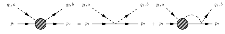
Figure 1: Equation for the pion-nucleon scattering amplitude.

Substituting Eqs. (8) and (10) in Eq. (6) results in the following matrix equations

$$\tau^{I}=v^{I}+i\,v^{I}\,g\,\tau^{I}\,,$$ (11)

where

$$g=i\int\frac{d^{n}k}{(2\,\pi)^{n}}\,\left(\begin{array}[]{c}1\\ k/\\ \end{array}\right)\,G(p-k,k)\,\left(\begin{array}[]{cc}1&k/\\ \end{array}\right)=\left(\begin{array}[]{cc}g_{11}&g_{12}\\ g_{21}&g_{22}\\ \end{array}\right)\,.$$ (12)

For the undressed propagator

$$G(p-k,k)=\frac{i}{p/\hskip 1.00006pt-k/\hskip 1.00006pt-m+i\,0^{+}}\,\frac{i}{k^{2}-M^{2}+i\,0^{+}}\,,$$ (13)

we obtain

$$g_{11} = m\,I_{N\pi}(-p,0)+p/\hskip 1.00006pt\,\left[I_{N\pi}(-p,0)-I_{N\pi}^{(p)}(-p,0)\right]\,,$$

$$g_{12} = g_{21}=\left(p^{2}+m\,p/\hskip 1.00006pt\right)\,I_{N\pi}^{(p)}(-p,0)-M^{2}\,I_{N\pi}(-p,0)-I_{N}\,,$$

$$g_{22} = p/\hskip 1.00006pt\,\left(p^{2}-m^{2}\right)\,I_{N\pi}^{(p)}(-p,0)-M^{2}\left(p/\hskip 1.00006pt-m\right)\,I_{N\pi}(-p,0)-\left(p/\hskip 1.00006pt-m\right)\,I_{N}\,.$$ (14)

The loop integrals $I_{N\pi}(-p,0)$, $I_{N}$, and $I_{N\pi}^{(p)}(-p,0)$ are given in the appendix.

Decomposing the matrices as

$$v^{I} = v_{s}^{I}+p/\hskip 1.00006pt\,v_{v}^{I}\,,$$

$$g = g_{s}+p/\hskip 1.00006pt\,g_{v}\,,$$

$$\tau^{I} = \tau_{s}^{I}+p/\hskip 1.00006pt\,\tau_{v}^{I}\,,$$ (15)

and substituting the result in Eq. (11) we obtain

$$\tau^{I}_{s} = v^{I}_{s}+i\,v^{I}_{s}\,g_{s}\,\tau^{I}_{s}+i\,p^{2}\,v^{I}_{s}\,g_{v}\,\tau^{I}_{v}+i\,p^{2}\,v^{I}_{v}\,g_{s}\,\tau^{I}_{v}+i\,p^{2}\,v^{I}_{v}\,g_{v}\,\tau^{I}_{s}\,,$$

$$\tau^{I}_{v} = v^{I}_{v}+i\,v^{I}_{v}\,g_{s}\,\tau^{I}_{s}+i\,v^{I}_{s}\,g_{v}\,\tau^{I}_{s}+i\,v^{I}_{s}\,g_{s}\,\tau^{I}_{v}+i\,p^{2}\,v^{I}_{v}\,g_{v}\,\tau^{I}_{v}\,.$$ (16)

If we define

$$v^{I}_{\pm} = v_{s}^{I}\pm\sqrt{p^{2}}\,v_{v}^{I}\,,$$

$$g_{\pm} = g_{s}\pm\sqrt{p^{2}}\,g_{v}\,,$$

$$\tau^{I}_{\pm} = \tau_{s}^{I}\pm\sqrt{p^{2}}\,\tau_{v}^{I}\,,$$ (17)

and substitute in Eq. (16) the resulting equations reduce to the decoupled system

$$\tau^{I}_{\pm}=v^{I}_{\pm}+i\,v^{I}_{\pm}\,g_{\pm}\,\tau^{I}_{\pm}\,.$$ (18)

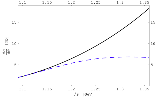
Figure 2: Differential cross section for $\pi^{-}p\to\pi^{0}n$ scattering in forward direction. The solid and dashed lines correspond to the non-perturbative and perturbative (tree plus one-loop order) results, respectively.

Eqs. (16) and (18) are systems of matrix equations and can be solved exactly. Inserting the solutions in

$$\tau^{+}_{s} = \frac{1}{3}\,\left(2\,\tau^{3/2}_{s}+\tau^{1/2}_{s}\right)\,,$$

$$\tau^{+}_{v} = \frac{1}{3}\,\left(2\,\tau^{3/2}_{v}+\tau^{1/2}_{v}\right)\,,$$

$$\tau^{-}_{s} = \frac{1}{3}\,\left(\tau^{1/2}_{s}-\tau^{3/2}_{s}\right)\,,$$

$$\tau^{-}_{v} = \frac{1}{3}\,\left(\tau^{1/2}_{v}-\tau^{3/2}_{v}\right)\,,$$ (19)

and using the most general parity-conserving form for the on-shell $T$ matrix,

$$T^{\pm}=A^{\pm}+\frac{1}{2}\,\left(q_{1}/\hskip 1.00006pt+q_{2}/\hskip 1.00006pt\right)\,B^{\pm}\,,$$ (20)

one can calculate the four Lorentz-invariant amplitudes as

$$A^{\pm} = \tau^{\pm}_{s;11}+\left(M^{2}+2\,p_{1}\cdot q_{1}\right)\,\tau^{\pm}_{s;22}+m_{N}\,\tau^{\pm}_{v;11}+2\,\left(M^{2}+2\,p_{1}\cdot q_{1}\right)\,\tau^{\pm}_{v;12}$$

$$-m_{N}\,\left(M^{2}+2\,p_{1}\cdot q_{1}\right)\,\tau^{\pm}_{v;22}\,,$$

$$B^{\pm} = 2\,\tau^{\pm}_{s;12}-2\,m_{N}\,\tau^{\pm}_{s;22}+\tau^{\pm}_{v;11}-2\,m_{N}\,\tau_{v;12}^{\pm}+\left(2\,m_{N}^{2}+M^{2}+2\,p_{1}\cdot q_{1}\right)\,\tau^{\pm}_{v;22}\,.$$ (21)

On the other hand by expanding Eqs. (21) perturbatively we can compare the results of the term-by-term loop expansion with the non-perturbative expression and estimate the error of the perturbative approximation for various kinematics.

We calculated exactly (as closed expressions of one-loop integrals) the non-perturbative (re-summed) contribution and the tree plus one-loop order contributions to the $\pi^{-}p\to\pi^{0}n$, $\pi^{-}p\to\pi^{-}p$, and $\pi^{+}p\to\pi^{+}p$ scattering processes for the potential due to the Weinberg-Tomozawa term,

$$V^{ba}\left(p_{2},q_{2};p_{1},q_{1}\right)=-\frac{\epsilon^{bac}\tau^{c}}{4\,F^{2}}\,\left(q_{1}/\hskip 1.00006pt+q_{2}/\hskip 1.00006pt\right)\,.$$ (22)

The results for differential cross sections are given in Figs. 2-4. These figures suggest that the perturbative results (tree plus one-loop order) approximate the re-summed contributions very poorly already for $s=p^{2}\sim m_{\Delta}^{2}$.

Figure 3: The sum of the differential cross sections for the processes $\pi^{-}p\to\pi^{-}p$ and $\pi^{-}p\to\pi^{0}n$ in forward direction. The solid and dashed lines correspond to the non-perturbative and perturbative (tree plus one-loop order) results, respectively.

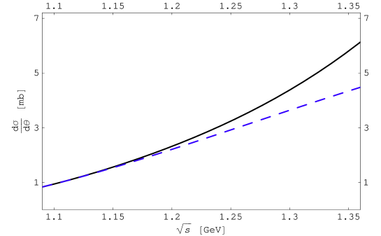
Figure 4: Differential cross section for $\pi^{+}p\to\pi^{+}p$ scattering in forward direction. The solid and dashed lines correspond to the non-perturbative and perturbative (tree plus one-loop order) results, respectively.

III Nucleon self-energy

The full (dressed) nucleon propagator has the form

$$i\,S(p)=\frac{i}{p/\hskip 1.00006pt-m-\Sigma(p/\hskip 1.00006pt)}\,,$$ (23)

where the nucleon self-energy $-i\Sigma(p/\hskip 1.00006pt)$ represents the one-particle-irreducible contribution to the two-point function. The nucleon self-energy contains the contributions of counter-terms so that $m$ corresponds to the nucleon pole mass in the chiral limit.

The physical mass $m_{N}$ of the nucleon is defined as the solution to the equation

$$S^{-1}\left(m_{N}\right)=m_{N}-m-\Sigma\left(m_{N}\right)=0\,.$$ (24)

Below we calculate the contribution to the nucleon mass of an infinite number of diagrams shown in Fig. 5. The sum of these diagrams can be written in a closed form as

$$-i\,\Sigma = -\frac{\stackrel{{\scriptstyle\circ}}{{g_{A}}}^{2}}{4\,F^{2}}\,\int\int\frac{d^{n}q_{1}}{(2\,\pi)^{n}}\,\frac{d^{n}q_{2}}{(2\,\pi)^{n}}$$ (25)

$$\times\,\gamma^{5}\,q_{2}/\hskip 1.00006pt\ \frac{1}{p/\hskip 1.00006pt-q_{2}/\hskip 1.00006pt-m_{N}}\ \tau^{b}\ \Gamma^{ba}\left(p_{2}-q_{2},q_{2};p_{1}-q_{1},q_{1}\right)\ \tau^{a}\ \frac{1}{p/\hskip 1.00006pt-q_{1}/\hskip 1.00006pt-m_{N}}\ \gamma^{5}q_{1}/\hskip 1.00006pt\$$

$$\times\,\frac{1}{\left[q_{1}^{2}-M^{2}+i\,0^{+}\right]\left[q_{2}^{2}-M^{2}+i\,0^{+}\right]}\,,$$

where the $\pi N$ vertex function $\Gamma^{ba}$ is obtained by solving Eq. (3) with the potential

$$V^{ba}\left(p_{2},q_{2};p_{1},q_{1}\right)=-\frac{\epsilon^{bac}\tau^{c}}{4\,F^{2}}\,\left(q_{1}/\hskip 1.00006pt+q_{2}/\hskip 1.00006pt\right)\,.$$ (26)

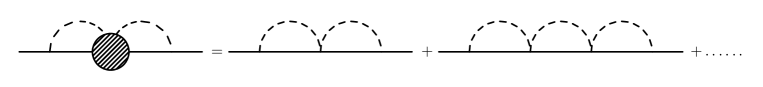
Figure 5: Contribution to the nucleon self-energy.

It is easily verified that $\Sigma$ depends only on $\Gamma^{1/2}$. Using the solution for $\Gamma^{1/2}$ from the previous section in Eq. (25) and integrating over $q_{1}$ and $q_{2}$ we obtain an analytic expression for the contribution of the diagrams in Fig. 5 to the nucleon mass

$$\delta m=-\frac{3\,\stackrel{{\scriptstyle\circ}}{{g_{A}}}^{2}}{4\,F^{2}}\,\frac{N}{D}\,,$$ (27)

where

$$N = \left(m+m_{N}\right)\left(4\,F^{2}-I_{\pi}\right)\biggl{[}\left(m_{N}-m\right)I_{\pi}-\left(m^{2}-M^{2}-2\,m\,m_{N}+m_{N}^{2}\right)\left(m+m_{N}\right)I_{N\pi}\biggr{]}^{2}\,,$$

$$D = 2\,m_{N}\Biggl{\{}8\,m_{N}\,F^{4}+4\,\biggl{[}\left(m-\,m_{N}\right)I_{\pi}+\left(m^{2}-M^{2}-2\,m\,m_{N}+m_{N}^{2}\right)(m+m_{N})\,I_{N\pi}\biggr{]}F^{2}$$ (28)

$$+\,I_{\pi}\biggl{[}\left(m_{N}-m\right)I_{\pi}-\left(m^{2}-M^{2}-2\,m\,m_{N}+m_{N}^{2}\right)\left(m+m_{N}\right)I_{N\pi}\biggr{]}\Biggr{\}}\,.$$

On the other hand, by expanding Eq. (27) in powers of $1/F^{2}$ we can identify the contributions of each diagram separately. Using the IR renormalization scheme and substituting $m=882.8$ MeV Fuchs:2003kq , $m_{N}=938.3$ MeV, $F=92.4$ MeV, $\stackrel{{\scriptstyle\circ}}{{g_{A}}}=1.267$ and $M=139.6$ MeV we obtain

$$\delta m=-0.00233530\,{\rm MeV}=\left(-0.00230219-0.00003305-0.00000007+\cdots\right)\,{\rm MeV}\,.$$ (29)

As can be seen from Eq. (29) the first term in the perturbative expansion reproduces the non-perturbative result well and the higher-order corrections are clearly suppressed.

It is relevant for the chiral extrapolation of lattice data to consider the nucleon mass for larger values of the quark masses. Therefore in Fig. 6 we plot $\delta m$ of Eq. (28) together with the leading contribution (first diagram in Fig. 5) and the leading non-analytic correction to the nucleon mass $\delta m_{3}=-3\,g_{A}^{2}\,M^{3}/(32\,\pi\,F^{2})$ Gasser:1988rb as functions of $M$. As can be seen from this figure, up to $M\sim 500$ MeV the non-perturbative sum of higher-order corrections is suppressed in comparison with the $\delta m_{3}$ term. Also, the leading higher order contribution reproduces the non-perturbative result quite well. On the other hand for $M\gtrsim 600$ MeV the higher-order contributions are no longer suppressed in comparison with $\delta m_{3}$.

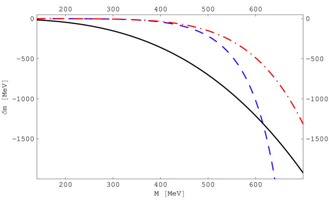
Figure 6: Contributions to the nucleon mass as functions of $M$. The solid, dashed, and dashed-dotted lines correspond to $\delta m_{3}$, $\delta m$, and the contribution of the two-loop diagram in Fig. 5, respectively.

IV Summary and discussion

In this work we have addressed the issue of convergence of perturbative calculations in BChPT by analyzing pion-nucleon scattering and the nucleon mass. By solving the equation for the $\pi N$ vertex function using dimensional regularization we have obtained an exact expression for a sum of an infinite number of loop diagrams. The solution is given in a closed form in terms of one-loop integrals. We have renormalized the obtained non-perturbative expression by applying infrared renormalization Becher:1999he . We compared the perturbative contributions with the re-summed expression for elastic $\pi N$ scattering. We find that already for $s\sim m_{\Delta}^{2}$ the perturbative results approximate the re-summed non-perturbative expression very poorly. As the potential, which has been iterated by solving the equation does not receive contributions from the intermediate $\Delta$ state, we conclude that the inclusion of the $\Delta$ as an explicit degree of freedom does not solve the problem of convergence of the considered loop contributions. In our opinion, to solve this problem one needs to include the $\Delta$ degrees of freedom Hacker:2005fh and simultaneously consider the $\pi N$ scattering equations.

Next, using the non-perturbative result for the $\pi N$ scattering amplitude we have obtained an exact expression corresponding to a sum of an infinite number of diagrams contributing to the nucleon self-energy. Using the infrared renormalization scheme and comparing the non-perturbative contribution to the nucleon mass with contributions of the first several terms in its perturbative expansion we conclude that the so obtained perturbative series for the nucleon mass converges very well. We also considered the correction to the nucleon mass for larger values of quark masses and found that the re-summed higher order contributions become larger than the leading non-analytic contribution for $M\gtrsim 600$ MeV. From this we conclude that for such values of $M$ BChPT cannot be trusted in extrapolations of lattice data. Even if there are large cancelations these cannot be treated systematically in standard BChPT. As we have summed up only a subset of higher-order diagrams, our analysis is not complete and therefore our result should be considered as an estimate for an upper limit of the radius of convergence.

V appendix

One-loop integrals:

$$I^{\mu}_{N\pi}(-p,0) = p^{\mu}\,I^{(p)}_{N\pi}(-p,0)=i\int\frac{d^{n}k}{(2\pi)^{n}}\frac{k^{\mu}}{[(k-p)^{2}-m^{2}+i0^{+}][k^{2}-M^{2}+i0^{+}]}$$

$$= \frac{p^{\mu}}{2p^{2}}\left[(p^{2}-m^{2}+M^{2})\,I_{N\pi}(-p,0)+I_{N}-I_{\pi}\right]\,,$$

$$I_{\pi} = i\,\int\frac{d^{n}k}{(2\pi)^{n}}\frac{1}{k^{2}-M^{2}+i0^{+}}=2\,M^{2}\bar{\lambda}+\frac{M^{2}}{8\pi^{2}}\ln\left(\frac{M}{m}\right)\,,$$

$$I_{N} = i\int\frac{d^{n}k}{(2\pi)^{n}}\frac{1}{k^{2}-m^{2}+i0^{+}}=2\,m^{2}\,\bar{\lambda}\,,$$

$$I_{N\pi}(-p,0) = i\int\frac{d^{n}k}{(2\pi)^{n}}\frac{1}{[(k-p)^{2}-m^{2}+i0^{+}][k^{2}-M^{2}+i0^{+}]}$$ (30)

$$= 2\,\bar{\lambda}+\frac{1}{16\pi^{2}}\left[-1+\frac{p^{2}-m^{2}+M^{2}}{p^{2}}\ln\left(\frac{M}{m}\right)+\frac{2mM}{p^{2}}F(\Omega)\right],$$

where

$$\bar{\lambda} = {m^{n-4}\over(4\pi)^{2}}\left\{{1\over n-4}-{1\over 2}\left[\ln(4\pi)+\Gamma^{\prime}(1)+1\right]\right\}\,,$$

$$F(\Omega) = \left\{\begin{array}[]{ll}\sqrt{1-\Omega^{2}}\arccos(-\Omega),&-1\leq\Omega\leq 1,\\ \sqrt{\Omega^{2}-1}\ln\left(\Omega+\sqrt{\Omega^{2}-1}\right)-i\pi\sqrt{\Omega^{2}-1},&1\leq\Omega,\end{array}\right.\,,$$

$$\Omega = \frac{p^{2}-m^{2}-M^{2}}{2\,m\,M}\,.$$

Infrared renormalized expression for $I_{N\pi}(-p,0)$:

$$I^{IR}_{N\pi}(-p,0) = \frac{1}{16\pi^{2}}\,\frac{p^{2}-m^{2}+M^{2}}{2\,p^{2}}\,\left[2\,\ln\left(\frac{M}{m}\right)-1\right]+F_{IR}(\Omega),$$ (32)

where

$$F_{IR}(\Omega) = \left\{\begin{array}[]{ll}\frac{1}{8\pi^{2}}\,\frac{m\,M}{p^{2}}\,\sqrt{1-\Omega^{2}}\,\arccos\left(-\frac{\alpha+\Omega}{\sqrt{1+2\,\alpha\,\Omega+\alpha^{2}}}\right),&-1\leq\Omega\leq 1,\\ -\frac{1}{16\,\pi^{2}}\ \frac{m\,M}{p^{2}}\,\sqrt{\Omega^{2}-1}\ \ln\,\frac{\alpha+\Omega-\sqrt{\Omega^{2}-1}}{\alpha+\Omega+\sqrt{\Omega^{2}-1}}-\frac{i}{8\,\pi}\ \frac{m\,M}{p^{2}}\,\sqrt{\Omega^{2}-1}\,,&1\leq\Omega,\end{array}\right.$$

and $\alpha=\frac{M}{m}$ .

$$I_{N\pi}=I_{N\pi}(-p,0)|_{p^{2}=m_{N}^{2}}\,.$$ (34)

References

• (1) S. Weinberg, Physica A 96, 327 (1979).
• (2) J. Gasser and H. Leutwyler, Ann. Phys. (N.Y.) 158, 142 (1984).
• (3) J. Gasser and H. Leutwyler, Nucl. Phys. B250, 465 (1985).
• (4) G. Colangelo, J. Gasser, and H. Leutwyler, Phys. Lett. B 488, 261 (2000).
• (5) G. Colangelo, J. Gasser, and H. Leutwyler, Nucl. Phys. B603, 125 (2001).
• (6) I. Caprini, G. Colangelo, J. Gasser, and H. Leutwyler, Phys. Rev. D 68, 074006 (2003).
• (7) I. Caprini, G. Colangelo, and H. Leutwyler, arXiv:hep-ph/0509266.
• (8) I. Caprini, G. Colangelo, and H. Leutwyler, arXiv:hep-ph/0512364.
• (9) G. Colangelo, AIP Conf. Proc.  756, 60 (2005).
• (10) S. Scherer, arXiv:hep-ph/0512291.
• (11) J. Bijnens, arXiv:hep-ph/0604043.
• (12) J. Gasser, M. E. Sainio, and A. Švarc, Nucl. Phys. B307, 779 (1988).
• (13) S. Scherer, in Advances in Nuclear Physics, Vol. 27, edited by J. W. Negele and E. W. Vogt (Kluwer Academic/Plenum Publishers, New York, 2003).
• (14) S. R. Beane, Nucl. Phys. B695, 192 (2004).
• (15) M. Procura, T. R. Hemmert, and W. Weise, Phys. Rev. D 69, 034505 (2004).
• (16) D. B. Leinweber, A. W. Thomas, and R. D. Young, PoS LAT2005, 048 (2005).
• (17) M. Procura, B. U. Musch, T. Wollenweber, T. R. Hemmert, and W. Weise, arXiv:hep-lat/0603001.
• (18) M. F. Lutz and E. E. Kolomeitsev, Nucl. Phys. A700, 193 (2002).
• (19) T. Becher and H. Leutwyler, Eur. Phys. J. C 9, 643 (1999).
• (20) M. R. Schindler, J. Gegelia, and S. Scherer, Phys. Lett. B 586, 258 (2004).
• (21) T. Fuchs, J. Gegelia, and S. Scherer, Eur. Phys. J. A 19, 35 (2004).
• (22) C. Hacker, N. Wies, J. Gegelia, and S. Scherer, Phys. Rev. C 72, 055203 (2005).