Little Higgs model effects at $\gamma\gamma$ collider

Abstract

Though the predictions of the Standard Model (SM) are in excellent agreement with experiments there are still several theoretical problems, such as fine-tuning and the hierarchy problem. These problems are associated with the Higgs sector of the SM, where it is widely believed that some “new physics” will take over at the TeV scale. One beyond the SM theory which resolves these problems is the Little Higgs (LH) model. In this work we shall investigate the effects of the LH model on $\gamma\gamma\to\gamma\gamma$ scattering; where the process $\gamma\gamma\to\gamma\gamma$ at high energies occurs in the SM through diagrams involving $W$, charged quark and lepton loops (and is, therefore, particularly sensitive to any new physics).

I Introduction

It has been known for some time that the $\gamma\gamma\to\gamma\gamma$ scattering amplitude at high energies will be a very useful tool in the search for new particles and interactions in an $e^{+}e^{-}$ linear collider operated in the $\gamma\gamma$ mode. In particular, as according to present ideas, this scattering can be achieved by colliding $e^{\pm}$ beams at a future linear collider, such as the ILC, with laser photons (which are subsequently backscattered, through the Compton effect) to produce very energetic photons of high luminosity along the $e^{\pm}$ direction; while the $e^{\pm}$ beams would loose most of their energy. As such, these searches may involve either the direct production of new degrees of freedom (for example, charginos, light sleptons or a light stop in SUSY models); or the precise study of the production of SM particles, where the the new degrees of freedom contribute virtually in some loop diagrams. In this respect, processes like $\gamma\gamma\to\gamma\gamma$, $\gamma\gamma\to Z\gamma$, $\gamma\gamma\to ZZ$ should all provide very important tools for searching or constraining new physics Choudhury:1999gp ; particularly as the SM contributions in these processes first appear at the one-loop level and should be small.

As a large number of helicity amplitudes can contribute to these processes, due to the presence of spin-one particles in the initial and final states, considerations of symmetries and other invariances is required to reduce this number. Furthermore, in the SM the amplitudes of $\gamma\gamma\to\gamma\gamma$ will have contributions from one-loop diagrams mediated by charged fermions (leptons and quarks) and $W$-bosons. At large energies ($\sqrt{s_{\gamma\gamma}}\geq 250GeV$) it is know that the $W$ contributions dominate over the fermionic contributions. At these energies it should also be noted that the dominant amplitudes are predominantly imaginary. Therefore we expect that any new physics effects in the $\gamma\gamma\to\gamma\gamma$ process may come from the interference terms between the predominantly imaginary SM amplitudes and new physics effects to these amplitudes.

At this point we would like to point out that though the SM has been very successful in explaining all electroweak interactions probed so far, there is no symmetry or relation which protects the mass of the Higgs boson. In fact the Higgs mass diverges quadratically when quantum corrections in the SM are taken into account. But precision electroweak data demands the lightest Higgs boson mass be $\sim 200$GeV! In order for this to happen we either need to invoke some symmetries which will protect the Higgs mass to a much higher scale (possibly GUT scale) or assume that the SM is an effective theory valid up to only the electroweak scale. In either of these possibilities it is expected that some new physics should takeover from the SM at the TeV scale. As such, Supersymmetry has provided one popular example of new physics, where additional symmetries are invoked which help protect the Higgs mass up to GUT scale. Recently a new approach to address this problem has been advocated, the approach popularly known as the “Little Higgs models”, which addresses some of the problems in the SM by making the Higgs boson a pseudo-Goldstone boson of a symmetry which is broken at some higher scale $\Lambda$. The suggestion of making the Higgs a pseudo-Goldstone boson was proposed some time ago Georgi:1975tz but has been revived recently, where such models have been successfully constructed by Arkani-Hamed, Cohen and Georgi Arkani-Hamed:2001nc . The successful Little Higgs models are constructed in such a way that no single interaction breaks all the symmetries, but the symmetries are broken collectively. In these models the scale $\Lambda$ ($=4\pi f$) is chosen to be $\sim 10$TeV. The scale $\Lambda$ acts as a cut-off which separates the weakly interacting low energy range from possible strongly interacting sectors at higher energies. The Higgs fields then acquire a mass radiatively at the electroweak scale. Note that in this model the Higgs field remains light, being protected by the approximate global symmetry and free from any one-loop quadratic sensitivity to the cutoff scale $\Lambda$. Note also, that in doing this we are required to introduce several new heavy gauge bosons and other new particles, which shall be discussed further in section 2.

However, it must be noted that the originally proposed implementations of the LH approach suffered from severe constraints from precision electroweak measurements Yue:2004xt , which could only be satisfied by finely tuning the model parameters. The most serious constraint resulted from the tree-level corrections to precision electroweak observables due to the exchanges of the additional heavy gauge bosons present in the theories (because their masses are much smaller than the cut-off scale), as well as from the small but non-vanishing vev of an additional weak-triplet scalar field. As a result, masses of new particles had to be raised, and the fine-tuning of the Higgs boson mass is re-introduced. Motivated by these constraints, several new variants of the LH model were proposed Chang:2003un . Particularly interesting is the implementation of the $Z_{2}$ symmetry, called T-parity, into the model, as proposed in references Cheng:2005as . T-parity explicitly forbids any tree-level contribution from the new heavy gauge bosons to the observables involving only SM particles as external states. It also forbids the interactions that induced the triplet vev. As a result, in T-parity symmetric LH models, corrections to precision electroweak observables are generated exclusively at loop level. This implies that the constraints are generically weaker than in the tree-level case, and fine tuning can be avoided Hubisz:2005tx .

Note that due to T-parity the lightest T-odd particle becomes stable and a good candidate for dark matter. This is an interesting feature of the model, because the existence of dark matter is now established by recent cosmological observations Asano:2006nr . Since the lightest T-odd particle is electrically and colour neutral, and has a mass of ${\cal O}(100)$GeV Cheng:2005as ; Asano:2006nr in many LH models with T-parity, these models provide a WIMP dark matter candidate Cheng:2005as , and are able to account for the large scale structure of the present universe.

With this in mind, we review the LH model we have used in section 2 before proceeding to investigate the helicity amplitudes of the scattering process $\gamma\gamma\to\gamma\gamma$ in section 3. Finally we conclude with the discussion of the results of our numerical analysis in section 4.

II Little Higgs models

In this section we will briefly describe the LH models which we have used in our analysis. In particular the minimal version of the LH model, the so-called Littlest Higgs model Han:2003wu .

To begin, let us recall that it is known that the scalar mass in a generic quantum field theory will receive quadratically divergent radiative corrections, all the way up to the cut-off scale. The LH model solves this problem by eliminating the lowest order contributions via the presence of a partially broken global symmetry (where the non-linear transformation of the Higgs fields under this global symmetry prohibits the existence of a Higgs mass term of the form $m^{2}|h|^{2}$). This is done by introducing a new set of heavy gauge bosons (with the same quantum numbers as the SM gauge bosons), where the gauge couplings to the Higgs bosons are patterned in such a way that the quadratic divergences induced in the SM gauge boson loops are canceled by the quadratic divergence induced by the heavy gauge bosons at one-loop level. One also introduces a heavy fermionic state which couples to the Higgs field in a specific way, so that the one-loop quadratic divergence induced by the top-quark Yukawa coupling to the Higgs boson is canceled. Furthermore, extra Higgs fields exist as the Goldstone boson multiplets from the global symmetry breaking. On this framework the Littlest Higgs model was introduced, which was based on an $SU(5)/SO(5)$ coset. The phenomenology of this model was discussed in great detail in precision tests Han:2003wu ; Yue:2004xt and low energy measurements Buras:2004kq . LH models generically also predict the existence of a doubly charged triplet Higgs. The phenomenology of triplet Higgs within the context of the LH model has also been extensively studied in the literature Han:2005nk . A detailed review of LH models can be found in Schmaltz:2005ky .

The model we shall use in our analysis, the Littlest Higgs model Han:2003wu ; Schmaltz:2005ky , is a non-linear $\sigma$ model based on an $SU(5)$ global symmetry which contains a gauged $\left[SU(2)\times U(1)\right]_{1}\bigotimes\left[SU(2)\times U(1)\right]_{2}$ symmetry with couplings $g_{1},g_{2},g_{1}^{\prime}$ and $g_{2}^{\prime}$ as its subgroup. Furthermore, the global $SU(5)$ symmetry is broken into $SO(5)$ by the vacuum expectation value of the sigma field

$$\Sigma_{0}=\left(\begin{array}[]{ccc}0&0&\leavevmode\hbox{\small 1\normalsize\kern-3.30002pt1}\\ 0&1&0\\ \leavevmode\hbox{\small 1\normalsize\kern-3.30002pt1}&0&0\end{array}\right).$$ (II.1)

Where 11 is the $2\times 2$ identity matrix. This breaking simultaneously breaks the gauge group to an $SU(2)\times U(1)$ subgroup, which is identified with the SM group. The breaking of the global $SU(5)\to SO(5)$ gives rise to 14 goldstone bosons, $\Pi=\pi^{a}X^{a}$ which can be written as

$$\Sigma=\displaystyle e^{i\Pi/f}\Sigma_{0}e^{i\Pi^{T}/f}=\Sigma_{0}+\frac{2i}{f}\Pi\Sigma_{0}+{\cal O}(1/f^{2}),$$ (II.2)

where $X^{a}$ corresponds to the broken $SU(5)$ generators. Four of the fourteen Goldstone bosons are absorbed by the broken gauge generators, and the remaining ten Goldstones are parameterized as:

$$\Pi=\left(\begin{array}[]{ccc}&h^{\dagger}/\sqrt{2}&\Phi^{\dagger}\\ h/\sqrt{2}&&h^{*}/\sqrt{2}\\ \Phi&h^{T}/\sqrt{2}&\end{array}\right),$$ (II.3)

where $h$ is the SM Higgs doublet and $\Phi$ is a complex $SU(2)$ triplet:

$$\Phi=\left(\begin{array}[]{cc}\Phi^{++}&\Phi^{+}/\sqrt{2}\\ \Phi^{+}/\sqrt{2}&\Phi^{0}\end{array}\right).$$ (II.4)

The kinetic term for the $\Sigma$ field can be written as

$${\cal L}_{kin}=\displaystyle\frac{f^{2}}{8}\mathrm{Tr}\left\{D_{\mu}\Sigma(D^{\mu}\Sigma)^{\dagger}\right\},$$ (II.5)

where

$$D_{\mu}\Sigma=\partial_{\mu}\Sigma-i\Sigma_{j}\left[g_{j}W_{j}^{a}(Q_{j}^{a}\Sigma+\Sigma Q_{j}^{aT})+g^{\prime}_{j}B_{j}(Y_{j}\Sigma+\Sigma Y_{j})\right].$$ (II.6)

In the above $j=1,2$, the $Q_{j}$ and $Y_{j}$ are the gauged generators, $B_{j}$ and $W_{j}^{a}$ are the $U(1)_{j}$ and $SU(2)_{j}$ gauge fields, respectively, and $g_{j}$ and $g^{\prime}_{j}$ are the corresponding coupling constants.

As stated earlier, the vev ($\Sigma_{0}$) given in eqn(II.1) breaks the gauge group to the diagonal one, which is then identified with the SM group. This generates mass and mixings of the gauge bosons. The heavy gauge boson mass eigenstates are given by

$$W_{H}^{a}=-cW_{1}^{a}+sW_{2}^{a}~{}~{},~{}~{}B_{H}=-c^{\prime}B_{1}+s^{\prime}B_{2},$$ (II.7)

where $s,s^{\prime},c$ and $c^{\prime}$ are the mixing angles given by

$$c^{\prime}= g^{\prime}/g_{2}^{\prime}~{}~{}~{},~{}~{}~{}s^{\prime} =g^{\prime}/g_{1}^{\prime},$$

$$c= g/g_{2}~{}~{}~{},~{}~{}~{}s =g/g_{1}.$$ (II.8)

These couplings can be related to the SM couplings ($g,g^{\prime}$) by Han:2003wu :

$$\frac{1}{g^{2}}=\frac{1}{g_{1}^{2}}+\frac{1}{g_{2}^{2}}~{}~{}~{},~{}~{}~{}\frac{1}{g^{\prime 2}}=\frac{1}{g_{1}^{\prime 2}}+\frac{1}{g_{2}^{\prime 2}},$$ (II.9)

where the masses of heavy gauge bosons will then be:

$$M_{W_{H}}^{2}=\frac{f^{2}}{4}\left(g_{1}^{2}+g_{2}^{2}\right)~{}~{},~{}~{}M_{B_{H}}^{2}=\frac{f^{2}}{20}\left(g_{1}^{\prime 2}+g_{2}^{\prime 2}\right).$$ (II.10)

The orthogonal combination of these gauge bosons are identified with the SM $W$ and $B$.

In the SM the top quark introduces quadratic corrections to the Higgs boson mass. The LH model addresses this problem by the introduction of a new set of heavy fermions which couple to the Higgs such that it cancels the quadratic divergences to the Higgs mass; due to the SM top quark. A vector like top quark is usually introduced in the LH model to do this job. The Yukawa interactions in the LH model are chosen to be:

$${\cal L}_{Y}={1\over 2}\lambda_{1}f\epsilon_{ijk}\epsilon_{xy}\chi_{i}\Sigma_{jx}\Sigma_{ky}u_{3}^{\prime c}+\lambda_{2}f\tilde{t}\tilde{t}^{\prime c}+h.c.$$ (II.11)

with $i,j,k$ summed over 1, 2, 3 and $x$, $y$ summed over 4, 5. $\chi_{i}=(b_{3},t_{3},\tilde{t})$, $b_{3}$ and $t_{3}$ are the SM bottom and top quarks, $(\tilde{t},\tilde{t}^{\prime c})$ is the new vector like top quark and $u_{3}^{\prime c}$ is the SM right handed top quark.

Expanding the $\Sigma$ field and diagonalizing the mass matrix we arrive at the physical states:

$$m_{t}\sim\frac{v\lambda_{1}\lambda_{2}}{\sqrt{\lambda_{1}^{2}+\lambda_{2}^{2}}}~{}~{}~{}~{},~{}~{}~{}~{}m_{T}\sim f\sqrt{\lambda_{1}^{2}+\lambda_{2}^{2}}.$$ (II.12)

These masses are parameterized in term of $x_{L}$, defined as:

$$x_{L}=\frac{\lambda_{1}^{2}}{\lambda_{1}^{2}+\lambda_{2}^{2}}.$$ (II.13)

In the LH models there is no Higgs potential at tree level, this is generated at one-loop level via the interactions with gauge bosons and fermions. This is similar to a Coleman-Weinberg type of potential. This gives the Higgs masses as:

$$M_{\Phi}^{2}=2m_{H}^{2}\frac{f^{2}}{v^{2}}\frac{1}{1-\left(\frac{4v^{\prime}f}{v^{2}}\right)},$$ (II.14)

where $m_{H}$ is the SM Higgs boson mass. Therefore, for this kind of LH model (based on $SU(5)/SO(5)$) we have five input parameters, in addition to the SM Higgs mass, explicitly, these are

$$s,s^{\prime},x_{L},f,v^{\prime}.$$

The advantage of this model now becomes apparent; by noting that as the gauge generators are embedded in the $SU(5)$ group, in such a way as to commute with an $SU(3)$ subgroup, one pair of gauge couplings must be set to zero. Therefore the Higgs mass would be an exact Goldstone boson and massless. As such, any diagram renormalizing the Higgs mass will vanish unless it involves at least two of the gauge couplings. Note that at the one-loop level all diagrams satisfying this condition are only logarithmically divergent. Therefore the symmetry breaking mechanism protects the Higgs mass from quadratic divergences at this level. Generically the particle spectrum of the LH model, apart from SM particles is:

• Heavy vector like top quark (T);

• Heavy gauge bosons: charged ($W_{H}$), neutral( $Z_{H},A_{H}$);

• Additional triplet Higgs: ($\Phi^{0},\Phi^{+},\Phi^{++}$).

As mentioned in the introduction, the original LH models were severely constrained by precision electroweak experiments Han:2003wu ; Yue:2004xt . The main constraints coming from the $\rho$ parameter and the $Z\to b\bar{b}$ Yue:2004xt vertex contributions. Other models which evade these constraints have been proposed, but all of these enlarge the global or gauge symmetries. Recently Cheng and Low Cheng:2005as introduced a discrete $Z_{2}$ symmetry, which we now call “T-parity” to resolve the electroweak precision constraints in the LH models. The advantages of introducing T-parity is two fold. Firstly it helps relaxing the precision constraints and secondly it also provides a dark matter candidate. The new parity is an exchange of the two gauge groups and the Lagrangian in eqn (II.5) is invariant under this exchange provided that $g_{1}=g_{2}$ and $g^{\prime}_{1}=g^{\prime}_{2}$. The implication of this is that the gauge boson mass eigenstates will have the form $W_{\pm}=\frac{1}{\sqrt{2}}(W_{1}\pm W_{2})$ and $B_{\pm}=\frac{1}{\sqrt{2}}(B_{1}\pm B_{2})$. The SM gauge bosons are even under T-parity and are designated by a $+$ subscript, and the new “T-odd” gauge bosons are designated by a $-$ subscript. The different T-parity states do not mix and after electroweak symmetry breaking, the Weinberg angle is given by the usual SM relation, as are other electroweak observables (thus removing the constraint). Note further that as the transformation law ensures that the complex $SU(2)$ triplet is odd under T-parity, whilst the Higgs doublet is even, the trilinear coupling $H^{\dagger}\phi H$ is forbidden. This further relaxes precision electroweak constraints on the model.

Thus the main implications of the introduction of T-parity are:

• All new particles (except one heavy top quark) are odd under T-parity;

• T-parity exchanges $[SU(2)\times U(1)]_{1}$ and $[SU(2)\times U(1)]_{2}$;

• T-parity imposes a relationship between the couplings, for example $g_{1}=g_{2}$, $g_{1}^{\prime}=g_{2}^{\prime}$;

• The fermion sector is extended to include T-odd fermions;

• There is no vev to the triplet Higgs. This being assured by the absence of a $H\Phi H$ coupling.

In such a model ($SU(5)/SO(5)$ with T-parity) the input model parameters (apart from SM Higgs mass $m_{H}$) are:

$$f~{},~{}~{}\frac{\lambda_{1}}{\lambda_{2}},~{}~{}\kappa.$$

The first two have been defined before and $\kappa$ is a free parameter whose range is $0.5\leq\kappa\leq 1.5$ Hubisz:2005tx . As we are interested in the $\gamma\gamma\to\gamma\gamma$ process, where this process occurs at one-loop by the mediation of charged particles, it should be noted that in the SM this process is mediated by charged $W$ and fermions (charged leptons and quarks). This process in the LH model can also be mediated by charged gauge bosons ($W_{H}$), charged Higgs ($\Phi^{-},\Phi^{--}$) and new fermions ($T$ in the LH model without T-parity; note that in the LH model with T-parity, there shall also be $T_{+},T_{-}$ and heavy T-odd fermions which can mediate the process). To conclude this section, we have given the mass spectrum of these particles in the LH models in Table 1.

Particle	$W_{H}$	$\Phi$	$m_{t}$	$T_{-}$	$T_{+}$	$f_{H}$
Masses (LH with T-parity)	$gf$	$\frac{\sqrt{2}m_{H}f}{v}$	$\frac{\lambda_{1}\lambda_{2}v}{\sqrt{\lambda_{1}^{2}+\lambda_{2}^{2}}}$	$\lambda_{2}f$	$\sqrt{\lambda_{1}^{2}+\lambda_{2}^{2}}f$	$\kappa f$
Masses (LH without T-parity)	$\frac{gf}{2sc}$	$\frac{\sqrt{2}m_{H}f/v}{\sqrt{\left[1-(4v^{\prime}f/v^{2})^{2}\right]}}$	$\frac{\lambda_{1}\lambda_{2}v}{\sqrt{\lambda_{1}^{2}+\lambda_{2}^{2}}}$	-	-	-

Table 1: Mass spectrum of the LH models. $v$ is the vev of the SM Higgs and $m_{H}$ is the SM Higgs mass. In the model without T-parity we have only one vector like top quark with mass $m_{T}=\sqrt{\lambda_{1}^{2}+\lambda_{2}^{2}}f$. $f_{H}$ are the T-odd fermions in the LH with T-parity.

III The $\gamma\gamma\to\gamma\gamma$ crossections

The process

$$\gamma(p_{1},\lambda_{1})\gamma(p_{2},\lambda_{2})\to\gamma(p_{3},\lambda_{3})\gamma(p_{4},\lambda_{4})$$ (III.1)

can be represented by sixteen possible helicity amplitudes $F_{\lambda_{1}\lambda_{2}\lambda_{3}\lambda_{4}}(\hat{s},\hat{t},\hat{u})$, where the $p_{i}$ and $\lambda_{i}$ represent the respective momenta and helicities; the $\hat{s}$, $\hat{t}$ and $\hat{u}$ are the usual Mandelstam variables. By the use of Bose statistics, crossing symmetries and demanding parity and time-invariance, these sixteen possible helicity amplitudes can be expressed in terms of just three amplitudes, namely (the relationship between various helicity amplitudes as given in appendix A)

$$F_{++++}(\hat{s},\hat{t},\hat{u}),\hskip 14.22636ptF_{+++-}(\hat{s},\hat{t},\hat{u}),\hskip 14.22636ptF_{++--}(\hat{s},\hat{t},\hat{u}).$$ (III.2)

As such, the cross-section for this process can be expressed as Jikia:1993tc :

$$\displaystyle\frac{d\sigma}{d\tau d\cos\theta^{*}} = \displaystyle\frac{d\bar{L}_{\gamma\gamma}}{d\tau}\left\{\frac{d\bar{\sigma}_{0}}{d\cos\theta^{*}}+\langle\xi_{2}\xi^{\prime}_{2}\rangle\frac{d\bar{\sigma}_{22}}{d\cos\theta^{*}}+\left[\langle\xi_{3}\rangle\cos 2\phi+\langle\xi^{\prime}_{3}\rangle\cos 2\phi\right]\right.$$ (III.3)

$$\hskip 14.22636pt\times\displaystyle\frac{d\bar{\sigma}_{3}}{d\cos\theta^{*}}+\langle\xi_{3}\xi^{\prime}_{3}\rangle\left[\frac{d\bar{\sigma}_{33}}{d\cos\theta^{*}}\cos 2(\phi+\phi^{\prime})+\frac{d\bar{\sigma}^{\prime}_{33}}{d\cos\theta^{*}}\cos 2(\phi-\phi^{\prime})\right]$$

$$\left.\hskip 14.22636pt\displaystyle+\left[\langle\xi_{2}\xi^{\prime}_{3}\rangle\sin 2\phi^{\prime}-\langle\xi_{3}\xi^{\prime}_{2}\rangle\sin 2\phi^{\prime}\right]\frac{d\bar{\sigma}_{23}}{d\cos\theta^{*}}\right\},$$

where $d\bar{L}_{\gamma\gamma}$ describes the photon-photon luminosity in the $\gamma\gamma$ mode and $\tau=s_{\gamma\gamma}/s_{ee}$. Note that $\xi_{2}$, $\xi^{\prime}_{2}$, $\xi_{3}$ and $\xi^{\prime}_{3}$ are the Stokes parameters. Furthermore Jikia:1993tc ; Gounaris:1999gh ,

$$\frac{d\bar{\sigma}_{0}}{d\cos\theta^{*}} = \left(\frac{1}{128\pi\hat{s}}\right)\sum_{\lambda_{3}\lambda_{4}}\left[\left|F_{++\lambda_{3}\lambda_{4}}\right|^{2}+\left|F_{+-\lambda_{3}\lambda_{4}}\right|^{2}\right],$$

$$\frac{d\bar{\sigma}_{22}}{d\cos\theta^{*}} = \left(\frac{1}{128\pi\hat{s}}\right)\sum_{\lambda_{3}\lambda_{4}}\left[\left|F_{++\lambda_{3}\lambda_{4}}\right|^{2}-\left|F_{+-\lambda_{3}\lambda_{4}}\right|^{2}\right],$$

$$\frac{d\bar{\sigma}_{3}}{d\cos\theta^{*}} = \left(-\frac{1}{64\pi\hat{s}}\right)\sum_{\lambda_{3}\lambda_{4}}\mathrm{Re}\left[F_{++\lambda_{3}\lambda_{4}}F^{*}_{-+\lambda_{3}\lambda_{4}}\right],$$

$$\frac{d\bar{\sigma}_{33}}{d\cos\theta^{*}} = \left(\frac{1}{128\pi\hat{s}}\right)\sum_{\lambda_{3}\lambda_{4}}\mathrm{Re}\left[F_{+-\lambda_{3}\lambda_{4}}F^{*}_{-+\lambda_{3}\lambda_{4}}\right],$$

$$\frac{d\bar{\sigma}^{\prime}_{33}}{d\cos\theta^{*}} = \left(\frac{1}{128\pi\hat{s}}\right)\sum_{\lambda_{3}\lambda_{4}}\mathrm{Re}\left[F_{++\lambda_{3}\lambda_{4}}F^{*}_{--\lambda_{3}\lambda_{4}}\right],$$

$$\frac{d\bar{\sigma}_{23}}{d\cos\theta^{*}} = \left(\frac{1}{64\pi\hat{s}}\right)\sum_{\lambda_{3}\lambda_{4}}\mathrm{Im}\left[F_{++\lambda_{3}\lambda_{4}}F^{*}_{+-\lambda_{3}\lambda_{4}}\right].$$ (III.4)

To obtain the total cross-section from the above expressions the integration over $cos\theta^{*}$ has to be done in the range $0\leq\cos\theta^{*}\leq 1$. However, the whole range of $\theta^{*}$ will not be experimentally observable, hence, for our numerical estimates we will restrict the scattering angle to be $|\cos\theta^{*}|\leq\cos 30^{\circ}$. It should be noted that of the above mentioned cross-sections only $d\bar{\sigma}_{0}/d\cos\theta^{*}$ should be positive, where the angle $\theta^{*}$ is the scattering angle of the photons in $\gamma\gamma$ rest frame. The process $\gamma\gamma\to\gamma\gamma$ proceeds through the mediation of charged particles. In the SM these charged particles were charged gauge bosons ($W$), quarks and charged leptons. In the LH model, in addition to the charged gauge bosons and fermions, we also have charged scalars. The analytical expressions of the contributions from fermions, gauge bosons and scalars to the helicity amplitudes are given in Jikia:1993tc and are quoted in Appendix A. With these equations in hand we shall, in the next section, analyse what effects the LH models will have on these cross-sections.

IV Results and Conclusions

In this section we shall present our numerical analysis of the $\gamma\gamma\to\gamma\gamma$ scattering in the LH model, with and without T-parity. Note that in the $\gamma\gamma$ scattering process the helicity amplitudes are proportional to the fourth power of the charge of the particle circulating in the box i.e.

$$F_{\lambda_{1}\lambda_{2}\lambda_{3}\lambda_{4}}\propto Q^{4},$$

where $Q$ is the charge of the particle. In the LH models we generically have a triplet of scalar particles one of which is doubly charged, such as $\Phi^{--}$. This results in a factor of 16 in the amplitude and hence a factor of 256 in the cross-section. This should provide noticeable signatures in the cross-sections.

In our first set of results, presented in figures (1,2), we have shown the contribution of LH particles to the various helicity amplitudes introduced earlier. In figure (1) we have shown the behavior of both real and imaginary parts of the helicity amplitudes for $\theta^{*}=90^{\circ}$ and in figure (2) the results have been plotted for $\theta^{*}=30^{\circ}$. Note that for a scattering angle ($\theta^{*}$) of $90^{\circ}$ we have $\hat{u}=\hat{t}$, which results in $F_{+--+}=F_{+-+-}$. Whereas this relationship is not present for other values of the scattering angle.

We should note, at this point, that the $\gamma\gamma\to\gamma\gamma$ scattering proceeds through loops, both in the SM and in the LH models. In these loops intermediate particles are pair produced (which is why LH models with T-parity are particularly interesting as precision and cosmological constraints on LH particle masses is much weaker Asano:2006nr ; Hubisz:2005tx ). In the SM these are dominated by $W$ loops, leading to a peak in the SM cross-sections around the threshold of the $W$ pair production Gounaris:1999gh . Similarly, in the LH model (with and without T-parity), the dominant contribution will come from the new heavy $W$-boson and the Higgs particles (especially those that are doubly charged), once we exceed the threshold for the pair production of these particles. As such, we have plotted the various cross-sections for a range of energies ($\sqrt{s_{\gamma\gamma}}$) well above the threshold for the SM $W$-bosons, but in the vicinity of the pair production energy for the new particles in the LH models, see figures (3,4). Note further, that we have integrated our differential cross-sections in the angular range $30^{\circ}\leq\theta^{*}\leq 150^{\circ}$.

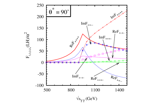
Figure 1: Helicity amplitudes of the LH (with T-parity) contributions for $\theta^{*}=90^{\circ}$. For this plot we have taken $f=700$ GeV. For $\theta^{*}=90^{\circ}$ we have $F_{+--+}=F_{+-+-}$.

We have plotted the SM value and LH value of the various cross-sections introduced in the previous section in figures (3,4). As expected the deviation in the SM value of the cross-sections becomes visible around the threshold of the pair production of LH particles. At present there are very stringent constraints on the masses of LH particles in models without T-parity Yue:2004xt ; Han:2003wu ; Buras:2004kq , as can be seen from figure (3), the deviation from SM values occurs at a very high value of $\sqrt{s_{\gamma\gamma}}$. However, as has noted earlier, in LH models with T-parity a comparatively lower value of the LH particle masses is allowed, which is reflected in the plots in figure (4).

For $\gamma\gamma\to\gamma\gamma$ scattering the LH particles which contribute are the charged gauge bosons ($W_{H}$), charged Higgs and charged fermions. The present constraints on the LH models without T-parity forces the masses of all the new heavy particles to be of the order of TeV. As we are only concerned with charged particles the only parameters of interest in the LH model without T-parity we will be $f$, $x_{L}$, $s$ (as defined earlier in section 2). The plots for LH model with T-parity are shown in figure (4), where we have chosen $\lambda_{1}/\lambda_{2}$ to be 1.

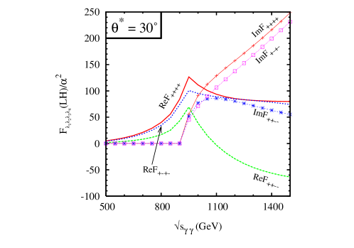
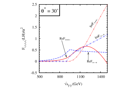
Figure 2: Helicity amplitudes of LH (with T-parity) contributions for $\theta^{*}=30^{\circ}$.

In all cases we can get substantial deviations in the cross-sections due to LH effects, these effects being prominent for relatively lower values of $\sqrt{s_{\gamma\gamma}}$ for the models with T-parity, where we have weaker constraints on the model parameters. It should be noted that the $\sigma_{3}$ and $\sigma^{\prime}_{33}$ provide the most interesting results, where the $\sigma_{3}$ is the only cross-section with pronounced “dips” (these being more pronounced when T-parity is included in the model). The location of these “dips” being dependent on the model parameters. The other feature of note in these plots are the pronounced peaks in the $\sigma^{\prime}_{33}$ cross-section. The LH model effects are more pronounced in $\sigma_{3}$ and $\sigma^{\prime}_{33}$. The SM values of the cross-sections $\sigma_{3}$ and $\sigma^{\prime}_{33}$ are relatively small as compared to the other cross-sections, however, the new physics (the LH model here) effects in these two cross-sections are very striking. These effects mainly depend upon the LH parameter $f$ (the symmetry breaking scale of the global symmetry). In LH models without T-parity the allowed value of $f$ is high, hence the masses of the new heavy particles are high. This results in the deviations, in LH results from SM results, as manifesting at higher values of the invariant mass. Whereas, in the case of T-parity models a much lower value of $f$ is allowed. This now results in lower mass values of T-odd particles; resulting in the onset of LH deviations at a much lower invariant mass.

The results which we have presented for the process $\gamma\gamma\to\gamma\gamma$ are rather generic and can be used as a probe for heavy charged gauge bosons and charged scalars. In our results we have tried to focus ourselves to the range of cm energy ($\sqrt{s_{\gamma\gamma}}$) which is close to the threshold of the pair production of the particles. The deviations from SM results as shown in figures (3,4) will not be observable in the proposed International Linear Collider (ILC), but will be easily probed in a multi-TeV $e^{+}e^{-}$ Compact linear collider (CLIC); where it is proposed to build an $e^{+}e^{-}$ linear collider with a center of mass energy from 0.5 - 3TeV. Generically such a mode should lead to $\gamma\gamma$ collisions at cm energies $E^{\gamma\gamma}_{cm}\leq 0.8E^{ee}_{cm}$. Furthermore, the polarized cross-sections $\sigma_{3}$ and $\sigma^{\prime}_{33}$ can be used to test the spin structure of the particle loops which are responsible for the $\gamma\gamma\to\gamma\gamma$ process Gounaris:1999gh . In summary the $\gamma\gamma\to\gamma\gamma$ process is a very clean process which shall provide a very useful tool for testing LH type models.

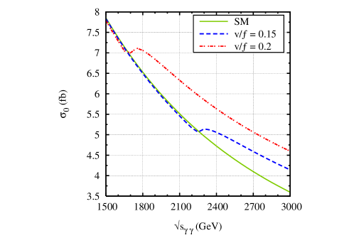
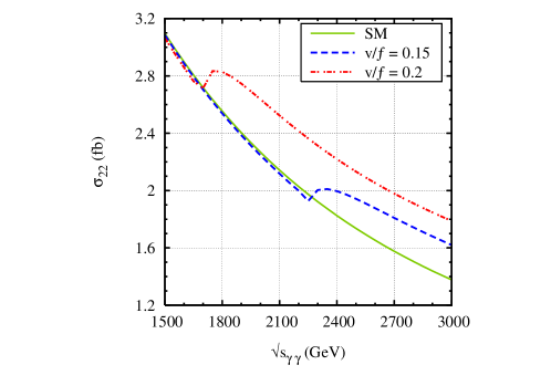
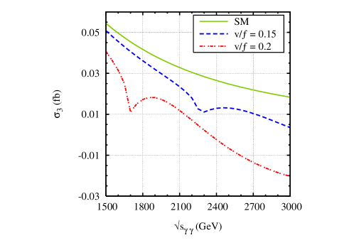
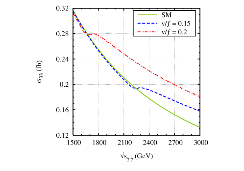
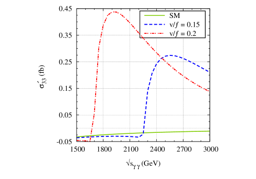
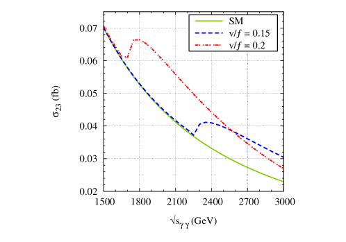
Figure 3: Results for the cross-sections integrated in the range $30\leq\theta^{*}\leq 150$ for various values of $v/f$. Other LH model parameters are: $x_{L}=0.2,s=s^{\prime}=0.6$.

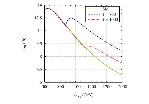
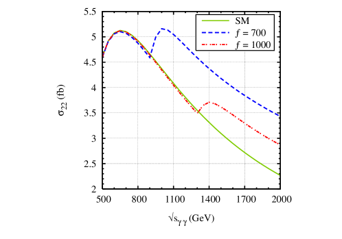
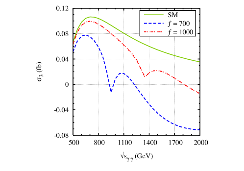
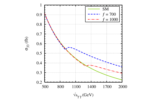
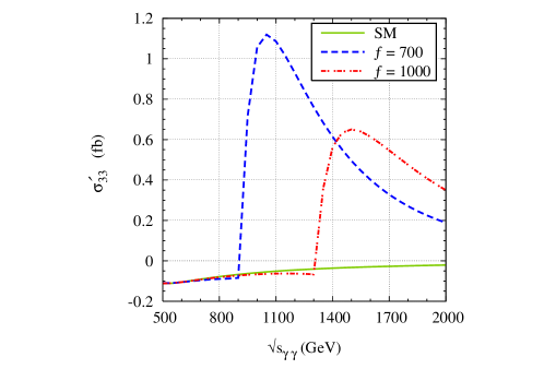
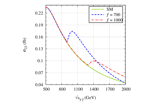
Figure 4: Results for the cross-sections integrated in the range $30\leq\theta^{*}\leq 150$ for various values of $f$ (in GeV) in the LH model with T-parity.

Appendix A Helicity amplitudes

As noted earlier in this paper, for the process;

$$\gamma(p_{1},\lambda_{1})\gamma(p_{2},\lambda_{2})\to\gamma(p_{3},\lambda_{3})\gamma(p_{4},\lambda_{4}),$$ (A.1)

the helicity amplitudes can be denoted $F_{\lambda_{1}\lambda_{2}\lambda_{3}\lambda_{4}}(\hat{s},\hat{t},\hat{u})$, where the momenta and helicities of the incoming and outgoing photons are as denoted in the above equation, and where we have used the Mandelstam variables $\hat{s}=(p_{1}+p_{2})^{2}$, $\hat{t}=(p_{1}-p_{3})^{2}$ and $\hat{u}=(p_{1}-p_{4})^{2}$. Recall that the use of Bose statistics, crossing symmetry, and parity and time inversion invariance results in the 16 possible helicity amplitudes as being expressible in terms of just three amplitudes. Namely, $F_{+++-}(\hat{s},\hat{t},\hat{u})$, $F_{++--}(\hat{s},\hat{t},\hat{u})$ and $F_{++++}(\hat{s},\hat{t},\hat{u})$ through Jikia:1993tc .

$$F_{\pm\pm\mp\pm}(\hat{s},\hat{t},\hat{u}) = F_{\pm\mp\pm\pm}(\hat{s},\hat{t},\hat{u})=F_{\pm\mp\mp\mp}(\hat{s},\hat{t},\hat{u})=F_{---+}(\hat{s},\hat{t},\hat{u})$$ (A.2)

$$= F_{+++-}(\hat{s},\hat{t},\hat{u}),$$

$$F_{--++}(\hat{s},\hat{t},\hat{u}) = F_{++--}(\hat{s},\hat{t},\hat{u}),$$ (A.3)

$$F_{\pm\mp\pm\mp}(\hat{s},\hat{t},\hat{u}) = F_{----}(\hat{u},\hat{t},\hat{s})=F_{++++}(\hat{u},\hat{t},\hat{s}),$$ (A.4)

$$F_{\pm\mp\mp\pm}(\hat{s},\hat{t},\hat{u}) = F_{\pm\mp\pm\mp}(\hat{s},\hat{u},\hat{t})=F_{++++}(t,s,u)=F_{++++}(\hat{t},\hat{u},\hat{s}).$$ (A.5)

Note that in expressing the SM and LH helicity amplitudes we shall use the notation of B, C and D functions as given in Hagiwara:1994pw . The $B_{0}$, $C_{0}$ and $D_{0}$ are the usual one-loop functions first introduced by Passarino and Veltman Passarino:1978jh . The charged gauge boson contributions to the helicity amplitudes can be written as Jikia:1993tc :

$$\displaystyle\frac{F_{++++}^{W}(\hat{s},\hat{t},\hat{u})}{\alpha^{2}} = 12-12\left(1+\displaystyle\frac{2\hat{u}}{\hat{s}}\right)B_{0}(\hat{u})-12\left(1+\frac{2\hat{t}}{\hat{s}}\right)B_{0}(\hat{t})$$ (A.6)

$$\displaystyle\hskip 5.69046pt+\frac{24m_{W}^{2}\hat{t}\hat{u}}{\hat{s}}D_{0}(\hat{u},\hat{t})+16\left(1-\frac{3m_{W}^{2}}{2\hat{s}}-\frac{3\hat{t}\hat{u}}{4\hat{s}^{2}}\right)$$

$$\times\displaystyle\left[2\hat{t}C_{0}(\hat{t})+2\hat{u}C_{0}(\hat{u})-\hat{t}\hat{u}D_{0}(\hat{t},\hat{u})\right]+8\left(\hat{s}-m_{W}^{2}\right)\left(\hat{s}-3m_{W}^{2}\right)$$

$$\times\displaystyle\left[D_{0}(\hat{s},\hat{t})+D_{0}(\hat{s},\hat{u})+D_{0}(\hat{t},\hat{u})\right],$$

$$\displaystyle\frac{F_{+++-}^{W}(\hat{s},\hat{t},\hat{u})}{\alpha^{2}} = -12+24m_{W}^{2}\left[D_{0}(\hat{s},\hat{t})+D_{0}(\hat{s},\hat{u})+D_{0}(\hat{t},\hat{u})\right]$$ (A.7)

$$\hskip 5.69046pt+12m_{W}^{2}\hat{s}\hat{t}\hat{u}\left[\displaystyle\frac{D_{0}(\hat{s},\hat{t})}{\hat{u}^{2}}+\frac{D_{0}(\hat{s},\hat{u})}{\hat{t}^{2}}+\frac{D_{0}(\hat{t},\hat{u})}{\hat{s}^{2}}\right]$$

$$\hskip 5.69046pt-24m_{W}^{2}\left(\displaystyle\frac{1}{\hat{s}}+\frac{1}{\hat{t}}+\frac{1}{\hat{u}}\right)\left[\hat{t}C_{0}(\hat{t})+\hat{u}C_{0}(\hat{u})+\hat{s}C_{0}(\hat{s})\right],$$

$$\displaystyle\frac{F_{++--}^{W}(\hat{s},\hat{t},\hat{u})}{\alpha^{2}} = -12+24m_{W}^{2}\left[D_{0}(\hat{s},\hat{t})+D_{0}(\hat{s},\hat{u})+D_{0}(\hat{t},\hat{u})\right].$$ (A.8)

The contributions from a fermion of charge $Q_{f}$ and mass $m_{f}$ to the helicity amplitudes can then be written as Jikia:1993tc :

$$\displaystyle\frac{F_{++++}^{f}(\hat{s},\hat{t},\hat{u})}{\alpha^{2}Q_{f}^{4}} = -8+8\left(\displaystyle 1+\frac{2\hat{u}}{\hat{s}}\right)B_{0}(\hat{u})+8\left(1+\frac{2\hat{t}}{\hat{s}}\right)B_{0}(\hat{t})$$ (A.9)

$$\hskip 5.69046pt\displaystyle-8\left(\frac{\hat{t}^{2}+\hat{u}^{2}}{\hat{s}^{2}}-\frac{4m_{f}^{2}}{\hat{s}}\right)\left[\hat{t}C_{0}(\hat{t})+\hat{u}C_{0}(\hat{u})\right]$$

$$\hskip 5.69046pt\displaystyle+8m_{f}^{2}\left(\hat{s}-2m_{f}^{2}\right)\left[D_{0}(\hat{s},\hat{t})+D_{0}(\hat{s},\hat{u})\right]$$

$$\hskip 5.69046pt-4\left[4m_{f}^{4}-\left(2\hat{s}m_{f}^{2}+\hat{t}\hat{u}\right)\frac{\hat{t}^{2}+\hat{u}^{2}}{\hat{s}^{2}}+\frac{4m_{f}^{2}\hat{t}\hat{u}}{\hat{s}}\right]D_{0}(\hat{t},\hat{u}),$$

$$\displaystyle F_{+++-}^{f}(\hat{s},\hat{t},\hat{u}) = \displaystyle-\frac{2}{3}Q_{f}^{4}\left\{F_{+++-}^{W}(\hat{s},\hat{t},\hat{u});m_{W}\to m_{f}\right\},$$ (A.10)

$$\displaystyle F_{++--}^{f}(\hat{s},\hat{t},\hat{u}) = \displaystyle-\frac{2}{3}Q_{f}^{4}\left\{F_{++--}^{W}(\hat{s},\hat{t},\hat{u});m_{W}\to m_{f}\right\}.$$ (A.11)

As discussed earlier, the LH model introduces several new particles, including new scalar particles. As such the contribution from new scalar particles of mass $m_{s}$ and charge $Q_{s}$ to the helicity amplitudes can be written as Jikia:1993tc :

$$\displaystyle\frac{F_{++++}^{s}(\hat{s},\hat{t},\hat{u})}{\alpha^{2}Q_{s}^{4}} = 4-4\left(\displaystyle 1+\frac{2\hat{u}}{\hat{s}}\right)B_{0}(\hat{u})-4\left(1+\frac{2\hat{t}}{\hat{s}}\right)B_{0}(\hat{t})$$ (A.12)

$$\hskip 5.69046pt+\displaystyle\frac{8m_{s}^{2}\hat{t}\hat{u}}{\hat{s}}D_{0}(\hat{t},\hat{u})-\frac{8m_{s}^{2}}{\hat{s}}\left(1+\frac{\hat{u}\hat{t}}{2m_{s}^{2}\hat{s}}\right)$$

$$\times\displaystyle\left[2\hat{t}C_{0}(\hat{t})+2\hat{u}C_{0}(\hat{u})-\hat{t}\hat{u}D_{0}(\hat{t},\hat{u})\right]+8m_{s}^{4}\left[D_{0}(\hat{s},\hat{t})\right.$$

$$\left.\hskip 14.22636pt\displaystyle+D_{0}(\hat{s},\hat{u})+D_{0}(\hat{t},\hat{u})\right],$$

$$F_{+++-}^{s}(\hat{s},\hat{t},\hat{u}) = \displaystyle\frac{1}{3}Q_{s}^{4}\left\{F_{+++-}^{W}(\hat{s},\hat{t},\hat{u});m_{W}\to m_{s}\right\},$$ (A.13)

$$F_{++--}^{s}(\hat{s},\hat{t},\hat{u}) = \displaystyle\frac{1}{3}Q_{s}^{4}\left\{F_{++--}^{W}(\hat{s},\hat{t},\hat{u});m_{W}\to m_{s}\right\}.$$ (A.14)

Whilst, new fermions and bosons shall be incorporated with helicity amplitudes presented in equations (A.6-A.11).

Appendix B Input parameters

$$m_{H}=120\ {\rm GeV}~{},~{}~{}v=246\ {\rm GeV}~{},~{}~{}\alpha=\frac{1}{130}~{}~{},~{}~{}g^{2}=0.34~{}~{},~{}~{}g^{\prime 2}=0.12$$

References

- (1) S. R. Choudhury, A. S. Cornell and G. C. Joshi, Phys. Lett. B 481, 45 (2000) [arXiv:hep-ph/0001061] ; S. R. Choudhury, A. S. Cornell and G. C. Joshi, Phys. Lett. B 492, 148 (2000) [arXiv:hep-ph/0007347]; S. R. Choudhury, A. S. Cornell and G. C. Joshi, arXiv:hep-ph/0012043.
- (2) H. Georgi and A. Pais, Phys. Rev. D 12, 508 (1975) ; H. Georgi and A. Pais, Phys. Rev. D 10, 539 (1974).
- (3) N. Arkani-Hamed, A. G. Cohen and H. Georgi, Phys. Lett. B 513, 232 (2001) [arXiv:hep-ph/0105239].
- (4) C. x. Yue and W. Wang, Nucl. Phys. B 683, 48 (2004) [arXiv:hep-ph/0401214] ; R. Casalbuoni, A. Deandrea and M. Oertel, JHEP 0402, 032 (2004) [arXiv:hep-ph/0311038]; M. C. Chen and S. Dawson, Phys. Rev. D 70, 015003 (2004) [arXiv:hep-ph/0311032] ; M. C. Chen, Mod. Phys. Lett. A 21, 621 (2006) [arXiv:hep-ph/0601126] ; J. A. Conley, J. Hewett and M. P. Le, Phys. Rev. D 72, 115014 (2005) [arXiv:hep-ph/0507198] ; W. Kilian and J. Reuter, Phys. Rev. D 70, 015004 (2004) [arXiv:hep-ph/0311095].
- (5) S. Chang and J. G. Wacker, Phys. Rev. D 69, 035002 (2004) [arXiv:hep-ph/0303001] ; C. Csaki, J. Hubisz, G. D. Kribs, P. Meade and J. Terning, Phys. Rev. D 68, 035009 (2003) [arXiv:hep-ph/0303236] ; W. Skiba and J. Terning, Phys. Rev. D 68, 075001 (2003) [arXiv:hep-ph/0305302] ; S. Chang, JHEP 0312, 057 (2003) [arXiv:hep-ph/0306034].
- (6) H. C. Cheng, I. Low and L. T. Wang, arXiv:hep-ph/0510225 ; H. C. Cheng and I. Low, JHEP 0309, 051 (2003) [arXiv:hep-ph/0308199] ; H. C. Cheng and I. Low, JHEP 0408, 061 (2004) [arXiv:hep-ph/0405243].
- (7) M. Asano, S. Matsumoto, N. Okada and Y. Okada, arXiv:hep-ph/0602157.
- (8) T. Han, H. E. Logan, B. McElrath and L. T. Wang, Phys. Rev. D 67, 095004 (2003) [arXiv:hep-ph/0301040]; H. E. Logan, Phys. Rev. D 70, 115003 (2004) [arXiv:hep-ph/0405072].
- (9) A. J. Buras, A. Poschenrieder and S. Uhlig, Nucl. Phys. B 716, 173 (2005) [arXiv:hep-ph/0410309] ; S. R. Choudhury, N. Gaur, G. C. Joshi and B. H. J. McKellar, arXiv:hep-ph/0408125 ; S. R. Choudhury, N. Gaur, A. Goyal and N. Mahajan, Phys. Lett. B 601, 164 (2004) [arXiv:hep-ph/0407050].
- (10) T. Han, H. E. Logan, B. Mukhopadhyaya and R. Srikanth, Phys. Rev. D 72, 053007 (2005) [arXiv:hep-ph/0505260] ; S. R. Choudhury, N. Gaur and A. Goyal, Phys. Rev. D 72, 097702 (2005) [arXiv:hep-ph/0508146] ; B. Mukhopadhyaya and S. K. Rai, Phys. Lett. B 633, 519 (2006) [arXiv:hep-ph/0508290].
- (11) M. Schmaltz and D. Tucker-Smith, arXiv:hep-ph/0502182 ; M. Perelstein, arXiv:hep-ph/0512128.
- (12) G. J. Gounaris, P. I. Porfyriadis and F. M. Renard, Eur. Phys. J. C 9, 673 (1999) [arXiv:hep-ph/9902230].
- (13) G. Jikia and A. Tkabladze, Phys. Lett. B 323, 453 (1994) [arXiv:hep-ph/9312228] ; G. J. Gounaris, P. I. Porfyriadis and F. M. Renard, Phys. Lett. B 452, 76 (1999) [Erratum-ibid. B 513, 431 (2001)] [arXiv:hep-ph/9812378].
- (14) J. Hubisz, P. Meade, A. Noble and M. Perelstein, JHEP 0601, 135 (2006) [arXiv:hep-ph/0506042] ; J. Hubisz, S. J. Lee and G. Paz, arXiv:hep-ph/0512169 ; J. Hubisz and P. Meade, Phys. Rev. D 71, 035016 (2005) [arXiv:hep-ph/0411264].
- (15) K. Hagiwara, S. Matsumoto, D. Haidt and C. S. Kim, Z. Phys. C 64, 559 (1994) [Erratum-ibid. C 68, 352 (1995)] [arXiv:hep-ph/9409380].
- (16) G. Passarino and M. J. G. Veltman, Nucl. Phys. B 160, 151 (1979).