Ultraviolet avalanche in anisotropic non-Abelian plasmas

Abstract

We present solutions of coupled particle-field evolution in classical $U(1)$ and $SU(2)$ gauge theories in real time on three-dimensional lattices. Our simulations are performed in a regime of extreme anisotropy of the momentum distribution of hard particles where back-reaction is important. We find qualitatively different behavior for the two theories when the field strength is high enough that non-Abelian self-interactions matter for $SU(2)$. It appears that the energy drained by a Weibel-like plasma instability from the particles does not build up exponentially in soft transverse magnetic fields but instead returns, isotropically, to the hard scale via a rapid avalanche into the ultraviolet.

I Introduction

One of the most important open questions emerging from the Relativistic Heavy-Ion Collider (RHIC) program is how quickly, and by what process, the stress-energy tensor of the high-density QCD matter produced in the central rapidity region becomes isotropic. This is important, for example, to determine the maximal temperature achieved in such collisions, which will also be pursued in the near future at even higher energies at the CERN Large Hadron Collider (LHC). One of the chief obstacles to thermalization in ultrarelativistic heavy-ion collisions is the rapid longitudinal expansion of the central rapidity region. If the matter expands too quickly then there will not be sufficient time for its constituents to interact and thermalize. In the absence of interactions, the longitudinal expansion causes the system to become much colder in the longitudinal direction than in the transverse directions, corresponding to $\langle p_{L}^{2}\rangle\ll\langle p_{T}^{2}\rangle$ in the local rest frame. One can then ask how long it would take for interactions to restore isotropy in momentum space.

High-energy heavy-ion collisions release a large amount of partons from the wavefunctions of the colliding nuclei. Partons with very large transverse momenta originate from high-$Q^{2}$ hard interactions, while partons with transverse momenta below the so-called saturation momentum $Q_{s}$ (given by the square root of the color charge density per unit area in the incoming nuclei) are much more abundant and are better viewed as a classical non-Abelian field Mueller (2003); Iancu and Venugopalan (2003); McLerran (2005). At high energies, $Q_{s}\gg\Lambda_{\rm QCD}$ sets a semi-hard scale which allows for a weak-coupling treatment of the early-stage dynamics. However, due to the large occupation number of the soft modes below $Q_{s}$ (the classical color field has strength $F_{\mu\nu}\sim 1/g$), the problem is nevertheless non-perturbative.

The evolution following the initial impact was among the questions which the so-called “bottom-up scenario” Baier et al. (2001) attempted to answer. For the first time, it addressed the dynamics of soft modes (“fields”) with momenta much below $Q_{s}$ coupled to the hard modes (“particles”) with momenta on the order of $Q_{s}$ and above. However, it has emerged recently that one of the assumptions made in this model is not correct. The debate centers around the very first stage of the bottom-up scenario in which it was assumed that (a) collisions between the high-momentum (or hard) modes were the driving force behind isotropization and that (b) the low-momentum (or soft) fields act only to screen the electric interaction. In doing so, the bottom-up scenario implicitly assumed that the underlying soft gauge modes behaved the same in an anisotropic plasma as in an isotropic one. However, it turns out that in anisotropic plasmas, within the so-called “hard loop approximation” (see below), the most important collective mode corresponds to an instability to transverse magnetic field fluctuations Mrówczyński (1993, 1994, 1997). Recent works have shown that the presence of these instabilities is generic for distributions which possess a momentum-space anisotropy Romatschke and Strickland (2003); Arnold et al. (2003); Romatschke and Strickland (2004) and have obtained the full hard-loop (HL) action in the presence of an anisotropy Mrówczyński et al. (2004). Another important development has been the demonstration that such instabilities exist in numerical solutions to classical Yang-Mills fields in an expanding geometry Romatschke and Venugopalan (2005); Romatschke and Venugopalan (2006a, b).

In the last year there have been significant advances in the understanding of non-Abelian soft-field dynamics in anisotropic plasmas within the HL framework Arnold et al. (2005); Rebhan et al. (2005); Romatschke and Rebhan (2006). The HL framework is equivalent to the collisionless Vlasov theory of eikonalized hard particles, i.e. the particle trajectories are assumed to be unaffected by the induced background field. It is strictly applicable only when there is a very large scale separation between the soft and hard momentum scales. Even with these simplifying assumptions, HL dynamics for self-interacting gauge fields is non-trivial due to the presence of non-linear interactions which can act to regulate unstable growth. These non-linear interactions become important when the vector potential amplitude is on the order of $A_{\rm non-Abelian}\sim p_{\rm s}/g\sim\sqrt{f_{h}}p_{h}$, where $p_{h}$ is the characteristic momentum of the hard particles, $f_{h}$ is the angle-averaged hard occupancy, and $p_{s}\sim g\sqrt{f_{h}}p_{h}$ is the characteristic soft momentum of the fields. In QED there is no such complication and the fields grow exponentially until $A_{\rm Abelian}\sim p_{h}/g$ at which point the hard particles undergo large-angle deflections by the soft background field invalidating the assumptions underpinning the hard-loop effective action.

Recent numerical studies of HL gauge dynamics for SU(2) gauge theory indicate that for moderate anisotropies the gauge field dynamics changes from exponential field growth indicative of a conventional Abelian plasma instability to linear growth when the vector potential amplitude reaches the non-Abelian scale, $A_{\rm non-Abelian}\sim p_{\rm h}$ Arnold et al. (2005); Rebhan et al. (2005). This linear growth regime is characterized by a cascade of the energy pumped into the soft modes by the instability to higher-momentum plasmon-like modes Arnold and Moore (2006a, b). These results indicate that there is a fundamental difference between Abelian and non-Abelian plasma instabilites. However, even with this new understanding the HL framework relies on the existence of a very large separation between the hard and soft momentum scales by design. One would like to know what happens when the back-reaction on the hard modes is not completely negligible, which is probably the situation faced in real experiments at finite energies. In this case one is naturally led to consider instead the Wong-Yang-Mills (WYM) equations. These equations can be shown to reproduce the HL effective action in the weak-field approximation Kelly et al. (1994a, b); Blaizot and Iancu (1999); however, when solved fully they go beyond the HL approximation.

In this paper we present first real-time three-dimensional lattice results obtained by solution of the WYM equations for coupled U(1) and SU(2) particle-field systems. For SU(2) gauge group, the WYM equations describe the propagation of classical colored particles in a colored background field in a framework that self-consistently includes the deflection of the hard particles by the soft fields. In practice, the equations are solved using the test-particle method and we present an improved numerical algorithm which uses current smearing to enable us to obtain convergent results with much fewer test particles than the straightforward “nearest grid point” (point particle) method. We focus here on simulations with large anisotropies of the particles and, for SU(2), on initial field strengths beyond the non-Abelian scale.

Our numerical results agree in some qualitative aspects with the HL calculations in that we see a transfer of energy from particles to the soft fields which saturates at late times. However, for the simulations with large anisotropy presented here, the saturation seems to stem from an “avalanche” of energy which has been dumped in soft modes to higher momentum modes. Due to finite lattice spacing this avalanche stops at the highest momentum modes of our lattice at which time the rapid growth of the field energy density ends. As the lattice spacing in our simulations is decreased we find that the amplitude at which the field energy density saturates increases, indicating that the mechanism for saturation is the population of hard lattice modes. This is the main difference to the cascade which occurs in hard-loop simulations with moderate anisotropies Arnold and Moore (2006b), where field modes near the hard particle scale do not get populated until parametrically large times. The behavior seen here might be related to the chaoticity of three-dimensional classical Yang-Mills fields Matinyan et al. (1988); Kawabe and Ohta (1990); Biro et al. (1994). Additional studies are necessary, however, before firm conclusions in this regard can be drawn.

In Sec. II we present the Wong-Yang-Mills equations and the basics of the test particle method. In Sec. III we discuss the numerical methods employed. In Sec. IV we present results for U(1) and SU(2) gauge theories. In Sec. V we discuss the implications of our results and list open questions which remain.

II Wong-Yang-Mills equations

In this paper we present solutions of the classical Vlasov transport equation for hard gluons with non-Abelian color charge $q^{a}$ in the collisionless approximation Wong (1970); Heinz (1983),

$$p^{\mu}[\partial_{\mu}-gq^{a}F^{a}_{\mu\nu}\partial^{\nu}_{p}-gf_{abc}A^{b}_{\mu}q^{c}\partial_{q^{a}}]f(x,p,q)=0~{}.$$ (1)

Here, $f(t,\bm{x},\bm{p},q^{a})$ denotes the single-particle phase space distribution function and $g$ is the gauge coupling, which can take arbitrary values at the classical level.

The Vlasov equation is coupled self-consistently to the Yang-Mills equation for the soft gluon fields,

$$D_{\mu}F^{\mu\nu}=J^{\nu}=g\int\frac{d^{3}p}{(2\pi)^{3}}dq\,q\,v^{\nu}f(t,\bm{x},\bm{p},q)~{},$$ (2)

with $v^{\mu}\equiv(1,\bm{p}/p)$. These equations reproduce the “hard thermal loop” effective action near equilibrium Kelly et al. (1994a, b); Blaizot and Iancu (1999). However, the full classical transport theory (1,2) also reproduces some higher $n$-point vertices of the dimensionally reduced effective action for static gluons Laine and Manuel (2002) beyond the hard-loop approximation. The back-reaction of the long-wavelength fields on the hard particles (“bending” of their trajectories) is, of course, taken into account. This is important for understanding particle dynamics in strong fields or for extremely anisotropic particle momentum distributions.

Eq. (1) can be solved numerically by replacing the continuous single-particle distribution $f(\bm{x},\bm{p},q)$ by a large number of test particles:

$$f(\bm{x},\bm{p},q)=\frac{1}{N_{\rm test}}\sum_{i}\delta(\bm{x}-\bm{x}_{i}(t))\,(2\pi)^{3}\delta(\bm{p}-\bm{p}_{i}(t))\,\delta(q^{a}-q_{i}^{a}(t))~{},$$ (3)

where $\bm{x}_{i}(t)$, $\bm{p}_{i}(t)$ and ${q}_{i}^{a}(t)$ are the coordinates of an individual test particle and $N_{\rm test}$ denotes the number of test-particles per physical particle. The Ansatz (3) leads to Wong’s equations Wong (1970); Heinz (1983)

$$\frac{d\bm{x}_{i}}{dt} = \bm{v}_{i},$$ (4)

$$\frac{d\bm{p}_{i}}{dt} = g\,q_{i}^{a}\,\left(\bm{E}^{a}+\bm{v}_{i}\times\bm{B}^{a}\right),$$ (5)

$$\frac{d\bm{q}_{i}}{dt} = ig\,v^{\mu}_{i}\,[A_{\mu},\bm{q}_{i}],$$ (6)

$$J^{a\,\nu} = \frac{g}{N_{\rm test}}\sum_{i}q_{i}^{a}\,v^{\nu}\,\delta(\bm{x}-\bm{x}_{i}(t)).$$ (7)

for the $i$-th test particle. The time evolution of the Yang-Mills field can be followed by the standard Hamiltonian method Ambjørn et al. (1991) in $A^{0}=0$ gauge. Specific numerical algorithms to solve the classical field equations coupled to particles will be presented in the next section.

We use the following dimensionless lattice variables:

$$\bm{E}_{L}^{a}=\frac{ga^{2}}{2}\bm{E}^{a},\quad\bm{p}_{L}=\frac{a}{4}\bm{p},\quad Q_{L}^{a}=\frac{1}{2}q^{a},\quad N_{\mathrm{test},L}=\frac{N_{\mathrm{test}}}{g^{2}}~{}.$$ (8)

Our lattice Hamiltonian is then

$$H_{L}=\frac{1}{2}\sum_{i}\bm{E}_{i,L}^{a\,2}+\frac{1}{2}\sum_{\Box}\left(N_{c}-{\rm Re}\;\mbox{${\rm Tr}$}\,U_{\Box}\right)+\frac{1}{N_{\mathrm{test},L}}\sum_{j}|\bm{p}_{j,L}|,$$ (9)

which is related to the physical Hamiltonian by $H=(4/g^{2}a)\,H_{L}$. To convert lattice variables to physical units we fix the length of the lattice to $L=5$ fm which then determines the physical scale for the lattice spacing $a$. All other dimensionful quantities can then be converted to physical units using eqs. (8). In other words, simulations on lattices with increasing number of sites correspond to a fixed infrared cutoff, while the ultraviolet cutoff increases in proportion to the number of sites. In lattice units, $p_{h,L}$ should not be much smaller than 1; otherwise, the particle and field modes would overlap significantly.

For most of the results presented here the initial phase-space distribution of hard gluons is taken to be a (parity-invariant) planar momentum distribution:

$$f(\bm{p})=n_{g}\left(\frac{2\pi}{p_{h}}\right)^{2}\delta(p_{z})\exp(-p_{T}/p_{h})~{},$$ (10)

with $p_{T}=\sqrt{p_{x}^{2}+p_{y}^{2}}$ and $n_{g}$ the number density of hard gluons (summed over two helicities and, for $SU(N_{c})$ gauge group, also over $N_{c}^{2}-1$ color states). This represents a quasi-thermal distribution in two dimensions, with average momentum equal to $p_{h}$. At the initial time $t=0$ we randomly sample $N_{p}=N_{\rm test}\,n_{g}\,a^{3}$ particles from the distribution (10) at each cell of the lattice.

We shall also present data for distributions with more moderate or vanishing anisotropy for numerical checks, where indicated. Instead of the number density $n_{g}$ of hard gluons it is also customary to quote the assumed value for the mass scale

$$m^{2}_{\infty}=g^{2}N_{c}\int\frac{d^{3}p}{(2\pi)^{3}}\frac{f(\bm{p})}{|\bm{p}|}\sim g^{2}N_{c}\,\frac{n_{g}}{p_{h}}~{}.$$ (11)

(For the particular distribution (10) the latter is actually an equality.) This quantity sets the scale for the growth rate of unstable field modes in the linear approximation.

The initial field amplitudes are sampled from a Gaussian distribution with a width tuned to a given initial energy density:

$$\langle A^{a}_{i}(\bm{x})A^{b}_{j}(\bm{y})\rangle=\frac{4\mu^{2}}{g^{2}}\delta_{ij}\delta^{ab}\delta(\bm{x}-\bm{y})~{},$$ (12)

and $\bm{E}=-\dot{\bm{A}}=0$. Gauss’s law then implies that the local charge density at time $t=0$ vanishes. We ensure that any particular initial condition satisfies exact local charge neutrality. In our $U(1)$ simulations we monitor the time evolution of Gauss’s law as a check of the numerical accuracy. Our charge smearing algorithm for $SU(2)$, on the other hand, explicitly exploits (covariant) current conservation and hence Gauss’s law is satisfied exactly by construction. For $U(1)$ simulations the results of single simulation runs are shown but for our $SU(2)$ simulations observables are averaged over several initial field and particle configurations. Where shown error bars indicate the root-mean-square variation over this ensemble.

III Numerical methods

III.1 NGP method for non-Abelian gauge theories

We first summarize the method developed in Ref. Hu and Müller (1997); Moore et al. (1998) where zero-order weighting is used (i.e., point particles). In that approach, one simply counts the number of particles within a cell to determine the charge density, which is why it is called the nearest-grid-point (NGP) method. A current is generated only when a particle crosses a cell boundary from $i$ to $i+1$. This induces a current on that link which is $J(i)=Q\delta(t-t_{\mathrm{cross}})/N_{\mathrm{test}}$. In order to satisfy the lattice covariant continuity equation,

$$\dot{\rho_{i}}=\sum_{x}U^{\dagger}_{x}(i-x)J_{x}(i-x)U_{x}(i-x)-J_{x}(i)~{},$$ (13)

the charge must be parallel transported:

$$Q(i+1)=U^{\dagger}_{x}(i)Q(i)U_{x}(i)~{}.$$ (14)

The rotation of the particle’s momentum by the magnetic field can be updated continuously but its magnitude changes only when it crosses a link. The momentum “kick” can be determined by energy conservation:

$$|\bm{p}_{\mathrm{ini}}|+\frac{N_{\mathrm{test}}}{2}\bm{E}_{\mathrm{ini}}^{2}=|\bm{p}_{\mathrm{fin}}|+\frac{N_{\mathrm{test}}}{2}(\bm{E}_{\mathrm{ini}}-J)^{2}~{}.$$ (15)

Substituting $J={Q}/{N_{\mathrm{test}}}$ and assuming that the particle crosses the cell boundary in $x$-direction, one obtains

$$|\bm{p}_{\mathrm{fin}}|=|\bm{p}_{\mathrm{ini}}|-E_{x,\mathrm{ini}}Q+Q^{2}/(2N_{\mathrm{test}})~{}.$$ (16)

This way, the total energy

$$E_{\mathrm{tot}}=\frac{1}{2}\sum_{\mathrm{lattice}}(\bm{E}^{2}+\bm{B}^{2})+\frac{1}{N_{\mathrm{test}}}\sum_{i}|\bm{p}_{i}|$$ (17)

is conserved.

In principle, the NGP method also requires time ordering of the link crossings by particles Hu and Müller (1997); Moore et al. (1998) in every time step, which becomes quite time consuming when the number of test-particles is large. However, we have found that at least for our present purposes time-ordering does not affect the results significantly and so will be ignored in what follows.

This method was applied in Dumitru and Nara (2005, 2006); Nara (2006) to study a simplified situation with fields and particles living on a one-dimensional spatial lattice. Physically, this corresponds to a transversally homogeneous system (translational invariance in $x$ and $y$ directions). For such 1d-3v simulations  the current can be made sufficiently smooth by employing enough test-particles. Ref. Dumitru and Nara (2005, 2006); Nara (2006) found that the currents were sufficiently smooth when the number of particles per lattice site, $N_{p}=N_{\rm test}\,n_{g}\,a^{3}$, was on the order of a few hundred to a thousand.

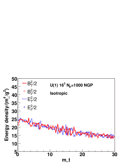
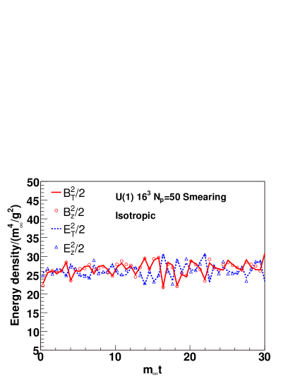
Figure 1: Time evolution of the magnetic and electric energy densities for $U(1)$ gauge group and isotropic particle momentum distribution using the nearest-grid-point method (left) and smeared-particles (right).

Full 3d-3v simulations, however, require improved algorithms since 3d lattices have many more sites and the NGP method becomes computationally too expensive. In Fig. 1 (left), the time evolution of the field energy densities on a $16^{3}$ lattice with $N_{p}=1000$ test-particles per site are shown. Despite the large number of particles, there seems to be an anomalous damping of the fields with the NGP method. We naively expect that to achieve the same accuracy as for a one-dimensional lattice, $N_{p}$ would have to increase exponentially with the number of spatial dimensions: $N_{p}^{3d}\sim(N_{p}^{1d})^{3}$. This makes multi-dimensional NGP simulations practically impossible and forces one to consider methods for smoothing particle densities and currents.

III.2 Current smearing in electromagnetic PIC simulations

In Abelian plasmas it is common to employ smoothed currents for particle-in-cell (PIC) simulations Hockney and Eastwood (1981); Birdsall and Langdon (1985) in order to avoid numerical noise. The charge density at site $(i,j,k)$ is obtained by smearing 

$$\rho(i,j,k)=e\sum^{N_{p}}_{n=1}S_{i}(x_{n})S_{j}(y_{n})S_{k}(z_{n})~{}.$$ (18)

Here, $S$ is a form factor. For example, the first-order form factor (shape-factor) is

$$S^{1}_{i}(\xi)=\left\{\begin{array}[]{ll}1-|\xi-i|&\mathrm{for}\,|\xi-i|\leq 1,\\ 0&\mathrm{for}\,|\xi-i|>1\end{array}\right.$$ (19)

However, it is well known that if we naively define the current density at each grid point as

$$J_{\alpha}(i,j,k)=e\sum^{N_{p}}_{n=1}v_{\alpha,n}S_{i}(x_{n})S_{j}(y_{n})S_{k}(z_{n}),\quad\alpha=x,y,z,$$ (20)

then the continuity equation is not satisfied exactly Hockney and Eastwood (1981); Birdsall and Langdon (1985), requiring us to correct the electric field by solving the Poisson equation.

To avoid solving Poisson’s equation in each time step, several numerical techniques for solving the continuity equation have been developed Eastwood (1991); Eastwood et al. (1995); Buneman and Villasenor (1992); Esirkepov (2001); Umeda et al. (2003). For simplicity, we consider the 2d problem to explain how to satisfy local charge conservation in electromagnetism. We consider a particle moving from $(x_{1},y_{1})$ to $(x_{2},y_{2})$ during a time step $\Delta t$, i.e. $x_{2}=x_{1}+v_{x}\Delta t,\quad y_{2}=y_{1}+v_{y}\Delta t$. We also restrict ourselves to the case in which $(x_{2},y_{2})$ belongs to the same lattice site $(i,j)$. Charge conservation of the assigned current densities is realized with the procedure described by Eastwood Eastwood (1991),

$$J_{x}(i,j) = F_{x}(1-W_{y}),\qquad J_{x}(i,j+1)=F_{x}W_{y}~{},$$

$$J_{y}(i,j) = F_{y}(1-W_{x}),\qquad J_{y}(i+1,j)=F_{y}W_{x}~{},$$ (21)

where $(F_{x},F_{y})\equiv\bm{F}$ represents the charge flux

$$F_{x}=e\frac{x_{2}-x_{1}}{\Delta t}~{},\qquad F_{y}=e\frac{y_{2}-y_{1}}{\Delta t}~{}.$$ (22)

$W$ represents the first-order shape-factor corresponding to the linear weighting function defined at the midpoint between the starting point $(x_{1},y_{1})$ and the end point $(x_{2},y_{2})$

$$W_{x}=\frac{x_{1}+x_{2}}{2}-i~{},\qquad W_{y}=\frac{y_{1}+y_{2}}{2}-j~{}.$$ (23)

One can easily show that the lattice continuity equation

$$J_{x}(i,j)-J_{x}(i-1,j)+J_{y}(i,j)-J_{y}(i,j-1)=\frac{\rho^{t}(i,j)-\rho^{t+\Delta t}(i,j)}{\Delta t}\,,$$ (24)

is satisfied with the definition (21) of the current. When $(x_{2},y_{2})$ is a different lattice site than the original $(i,j)$ one, we use the ‘Zigzag scheme’ developed in Ref. Umeda et al. (2003). Much of the numerical noise is eliminated by such linear interpolation. Note that our current may in general be expressed as

$$J_{\alpha}(i,j,k)=e\sum^{N_{p}}_{n=1}v_{\alpha,n}S^{0}_{\alpha}(x_{n})S^{1}_{j}(y_{n})S^{1}_{k}(z_{n}),\quad\alpha=x,y,z,\quad\alpha\neq j,k,$$ (25)

which differs from (20) since $S^{0}_{\alpha}=dS^{1}_{\alpha}/dx_{\alpha}$; $S^{0}_{\alpha}$ is the “form factor” of the NGP method, i.e. $S^{0}_{\alpha}=1$ if the particle is in the corresponding lattice site, otherwise it is zero.

Finally, we note that the electromagnetic forces should be smeared in a similar way when a particle momentum is updated Eastwood (1991); Eastwood et al. (1995). Consider the time derivative of the total energy:

$$\frac{dE}{dt}=-\sum_{\text{lattice}}\bm{E}\cdot\bm{J}+\sum_{\text{particles}}q_{i}\,\bm{E}(\bm{x}_{i}(t))\cdot\bm{v}_{i}.$$ (26)

It is clear that the interpolation function for $\bm{E}$ should be the same as that for $\bm{J}$ in order to achieve good energy conservation in the simulation. The electric field $\bm{E}(\bm{x})$ at the particle position $\bm{x}$ is then obtained from

$$E_{\alpha}(\bm{x})=\sum_{\text{lattice}}S^{0}_{\alpha}S^{1}_{\beta}S^{1}_{\gamma}E_{\alpha}(i,j,k)~{},$$ (27)

while the magnetic field is given by

$$B_{\alpha}(\bm{x})=\sum_{\text{lattice}}S^{1}_{\alpha}S^{0}_{\beta}S^{0}_{\gamma}B_{\alpha}(i,j,k)~{}.$$ (28)

This is motivated by the relations $\bm{E}=-\dot{\bm{A}}$ and $\bm{B}=\nabla\times\bm{A}$. The momentum update itself is explained in appendix A.

In Fig. 1 (right) we show the $U(1)$ energy densities resulting from an isotropic run using $N_{p}=50$ smeared test-particles per site. As can be seen from this figure the smeared-particle result does not suffer from the anomalous damping seen with the NGP method. More importantly, this result was obtained using many fewer particles than would be required to obtain a stable result with the NGP method. Therefore the smeared-particle method makes three-dimensional particle-in-cell (PIC) simulations possible in practice.

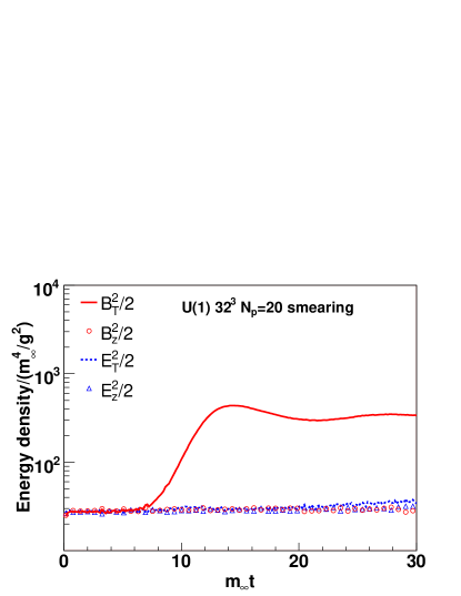
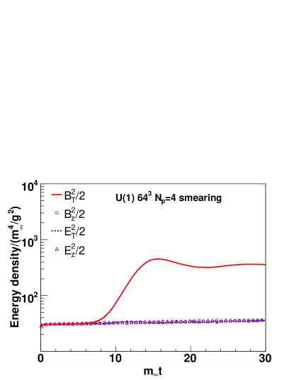
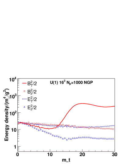
Figure 2: Time evolution of the field energy densities for $U(1)$ gauge group and anisotropic particle momentum distribution (10) on $16^{3}$, $32^{3}$ and $64^{3}$ lattices. Simulation parameters are $L=5$ fm, $p_{h}=16$ GeV, $g^{2}\,n_{g}=20$ fm^-3, $m_{\infty}=0.1$ GeV.

Fig. 2 shows the $U(1)$ field energy densities as a function of time for the anisotropic initial particle momentum distribution using both smeared particles and the NGP method. These simulations illustrate the improved accuracy of the smearing method as compared to the NGP method. Moreover, thanks to the smaller number of test-particles required by the smearing method we are now able to also run simulations on larger lattices. For these initial conditions, we observe an instability to transverse magnetic fields while all other field amplitudes are essentially constant over the depicted time interval. We also note that the evolution of the fields is essentially independent of the lattice spacing, indicating that only soft field modes are important for the dynamics of the instability in the Abelian theory. Below, we shall find that the situation is different for non-Abelian fields.

The growing fields deflect the particles if their momenta are not asymptotically large and as a consequence they aquire non-vanishing longitudinal momenta $p_{z}$ (c.f. section IV). We remark that PIC methods are not well suited for simulations of the extreme weak-field limit, where the particles propagate on nearly straight-line trajectories for a very long time. This is not due to physical but technical limitations: the weaker the fields, the more accurate the particle current $J^{\nu}$ needs to be (for example with respect to cancellations of positively and negatively charged particles etc.), as it represents a source-term in the field equations. High-precision currents, in turn, can only be achieved by employing a large number of test particles, driving up the computational time. In practice, the weakest fields for which simulations were feasible correspond to initial energy densities of about $0.1\,m^{4}_{\infty}/g^{2}$ for $U(1)$ and $\sim 10\,m^{4}_{\infty}/g^{2}$ for $SU(2)$ gauge group, respectively. The natural regime of applicability of PIC methods is when the separation between hard and soft degrees of freedom is not asymptotically large.

III.3 PIC simulations in non-Abelian gauge theories (CPIC)

A straightforward extension of the above-mentioned smearing method to the non-Abelian case would be to define the current as

$$J_{x}(i,j) = Q\frac{x_{2}-x_{1}}{\Delta t}(1-W_{y}),\qquad J_{x}(i,j+1)=Q_{y}\frac{x_{2}-x_{1}}{\Delta t}W_{y}~{},$$ (29)

$$J_{y}(i,j) = Q\frac{y_{2}-y_{1}}{\Delta t}(1-W_{x}),\qquad J_{y}(i+1,j)=Q_{x}\frac{y_{2}-y_{1}}{\Delta t}W_{x}~{},$$ (30)

where we define the parallel transport of the charge in 2d as 

$$Q_{x}\equiv U_{x}^{\dagger}(i,j)QU_{x}(i,j),\qquad Q_{y}\equiv U_{y}^{\dagger}(i,j)QU_{y}(i,j)~{}.$$ (31)

One can easily check that this satifies the lattice covariant continuity equation,

$$\dot{\rho}(i,j)=\sum_{x}U^{\dagger}_{x}(i-x)J_{x}(i-x)U_{x}(i-x)-J_{x}(i,j),$$ (32)

for sites $(i,j),(i+1,j),(i,j+1)$:

$$\dot{\rho}(i,j) = J_{x}(i,j)+J_{y}(i,j),$$ (33)

$$\dot{\rho}(i+1,j) = U^{\dagger}_{x}(i,j)J_{x}(i,j)U_{x}(i,j)-J_{y}(i+1,j),$$ (34)

$$\dot{\rho}(i,j+1) = U^{\dagger}_{y}(i,j)J_{y}(i,j)U_{y}(i,j)-J_{x}(i,j+1),$$ (35)

Eqs. (33), (34), (35) are consistent with the following definitions of the charge densities:

$$\rho(i,j) = Q(1-x)(1-y)~{},$$ (36)

$$\rho(i,j+1) = Q_{y}(1-x)y~{},$$ (37)

$$\rho(i+1,j) = Q_{x}x(1-y)~{}.$$ (38)

However, since a particle’s color charge depends on its path, so does $\rho(i+1,j+1)$ and we are not able to calculate it from the charge distribution itself. Rather, we directly employ covariant current conservation to determine the increment of charge at site $(i+1,j+1)$ within the time-step. This way, we can satisfy Gauss’s law in the non-Abelian case. The forces acting on a particle are determined by analogy to (27,28), except that the charges at neighboring sites is given by the expressions above.

Finally, we have to check that $\mbox{${\rm Tr}$}(Q^{2})$ is conserved by this smearing method. This is true when the lattice spacing $a$ is small, as the total charge of a particle is given by

$$Q_{0}=Q(1-x)(1-y)+Q_{x}x(1-y)+Q_{y}(1-x)y+[a_{p}Q_{xy}+(1-a_{p})Q_{yx}]xy~{},$$ (39)

where the $a_{p}$ depend on the path of a particle and $Q_{xy}=U^{\dagger}_{x}(i,j+1)Q_{y}U_{x}(i,j+1)$, $Q_{yx}=U^{\dagger}_{y}(i+1,j)Q_{x}U_{y}(i+1,j)$. If we require that $\mbox{${\rm Tr}$}(Q_{0}^{2})$ be constant, then the cross terms, for example $\mbox{${\rm Tr}$}(QQ_{x})$, have to vanish. This is true when $a$ is small, because $\mbox{${\rm Tr}$}(Q[A,Q])=0$:

$$\mbox{${\rm Tr}$}(QQ_{x})=\mbox{${\rm Tr}$}(Q(Q+iga[A_{x},Q]+{\cal O}(a^{2})))=\mbox{${\rm Tr}$}(Q^{2})+{\cal O}(a^{2}).$$ (40)

IV Results

IV.1 Electrodynamics

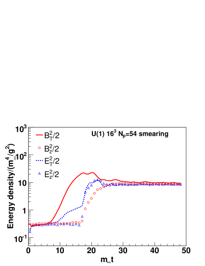
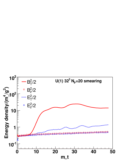
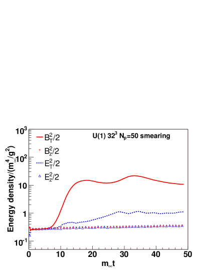
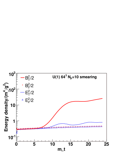
Figure 3: Time evolution of the field energy densities for $U(1)$ gauge group and anisotropic particle momentum distribution on various lattices. Simulation parameters in physical units are $L=5$ fm, $p_{h}=8$ GeV, $g^{2}\,n_{g}=100$ fm^-3, $m_{\infty}=0.3$ GeV.

In Fig. 3 we show simulation results for “weak” fields with initial energy density on the order of $0.1\,m_{\infty}^{4}/g^{2}$. For this case, we find that not only the transverse magnetic but also the transverse electric fields grow, albeit at a slower rate. Note that here, and throughout the manuscript, squared transverse field components denote averages of squares of $x$- and $y$-components: $B_{T}^{2}=(B_{x}^{2}+B_{y}^{2})/2$, $E_{T}^{2}=(E_{x}^{2}+E_{y}^{2})/2$. For the $16^{3}$ lattice there is a very sudden growth of all field components at $t\simeq 16\,m^{-1}_{\infty}$ which we deem unphysical since we do not expect equipartitioning of transverse and longitudinal fields; this is an example for the problems which arise in PIC simulations when the fields are very weak and the currents are not sufficiently stable. Indeed, this numerical instability disappears on larger lattices with more test-particles. The longitudinal field components are now essentially constant and only the transverse components grow. The time where the instability for the transverse magnetic fields sets in, as well as their growth rate and saturation point is quite similar for the $32^{3}$ and $64^{3}$ lattices.

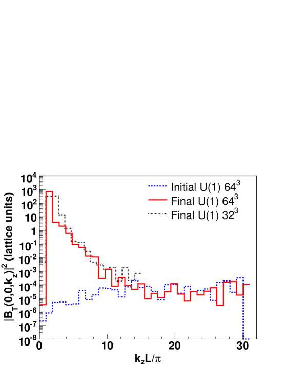
Figure 4: Fourier transform of the tranverse magnetic field from Fig. 3.

The slope of the exponential growth of $B_{T}^{2}$ is about half that predicted by the hard-loop approximation ($=\sqrt{2}\,m_{\infty}$ for the field energy density) which indicates that non-linear effects are not completely negligible. This is also apparent from the much slower growth of $E_{T}$ as compared to $B_{T}$ and in the Fourier transform of the transverse magnetic field shown in Fig. 4 which illustrates the spectrum of unstable modes. In the linear approximation, the spectrum of unstable modes for an extreme particle anisotropy extends to $k_{\rm max}\sim m_{\infty}/\theta$, where $\theta$ denotes the typical angular width of the particle momentum distribution. For our initial condition (10) $\theta=0$ at $t=0$ but grows to $\sim 10^{-3}$ during the short initial transient time before the onset of rapid field growth (see below). However, for the full non-linear solution we do not observe such a broad band of instability, modes above $k\simeq 10\pi/L$ are clearly stable. (We note also that the spectrum is not very sensitive to the lattice spacing, which indicates that this cutoff is not a lattice artifact.) This might be related to the fact that in our simulations $\theta$ increases only little and $k_{\rm max}$ is not very much smaller than the particle scale $p_{h}$. Therefore, it is likely that back-reaction only allows growth of modes with $k\ll k_{\rm max}$.

IV.2 Chromodynamics

We now turn to simulations for the non-Abelian $SU(2)$ gauge group. 3d-3v simulations within the hard-loop approximation show that the exponential growth of transverse magnetic and electric fields saturates at the scale $m_{\infty}^{2}/g$ due to field self-interactions  Arnold et al. (2005); Rebhan et al. (2005). While we can not address such weak fields with PIC methods for $SU(2)$, we focus here on non-Abelian plasma dynamics beyond the hard-loop approximation for initial field energy densities of $\sim 10\,m_{\infty}^{4}/g^{2}$ and above.

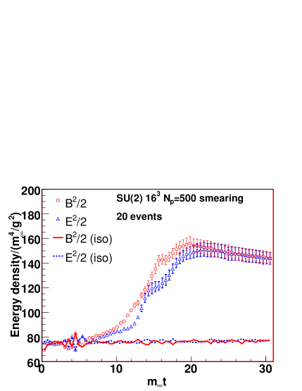
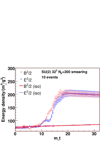
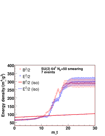
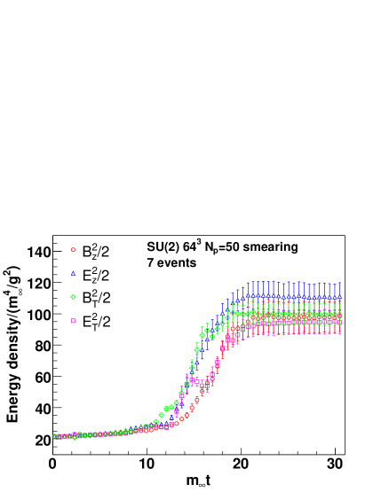
Figure 5: Time evolution of the field energy densities for $SU(2)$ gauge group and anisotropic initial particle momentum distributions. Simulation parameters are $L=5$ fm, $p_{\rm hard}=16$ GeV, $g^{2}\,n_{g}=10/$fm³, $m_{\infty}=0.1$ GeV.

Fig. 5 shows results obtained on various lattices. In each case the initial condition was taken to be Gaussian random chromoelectic fields which were “low-pass” filtered such that only the lower half of available lattice modes were populated. Note that in Fig. 5 the energy densities are plotted on a linear rather than logarithmic scale. Runs with an isotropic particle distribution are shown in each panel as an indication of our numerical accuracy (error bars are not indicated for the isotropic runs). The isotropic runs show nearly constant fields over the time interval $t\leq 30\,m^{-1}_{\infty}$. From these figures we observe that after a period of rapid growth both electric and magnetic fields settle to an essentially constant energy density.

Hence, we confirm that for 3d-3v simulations, even beyond the hard-loop approximation, the time evolution of non-Abelian fields stronger than $\sim m_{\infty}^{4}/g^{2}$ differs from that in the (effectively Abelian) extreme weak-field limit. In particular, a sustained exponential growth is absent even during the stage where overall the backreaction on the particles is weak. It should be emphasized, in fact, that for very strong anisotropies a linear analysis predicts that the exponential field growth (in the weak-field situation) could perhaps continue until $B^{2}\sim m_{\infty}^{4}/g^{2}/\Delta\theta^{2}$, with $\Delta\theta^{2}=p_{z}^{2}/p_{T}^{2}$ Arnold and Moore (2006a). For our initial condition (10), $\Delta\theta^{2}=0$ at $t=0$ but grows to ${\cal O}(10^{-3})$ during the initial transient time with constant fields ($t\,m_{\infty}\mbox{\raisebox{-2.58334pt}{$\stackrel{{\scriptstyle<}}{{\sim}}$}}\>10$ in Fig. 5) due to deflection of the particles. However, such strong fields are not seen in our PIC simulations. This may be related to the above-mentioned back-reaction effects which prevent instability of modes near $k_{\rm max}\sim m_{\infty}/\Delta\theta$.

The results shown in Fig. 5 indicate a sensitivity to hard field modes at the ultra-violet end of the Brioullin zone, $k={\cal O}(a^{-1})$, in contrast to the $U(1)$ simulations shown above and to earlier 1d-3v $SU(2)$ simulations Dumitru and Nara (2005, 2006); Nara (2006). The energy density contained in the fields at late times increases by a factor of 1.5 when going from a $16^{3}$ to $32^{3}$ to $64^{3}$ lattice with the same physical size $L$. Hence, the dynamics of $SU(2)$ instabilities seen here is not dominated entirely by a band of unstable modes in the infrared but clearly involves a cascade of energy from those modes to a harder scale $\Lambda$ Arnold and Moore (2006b). However, the simulations shown in Fig. 5 indicate that $\Lambda(t)$ grows to ${\cal O}(a^{-1})$ during the period of rapid growth of the field energy density; otherwise, the final field energy density would not depend on the lattice spacing.

Note that in our PIC simulations the total energy of particles and fields is conserved, hence $\Lambda(t)$ can not grow arbitrarily large if the energy density of the fields is UV sensitive. In three spatial dimensions, this is the case whenever the occupation number of hard field modes drops more slowly than $\sim 1/k^{4}$. The analysis of ref. Arnold and Moore (2006b), for example, suggests a $\sim 1/k^{2}$ fall-off near $k\sim\Lambda$, which indeed corresponds to a quadratically divergent energy density as $\Lambda\to\infty$. A different analysis Mueller et al. (2006) suggest a $\sim 1/k$ spectrum.

Although energy conservation will eventually stop the growth of the fields as the lattice spacing decreases towards the continuum, it does not solve the following problem. When $\Lambda(t)\sim 1/a$, the hard field modes have reached the momentum scale of the particles, $p_{h}={\cal O}(a^{-1})$, and so the clean separation of scales is lost, on which the approach (1,2) is based. In fact, since the occupation number (or phase space density) at that scale is of order 1 or less by construction, it is inappropriate to describe modes at that scale as a classical field. Those perturbative modes should be converted dynamically into particles at a lower scale $\Lambda_{f\to p}\ll 1/a$ so that the field energy density and the entire coupled field-particle evolution is independent of the artificial lattice spacing. We hope to be able to study this question in the future.

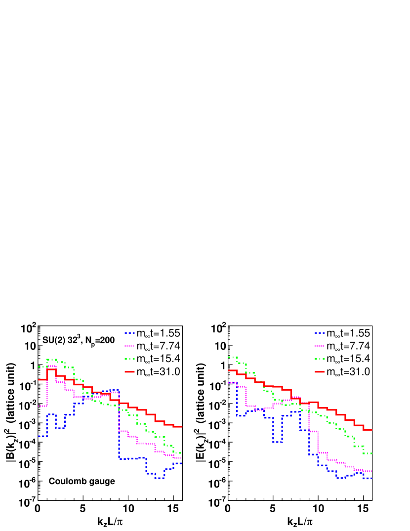
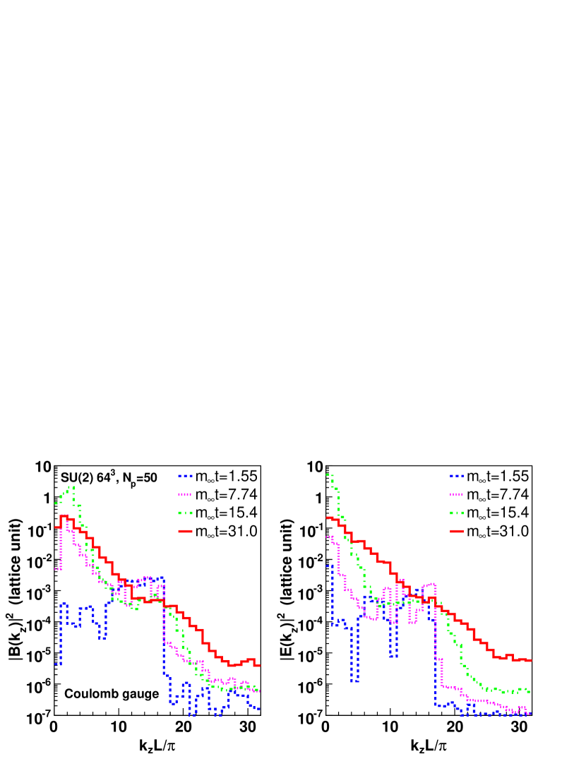
Figure 6: Squares of the Fourier transformed (color-) electric and magnetic fields in Coulomb gauge (lattice units) at four different times. Upper (lower) panels correspond to $32^{3}$ ($64^{3}$) lattices. Simulation parameters are the same as for Fig. 5. Note that $\pi/L\approx m_{\infty}$.

In Fig. 5 (lower right panel) we have also plotted the tranverse and longitudinal contributions to the electric and magnetic energy densities as a function of time. From this figure we see that at late times the distribution of field energy obtained from our 3d-3v $SU(2)$ PIC simulations is approximately isotropic. In contrast, for the 1d-3v and 3d-3v $U(1)$ PIC simulations and the 1d-3v $SU(2)$ CPIC simulations Dumitru and Nara (2005, 2006); Nara (2006) transverse magnetic fields dominate, corresponding to an energy-momentum tensor of the form $T^{00}_{\rm field}\approx T^{zz}_{\rm field}$ (and $T^{xx}_{\rm field}+T^{yy}_{\rm field}\approx 0$). However, we find that with our 3d-3v $SU(2)$ CPIC simulations the energy transfered to “hard” field modes is distributed isotropically, regardless of the strong residual anisotropy of the particle momenta. The approximate isotropy of the field energy densities is also seen in HL simulations of strongly anisotropic plasmas (see below).

In Fig. 6 we show $\bm{E}^{a}(\bm{k})\cdot\bm{E}^{a}(-\bm{k})$ and $\bm{B}^{a}(\bm{k})\cdot\bm{B}^{a}(-\bm{k})$ (field spectra) as functions of $k_{z}$ at $k_{x}=k_{y}=0$. The field configurations at the corresponding time were gauge transformed to satisfy Coulomb gauge, $\partial_{i}A^{i}=0$ in continuum notation. The Figure shows that before the onset of the rapid field growth from Fig. 5 there is a relatively slow build-up of UV modes, in qualitative agreement with the discussion in ref. Arnold and Moore (2006b). Also note the strong growth of the soft (unstable) field modes at early times. This is the stage where the field evolution is independent of the lattice spacing. However, during the period of steep growth from Fig. 5 the energy drained from the particles quickly avalanches from IR to UV field modes and the distribution over $k$ becomes quite broad. We attribute this avalanche to the UV to the self-interaction of the Yang-Mills fields since it is not observed for Abelian $U(1)$ fields (Fig. 4) even for extreme particle anisotropies.

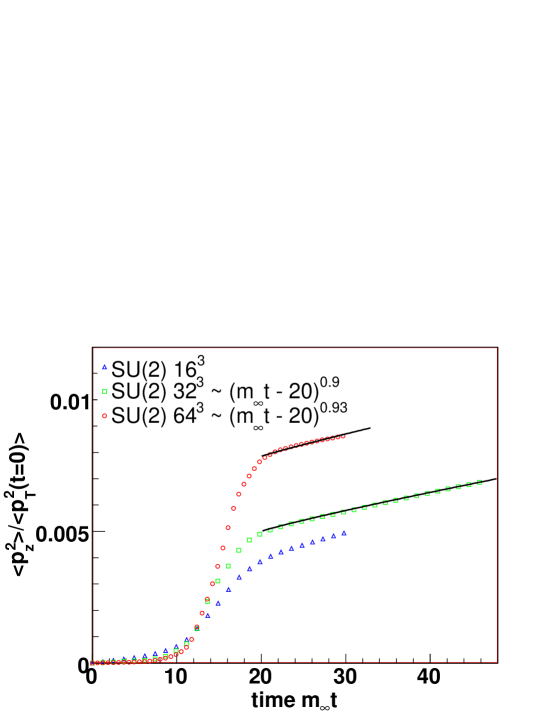
Figure 7: Broadening of the longitudinal particle momentum distribution for the simulations from Fig. 5. The line represents the power-law fit from eq. (42).

Fig. 7 depicts the time evolution of the typical longitudinal particle momentum. The broadening of the longitudinal distribution during the initial transient $t\,m_{\infty}\mbox{\raisebox{-2.58334pt}{$\stackrel{{\scriptstyle<}}{{\sim}}$}}\>10$ is independent of the lattice spacing. During the stage of steep field growth, $p_{z}$ broadens more rapidly, especially for the finer $64^{3}$ lattice. Since

$$\langle p_{z}^{2}\rangle\sim t\,\frac{dN_{scatt}}{dt}\,q_{z}^{2}~{},$$ (41)

with $q_{z}$ the typical momentum transfer in $z$-direction and ${dN_{scatt}}/{dt}$ the collision rate of particles with the field modes, it follows that during this stage either the scattering rate and/or the typical momentum transfer increase. This observation (and the fact that the effect is much stronger for the $64^{3}$ lattice) is consistent with the idea that during this stage the UV-cutoff $\Lambda(t)$ for the classical field grows to ${\cal O}(a^{-1})$.

A power-law fit to the late-time evolution of $\langle p_{z}^{2}\rangle$ of the form

$${\frac{\langle p_{z}^{2}\rangle}{\langle p_{x}^{2}+p_{y}^{2}\rangle}}\propto t^{\alpha}~{},$$ (42)

yields $\alpha\simeq 1$, corresponding to a random walk of the particles in $p_{z}$ with constant collision rate and average momentum transfer. In an expanding metric, this should then lead to a $\sim\tau^{-1/4}$ drop of the typical $p_{z}$, as argued by Bödeker Bödeker (2005) (see also section V in Arnold and Moore (2006a)). Hence, the anisotropy of the hard modes which develops in the early stage of a heavy-ion collision due to the rapid longitudinal expansion should be somewhat smaller than expected within the original “bottom-up” scenario Baier et al. (2001), which predicted $\surd\langle p_{z}^{2}\rangle\sim\tau^{-1/3}$.

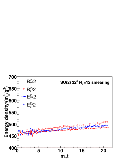
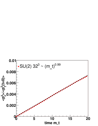
Figure 8: Left: field evolution for stronger initial fields. Right: evolution of the average longitudinal particle momentum. The line represents the power-law fit from eq. (42). The remaining simulation parameters are $p_{h}=16$ GeV, $g^{2}\,n_{g}=10$/fm³, $L=5$ fm, as before.

For even stronger initial fields, we find that the growth rate of the electric and magnetic fields and the dependence on the lattice spacing diminishes. Only a very mild linear growth remains over time spans which we can access in our simulations, see Fig. 8. A power-law fit of the form (42) again shows that the variance of the longitudinal momentum distribution grows linearly in time, corresponding to a random walk of the particles in $p_{z}$ with constant scattering rate (off the field modes) and typical momentum transfer.

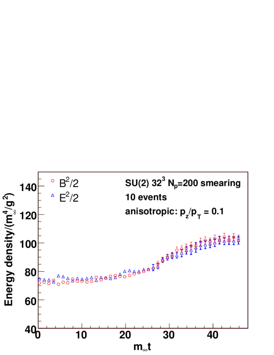
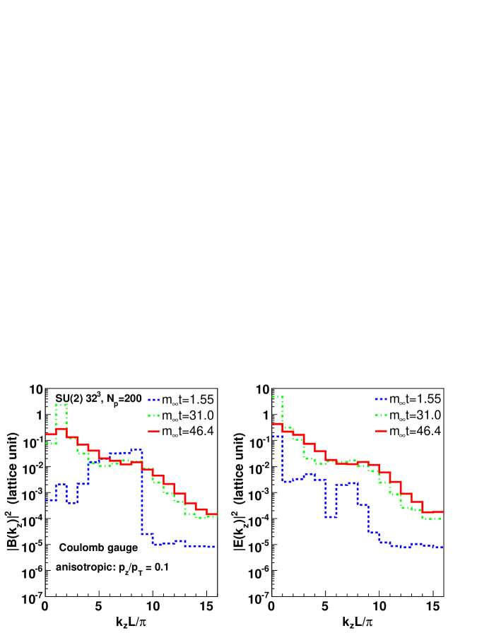
Figure 9: Field evolution for moderate initial anisotropy, $\sqrt{\langle p_{z}^{2}\rangle/\langle p_{T}^{2}\rangle}=10\%$. The remaining simulation parameters are the same as in Fig. 5. Top: field energy density as a function of time. Bottom: Fourier transformed color-fields (in Coulomb gauge) at different times.

We have also performed a simulation with a more moderate initial anisotropy of $\sqrt{\langle p_{z}^{2}\rangle/\langle p_{T}^{2}\rangle}=10\%$, replacing the function $\delta(p_{z})$ in (10) by an exponential $\sim\exp(-10\,|p_{z}|/p_{h})$. The time evolution of the fields and of their Fourier transform is shown in Fig. 9. As expected, the onset of field growth is delayed, by roughly a factor of two, as compared to the simulation with extreme particle anisotropy. Also, the intermediate rapid growth of the fields is weakened since the rate of energy transfer from particles to fields is now lower. Nevertheless, even for this run with more moderate anisotropy, we observe that the Fourier spectrum flattens somewhat at late times (when the growth saturates); it actually resembles the final spectrum from Fig. 6 although the angular width of the particle momentum distribution is now much larger.

Comparison with hard-loop results

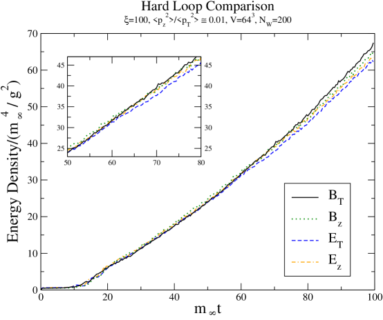
Figure 10: Field evolution for moderate initial anisotropy as obtained from numerical solution of hard-loop effective theory Rebhan et al. (2005).

In Fig. 10 we present the dependence of the energy densities obtained by solving the soft-field equations of motion in the hard-loop approximation Rebhan et al. (2005) for the case of $\sqrt{\langle p_{z}^{2}\rangle/\langle p_{T}^{2}\rangle}\sim 0.1$. For this simulation the initial condition has no fields, but instead has finite fluctuations of the auxilliary $W$ fields which induce field fluctuations with typical initial energy density ${\cal E}\sim 0.5\,m_{\infty}^{4}/g^{2}$ at early times (for details of the initial condition and numerical algorithm used see Ref. Rebhan et al. (2005)). Note that if one makes the same run with an isotropic hard particle distribution the fields remain isotropic and show no signs of growth.

As can be seen from Fig. 10 there is an initial period where no field growth occurs, similar to Fig. 9. At $m_{\infty}t\sim 10$ all field components begin to grow isotropically in the hard-loop simulation. They then grow approximately linearly and isotropically for the duration of the run. At late times one can see a slight curvature upwards suggesting a faster than linear growth. This curvature is related to the finite discretizations used in both space-time and velocity space. Improving these discretizations or damping high angular momentum modes Arnold et al. (2005) extends the region in time over which the linear behavior is observed. The inset of Fig. 10 shows the dependence of the field energy densities at late times when the magnitudes are comparable to those shown in Fig. 9. Also, similar to the CPIC results we see that the energy densities obtained in the hard-loop simulation are approximately isotropic.

V Discussion

We have presented numerical solutions of coupled particle-field dynamics in Abelian and non-Abelian gauge theories beyond the HL approximation. Such plasmas exhibit collective instabilities when the distribution of particles in momentum space is anisotropic (we restrict ourselves to an oblate distribution here). However, in the regime where field self-interactions can not be neglected, corresponding to field strengths of order $\sim m_{\infty}^{2}/g$ and above, the evolution in chromodynamics is rather different from that in Abelian plasmas. Most remarkably, for the initial conditions employed here, we do not observe a period of sustained exponential growth of the soft fields. This is because the field modes can interact directly and so the energy drained by the instability from the hard particles does not remain in unstable modes for a sufficiently long time.

The transition from exponential to linear growth at the scale $m_{\infty}^{2}/g$ has been seen previously in 3d-3v simulations within the HL approximation Arnold et al. (2005); Rebhan et al. (2005). It appears that if the particles exhibit only weak anisotropy, that the HL approach could be continued until very late times since hard field modes are populated very slowly. However, for moderate anisotropies the instability is also affected more easily by collisions among the particles Schenke et al. (2006) and by the rapid longitudinal expansion encountered in relativistic heavy-ion collisions Romatschke and Rebhan (2006).

For very anisotropic particle momentum distributions we find here that the evolution differs significantly for field strengths of order $m_{\infty}^{2}/g$ and above, even if overall the back-reaction on the hard particle modes is small. After some initial transient time, we observe a short period of rapid growth of soft electric and magnetic fields followed by an avalanche of energy into the UV. As long as the energy of the classical Yang-Mills fields is still much less than that of the particles, this avalanche proceeds to the smallest length scales, namely the lattice spacing $a$, before reaching a steady-state distribution. Since $1/a$ will eventually reach $p_{h}$ as one takes the continuum limit, the loss of a clear separation of scales between soft and hard degrees of freedom could perhaps be viewed as (partial) “classical decay” of the field into particles. To understand what happens then requires us to go beyond the Wong-Yang-Mills equations, which rely on such a separation of scales. We also point out that the energy-momentum tensor of the fields is nearly isotropic, while Weibel instabilities seen in $U(1)$ and 1d-3v $SU(2)$ simulations lead to dominance of transverse magnetic fields.

If the initial field energy density is rather high, of order $(10^{2}-10^{3})\,m^{4}_{\infty}/g^{2}$, we do not observe an instability with rapid growth of the fields. In this case, the mean-square width of the longitudinal particle distribution grows linearly in time. This corresponds to a random walk with constant scattering rate (from the field fluctuations) and typical momentum transfer. For even stronger initial fields with energy density comparable to that of the particles, $\sim p_{h}\,n_{g}$, we of course expect a very rapid isotropization of the particle pressure, see e.g. refs. Dumitru and Nara (2005, 2006); Nara (2006).

Our simulations indicate that it could be important to implement a dynamical field to particle conversion at a scale $\Lambda_{f\to p}<p_{h}$ to avoid that field and particle degrees of freedom overlap. This might lead to a continuous “cycle” of energy transfer from the anisotropic particles to soft field modes which then quickly re-emerges at that scale in isotropic form. The cycle should continue until all particle momenta are isotropic. Theoretically, it also remains to be understood why the energy avalanche from soft to hard field modes occurs so rapidly. An independent analytical discussion of energy transfer to small length scales in QCD has been recently given in ref. Mueller et al. (2006). In the future, we intend to perform more quantitative studies and verify the matching to the “bottom-up” solution for particle-field thermalization Mueller et al. (2005). To do so, however, requires us to also allow for longitudinal expansion of the lattice and to include hard elastic and inelastic scattering of particles.

Appendix A Momentum update

We consider the discretization of the equation

$$\frac{d\bm{p}}{dt}=gQ^{a}(\bm{E}^{a}+\bm{v}\times\bm{B}^{a}).$$ (43)

The difference form of the equation is

$$\frac{\bm{p}(t+\Delta t/2)-\bm{p}(t-\Delta t/2)}{\Delta t}=gQ^{a}\left(\bm{E}^{a}(t)+\frac{\bm{p}(t+\Delta t/2)+\bm{p}(t-\Delta t/2)}{2}\times\frac{\bm{B}^{a}(t)}{e(t)}\right)$$ (44)

Eq.(44) can be solved by the Buneman-Boris method Hockney and Eastwood (1981); Birdsall and Langdon (1985) as follows:

$$\bm{p}(t) = \bm{p}(t-\Delta t/2)+\frac{\Delta t}{2}\bm{E}(t),$$ (45)

$$e(t) = |\bm{p}(t)|,$$ (46)

$$\bm{p}^{\prime}(t) = \bm{p}(t)+\frac{\Delta t}{2}\bm{p}(t)\times\frac{\bm{B}(t)}{e(t)},$$ (47)

$$\bm{p}_{2}(t) = \bm{p}(t)+\frac{2}{1+(\bm{B}/e(t)\Delta t/2)^{2}}\frac{\Delta t}{2}\bm{p}^{\prime}(t)\times\frac{\bm{B}(t)}{e(t)},$$ (48)

$$\bm{p}(t+\Delta t/2) = \bm{p}_{2}(t)+\frac{\Delta t}{2}\bm{E}(t),$$ (49)

where $\bm{E}\equiv gQ^{a}\bm{E}^{a}$ and $\bm{B}\equiv gQ^{a}\bm{B}^{a}$. This scheme is time reversible and the overall momentum integration is accurate to second-order in the time step.

References

- Mueller (2003) A. H. Mueller, Nucl. Phys. A715, 20 (2003), eprint hep-ph/0208278.
- Iancu and Venugopalan (2003) E. Iancu and R. Venugopalan (2003), eprint hep-ph/0303204.
- McLerran (2005) L. McLerran, Nucl. Phys. A752, 355 (2005).
- Baier et al. (2001) R. Baier, A. H. Mueller, D. Schiff, and D. T. Son, Phys. Lett. B502, 51 (2001), eprint hep-ph/0009237.
- Mrówczyński (1993) S. Mrówczyński, Phys. Lett. B314, 118 (1993).
- Mrówczyński (1994) S. Mrówczyński, Phys. Rev. C49, 2191 (1994).
- Mrówczyński (1997) S. Mrówczyński, Phys. Lett. B393, 26 (1997), eprint hep-ph/9606442.
- Romatschke and Strickland (2003) P. Romatschke and M. Strickland, Phys. Rev. D68, 036004 (2003), eprint hep-ph/0304092.
- Arnold et al. (2003) P. Arnold, J. Lenaghan, and G. D. Moore, JHEP 08, 002 (2003), eprint hep-ph/0307325.
- Romatschke and Strickland (2004) P. Romatschke and M. Strickland, Phys. Rev. D70, 116006 (2004), eprint hep-ph/0406188.
- Mrówczyński et al. (2004) S. Mrówczyński, A. Rebhan, and M. Strickland, Phys. Rev. D70, 025004 (2004), eprint hep-ph/0403256.
- Romatschke and Venugopalan (2005) P. Romatschke and R. Venugopalan (2005), eprint hep-ph/0510292.
- Romatschke and Venugopalan (2006a) P. Romatschke and R. Venugopalan, Phys. Rev. Lett. 96, 062302 (2006a), eprint hep-ph/0510121.
- Romatschke and Venugopalan (2006b) P. Romatschke and R. Venugopalan (2006b), eprint hep-ph/0605045.
- Arnold et al. (2005) P. Arnold, G. D. Moore, and L. G. Yaffe, Phys. Rev. D72, 054003 (2005), eprint hep-ph/0505212.
- Rebhan et al. (2005) A. Rebhan, P. Romatschke, and M. Strickland, JHEP 09, 041 (2005), eprint hep-ph/0505261.
- Romatschke and Rebhan (2006) P. Romatschke and A. Rebhan (2006), eprint hep-ph/0605064.
- Krasnitz and Venugopalan (1999) A. Krasnitz and R. Venugopalan, Nucl. Phys. B557, 237 (1999), eprint hep-ph/9809433.
- Krasnitz and Venugopalan (2000) A. Krasnitz and R. Venugopalan, Phys. Rev. Lett. 84, 4309 (2000), eprint hep-ph/9909203.
- Krasnitz and Venugopalan (2001) A. Krasnitz and R. Venugopalan, Phys. Rev. Lett. 86, 1717 (2001), eprint hep-ph/0007108.
- Krasnitz et al. (2001) A. Krasnitz, Y. Nara, and R. Venugopalan, Phys. Rev. Lett. 87, 192302 (2001), eprint hep-ph/0108092.
- Krasnitz et al. (2003a) A. Krasnitz, Y. Nara, and R. Venugopalan, Nucl. Phys. A717, 268 (2003a), eprint hep-ph/0209269.
- Krasnitz et al. (2003b) A. Krasnitz, Y. Nara, and R. Venugopalan, Nucl. Phys. A727, 427 (2003b), eprint hep-ph/0305112.
- Krasnitz et al. (2003c) A. Krasnitz, Y. Nara, and R. Venugopalan, Phys. Lett. B554, 21 (2003c), eprint hep-ph/0204361.
- Lappi (2003) T. Lappi, Phys. Rev. C67, 054903 (2003), eprint hep-ph/0303076.
- Lappi and McLerran (2006) T. Lappi and L. McLerran (2006), eprint hep-ph/0602189.
- Fries et al. (2006) R. J. Fries, J. I. Kapusta, and Y. Li (2006), eprint nucl-th/0604054.
- Arnold and Moore (2006a) P. Arnold and G. D. Moore, Phys. Rev. D73, 025006 (2006a), eprint hep-ph/0509206.
- Arnold and Moore (2006b) P. Arnold and G. D. Moore, Phys. Rev. D73, 025013 (2006b), eprint hep-ph/0509226.
- Kelly et al. (1994a) P. F. Kelly, Q. Liu, C. Lucchesi, and C. Manuel, Phys. Rev. Lett. 72, 3461 (1994a), eprint hep-ph/9403403.
- Kelly et al. (1994b) P. F. Kelly, Q. Liu, C. Lucchesi, and C. Manuel, Phys. Rev. D50, 4209 (1994b), eprint hep-ph/9406285.
- Blaizot and Iancu (1999) J.-P. Blaizot and E. Iancu, Nucl. Phys. B557, 183 (1999), eprint hep-ph/9903389.
- Matinyan et al. (1988) S. G. Matinyan, E. B. Prokhorenko, and G. K. Savvidy, Nucl. Phys. B298, 414 (1988).
- Kawabe and Ohta (1990) T. Kawabe and S. Ohta, Phys. Rev. D41, 1983 (1990).
- Biro et al. (1994) T. S. Biro, C. Gong, B. Müller, and A. Trayanov, Int. J. Mod. Phys. C5, 113 (1994), eprint nucl-th/9306002.
- Wong (1970) S. K. Wong, Nuovo Cim. A65S10, 689 (1970).
- Heinz (1983) U. W. Heinz, Phys. Rev. Lett. 51, 351 (1983).
- Laine and Manuel (2002) M. Laine and C. Manuel, Phys. Rev. D65, 077902 (2002), eprint hep-ph/0111113.
- Ambjørn et al. (1991) J. Ambjørn, T. Askgaard, H. Porter, and M. E. Shaposhnikov, Nucl. Phys. B353, 346 (1991).
- Hu and Müller (1997) C. R. Hu and B. Müller, Phys. Lett. B409, 377 (1997), eprint hep-ph/9611292.
- Moore et al. (1998) G. D. Moore, C.-r. Hu, and B. Müller, Phys. Rev. D58, 045001 (1998), eprint hep-ph/9710436.
- Dumitru and Nara (2005) A. Dumitru and Y. Nara, Phys. Lett. B621, 89 (2005), eprint hep-ph/0503121.
- Dumitru and Nara (2006) A. Dumitru and Y. Nara, Eur. Phys. J. A29, 65 (2006), eprint hep-ph/0511242.
- Nara (2006) Y. Nara, Nucl. Phys. A774, 783 (2006), eprint nucl-th/0509052.
- Hockney and Eastwood (1981) R. W. Hockney and J. W. Eastwood, Computer Simulation Using Particles (McGraw-Hill, New York, 1981).
- Birdsall and Langdon (1985) C. K. Birdsall and A. Langdon, Plasma Physics via Computer Simulation (McGraw-Hill, New York, 1985).
- Eastwood (1991) J. W. Eastwood, Comput. Phys. Comm. 64, 252 (1991).
- Eastwood et al. (1995) J. W. Eastwood, W. Arter, N. J. Brealey, and R. Hockney, Comput. Phys. Comm. 87, 155 (1995).
- Buneman and Villasenor (1992) O. Buneman and J. Villasenor, Comput. Phys. Comm. 69, 306 (1992).
- Esirkepov (2001) T. Z. Esirkepov, Comput. Phys. Comm. 135, 144 (2001).
- Umeda et al. (2003) T. Umeda, Y. Omura, T. Tominaga, and H. Matsumoto, Comput. Phys. Comm. 156, 73 (2003).
- Mueller et al. (2006) A. H. Mueller, A. I. Shoshi, and S. M. H. Wong (2006), eprint hep-ph/0607136.
- Bödeker (2005) D. Bödeker, JHEP 10, 092 (2005), eprint hep-ph/0508223.
- Schenke et al. (2006) B. Schenke, M. Strickland, C. Greiner, and M. H. Thoma, Phys. Rev. D 73, 125004 (2006), eprint hep-ph/0603029.
- Mueller et al. (2005) A. H. Mueller, A. I. Shoshi, and S. M. H. Wong (2005), eprint hep-ph/0512045.