Abstract

We present the currently most accurate evaluation of the $W$ boson mass, $M_{W}$, in the Minimal Supersymmetric Standard Model (MSSM). The full complex phase dependence at the one-loop level, all available MSSM two-loop corrections as well as the full Standard Model result have been included. We analyse the impact of the different sectors of the MSSM at the one-loop level with a particular emphasis on the effect of the complex phases. We discuss the prediction for $M_{W}$ based on all known higher-order contributions in representative MSSM scenarios. Furthermore we obtain an estimate of the remaining theoretical uncertainty from unknown higher-order corrections.

1 Introduction

The relation between the massive gauge-boson masses, $M_{W}$ and $M_{Z}$, in terms of the Fermi constant, $G_{\mu}$, and the fine structure constant, $\alpha$, is of central importance for testing the electroweak theory. It is usually employed for predicting $M_{W}$ in the model under consideration. This prediction can then be compared with the corresponding experimental value. The current experimental accuracy for $M_{W}$, obtained at LEP and the Tevatron, is $\delta M_{W}=30\,\,\mathrm{MeV}$ (0.04%) [1, 2]. This experimental resolution provides a high sensitivity to quantum effects involving the whole structure of a given model. The $M_{W}$–$M_{Z}$ interdependence is therefore an important tool for discriminating between the Standard Model (SM) and any extension or alternative of it, and for deriving indirect constraints on unknown parameters such as the masses of the SM Higgs boson or supersymmetric particles, see Ref. [3] for a recent review. Within the SM the confrontation of the theory prediction and experimental result for the $W$ boson mass supplemented by the other precision observables yields an indirect constraint on the Higgs-boson mass, $M_{H}$, of $M_{H}=89^{+42}_{-30}\,\,\mathrm{GeV}$ with $M_{H}<175\,\,\mathrm{GeV}$ at the 95% C.L. [2]. Within the Minimal Supersymmetric Standard Model (MSSM) [4] the electroweak precision observables exhibit a certain preference for a relatively low scale of supersymmetric particles, see e.g. Refs. [5, 6].

The experimental precision on $M_{W}$ will further improve within the next years. The Tevatron data will reduce the experimental error to about $\delta M_{W}=20\,\,\mathrm{MeV}$ [7], while at the LHC an accuracy of about $\delta M_{W}=15\,\,\mathrm{MeV}$ [8] is expected. At the GigaZ option of a linear $e^{+}e^{-}$ collider, a precision of $\delta M_{W}=7\,\,\mathrm{MeV}$ can be achieved [9, 10].

A precise theoretical prediction for $M_{W}$ in terms of the model parameters is of utmost importance for present and future electroweak precision tests. Within the SM, the complete one-loop [11] and two-loop [12, 13, 14, 15, 16] results are known as well as leading higher-order contributions [17, 18, 19, 20, 21].

The theoretical evaluation of $M_{W}$ within the MSSM is not as advanced as in the SM. So far, the one-loop contributions have been evaluated completely [22, 23, 24, 25, 26], restricting however to the special case of vanishing complex phases (contributions to the $\rho$ parameter with non-vanishing complex phases in the scalar top and bottom mass matrices have been considered in Ref. [27]). At the two-loop level, the leading ${\cal O}(\alpha\alpha_{s})$ corrections [28, 29] and, most recently, the leading electroweak corrections of ${\cal O}(\alpha_{t}^{2})$, ${\cal O}(\alpha_{t}\alpha_{b})$, ${\cal O}(\alpha_{b}^{2})$to $\Delta\rho$ have been obtained [30, 31]. Going beyond the minimal SUSY model and allowing for non-minimal flavor violation the leading one-loop contributions are known [32].

In order to fully exploit the experimental precision for testing supersymmetry (SUSY) and deriving constraints on the supersymmetric parameters, it is desirable to have a prediction of $M_{W}$ in the MSSM at the same level of accuracy as in the SM. As a step into this direction, we perform in this paper a complete one-loop calculation of all contributions to $M_{W}$ in the MSSM with complex parameters (cMSSM), taking into account for the first time the full phase dependence and imposing no restrictions on the various soft SUSY-breaking parameters. We combine this result with the full set of higher-order contributions in the SM and with all available corrections in the MSSM. In this way we obtain the currently most complete result for $M_{W}$ in the MSSM. A public computer code based on our result for $M_{W}$ is in preparation.

We analyse the numerical results for $M_{W}$ for various scenarios in the unconstrained MSSM and for SPS benchmark scenarios [34]. The dependence of the result on the complex phases of the soft SUSY-breaking parameters is investigated. We estimate the remaining theoretical uncertainties from unknown higher-order corrections.

The outline of the paper is as follows. In Sect. 2 the basic relations needed for the prediction of $M_{W}$ are given and our conventions and notations for the different SUSY sectors are defined. In Sect. 3 the complete one-loop result $M_{W}$ including the full phase dependence of the complex MSSM parameters is obtained. The incorporation of all available higher-order corrections in the SM and the MSSM is described. The numerical analysis is presented in Sect. 4, where we also estimate the remaining theoretical uncertainties in the prediction for $M_{W}$. We conclude with Sect. 5.

2 Prediction for $M_{W}$ – basic entries

Muons decay to almost 100% into $e\nu_{\mu}\bar{\nu}_{e}$ [35]. Historically, this decay process was first described within Fermi’s effective theory. The muon decay rate is related to Fermi’s constant, $G_{\mu}$, by the defining equation

$$\Gamma_{\mu}=\frac{G_{\mu}^{2}m_{\mu}^{5}}{192\pi^{3}}\,F(\frac{m_{e}^{2}}{m_{\mu}^{2}})\left(1+\frac{3}{5}\frac{m_{\mu}^{2}}{M_{W}^{2}}\right)(1+\Delta_{\rm QED}),$$ (1)

with $F(x)=1-8x-12x^{2}\ln x+8x^{3}-x^{4}$. By convention, the QED corrections in the effective theory, $\Delta_{\rm QED}$, are included in eq. (1) as well as the (numerically insignificant) term $3m_{\mu}^{2}/(5M_{W}^{2})$ arising from the tree-level $W$ propagator. The precise measurement of the muon lifetime and the equivalently precise calculation of $\Delta_{\rm QED}$ [36, 37] thus provide the accurate value

$$G_{\mu}=(1.16637\pm 0.00001\times 10^{-5})\,\,\mathrm{GeV}^{-2}.$$ (2)

In the SM and in the MSSM, $G_{\mu}$ is determined as a function of the basic model parameters. The corresponding relation can be written as follows,

$$\frac{G_{\mu}}{\sqrt{2}}=\frac{e^{2}}{8\left(1-\frac{M_{W}^{2}}{M_{Z}^{2}}\right)M_{W}^{2}}\,(1+\Delta r).$$ (3)

The quantity $\Delta r$ summarizes the non-QED quantum corrections, since QED quantum effects are already included in the definition of $G_{\mu}$ according to eq. (1), which makes the evaluation of $\Delta r$ insensitive to infrared divergences. $\Delta r$ depends on all the model parameters, which enter through the virtual states of all particles in loop diagrams,

$$\Delta r=\Delta r(M_{W},M_{Z},m_{t},\alpha,\alpha_{s},\ldots,X)$$ (4)

with

$$X=M_{H^{\mathrm{SM}}}~{}~{}(\mathrm{SM}),$$

$$X=M_{h},M_{H},M_{A},M_{H^{\pm}},\tan\beta,M_{\tilde{f}},A_{f},m_{\tilde{\chi}^{0,\pm}},\dots~{}~{}\textup{(MSSM)},$$

and is hence a model-specific quantity. For each specification of the parameter set $X$, the basic relation (3) is fulfilled only by one value of $M_{W}$. This value can be considered the model-specific prediction of the $W$ mass, $M_{W}(X)$, providing a sensitive precision observable, with different results in the SM and in the MSSM. Comparing the prediction of $M_{W}$ with the experimental measurement leads to stringent tests of these models. Within the SM one can put bounds on the Higgs boson mass, which has so far not been directly measured experimentally. In the MSSM, $\Delta r$ and $M_{W}$ are sensitive to all the free parameters of the model, such as SUSY particle masses, mixing angles and couplings. The SUSY entries are briefly described below, thereby introducing also conventions and notations for the subsequent discussion.

gSfermions:

The mass matrix for the two sfermions of a given flavour, in the $\tilde{f}_{L},\tilde{f}_{R}$ basis, is given by

$${{\mathbf{M}}}_{\tilde{f}}=\begin{pmatrix}M_{L}^{2}+m_{f}^{2}&m_{f}\;X_{f}^{*}\\ m_{f}\;X_{f}&M_{R}^{2}+m_{f}^{2}\end{pmatrix},$$ (5)

with

$$M_{L}^{2} = M_{\tilde{F}}^{2}+M_{Z}^{2}\cos 2\beta\hskip 2.84526pt(I_{3}^{f}-Q_{f}s_{\mathrm{w}}^{2})$$

$$M_{R}^{2} = M_{\tilde{F}^{\prime}}^{2}+M_{Z}^{2}\cos 2\beta\hskip 2.84526ptQ_{f}s_{\mathrm{w}}^{2}$$ (6)

$$X_{f} = A_{f}-\mu^{*}\{\cot\beta\hskip 2.84526pt,\tan\beta\},$$

where $\{\cot\beta\hskip 2.84526pt,\tan\beta\}$ applies for up- and down-type sfermions, respectively, and $s_{\mathrm{w}}^{2}\equiv\sin^{2}\theta_{\rm W}=1-M_{W}^{2}/M_{Z}^{2}$. In the Higgs and scalar fermion sector of the cMSSM, $N_{f}+1$ phases are present, one for each $A_{f}$ and one for $\mu$, i.e. $N_{f}+1$ new parameters appear. As an abbreviation,

$$\phi_{A_{f}}\equiv\arg(A_{f})\,,$$ (7)

will be used. As an independent parameter one can trade $\phi_{A_{f}}$ for $\phi_{X_{f}}\equiv\arg(X_{f})$. The sfermion mass eigenstates are obtained by the transformation

$$\left(\begin{array}[]{c}\tilde{f}_{1}\\ \tilde{f}_{2}\end{array}\right)={{\mathbf{U}}_{\tilde{f}}}\left(\begin{array}[]{c}\tilde{f}_{L}\\ \tilde{f}_{R}\end{array}\right),$$ (8)

with a unitary matrix ${\mathbf{U}}_{\tilde{f}}$. The mass eigenvalues are given by

$$m_{\tilde{f}_{1,2}}^{2}=m_{f}^{2}+\frac{1}{2}\left[M_{L}^{2}+M_{R}^{2}\mp\sqrt{(M_{L}^{2}-M_{R}^{2})^{2}+4m_{f}^{2}|X_{f}|^{2}}~{}\right],$$ (9)

and are independent of the phase of $X_{f}$.

gHiggs bosons:

Contrary to the SM, in the MSSM two Higgs doublets are required. At the tree level, the Higgs sector can be described with the help of two independent parameters, usually chosen as the ratio of the two vacuum expectation values, $\tan\beta\equiv v_{2}/v_{1}$, and $M_{A}$, the mass of the ${\cal CP}$-odd $A$ boson. Diagonalisation of the bilinear part of the Higgs potential, i.e. the Higgs mass matrices, is performed via rotations by angles $\alpha$ for the ${\cal CP}$-even part and $\beta$ for the ${\cal CP}$-odd and the charged part. The angle $\alpha$ is thereby determined through

$$\tan 2\alpha=\tan 2\beta\;\frac{M_{A}^{2}+M_{Z}^{2}}{M_{A}^{2}-M_{Z}^{2}};\qquad-\frac{\pi}{2}<\alpha<0~{}.$$ (10)

One obtains five physical states, the neutral ${\cal CP}$-even Higgs bosons $h,H$, the ${\cal CP}$-odd Higgs boson $A$, and the charged Higgs bosons $H^{\pm}$. Furthermore there are three unphysical Goldstone boson states, $G^{0},G^{\pm}$. At lowest order, the Higgs boson masses can be expressed in terms of $M_{Z},M_{W}$, and $M_{A}$,

$$M_{h,H}^{2} = \frac{1}{2}\left[M_{A}^{2}+M_{Z}^{2}\mp\sqrt{(M_{A}^{2}+M_{Z}^{2})^{2}-4M_{A}^{2}M_{Z}^{2}\cos^{2}2\beta\hskip 2.84526pt}\right],$$

$$M_{H^{\pm}}^{2} = M_{A}^{2}+M_{W}^{2}.$$ (11)

Higher-order corrections, especially to $M_{h}$, however, are in general quite large. Therefore we use the results for the Higgs boson masses as obtained from the code FeynHiggs2.2 [38, 39, 40]; also the angle $\alpha$ is replaced by the effective mixing angle $\alpha_{\rm eff}$ in the improved Born approximation [41, 42].

gCharginos and neutralinos:

The physical masses of the charginos are determined by the matrix

$${\mathbf{X}}=\begin{pmatrix}M_{2}&\sqrt{2}\sin\beta\,M_{W}\\ \sqrt{2}\cos\beta\,M_{W}&\mu\end{pmatrix},$$ (12)

which contains the soft breaking term $M_{2}$ and the Higgsino mass term $\mu$, both of which may have complex values in the cMSSM. Their complex phases are denoted by

$$\phi_{M_{2}}\equiv{\rm arg}\left(M_{2}\right)~{}\ \ \textup{and}\ \ \phi_{\mu}\equiv{\rm arg}\left(\mu\right).$$ (13)

The physical masses are denoted as $m_{\tilde{\chi}^{\pm}_{1,2}}$ and are obtained by applying the diagonalisation matrices ${{{\mathbf{U}}}_{{\tilde{\chi}}^{\pm}}}$ and ${{{\mathbf{V}}}_{{\tilde{\chi}}^{\pm}}}$,

$${\bf U^{\ast}_{{\tilde{\chi}}^{\pm}}}{\mathbf{X}}{{{\mathbf{V}}}^{\dagger}_{{\tilde{\chi}}^{\pm}}}=\begin{pmatrix}m_{\tilde{\chi}^{\pm}_{1}}&0\\ 0&m_{\tilde{\chi}^{\pm}_{2}}\end{pmatrix}\,.$$ (14)

The situation is similar for the neutralino masses, which can be calculated from the mass matrix ($s_{\mathrm{w}}=\sin\theta_{\rm w}$, $c_{\mathrm{w}}=\cos\theta_{\rm w}$)

$${\mathbf{Y}}=\begin{pmatrix}M_{1}&0&-M_{Z}\,s_{\mathrm{w}}\cos\beta\,&M_{Z}\,s_{\mathrm{w}}\sin\beta\,\\ 0&M_{2}&\quad M_{Z}\,c_{\mathrm{w}}\cos\beta\,&M_{Z}\,c_{\mathrm{w}}\sin\beta\,\\ -M_{Z}\,s_{\mathrm{w}}\cos\beta\,&M_{Z}\,c_{\mathrm{w}}\cos\beta\,&0&-\mu\\ \quad M_{Z}\,s_{\mathrm{w}}\sin\beta\,&M_{Z}\,c_{\mathrm{w}}\sin\beta\,&-\mu&0\end{pmatrix}.$$ (15)

This symmetric matrix contains the additional complex soft-breaking parameter $M_{1}$, where the complex phase of $M_{1}$ is given by

$$\phi_{M_{1}}\equiv{\rm arg}\left(M_{1}\right).$$ (16)

The physical masses are denoted as $m_{\tilde{\chi}^{0}_{1,2,3,4}}$ and are obtained in a diagonalisation procedure using the matrix ${\mathbf{N}}_{\tilde{\chi}^{0}}$.

$${\mathbf{N}}_{\tilde{\chi}^{0}}^{\ast}{\mathbf{Y}}{\mathbf{N}}_{\tilde{\chi}^{0}}^{\dagger}=\begin{pmatrix}m_{\tilde{\chi}^{0}_{1}}&0&0&0\\ 0&m_{\tilde{\chi}^{0}_{2}}&0&0\\ 0&0&m_{\tilde{\chi}^{0}_{3}}&0\\ 0&0&0&m_{\tilde{\chi}^{0}_{4}}\end{pmatrix}.$$ (17)

At the two-loop level also the gluino enters the calculation of $M_{W}$. In our calculation below we will incorporate the full phase dependence of the complex parameters at the one-loop level, while we neglect the explicit dependence on the complex phases beyond the one-loop order. Accordingly, we take the soft SUSY-breaking parameter associated with the gluino mass, $M_{3}\equiv m_{\tilde{g}}$, which enters only at two-loop order, to be real.

3 Calculation of $\Delta r$

Our aim is to obtain a maximally precise and general prediction for $M_{W}$ in the MSSM. So far the one-loop result has been known only for the case of real SUSY parameters [24, 25]. In this section, we evaluate the complete one-loop result in the cMSSM with general, complex parameters and describe the incorporation of higher-order terms.

3.1 Complete one-loop result in the complex MSSM

Evaluation of the full one-loop results requires renormalisation of the tree-level Lagrangian. This introduces a set of one-loop counter terms, which contribute to the muon decay amplitude, in addition to the genuine one-loop graphs. At one-loop order, $\Delta r$ can be expressed in terms of the $W$ boson self-energy, vertex corrections (“vertex”), box diagrams (“box”), and counterterms for charge, mass, and field renormalisation as follows,

$$\Delta r^{(\alpha)} = \frac{\Sigma_{T}^{WW}(0)}{M_{W}^{2}}-\frac{\delta M_{W}^{2}}{M_{W}^{2}}+2\frac{\delta e}{e}-\frac{c_{\mathrm{w}}^{2}}{s_{\mathrm{w}}^{2}}\left(\frac{\delta M_{Z}^{2}}{M_{Z}^{2}}-\frac{\delta M_{W}^{2}}{M_{W}^{2}}\right)$$ (18)

$$+\frac{1}{2}\delta Z^{e}_{L}+\frac{1}{2}\delta Z^{\nu_{e}}_{L}+\frac{1}{2}\delta Z^{\mu}_{L}+\frac{1}{2}\delta Z^{\nu_{\mu}}_{L}+({\rm vertex})+({\rm box}),$$

where $\Sigma_{T}(q^{2})$ denotes the transverse part of a vector boson self-energy. The leading contributions to $\Delta r^{(\alpha)}$ arise from the renormalisation of the electric charge and the weak mixing angle (the last two terms in the first line of eq. (18)). The former receives large fermionic contributions from the shift in the fine structure constant due to light fermions, $\Delta\alpha\propto\log(m_{f}/M_{Z})$, a pure SM contribution. The latter involves the leading universal corrections induced by the mass splitting between fields in an isospin doublet [43],

$$\Delta\rho=\frac{\Sigma_{T}^{ZZ}(0)}{M_{Z}^{2}}-\frac{\Sigma_{T}^{WW}(0)}{M_{W}^{2}}.$$ (19)

In the SM $\Delta\rho$ reduces to the well-known quadratic term in the top-quark mass if the masses of the light fermions are neglected. In the MSSM $\Delta\rho$ receives additional sfermion contributions, in particular from the squarks of the third generation. The one-loop result for $\Delta r$ expressed in terms of $\Delta\alpha$ and $\Delta\rho$ reads

$$\Delta r^{{(\alpha)}}=\Delta\alpha-\frac{c_{\mathrm{w}}^{2}}{s_{\mathrm{w}}^{2}}\Delta\rho+\Delta r_{\rm rem}^{(\alpha)},$$ (20)

where $\Delta r_{\rm rem}^{(\alpha)}$ summarizes the remainder terms in eq. (18).

Throughout our calculation the on-shell renormalisation scheme is applied. In this scheme renormalisation conditions are imposed such that the particle masses are the poles of the propagators and the fields are renormalised by requiring unity residues of the poles. These conditions ensure that the $M_{W}$–$M_{Z}$ interdependence given by eq. (3) is a relation between the physical masses of the two gauge bosons. Applying the renormalisation conditions, the counterterms in eq. (18) can be expressed in terms of self-energies, and eq. (18) turns into

$$\Delta r^{(\alpha)} = \frac{\Sigma_{T}^{WW}(0)}{M_{W}^{2}}+({\rm vertex})+({\rm box})-\frac{{\rm Re}\,\Sigma_{T}^{WW}(M_{W}^{2})}{M_{W}^{2}}$$ (21)

$$+\Big{[}\frac{\partial\Sigma^{\gamma\gamma}_{T}(k^{2})}{\partial k^{2}}\Big{]}_{k^{2}=0}-\frac{s_{\mathrm{w}}}{c_{\mathrm{w}}}\frac{\Sigma^{\gamma Z}_{T}(0)}{M_{Z}^{2}}-\frac{c_{\mathrm{w}}^{2}}{s_{\mathrm{w}}^{2}}\,{\rm Re}\,\left[\frac{\Sigma^{ZZ}_{T}(M_{Z}^{2})}{M_{Z}^{2}}-\frac{\Sigma^{WW}_{T}(M_{W}^{2})}{M_{W}^{2}}\right]$$

$$-\Sigma^{e}_{L}(0)-\Sigma^{\mu}_{L}(0)-\Sigma^{\nu_{e}}_{L}(0)-\Sigma^{\nu_{\mu}}_{L}(0)\,,$$

where $\Sigma_{L}(q^{2})$ denotes the left-handed part of a fermion self-energy. The electron and muon masses are neglected in the fermion field renormalisation constants, which is possible since the only mass-singular virtual photon contribution is already contained in $\Delta_{\rm QED}$ of eq. (1) and is not part of $\Delta r$.

At the one-loop level one can divide the diagrams contributing to $\Delta r$ into four classes:

• SM-like contributions of quark and lepton loops in the gauge-boson self-energies, schematically depicted in Fig. 1;

• SUSY contributions of squark and slepton loops in the gauge-boson self-energies, depicted in Fig. 2;

• contributions from the Higgs and gauge boson sector, which contain besides self-energies (Figs. 3 and 4) also vertex and box graphs (Fig. 5).

• SUSY contributions involving neutralinos and charginos in self-energies, vertex graphs and box diagrams, see Figs. 6 and 7.

Figure 1: Generic lepton and quark one-loop diagram contributing to $\Delta r$ via gauge-boson self-energies; $V_{1},V_{2}=\gamma,Z,W^{\pm}$, $f_{1},f_{2}=\nu,l,u,d$.

Figure 2: Generic squark and slepton one-loop diagrams which contribute to $\Delta r$ via gauge-boson self-energies; $\tilde{f},\tilde{f}_{1},\tilde{f}_{2}=\tilde{\nu},\tilde{l},\tilde{u},\tilde{d}$.

Figure 3: Generic gauge-boson contributions to one-loop gauge-boson and fermion self-energies entering $\Delta r$ (the same diagrams as in the SM). The labels $l$ and $\nu$ in the fermion self-energy diagram stand for electron, muon and the corresponding neutrinos.

Figure 4: Generic contributions of MSSM Higgs bosons and Goldstone bosons to one-loop gauge-boson self-energies; $s,s_{1},s_{2}=h,H,A,H^{\pm},G^{0},G^{\pm}$.

Figure 5: Generic gauge-boson contributions to one-loop vertex and box diagrams entering $\Delta r$ (the same diagrams as in the SM). The labels $l$ and $\nu$ in the vertex diagrams stand for electron, muon and the corresponding neutrinos.

Figure 6: Generic neutralino/chargino contributions to gauge-boson (1) and fermion (2) self-energy diagrams. The labels $l$, $\nu$ in the fermion self-energy diagram stand for electron, muon and their corresponding neutrinos, and the labels $\tilde{l}$, $\tilde{\nu}$ indicate their respective superpartners.

Figure 7: Generic neutralino and chargino contributions to one-loop vertex and box diagrams entering $\Delta r$. The labels $l$, $\nu$ stand for electron, muon and their corresponding neutrinos, and the labels $\tilde{l}$, $\tilde{\nu}$ indicate their respective superpartners.

The calculation of the one-loop diagrams was performed in the dimensional regularisation [44] as well as the dimensional reduction scheme [45]. The analytical result for $\Delta r$ turned out to be independent of the choice of scheme.

Technically, the calculation was done with support of the Mathematica packages FeynArts [46, 47], OneCalc [48], and FormCalc [49]. A peculiarity among the box diagrams is the graph with a virtual photon, see diagram (4) in Fig. 5. Since QED corrections are accounted for in the Fermi model definition of $G_{\mu}$, according to eq. (1), the corresponding diagram with a point-like $W$-propagator $1/M_{W}^{2}$ has to be subtracted. This is the same procedure as in the SM and leaves an IR-finite expression for $\Delta r$ (see Ref. [11] for the original analysis, a detailed discussion of this point can be found in Refs. [12, 13]). After this subtraction, all external momenta and all lepton masses can be neglected in the vertex and box diagrams, so that this set of Feynman diagrams reduces to one-loop vacuum integrals.

In order to obtain the relevant contributions to $\Delta r$, the Born-level amplitude needs to be factored out. This is straightforward for the SM vertex and box graphs and also for the SUSY vertex corrections. Concerning the box contributions, diagrams like graph (3) of Fig. 5 directly yield a Born-like structure (after simplifying the Dirac chain using, for instance, the Chisholm identity, $\gamma_{\mu}\gamma_{\nu}\gamma_{\rho}=-i\epsilon_{\mu\nu\rho\sigma}\gamma^{\sigma}\gamma_{5}+g_{\mu\nu}\gamma_{\rho}-g_{\mu\rho}\gamma_{\nu}+g_{\nu\rho}\gamma_{\mu}$), i.e.

$${\cal M}_{\textup{Born-like box}}={\cal M}_{\textup{Born}}\cdot\Delta r_{\textup{box}}.$$ (22)

Here

$${\cal M}_{\textup{Born}}=(\bar{u}_{\nu_{\mu}}\gamma^{\rho}\,\omega_{-}u_{\mu})(\bar{u}_{e}\gamma_{\rho}\,\omega_{-}v_{\nu_{e}})\cdot\frac{2\pi\alpha}{s_{\mathrm{w}}^{2}M_{W}^{2}}$$ (23)

is the tree-level matrix element in the limit where the momentum exchange is neglected. Box graphs involving supersymmetric particles, on the other hand, yield a different spinor structure. The SUSY box graphs shown in Fig. 7, diagrams (3) and (4), can schematically be written as

$${\cal M}_{\textup{SUSY box1}} = (\bar{u}_{e}\gamma^{\rho}\,\omega_{-}u_{\mu})(\bar{u}_{\nu_{\mu}}\gamma_{\rho}\,\omega_{-}v_{\nu_{e}})\cdot{b}_{1}^{(\alpha)},$$ (24)

$${\cal M}_{\textup{SUSY box2}} = (\bar{u}_{\nu_{e}}\omega_{-}u_{\mu})(\bar{u}_{\nu_{\mu}}\omega_{+}v_{e})\cdot{b}_{2}^{(\alpha)},$$ (25)

where eq. (24) corresponds to diagram (3) and eq. (25) to diagram (4). The SUSY box contributions to $\Delta r$ can be extracted by applying the Fierz identities

$$(\bar{u}_{e}\gamma^{\rho}\,\omega_{-}u_{\mu})(\bar{u}_{\nu_{\mu}}\gamma_{\rho}\,\omega_{-}v_{\nu_{e}}) = -(\bar{u}_{\nu_{\mu}}\gamma^{\rho}\,\omega_{-}u_{\mu})(\bar{u}_{e}\gamma_{\rho}\,\omega_{-}v_{\nu_{e}})$$ (26)

$$(\bar{u}_{\nu_{e}}\omega_{-}u_{\mu})(\bar{u}_{\nu_{\mu}}\omega_{+}v_{e}) = \frac{1}{2}(\bar{u}_{\nu_{e}}\gamma^{\rho}\,\omega_{+}v_{e})(\bar{u}_{\nu_{\mu}}\gamma_{\rho}\,\omega_{-}u_{\mu})~{},$$ (27)

where eq. (27) can be further manipulated using charge conjugation transformations. This yields

$$\Delta r_{\textup{SUSY box1}}=-\frac{s_{\mathrm{w}}^{2}M_{W}^{2}}{2\pi\alpha}{b}_{1}^{(\alpha)},\quad\Delta r_{\textup{SUSY box2}}=\frac{s_{\mathrm{w}}^{2}M_{W}^{2}}{4\pi\alpha}{b}_{2}^{(\alpha)}.$$ (28)

3.2 Incorporation of higher-order contributions

In order to make a reliable prediction for $M_{W}$ in the MSSM, the incorporation of contributions beyond one-loop order is indispensable. We now combine the one-loop result described in the previous section with all known SM and MSSM higher-order contributions. In this way we obtain the currently most accurate prediction for $M_{W}$ in the MSSM.

3.2.1 Combining SM and MSSM contributions

As mentioned before, the theoretical evaluation of $M_{W}$ (or $\Delta r$) in the SM is significantly more advanced than in the MSSM. In order to obtain a most accurate prediction for $M_{W}$ (via $\Delta r$) within the MSSM it is therefore useful to take all known SM corrections into account. This can be done by writing the MSSM prediction for $\Delta r$ as

$$\Delta r^{\rm MSSM}=\Delta r^{\rm SM}+\Delta r^{{\rm MSSM}-{\rm SM}}~{},$$ (29)

where $\Delta r^{\rm SM}$ is the prediction in the SM and $\Delta r^{{\rm MSSM}-{\rm SM}}$ is the difference between the MSSM and the SM prediction.

In order to obtain $\Delta r^{\rm MSSM}$ according to eq. (29) we evaluate $\Delta r^{{\rm MSSM}-{\rm SM}}$ at the level of precision of the known MSSM corrections, while for $\Delta r^{\rm SM}$ we use the currently most advanced result in the SM including all known higher-order corrections. As a consequence, $\Delta r^{\rm SM}$ takes into account higher-order contributions which are only known for SM particles in the loop but not for their superpartners (e.g. two-loop electroweak corrections beyond the leading Yukawa contributions and three-loop corrections of ${\cal O}(\alpha\alpha_{s}^{2})$).

It is obvious that the incorporation of all known SM contributions according to eq. (29) is advantageous in the decoupling limit, where all superpartners are heavy and the Higgs sector becomes SM-like. In this case the second term in eq. (29) goes to zero, so that the MSSM result approaches the SM result with $M_{H^{\mathrm{SM}}}=M_{h}$, where $M_{h}$ denotes the mass of the lightest ${\cal CP}$-even Higgs boson in the MSSM. For lower values of the scale of supersymmetry the contribution from supersymmetric particles in the loop can be of comparable size as the known SM corrections. In view of the experimental bounds on the masses of the supersymmetric particles (and the fact that supersymmetry has to be broken), however, a complete cancellation between the SM and supersymmetric contributions is not expected. Therefore it seems appropriate to apply eq. (29) also in this case (see also the discussion in Ref. [30]).

3.2.2 SM contributions

As mentioned above, within the SM the complete two-loop result has been obtained for $M_{W}$ [12, 13, 14, 15, 16]. Besides the one-loop part of $\Delta r$ [11] it consists of the fermionic electroweak two-loop contributions [12], the purely bosonic two-loop contributions [13] and the QCD corrections of ${\cal O}(\alpha\alpha_{s})$ [14, 15]. Higher-order QCD corrections are known at ${\cal O}(\alpha\alpha_{s}^{2})$ [17, 18]. Leading electroweak contributions of order ${\cal O}(G_{\mu}^{2}\alpha_{s}m_{t}^{4})$ and ${\cal O}(G_{\mu}^{3}m_{t}^{6})$ that enter via the quantity $\Delta\rho$ have been calculated in Ref. [20]. Furthermore, purely fermionic three- and four-loop contributions were obtained in Ref. [50], but turned out to be numerically very small due to accidental cancellations. The class of four-loop contributions obtained in Ref. [51] give rise to a numerically negligible effect.

All numerically relevant contributions were combined in Ref. [16], and a compact expression for the total SM result for $M_{W}$ was presented. This compact expression approximates the full SM-result for $M_{W}$ to better than $0.5\,\,\mathrm{MeV}$ for Higgs masses ranging from $10\,\,\mathrm{GeV}\leq M_{H}\leq 1\,\,\mathrm{TeV}$, with the other parameters ($m_{t}$, $\Delta\alpha^{5}_{\rm had}(M_{Z})$, $\alpha_{s}(M_{Z})$, $M_{Z}$) varied within $2\sigma$ around their central experimental values. The contributions entering the result given in Ref. [16] can be written as

$$\Delta r^{\rm SM}=\Delta r^{(\alpha)}+\Delta r^{(\alpha\alpha_{s})}+\Delta r^{(\alpha^{2})}_{\textup{ferm}}+\Delta r^{(\alpha^{2})}_{\textup{bos}}+\Delta r^{(\alpha\alpha_{s}^{2})}+\Delta r^{(G_{\mu}^{2}\alpha_{s}m_{t}^{4})}+\Delta r^{(G_{\mu}^{3}m_{t}^{6})},$$ (30)

where we have suppressed the index “SM” on the right-hand side.

3.2.3 MSSM two-loop contributions

The leading SUSY QCD corrections of ${\cal O}(\alpha\alpha_{s})$ entering via the quantity $\Delta\rho$ arise from diagrams as shown in Fig. 8, involving gluon and gluino exchange in (s)top-(s)bottom loops. These contributions were evaluated in Ref. [28]. We have incorporated this result into the term $\Delta r^{{\rm MSSM}-{\rm SM}}$ in eq. (29).

Figure 8: Sample diagrams for the SUSY ${\cal O}(\alpha\alpha_{s})$ contributions to $\Delta\rho$: $(g)$ squark loop with gluon exchange, $(\tilde{g})$ (s)quark loop with gluino exchange.

Besides the ${\cal O}(\alpha\alpha_{s})$ contributions, recently also the leading electroweak two-loop corrections of ${\cal O}(\alpha_{t}^{2})$, ${\cal O}(\alpha_{b}^{2})$ and ${\cal O}(\alpha_{t}\alpha_{b})$ to $\Delta\rho$ have become available [30]. These two-loop Yukawa coupling contributions are due to MSSM Higgs and Higgsino exchange in the (s)top-(s)bottom-loops, see Fig. 9. In Ref. [30] the dependence of the ${\cal O}(\alpha_{t,b}^{2})$ corrections on the lightest MSSM Higgs boson mass, $M_{h}$, has been analysed. Formally, at this order the approximation $M_{h}=0$ would have to be employed. However, it has been shown in Ref. [30] how a non-vanishing MSSM Higgs boson mass can be consistently taken into account, including higher-order corrections. Correspondingly we use the result of Ref. [30] for arbitrary $M_{h}$ and employ the code FeynHiggs2.2 [38, 39, 40] for the evaluation of the MSSM Higgs sector parameters.

Figure 9: Sample diagrams for the three classes of MSSM ${\cal O}(\alpha_{t}^{2})$, ${\cal O}(\alpha_{b}^{2})$, ${\cal O}(\alpha_{t}\alpha_{b})$ contributions to $\Delta\rho$: $(q)$ quark loop with Higgs exchange, $(\tilde{q})$ squark loop with Higgs exchange, $(\tilde{H})$ quark/squark loop with Higgsino exchange. $\varphi$ denotes Higgs and Goldstone boson exchange.

The irreducible supersymmetric two-loop contributions to $\Delta r$ discussed above need to be supplemented by the leading reducible two-loop corrections. The latter can be obtained by expanding the resummation formula [53]

$$1+\Delta r=\frac{1}{(1-\Delta\alpha)(1+\frac{c_{\mathrm{w}}^{2}}{s_{\mathrm{w}}^{2}}\Delta\rho)-\Delta r_{\textup{rem}}}$$ (31)

up to the two-loop order. At this order eq. (31) correctly incorporates terms of the type $(\Delta\alpha)^{2}$, $(\Delta\rho)^{2}$, $\Delta\alpha\Delta\rho$ and $\Delta\alpha\Delta r_{\textup{rem}}$. In this way we account for the leading terms of order ${\cal O}(N_{f}^{2}\alpha^{2})$, where $N_{f}$ is the number of fermions.

The final step is the inclusion of the complex MSSM parameters into the two-loop results. So far all two-loop results have been obtained for real input parameters. We therefore approximate the two-loop result for a complex phase $\phi$, $M_{W}^{\textup{full}}(\phi)$, by a simple interpolation based on the full phase dependence at the one-loop level and the known two-loop results for real parameters, $M_{W}^{\textup{full}}(0)$, $M_{W}^{\textup{full}}(\pi)$,

$$M_{W}^{\rm full}(\phi)=M_{W}^{\rm 1L}(\phi) + \left[M_{W}^{\rm full}(0)-M_{W}^{\rm 1L}(0)\right]\times\frac{1+\cos\phi}{2}$$ (32)

$$+ \left[M_{W}^{\rm full}(\pi)-M_{W}^{\rm 1L}(\pi)\right]\times\frac{1-\cos\phi}{2}~{}.$$

Here $M_{W}^{\rm 1L}(\phi)$ denotes the one-loop result, for which the full phase dependence is known. The factors involving $\cos\phi$ ensure a smooth interpolation such that the known results $M_{W}^{\rm full}(0)$, $M_{W}^{\textup{full}}(\pi)$ are recovered for vanishing complex phase. In Sect. 4.3 we estimate the uncertainty in the $M_{W}$ prediction due to this approximate inclusion of the complex phase dependence at the two-loop level.

3.3 Practical determination of $\Delta r$

As can be seen from eqs. (3), (4) $M_{W}$ is directly related to $\Delta r$, which however depends on $M_{W}$ itself. In practical calculations we therefore find $M_{W}$, using eq. (3), in an iterative procedure. According to our strategy outlined above we obtain $M_{W}$ from $\Delta r^{\rm SM}$ and $\Delta r^{{\rm MSSM}-{\rm SM}}$. In order to make contact with the known SM result we use the compact expression for the total SM result for $M_{W}$ as given in Ref. [16]. This requires some care in the iterative evaluation of $M_{W}$. Since the compact expression for the SM result gives $M_{W}^{\textup{SM}}$, its inversion yields $\Delta r^{\rm SM}(M_{W}^{\textup{SM}})$ rather than $\Delta r^{\rm SM}$ as function of the MSSM value of $M_{W}$, which should be inserted in eqs. (3), (29).

The desired expression for $\Delta r^{\rm SM}(M_{W})$ is approximately given by

$$\Delta r^{\rm SM}(M_{W}) \approx \Big{[}\Delta r^{(\alpha)}+\Delta r^{(\alpha\alpha_{s})}+\Delta r^{(\alpha\alpha_{s}^{2})}+\Delta r^{(G_{\mu}^{2}m_{t}^{4})}+\Delta r^{(\alpha^{2})}_{\textup{ferm, red}}$$ (33)

$${}+\Delta r^{(G_{\mu}^{2}\alpha_{s}m_{t}^{4})}+\Delta r^{(G_{\mu}^{3}m_{t}^{6})}\Big{]}(M_{W})$$

$${}+\Big{[}\Delta r^{(\alpha^{2})}_{\textup{ferm, sublead}}+\Delta r^{(\alpha^{2})}_{\textup{bos}}\Big{]}(M_{W}^{\textup{SM}}),$$

where $\Delta r^{(\alpha^{2})}_{\textup{ferm, red}}$ are reducible two-loop contributions arising from eq. (31). All terms of the first two lines of the right-hand side of eq. (33) are known analytically. The numerically small contribution in the third line can therefore be obtained as

$$\Big{[}\Delta r^{(\alpha^{2})}_{\textup{ferm, sublead}}+\Delta r^{(\alpha^{2})}_{\textup{bos}}\Big{]}(M_{W}^{\textup{SM}}) = \Delta r^{\rm SM}(M_{W}^{\textup{SM}})-\Big{[}\Delta r^{(\alpha)}+\Delta r^{(\alpha\alpha_{s})}+\Delta r^{(\alpha\alpha_{s}^{2})}$$ (34)

$${}+\Delta r^{(G_{\mu}^{2}m_{t}^{4})}+\Delta r^{(\alpha^{2})}_{\textup{ferm, red}}$$

$${}+\Delta r^{(G_{\mu}^{2}\alpha_{s}m_{t}^{4})}+\Delta r^{(G_{\mu}^{3}m_{t}^{6})}\Big{]}(M_{W}^{\textup{SM}})$$

from $\Delta r^{\rm SM}(M_{W}^{\textup{SM}})$ [16]. Here $\Delta r^{(\alpha^{2})}_{\textup{ferm, sublead}}$ denotes the subleading fermionic two-loop terms beyond the leading $m_{t}^{4}$ term and the reducible terms. In this way the correct $M_{W}$ dependence in $\Delta r$ is only neglected in the subleading electroweak two-loop contributions $\Delta r^{(\alpha^{2})}_{\textup{ferm, sublead}}+\Delta r^{(\alpha^{2})}_{\textup{bos}}$, which are numerically small. For $\Delta r^{(\alpha)}$ we use our recalculation, while for $\Delta r^{(\alpha\alpha_{s})}$,  $\Delta r^{(\alpha\alpha_{s}^{2})}$,  $\Delta r^{(G_{\mu}^{2}m_{t}^{4})}$,  $\Delta r^{(G_{\mu}^{2}\alpha_{s}m_{t}^{4})}$ and  $\Delta r^{(G_{\mu}^{3}m_{t}^{6})}$ we use compact expressions from
Refs. [18, 20, 52, 30]. Our final result for $\Delta r^{\rm MSSM}(M_{W})$ reads

$$\Delta r^{\rm MSSM}(M_{W})=\Delta r^{\rm SM}(M_{W})+\Delta r^{{\rm MSSM}-{\rm SM}}(M_{W})~{},$$ (35)

where $\Delta r^{\rm SM}(M_{W})$ is given in eq. (33) and $\Delta r^{{\rm MSSM}-{\rm SM}}(M_{W})$ is the difference between the full MSSM one-loop result as described in Sect. 3.1 and the SM one-loop result supplemented by the higher-order supersymmetric contributions specified in Sect. 3.2.3. Inserting this expression into eq. (3) one can now calculate $M_{W}$ using a standard iteration which is rapidly convergent.

4 Numerical analysis

In the following subsections we present our numerical results. First the impact of the one-loop contributions from the different sectors of the MSSM is systematically analysed, and the dependence of the result on the different masses and complex phases is studied in detail. As a second step we take into account all higher-order corrections and discuss the full prediction for the $W$ boson mass in the MSSM for a choice of sample scenarios.

For the numerical analysis the analytical results for $\Delta r$ and $M_{W}$, which were calculated as described above, were implemented into a Fortran program. Though built up from scratch, for the calculation of the MSSM particle spectrum our code partially relies on routines which are part of the FormCalc package [49]. The Higgs sector parameters are obtained from the program FeynHiggs2.2 [38, 39, 40]. This Fortran program for the calculation of precision observables within the MSSM will be made publicly avaliable [54].

If not stated otherwise, in the numerical analysis below for simplicity we choose all soft SUSY-breaking parameters in the diagonal entries of the sfermion mass matrices to be equal,

$$M_{\tilde{f}}\equiv M_{\tilde{F}}=M_{\tilde{F}^{\prime}}=\ldots~{},$$ (36)

see eq. (5). In the neutralino sector the GUT relation

$$M_{1}=\frac{5}{3}\frac{s_{\mathrm{w}}^{2}}{c_{\mathrm{w}}^{2}}M_{2}$$ (37)

(for real values) is often used to reduce the number of free MSSM parameters. We have kept $M_{1}$ as a free parameter in our analytical calculations, but will use the GUT relation to specify $M_{1}$ for our numerical analysis if not stated otherwise.

We have fixed the SM input parameters as 

$$G_{\mu} =1.16637\times 10^{-5}, M_{Z} =91.1875\,\,\mathrm{GeV}, \alpha_{s}(M_{Z}) =0.117,$$ (38)

$$\alpha =1/137.03599911, \Delta\alpha^{(5)}_{\textup{had}} =0.02761\textup{\cite[cite]{[\@@bibref{}{DeltaAlfaMartin}{}{}]}}, \Delta\alpha_{\textup{lep}} =0.031498\textup{\cite[cite]{[\@@bibref{}{DeltaAlfaStein}{}{}]}},$$

$$m_{t} =172.5\,\,\mathrm{GeV}\, m_{b} =4.7\,\,\mathrm{GeV}, m_{\tau} =m_{c}=\ldots=0$$

The complex phases appearing in the cMSSM are experimentally constrained by their contribution to electric dipole moments of heavy quarks [59], of the electron and the neutron (see Refs. [60, 61] and references therein), and of deuterium [62]. While SM contributions enter only at the three-loop level, due to its complex phases the cMSSM can contribute already at one-loop order. Large phases in the first two generations of (s)fermions can only be accomodated if these generations are assumed to be very heavy [63] or large cancellations occur [64], see however the discussion in Ref. [65]. Accordingly (using the convention that $\phi_{M_{2}}=0$), in particular the phase $\phi_{\mu}$ is tightly constrained [66], while the bounds on the phases of the third generation trilinear couplings are much weaker.

4.1 Analysis of parameter and phase dependence

We begin by studying the impact of the one-loop contributions to $\Delta r$ from the various MSSM sectors, i.e. the sfermion sector, the chargino and neutralino sector, as well as the gauge boson and Higgs sector. In order to be able to analyse the different sectors separately, we do not solve eq. (3) using our complete result for $\Delta r$, but we rather investigate the mass shift $\delta M_{W}$ arising from changing $\Delta r$ by the amount $\Delta r^{\rm SUSY}$,

$$\delta M_{W}=-\frac{M_{W}^{\rm ref}}{2}\frac{s_{\mathrm{w}}^{2}}{c_{\mathrm{w}}^{2}-s_{\mathrm{w}}^{2}}\Delta r^{\rm SUSY}.$$ (39)

Here $\Delta r^{\rm SUSY}$ represents the one-loop contribution from the supersymmetric particles of the considered sector of the MSSM. We fix the (in principle arbitrary) reference value for $M_{W}$ in eq. (39) to be $M_{W}^{\rm ref}=80.425\,\,\mathrm{GeV}$. Our full result for $M_{W}$, which is determined from eq. (3) in an iterative procedure, is of course independent of this reference value.

4.1.1 Sfermion sector dependence

We first investigate the influence of sfermion one-loop contributions, which enter via the gauge-boson self-energy diagrams depicted in Fig. 2. The selectron and smuon contributions to the electron and muon field renormalisations shown in Fig. 6 and to the vertex and box diagrams shown in Fig. 7 will be discussed as part of the chargino and neutralino contributions in Sect. 4.1.2.

The leading one-loop SUSY contributions to $\Delta r$ arise from the $\tilde{t}/\tilde{b}$ doublet. Since the mass of the partner fermion appears in the sfermion mass matrices, see eq. (5), a significant splitting between the diagonal entries can be induced in the stop sector. The off-diagonal elements in the stop sector and for large $\tan\beta$ also in the sbottom sector can furthermore give rise to a large mixing between the two states of one flavour.

The complex parameters in the $\tilde{t}/\tilde{b}$ sector are $\mu$, $A_{t}$ and $A_{b}$. Neither the $\mu$ nor the $A$ parameters appear explicitly in the couplings of the diagrams of Fig. 2. They only enter via the absolute values and phases of $X_{t,b}$, the off-diagonal entries of the squark mixing matrices. We have checked at the analytical level that the phases $\phi_{X_{t,b}}$ drop out entirely in the full one-loop calculation of $\Delta r$ and have no influence on $M_{W}$. Hence, the phases and absolute values of $\mu$, $A_{t}$ and $A_{b}$ enter the sfermion-loop contributions (at one-loop order) only via

$$|X_{t}|^{2} = |A_{t}|^{2}+|\mu\cot\beta\hskip 2.84526pt|^{2}-2|A_{t}|\cdot|\mu|\cot\beta\hskip 2.84526pt\cos(\phi_{A_{t}}+\phi_{\mu}),$$ (40)

$$|X_{b}|^{2} = |A_{b}|^{2}+|\mu\tan\beta|^{2}-2|A_{b}|\cdot|\mu|\tan\beta\cos(\phi_{A_{b}}+\phi_{\mu}).$$ (41)

In particular, the phases $\phi_{A_{t,b}}$ and $\phi_{\mu}$ only enter in the combinations $(\phi_{A_{t,b}}+\phi_{\mu})$ and only via modifications of the squark masses and mixing angles.

The phase dependence is illustrated in Figs. 10 and 11, where the squark loop contributions to $\delta M_{W}$ (evaluated from eq. (39)) are shown as function of the phase combination $(\phi_{A}+\phi_{\mu})$ with $\phi_{A_{t}}=\phi_{A_{b}}$. Since the phases enter only via $|X_{t,b}|$, their influence is most significant if all terms in eqs. (40), (41) are of a similar magnitude. This is the case if $\tan\beta$ is rather small and $|\mu|$ and $|A_{t,b}|$ are of the same order. Such a situation is displayed in Fig. 10 and the left panel of Fig. 11, where $\tan\beta=5$ and $|A_{t}|=|A_{b}|=2M_{\tilde{f}}$ has been chosen. Fig. 10 shows the effect on $\delta M_{W}$ from varying the phase $(\phi_{A}+\phi_{\mu})$ for a fixed value of $|\mu|=900\,\,\mathrm{GeV}$ and $M_{\tilde{f}}=500$, $600$, $1000\,\,\mathrm{GeV}$, while in Fig. 11 the squark sector contributions to $\delta M_{W}$ are shown as contour lines in the plane of $(\phi_{A}+\phi_{\mu})$ and $|\mu|$. In the scenario with $\tan\beta=5$ (Fig. 10 and left panel of Fig. 11) the variation of the complex phase $(\phi_{A}+\phi_{\mu})$ can amount to a shift in the $W$ boson mass of more than $20\,\,\mathrm{MeV}$. The most pronounced phase dependence is obtained for the largest sfermion mixing, i.e. the smallest value of $M_{\tilde{f}}$ and the largest value of $|\mu|$.

The right panel of Fig. 11 shows a scenario where $\tan\beta$ is rather large, $\tan\beta=30$. As a consequence, $|X_{t}|\approx|A_{t}|$ and $|X_{b}|\approx|\mu\tan\beta|$, so that the absolute values of $X_{t}$ and $X_{b}$ depend only very weakly on the complex phases. The plot clearly displays the resulting much weaker phase dependence compared to the scenario in the left panel of Fig. 11. The variation of the complex phase gives rise only to shifts in $M_{W}$ of less than $0.5$ MeV, while changing $|\mu|$ between $100$ and $500$ GeV leads to a shift in $M_{W}$ of about 2 MeV.

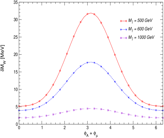
Figure 10: Squark contributions to $\delta M_{W}$ as function of the phase $(\phi_{A}+\phi_{\mu})$, where $\phi_{A}\equiv\phi_{A_{t}}=\phi_{A_{b}}$, for different values of the common sfermion mass $M_{\tilde{f}}=500$, $600$, $1000$ GeV. The other relevant SUSY parameters are set to $\tan\beta=5$, $|A_{t,b}|=2M_{\tilde{f}}$, $|\mu|=900$ GeV.

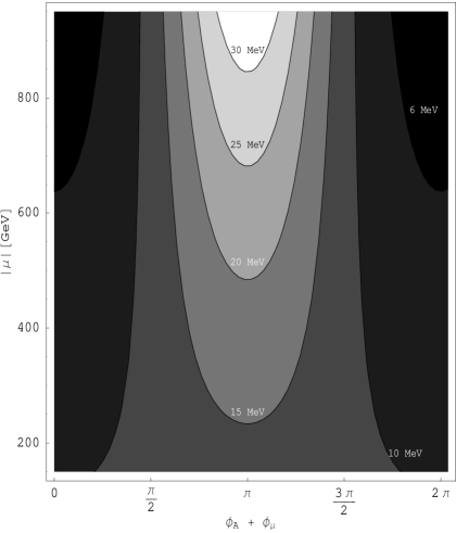
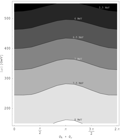
Figure 11: Contour lines of the squark contributions to $\delta M_{W}$ in the plane of $(\phi_{A}+\phi_{\mu})$ and $|\mu|$, where $\phi_{A}\equiv\phi_{A_{t}}=\phi_{A_{b}}$. The left plot shows a scenario with $\tan\beta=5$, $M_{\tilde{f}}=500\,\,\mathrm{GeV}$, $|A_{t,b}|=1000\,\,\mathrm{GeV}$, while in the right plot $\tan\beta=30$, $M_{\tilde{f}}=600\,\,\mathrm{GeV}$, $|A_{t,b}|=1200\,\,\mathrm{GeV}$.

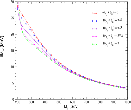
Figure 12: Squark contributions to $\delta M_{W}$ as function of a common sfermion mass $M_{\tilde{f}}$ for different values of $(\phi_{A_{t}}+\phi_{\mu})$. The other relevant SUSY parameters are: $|A_{t,b}|=350\,\,\mathrm{GeV}$, $(\phi_{A_{b}}+\phi_{\mu})=0$, $|\mu|=300\,\,\mathrm{GeV}$ and $\tan\beta=10$.

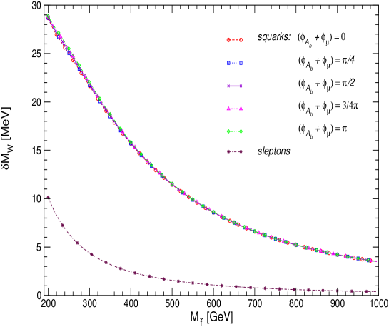
Figure 13: Squark and slepton contributions to $\delta M_{W}$ as function of a common sfermion mass $M_{\tilde{f}}$ for different values of $(\phi_{A_{b}}+\phi_{\mu})$. The other relevant SUSY parameters are: $|A_{t,b}|=350\,\,\mathrm{GeV}$, $(\phi_{A_{t}}+\phi_{\mu})=0$, $|\mu|=300\,\,\mathrm{GeV}$ and $\tan\beta=10$.

In the following plots we discuss the dependence of the sfermion loop contributions to $\delta M_{W}$ on the common sfermion mass $M_{\tilde{f}}$. In Fig. 12 we show the squark contributions as function of $M_{\tilde{f}}$ for various values of $(\phi_{A_{t}}+\phi_{\mu})$ and for $(\phi_{A_{b}}+\phi_{\mu})=0$. The intermediate value $\tan\beta=10$ is chosen, and $|A_{t,b}|=350\,\,\mathrm{GeV}$, $|\mu|=300\,\,\mathrm{GeV}$. In agreement with the discussion above, the phase dependence is relatively small. It leads to a shift of about $5$ MeV in $M_{W}$ for low values of $M_{\tilde{f}}\approx 250$ GeV, where the stop mixing is large. The total squark contributions can shift the prediction of $M_{W}$ by up to 30 MeV for small $M_{\tilde{f}}$. For large $M_{\tilde{f}}$ the squark contributions show the expected decoupling behaviour. However, even for sfermion masses as large as $M_{\tilde{f}}=1000$ GeV the shift in $M_{W}$ is still about $4$ MeV, i.e. half the size of the anticipated GigaZ accuracy.

In Fig. 13 we show the squark and slepton contributions for the same parameters as before except that $(\phi_{A_{t}}+\phi_{\mu})=0$ and $(\phi_{A_{b}}+\phi_{\mu})$ is varied. The effect of the phase $(\phi_{A_{b}}+\phi_{\mu})$ in the squark contributions is negligible since the sbottom mixing is small and moreover $|X_{b}|\approx|\mu|\tan\beta$, making its phase dependence insignificant. The slepton contributions (entering via the diagrams in Fig. 2) yield a shift in $M_{W}$ of up to 10 MeV for small $M_{\tilde{f}}$, i.e. about a third of the squark contributions. Even for the slepton contributions the dominant effect (about 60% of the total shift in $M_{W}$) can be associated with $\Delta\rho$, as a consequence of the D-term splitting of the sleptons. For large $M_{\tilde{f}}$ the slepton contributions show the expected decoupling behaviour.

4.1.2 Chargino and neutralino sector dependence

In this subsection we analyse the one-loop contributions from neutralinos and charginos to $\delta M_{W}$, entering via the self-energy, vertex and box diagrams shown in Figs. 6 and 7. In this sector the parameters $M_{1}$, $M_{2}$ and $\mu$ can be complex. However, there are only two physical complex phases since one of the two phases of $M_{1}$ and $M_{2}$ can be rotated away. As commonly done we choose to rotate away the phase of $M_{2}$. Generally, the phase dependence in this sector can be expected to be smaller than in the sfermion sector since the chargino/neutralino mass matrices are dominated by their diagonal elements, and the mass eigenvalues are mainly determined by $|\mu|$, $|M_{1,2}|$, so that their phase dependence is small.

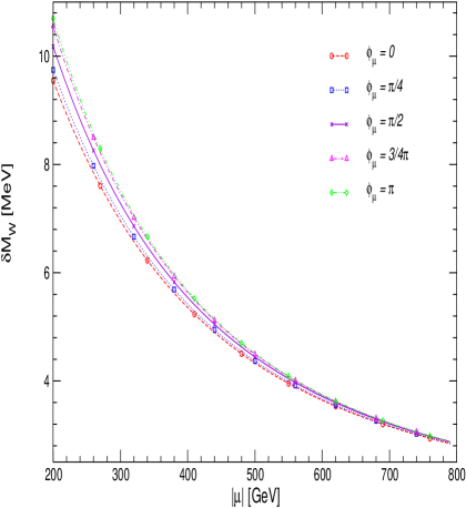
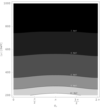
Figure 14: Neutralino and chargino contributions to $\delta M_{W}$. The left plot shows $\delta M_{W}$ as function of $|\mu|$ for different values of $\phi_{\mu}$, while the right plot displays the contour lines of $\delta M_{W}$ in the $\phi_{\mu}$–$|\mu|$ plane. The other relevant SUSY parameters are: $\phi_{M_{1}}=\phi_{M_{2}}=0$, $|M_{1}|=|M_{2}|=200\,\,\mathrm{GeV}$, $\tan\beta=10$ and $M_{\tilde{f}}=500\,\,\mathrm{GeV}$.

The phase dependence is illustrated by Fig. 14, where the chargino/neutralino contributions to $M_{W}$ are shown as function of $|\mu|$ (left panel) and as contour lines in the $\phi_{\mu}$–$|\mu|$ plane (right panel) for $\phi_{M_{1}}=0$. The other parameters are $M_{\tilde{f}}=500\,\,\mathrm{GeV}$, $M_{1}=M_{2}=200\,\,\mathrm{GeV}$ and $\tan\beta=10$. The effect of varying $\phi_{\mu}$ is much smaller than the overall contribution of the chargino/neutralino sector. In the scenario of Fig. 14 the chargino/neutralino contributions lead to a shift in the prediction for $M_{W}$ of up to $11\,\,\mathrm{MeV}$ for small $|\mu|$, while the effect of varying $\phi_{\mu}$ does not exceed $1\,\,\mathrm{MeV}$. We have checked that also the dependence on $\phi_{M_{1}}$ is insignificant.

In Fig. 15 we investigate the impact of varying $|M_{1}|$ and $|M_{2}|$ for zero complex phases. The other relevant parameters are $M_{\tilde{f}}=250\,\,\mathrm{GeV}$, $|\mu|=300\,\,\mathrm{GeV}$, $\tan\beta=10$. The shift in $M_{W}$ induced by varying $|M_{2}|$ can reach up to $15\,\,\mathrm{MeV}$ (i.e. the anticipated LHC precision). This is larger than the maximum shift in Fig. 14 because of the smaller sfermion masses. On the other hand, the effect of varying $|M_{1}|$ stays below $\sim 2\,\,\mathrm{MeV}$.

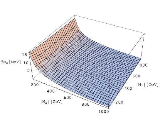
Figure 15: Neutralino and chargino contributions to $\delta M_{W}$ as function of $|M_{1}|$ and $|M_{2}|$. The other relevant SUSY parameters are: $\phi_{M_{1}}=\phi_{M_{2}}=\phi_{\mu}=0$, $|\mu|=300\,\,\mathrm{GeV}$, $\tan\beta=10$ and $M_{\tilde{f}}=250\,\,\mathrm{GeV}$.

4.1.3 Gauge boson and Higgs sector dependence

Finally we discuss the one-loop effects on $M_{W}$ from the gauge and Higgs sectors. In order to identify the genuine SUSY effects, we compare the contribution in the MSSM with the one in the SM (where the Higgs-boson mass in the SM is set equal to the mass of the light ${\cal CP}$-even Higgs boson of the MSSM, $M_{H^{\mathrm{SM}}}=M_{h}^{\rm MSSM}$). The corresponding diagrams are shown in Figs. 3, 4 and 5, where only the diagrams shown in Fig. 4 differ in the MSSM and the SM. The parameters governing the Higgs sector at the tree level are $M_{A}$ and $\tan\beta$ in the MSSM and $M_{H^{\mathrm{SM}}}$ in the SM. Since we incorporate higher-order contributions into the predictions for the MSSM Higgs masses and mixing angles, which are evaluated using the program FeynHiggs, further SUSY parameters enter the prediction for the gauge-boson and Higgs sector contribution. The effect of complex phases entering via the MSSM Higgs sector is formally of two-loop order. We therefore restrict to real parameters in this subsection.

In Fig. 16 the shift $\delta M_{W}$ is given as a function of $M_{A}$ in the MSSM and in the SM (with $M_{H^{\mathrm{SM}}}=M_{h}^{\rm MSSM}$). The parameter $\tan\beta$ is fixed to $\tan\beta=5,25$, which affects $M_{h}^{\rm MSSM}$ and accordingly also $M_{H^{\mathrm{SM}}}$. The other SUSY parameters are chosen as $M_{\tilde{f}}=600\,\,\mathrm{GeV}$, $A_{t,b}=1200\,\,\mathrm{GeV}$, $\mu=500\,\,\mathrm{GeV}$, $m_{\tilde{g}}=500\,\,\mathrm{GeV}$, $M_{2}=500\,\,\mathrm{GeV}$. Fig. 16 shows that the overall effect of the gauge and Higgs boson sector is rather large, up to $-60\,\,\mathrm{MeV}$, which corresponds to about twice the current experimental error on $M_{W}$. The shift in the $W$ boson mass obtained in the MSSM is slightly larger than in the SM. However, this genuine SUSY effect, i.e. the difference between the MSSM and the SM value of $\delta M_{W}$, is always below $\sim 2\,\,\mathrm{MeV}$ for $\tan\beta=5$ and smaller than $\sim 5\,\,\mathrm{MeV}$ for $\tan\beta=25$. The genuine SUSY effect is therefore below the anticipated GigaZ accuracy.

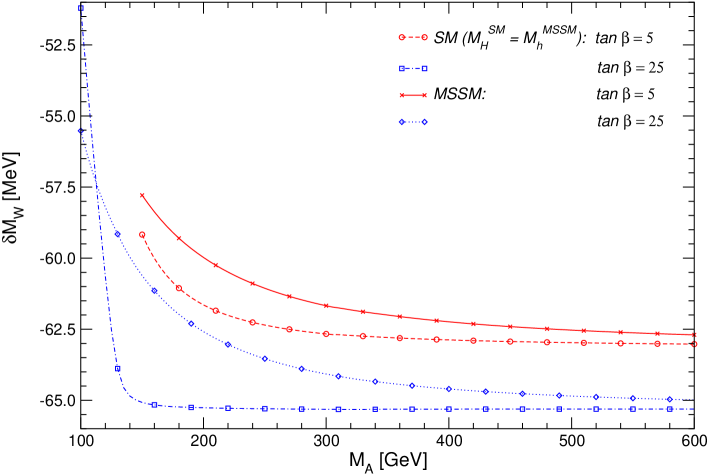
Figure 16: The contribution $\delta M_{W}$ to the prediction for the $W$ boson mass from the gauge-boson and Higgs sector contributions in the MSSM and the SM, where the SM contributions are evaluated for $M_{H^{\mathrm{SM}}}=M_{h}^{\rm MSSM}$. The shift $\delta M_{W}$ is given as a function of the ${\cal CP}$-odd Higgs-boson mass $M_{A}$ and $\tan\beta=5,25$. The other SUSY parameters were chosen to be: $M_{\tilde{f}}=600\,\,\mathrm{GeV}$, $A_{t,b}=1200\,\,\mathrm{GeV}$, $\mu=500\,\,\mathrm{GeV}$, $m_{\tilde{g}}=500\,\,\mathrm{GeV}$, $M_{2}=500\,\,\mathrm{GeV}$.

4.2 Prediction for $M_{W}$

In this section we combine all known contributions as described in Sect. 3.2 and analyse the parameter dependence of this currently most accurate MSSM prediction for $M_{W}$ in various scenarios. These predictions are compared with the current experimental value for $M_{W}$ [2],

$$M_{W}^{\rm exp}=80.404\pm 0.030\,\,\mathrm{GeV}~{}.$$ (42)

4.2.1 Dependence on SUSY parameters

We start by comparing our full MSSM prediction for $M_{W}$ with the corresponding SM value (with $M_{H^{\mathrm{SM}}}=M_{h}$) as a function of $M_{A}$ in Fig. 17. Like in Fig. 16 the other parameters are $M_{\tilde{f}}=600\,\,\mathrm{GeV}$, $A_{t,b}=1200\,\,\mathrm{GeV}$, $\mu=500\,\,\mathrm{GeV}$, $m_{\tilde{g}}=500\,\,\mathrm{GeV}$, $M_{2}=500\,\,\mathrm{GeV}$. $\tan\beta$ is set to $\tan\beta=5,25$. It can be seen in Fig. 17 that for this set of parameters the MSSM prediction is about $20\,\,\mathrm{MeV}$ higher than the SM prediction. While the MSSM prediction is within $1\sigma$ of the experimental value of $M_{W}$, the SM prediction lies in the 1–$2\sigma$ interval.

Figure 17: Prediction for $M_{W}$ in the MSSM and the SM, where the SM contributions are evaluated for $M_{H^{\mathrm{SM}}}=M_{h}^{\rm MSSM}$. The prediction for $M_{W}$ is shown as function of the ${\cal CP}$-odd Higgs-boson mass $M_{A}$ for $\tan\beta=5,25$. The other SUSY parameters are: $M_{\tilde{f}}=600\,\,\mathrm{GeV}$, $A_{t,b}=2\,M_{\tilde{f}}$, $\mu=500\,\,\mathrm{GeV}$, $m_{\tilde{g}}=500\,\,\mathrm{GeV}$, $M_{2}=500\,\,\mathrm{GeV}$.

In Fig. 18 we show the prediction for $M_{W}$ as a function of $M_{\tilde{f}}$ and indicate how this prediction changes if the top-quark mass is varied within its experimental $1\sigma$ interval, $m_{t}=(172.5\pm 2.3)\,\,\mathrm{GeV}$ [58]. The other parameters are $A_{t,b}=2\,M_{\tilde{f}}$, $\mu=M_{A}=m_{\tilde{g}}=M_{2}=300\,\,\mathrm{GeV}$, and $\tan\beta=10$. The result is compared with the current experimental value of $M_{W}$. It can be seen in Fig. 18 that the observable $M_{W}$ exhibits a slight preference for a relatively low SUSY scale, see also Refs. [5, 6] for a recent discussion of this issue. For the current experimental central value of the top-quark mass, $M_{W}$ lies in the experimental $1\sigma$-interval only for a SUSY mass scale of $M_{\tilde{f}}\;\raisebox{-3.00003pt}{$\stackrel{{\scriptstyle\displaystyle<}}{{\sim}}$}\;800\,\,\mathrm{GeV}$. Increasing $m_{t}$ by one standard deviation allows $M_{\tilde{f}}$ up to at least $1300\,\,\mathrm{GeV}$ at the $1\sigma$ level for this set of SUSY parameters.

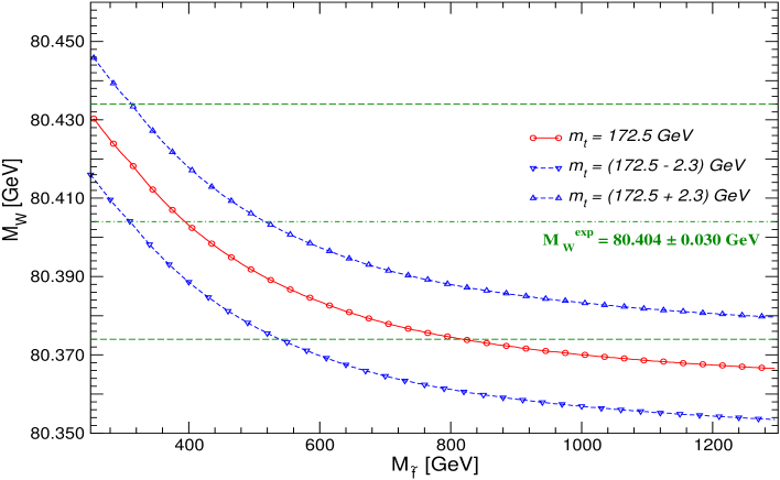
Figure 18: Prediction for $M_{W}$ as function of a common sfermion mass for $m_{t}=(172.5\pm 2.3)\,\,\mathrm{GeV}$. The other SUSY parameters are set to be: $A_{t,b}=2\,M_{\tilde{f}}$, $\tan\beta=10$, $\mu=300\,\,\mathrm{GeV}$, $m_{\tilde{g}}=300\,\,\mathrm{GeV}$, $M_{A}=300\,\,\mathrm{GeV}$, $M_{2}=300\,\,\mathrm{GeV}$.

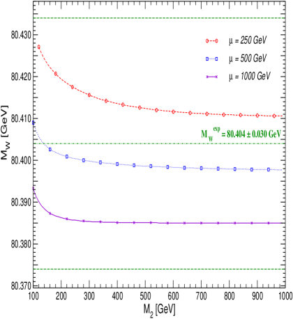
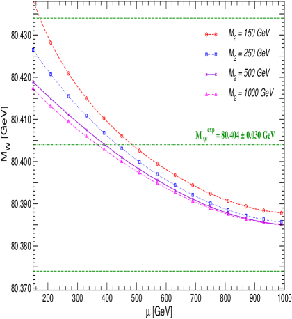
Figure 19: Prediction for $M_{W}$ as function of $M_{2}$ for $\mu=250\,\,\mathrm{GeV},\,500\,\,\mathrm{GeV},\,1000\,\,\mathrm{GeV}$ (left plot) and as function of $\mu$ for $M_{2}=150\,\,\mathrm{GeV},\,250\,\,\mathrm{GeV},\,500\,\,\mathrm{GeV},\,1000\,\,\mathrm{GeV}$ (right plot). The other SUSY parameters are: $M_{\tilde{f}}=300\,\,\mathrm{GeV}$, $A_{t,b}=2\,M_{\tilde{f}}$, $\tan\beta=10$, $m_{\tilde{g}}=600\,\,\mathrm{GeV}$, $M_{A}=1000\,\,\mathrm{GeV}$.

In Fig. 19 we show the dependence of $M_{W}$ on $\mu$ and $M_{2}$. The other parameters are set to $M_{\tilde{f}}=300\,\,\mathrm{GeV}$, $A_{t,b}=2\,M_{\tilde{f}}$, $M_{A}=1000\,\,\mathrm{GeV}$, $m_{\tilde{g}}=600\,\,\mathrm{GeV}$, $\tan\beta=10$. As can be seen in Fig. 19, varying $\mu$ between about $200\,\,\mathrm{GeV}$ and $1000\,\,\mathrm{GeV}$ results in a downward shift of more than $40\,\,\mathrm{MeV}$ in $M_{W}$. This strong dependence on the $\mu$ parameter is due to the neutralino and chargino as well as the squark contributions (one- and two-loop) to $\Delta r$. The sensitivity to the $\mu$ parameter from both MSSM particle sectors adds up and leads to the large shifts shown in Fig. 19. The neutralino and chargino contributions are responsible for roughly one third of the $40\,\,\mathrm{MeV}$ shift for small $M_{2}$ and become negligible for large $M_{2}$, with the remaining MSSM parameters specified as given above. The shift induced by varying $M_{2}$ between about $100\,\,\mathrm{GeV}$ and $1000\,\,\mathrm{GeV}$ (as explained above, $M_{2}$ and $M_{1}$ are varied simultaneously according to eq. (37)) amounts up to about $15\,\,\mathrm{MeV}$ in $M_{W}$. For the relatively small value chosen for the common sfermion mass, $M_{\tilde{f}}=300\,\,\mathrm{GeV}$, all combinations of $\mu$ and $M_{2}$ yield a result within $1\sigma$ of the experimental result of $M_{W}$. Using instead a larger SUSY mass scale of, for instance, $M_{\tilde{f}}=600\,\,\mathrm{GeV}$ would result in $M_{W}$ values within the experimental $1\sigma$ interval only for $\mu\;\raisebox{-3.00003pt}{$\stackrel{{\scriptstyle\displaystyle<}}{{\sim}}$}\;500\,\,\mathrm{GeV}$.

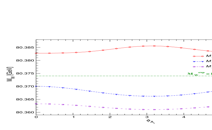
Figure 20: Prediction for $M_{W}$ as a function of the phase of $A_{t}$ using relation (32). The SUSY parameters are $|A_{t,b}|=1000\,\,\mathrm{GeV}$, $\phi_{A_{b}}=0$, $\tan\beta=10$, $m_{\tilde{g}}=500\,\,\mathrm{GeV}$, $M_{A}=500\,\,\mathrm{GeV}$, $M_{2}=250\,\,\mathrm{GeV}$ and $\mu=500\,\,\mathrm{GeV}$.

Finally we discuss the effect of varying the complex phase $\phi_{A_{t}}$ on the prediction for $M_{W}$. As explained above, we use our complete one-loop result for the phase dependence and employ eq. (32) to approximate the effect of the complex phases at the two-loop level. In Fig. 20 the prediction for $M_{W}$ is shown as a function of $\phi_{A_{t}}$ for $|A_{t,b}|=1000\,\,\mathrm{GeV}$, $\phi_{A_{b}}=0$, $\tan\beta=10$, $m_{\tilde{g}}=500\,\,\mathrm{GeV}$, $M_{A}=500\,\,\mathrm{GeV}$, $M_{2}=250\,\,\mathrm{GeV}$ and $\mu=500\,\,\mathrm{GeV}$. The results are plotted for $M_{\tilde{f}}=500\,\,\mathrm{GeV},600\,\,\mathrm{GeV}$ and $1000\,\,\mathrm{GeV}$. The dependence on $\phi_{A_{t}}$ is at most of the order $2\,\,\mathrm{MeV}$ for $M_{\tilde{f}}=500\,\,\mathrm{GeV},600\,\,\mathrm{GeV}$. For heavier sfermions with $M_{\tilde{f}}=1000\,\,\mathrm{GeV}$ only a $1\,\,\mathrm{MeV}$ shift in $M_{W}$ can be observed.

As explained above, our result for $M_{W}$ goes beyond the results previously known in the literature [3] because of the inclusion of complex phases and an improved treatment of higher-order SM contributions. We have checked that for real parameters our new result agrees with the previously most advanced implementation [3] typically within about $5\,\,\mathrm{MeV}$.

4.2.2 The SPS inspired benchmark scenarios

In this subsection we show $M_{W}$ in the SPS 1a, SPS 1b and SPS 5 benchmark scenarios [34]. This should give an indication of the $M_{W}$ prediction within “typical” constrained MSSM (CMSSM) scenarios. In the original definition the SPS parameters are $\overline{\rm{DR}}$ parameters. Here we treat them as on-shell input parameters for simplicity, since the effects of the $\overline{\rm{DR}}$ to on-shell transition are expected to be small and therefore irrelevant for the qualitative features that we discuss. In order to analyse the dependence of $M_{W}$ on the scale of supersymmetry we introduce a scale factor. Every SUSY parameter of mass dimension of the considered SPS point is multiplied by this parameter, i.e. $M_{A}=(\textup{scalefactor})\times M_{A}^{\textup{SPS}}$, $M_{{\tilde{F}},{\tilde{F}^{\prime}}}=(\textup{scalefactor})\times M_{{\tilde{F}},{\tilde{F}^{\prime}}}^{\textup{SPS}}$, $A_{t,b}=(\textup{scalefactor})\times A_{t,b}^{\textup{SPS}}$, $\mu=(\textup{scalefactor})\times\mu^{\textup{SPS}}$, $M_{1,2,3}=(\textup{scalefactor})\times M_{1,2,3}^{\textup{SPS}}$.

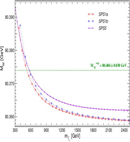
Figure 21: Prediction for $M_{W}$ within the SPS 1a, SPS 1b and SPS 5 inspired scenarios. $M_{W}$ is shown as a function of $m_{\tilde{t}_{1}}$, the lighter of the two stop squarks (left plot), and as a function of $M_{A}$, the mass of the ${\cal CP}$-odd Higgs boson (right plot). The SPS parameters of mass dimension are varied with the scale of supersymmetry as described in the text.

In Fig. 21 we show the result for the three SPS scenarios as a function of the lighter $\tilde{t}$ mass, $m_{\tilde{t}_{1}}$ (left plot), and as a function of $M_{A}$ (right plot). The prediction for $M_{W}$ is similar in all three scenarios. The variation of the dimensionful SUSY parameters shifts the MSSM prediction for $M_{W}$ by up to $35\,\,\mathrm{MeV}$. As can be seen in the left plot of Fig. 21, agreement at the $1\sigma$ level with the experimental result is obtained for $m_{\tilde{t}_{1}}\;\raisebox{-3.00003pt}{$\stackrel{{\scriptstyle\displaystyle<}}{{\sim}}$}\;600\,\,\mathrm{GeV}$. Since we scale all dimensionful parameters simultaneously, the variation from small to large $m_{\tilde{t}_{1}}$ (left plot) is the same as the one from small to large $M_{A}$ (right plot). However, for the same $M_{A}$ value the three scenarios can differ also by up to $\sim 30\,\,\mathrm{MeV}$.

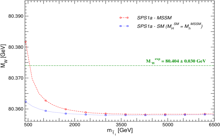
Figure 22: Prediction for $M_{W}$ in the decoupling limit compared to the SM prediction with $M_{H^{\mathrm{SM}}}=M_{h}^{\rm MSSM}$. $M_{W}$ is shown as function of the light stop mass $m_{\tilde{t}_{1}}$ in the SPS 1a benchmark scenario. All dimensionful SUSY parameters are scaled with a common factor, as described in the text.

For large values of the SUSY mass scale one expects a decoupling behaviour of the SUSY contributions, i.e. one expects that the prediction for $M_{W}$ in the MSSM coincides with the SM prediction (for $M_{H^{\mathrm{SM}}}=M_{h}^{\rm MSSM}$) in the limit of large SUSY masses. We analyse the decoupling behaviour in Fig. 22 for the SPS 1a scenario. We compare the MSSM prediction with the corresponding SM prediction of $M_{W}$ with $M_{H^{\mathrm{SM}}}=M_{h}^{\rm MSSM}$. For $m_{\tilde{t}_{1}}\;\raisebox{-3.00003pt}{$\stackrel{{\scriptstyle\displaystyle<}}{{\sim}}$}\;500\,\,\mathrm{GeV}$ large deviations between the MSSM and the SM prediction can be observed. For $m_{\tilde{t}_{1}}\;\raisebox{-3.00003pt}{$\stackrel{{\scriptstyle\displaystyle>}}{{\sim}}$}\;2500\,\,\mathrm{GeV}$ the difference drops below the level of $1\,\,\mathrm{MeV}$, and for even larger $m_{\tilde{t}_{1}}$ values the MSSM result converges to the SM result. It should be noted in this context that the prescription described in Sect. 3.2.1 (see eq. (29)) has been crucial in order to recover the most up-to-date SM prediction for $M_{W}$ in the decoupling limit.

4.2.3 The focus point scenario

As we have seen in the previous section, a relatively light SUSY scale leads to a prediction for $M_{W}$ within the CMSSM (and of course also the unconstrained MSSM) that is in slightly better agreement with the experimental value of $M_{W}$ than the SM prediction. A region of the CMSSM that has found a considerable interest in the last years is the so-called focus point region [67]. This region is characterized by a relatively small fermionic mass parameter, $m_{1/2}$, while the common scalar mass parameter $m_{0}$ is very large, and also $\tan\beta$ is relatively large. We now investigate whether it is also possible to obtain a prediction for $M_{W}$ that is in better agreement with the experimental value than the SM prediction if the MSSM parameters are restricted to the focus point region.

We have evaluated three representative scenarios, using $m_{t}=172.5\,\,\mathrm{GeV}$, $\tan\beta=50$ and $\mu>0$. We have chosen a point with the currently lowest value of $m_{1/2}$ in the focus point region for which the dark matter density is allowed by WMAP and other cosmological data (see e.g. Ref. [6] for a more detailed discussion) and two further points with higher $m_{1/2}$ (and higher $m_{0}$) along the strip in the $m_{1/2}$–$m_{0}$ plane that is allowed by the dark matter constraints. These points yield the following results for $M_{W}$ in the MSSM

$$(1) m_{1/2}=250\,\,\mathrm{GeV},m_{0}=1650\,\,\mathrm{GeV},A_{0}=-250\,\,\mathrm{GeV}$$ (45)

$$\Rightarrow M_{W}=80.380\,\,\mathrm{GeV},\ \ \ \ \ \ M_{W}^{\rm SM}(M_{H^{\mathrm{SM}}}=M_{h}^{\rm MSSM})=80.361\,\,\mathrm{GeV},$$

$$(2) m_{1/2}=330\,\,\mathrm{GeV},m_{0}=2030\,\,\mathrm{GeV},A_{0}=-330\,\,\mathrm{GeV}$$

$$\Rightarrow M_{W}=80.372\,\,\mathrm{GeV},\ \ \ \ \ \ M_{W}^{\rm SM}(M_{H^{\mathrm{SM}}}=M_{h}^{\rm MSSM})=80.360\,\,\mathrm{GeV},$$

$$(3) m_{1/2}=800\,\,\mathrm{GeV},m_{0}=3685\,\,\mathrm{GeV},A_{0}=-800\,\,\mathrm{GeV}$$

$$\Rightarrow M_{W}=80.361\,\,\mathrm{GeV},\ \ \ \ \ \ M_{W}^{\rm SM}(M_{H^{\mathrm{SM}}}=M_{h}^{\rm MSSM})=80.359\,\,\mathrm{GeV},$$

where the low-scale parameters of the MSSM have been obtained from the high-scale parameters $m_{1/2}$, $m_{0}$, $A_{0}$ with the help of the program ISAJET 7.71 [68]. For comparison, the corresponding prediction in the SM with $M_{H^{\mathrm{SM}}}=M_{h}^{\rm MSSM}$ is also given.

One can see from eqs. (45)–(45) that only for the point with the lowest $m_{1/2}$ value a large difference of up to $\sim 20\,\,\mathrm{MeV}$ occurs in comparison to the SM result. Such low $m_{1/2}$ values correspond to very low masses of neutralinos and charginos. As a consequence, the main contribution to the shift in $M_{W}$ arises from the chargino and neutralino sector (see Sect. 4.1.2). Since for the $m_{0}$ value of eq. (45) the squarks are not completely decoupled, there is also a small contribution from the squark sector. Already with slightly higher $m_{1/2}$ values, eq. (45), the contribution to $M_{W}$ becomes much smaller. For even higher values, eq. (45), the resulting prediction for $M_{W}$ is very close to the corresponding SM (decoupling) limit. These predictions deviate by about $1.5\sigma$ from the current experimental value of $M_{W}$, eq. (42). The focus point region therefore improves the prediction for $M_{W}$ only for very low $m_{1/2}$. For most of the allowed parameter space, however, the improvement is small. The deviation in $M_{W}$ contributes to the relatively bad fit quality of the focus point region in a fit to electroweak precision observables as observed in Ref. [6].

4.2.4 Split SUSY

Another scenario that has recently found attention is the so-called “split-SUSY” scenario [69]. Here scalar mass parameters are made very heavy and only the fermionic masses (i.e. the chargino, neutralino and gluino masses) are relatively small. According to the analysis in the previous sections only a small deviation in the $M_{W}$ prediction from the SM limit is to be expected.

We have evaluated the prediction for $M_{W}$ in the split-SUSY scenario. In Fig. 23 we show the SUSY contribution to $M_{W}$, i.e. the deviation between the MSSM result in the split-SUSY scenario and the corresponding SM result. This deviation is obtained by choosing a large value for $M_{\tilde{f}}$ and subtracting the SM result with $M_{H^{\mathrm{SM}}}=M_{h}^{\rm MSSM}$. For definiteness we have chosen $M_{\tilde{f}}=3\,\,\mathrm{TeV}$ and $M_{A}=2\,\,\mathrm{TeV}$. Choosing a higher scale for the scalar mass parameters would lead to even slightly smaller deviations from the SM prediction than the ones shown in Fig. 23. The resulting shifts in $M_{W}$ are displayed in Fig. 23 in the $\mu$–$M_{2}$ plane for $\tan\beta=10$. The gluino mass has been set to $m_{\tilde{g}}=300\,\,\mathrm{GeV}$, however no visible change in Fig. 23 occurs even for $m_{\tilde{g}}=3000\,\,\mathrm{GeV}$. As expected, only for rather small values of $\mu$ and $M_{2}$, $M_{2}\;\raisebox{-3.00003pt}{$\stackrel{{\scriptstyle\displaystyle<}}{{\sim}}$}\;400\,\,\mathrm{GeV}$ and $|\mu|\;\raisebox{-3.00003pt}{$\stackrel{{\scriptstyle\displaystyle<}}{{\sim}}$}\;500\,\,\mathrm{GeV}$ a deviation from the SM limit larger than $5\,\,\mathrm{MeV}$ is found (a similar result has been obtained in Ref. [70], see also Ref. [71]). Even with the GigaZ precision for $M_{W}$ only a very light chargino/neutralino spectrum would result in a $1\sigma$ deviation in $M_{W}$ compared to the SM prediction.

Figure 23: Difference between the result for $M_{W}$ in the MSSM and the SM for large scalar fermion masses. The SUSY parameters are $M_{\tilde{f}}=3000\,\,\mathrm{GeV}$, $A_{t,b}=2\,M_{\tilde{f}}$, $m_{\tilde{g}}=300\,\,\mathrm{GeV}$, $M_{A}=2000\,\,\mathrm{GeV}$ and $\tan\beta=10$.

4.2.5 MSSM parameter scans

Finally, we analyse the overall behaviour of $M_{W}$ in the MSSM by scanning over a broad range of the SUSY parameter space. The following SUSY parameters are varied independently of each other, within the given range, in a random parameter scan:

$${\rm sleptons} : M_{{\tilde{F}},{\tilde{F}^{\prime}}}=100\dots 2000\,\,\mathrm{GeV}$$

$${\rm light~{}squarks} : M_{{\tilde{F}},{\tilde{F}^{\prime}}_{\textup{up/down}}}=100\dots 2000\,\,\mathrm{GeV}$$

$$\tilde{t}/\tilde{b}{\rm~{}doublet} : M_{{\tilde{F}},{\tilde{F}^{\prime}}_{\textup{up/down}}}=100\dots 2000\,\,\mathrm{GeV}$$

$$A_{t,b}=-2000\dots 2000\,\,\mathrm{GeV}$$

$${\rm gauginos} : M_{1,2}=100\dots 2000\,\,\mathrm{GeV}$$

$$m_{\tilde{g}}=195\dots 1500\,\,\mathrm{GeV}$$

$$\mu=-2000\dots 2000\,\,\mathrm{GeV}$$

$${\rm Higgs} : M_{A}=90-1000\,\,\mathrm{GeV}$$ (46)

$$\tan\beta=1.1\dots 60$$

We have taken into account the constraints on the MSSM parameter space from the LEP Higgs searches [72, 73] and the lower bounds on the SUSY particle masses from Ref. [35]. Apart from these constraints no other restrictions on the MSSM parameter space were made.

In Fig. 24 we show the result for $M_{W}$ as a function of the lightest $\tilde{t}$ mass, $m_{\tilde{t}_{1}}$. The top-quark mass has been fixed to its current experimental central value, $m_{t}=172.5\,\,\mathrm{GeV}$. The results are divided into a dark (green) shaded and a light (green) shaded area. In the latter at least one of the ratios $m_{\tilde{t}_{2}}/m_{\tilde{t}_{1}}$ or $m_{\tilde{b}_{2}}/m_{\tilde{b}_{1}}$ exceeds 2.5, i.e. the darker shaded region corresponds to a moderate splitting among the $\tilde{t}$ or $\tilde{b}$ doublets. In this region the MSSM prediction for $M_{W}$ does not exceed values of about $80.550\,\,\mathrm{GeV}$. In the case of very large splitting in the $\tilde{t}$ and $\tilde{b}$ doublets, much larger $M_{W}$ values up to $81.150\,\,\mathrm{GeV}$ would be possible (which are of course ruled out by the experimental measurement of $M_{W}$).

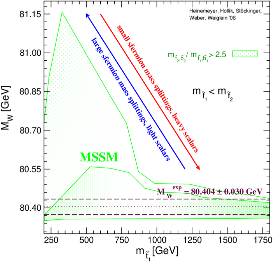
\begin{picture}(0.0,0.0) \put(0.0,0.0){} \put(0.0,0.0){} \end{picture}

Figure 24: Prediction for $M_{W}$ as function of $m_{\tilde{t}_{1}}$, the mass of the lighter stop squark. The SUSY parameters are varied independently of each other in a random parameter scan as described in the text. The top-quark mass is fixed at its current experimental central value, $m_{t}=172.5\,\,\mathrm{GeV}$.

In Fig. 25 we compare the SM and the MSSM predictions for $M_{W}$ as a function of $m_{t}$ as obtained from the scatter data. The predictions within the two models give rise to two bands in the $m_{t}$–$M_{W}$ plane with only a relatively small overlap region (indicated by a dark-shaded (blue) area in Fig. 25). The allowed parameter region in the SM (the medium-shaded (red) and dark-shaded (blue) bands) arises from varying the only free parameter of the model, the mass of the SM Higgs boson, from $M_{H^{\mathrm{SM}}}=114\,\,\mathrm{GeV}$, the LEP exclusion bound [73] (upper edge of the dark-shaded (blue) area), to $400\,\,\mathrm{GeV}$ (lower edge of the medium-shaded (red) area). The very light-shaded (green), the light shaded (green) and the dark-shaded (blue) areas indicate allowed regions for the unconstrained MSSM. In the very light-shaded region (see Fig. 24) at least one of the ratios $m_{\tilde{t}_{2}}/m_{\tilde{t}_{1}}$ or $m_{\tilde{b}_{2}}/m_{\tilde{b}_{1}}$ exceeds 2.5, while the decoupling limit with SUSY masses of ${\cal O}(2\,\,\mathrm{TeV})$ yields the lower edge of the dark-shaded (blue) area. Thus, the overlap region between the predictions of the two models corresponds in the SM to the region where the Higgs boson is light, i.e. in the MSSM allowed region ($M_{h}\;\raisebox{-3.00003pt}{$\stackrel{{\scriptstyle\displaystyle<}}{{\sim}}$}\;135\,\,\mathrm{GeV}$ [38, 39]). In the MSSM it corresponds to the case where all superpartners are heavy, i.e. the decoupling region of the MSSM. The current 68% C.L. experimental results for $m_{t}$ and $M_{W}$ are indicated in the plot. As can be seen from Fig. 25, the current experimental 68% C.L. region for $m_{t}$ and $M_{W}$ exhibit a slight preference of the MSSM over the SM. The prospective accuracies for the Tevatron/LHC ($\delta m_{t}^{\rm Tevatron/LHC}=1\,\,\mathrm{GeV}$, $\delta M_{W}^{\rm Tevatron/LHC}=15\,\,\mathrm{MeV}$) and the ILC with GigaZ option ($\delta m_{t}^{\rm ILC/GigaZ}=0.1\,\,\mathrm{GeV}$, $\delta M_{W}^{\rm ILC/GigaZ}=7\,\,\mathrm{MeV}$) are also shown in the plot (using the current central values), indicating the potential for a significant improvement of the sensitivity of the electroweak precision tests [74].

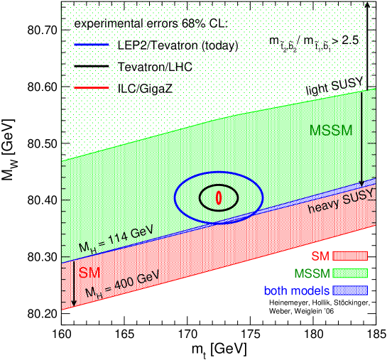
\begin{picture}(0.0,0.0) \put(0.0,0.0){} \put(0.0,0.0){} \end{picture}

Figure 25: Prediction for $M_{W}$ in the MSSM and the SM as a function of $m_{t}$ in comparison with the present experimental results for $M_{W}$ and $m_{t}$ and the prospective accuracies (using the current central values) at the Tevatron / LHC and at the ILC. The allowed region in the MSSM, corresponding to the light-shaded (green) and dark-shaded (blue) bands, results from varying the SUSY parameters independently of each other in a random parameter scan. The allowed region in the SM, corresponding to the medium-shaded (red) and dark-shaded (blue) bands, results from varying the mass of the SM Higgs boson from $M_{H}=114\,\,\mathrm{GeV}$ to $M_{H}=400\,\,\mathrm{GeV}$. Values in the very light shaded region can only be obtained in the MSSM if at least one of the ratios $m_{\tilde{t}_{2}}/m_{\tilde{t}_{1}}$ or $m_{\tilde{b}_{2}}/m_{\tilde{b}_{1}}$ exceeds 2.5.

4.3 Remaining higher-order uncertainties

As explained above, we have incorporated all known SM corrections into the prediction for $M_{W}$ in the MSSM, see eq. (29). This implies that the theoretical uncertainties from unknown higher-order corrections reduce to those in the SM in the decoupling limit. In the SM, based on all higher-order contributions that are currently known, the remaining uncertainty in $M_{W}$ has been estimated to be [16]

$$\delta M_{W}^{\rm SM}=4\,\,\mathrm{MeV}~{}.$$ (47)

Below the decoupling limit an additional theoretical uncertainty arises from higher-order corrections involving supersymmetric particles in the loops. This uncertainty has been estimated in Ref. [30] for the MSSM with real parameters depending on the overall sfermion mass scale $M_{\tilde{f}}$,

$$\delta M_{W} = 8.5\,\,\mathrm{MeV}\mbox{ for }M_{\tilde{f}}<500\,\,\mathrm{GeV},$$

$$\delta M_{W} = 2.7\,\,\mathrm{MeV}\mbox{ for }M_{\tilde{f}}=500\,\,\mathrm{GeV},$$ (48)

$$\delta M_{W} = 2.4\,\,\mathrm{MeV}\mbox{ for }M_{\tilde{f}}=1000\,\,\mathrm{GeV}.$$

The full theoretical uncertainty from unknown higher-order corrections in the MSSM with real parameters can be obtained by adding in quadrature the SM uncertainties from eq. (47) and the SUSY uncertainties from eq. (48). This yields $\delta M_{W}=(4.7\,-\,9.4)\,\,\mathrm{MeV}$ depending on the SUSY mass scale [30].

Allowing SUSY parameters to be complex adds an additional theoretical uncertainty from unknown higher-order corrections to the $M_{W}$ prediction. While at the one-loop level the full complex phase dependence is included in our evaluation, it is only approximately taken into account at the two-loop level as an interpolation between the known results for the phases 0 and $\pi$, see eq. (32). We concentrate here on the complex phase in the scalar top sector, $\phi_{A_{t}}$ (we keep $\phi_{\mu}$ fixed), since our analysis above has revealed that the impact of the other phases is very small already at the one-loop level.

We estimate the uncertainty from unknown higher-order corrections associated with the phase dependence as follows. The full result for $M_{W}(\phi)$, i.e. for a given phase $\phi$ (where the two-loop corrections are taken into account as described in Sect. 3.2.3) lies by construction in the interval

$$[M_{W}^{\rm full}(0)+(M_{W}^{1{\rm L}}(\phi)-M_{W}^{1{\rm L}}(0)),\quad M_{W}^{\rm full}(\pi)+(M_{W}^{1{\rm L}}(\phi)-M_{W}^{1{\rm L}}(\pi))]~{}.$$ (49)

The minimum difference of $M_{W}^{\rm full}(\phi)$ to the boundary of this interval,

$${\rm Min}\{|M_{W}^{\rm full}(\phi)-(M_{W}^{\rm full}(0)+(M_{W}^{1{\rm L}}(\phi)-M_{W}^{1{\rm L}}(0)))|,|M_{W}^{\rm full}(\phi)-(M_{W}^{\rm full}(\pi)+(M_{W}^{1{\rm L}}(\phi)-M_{W}^{1{\rm L}}(\pi)))|\}~{},$$ (50)

can be taken as estimate for the theoretical uncertainty (this automatically ensures that no additional uncertainties arise for $\phi=0,\pi$).

As representative SUSY scenarios we have chosen SPS 1a, SPS 1b, and SPS 5, each for $M_{\tilde{f}}=1000\,\,\mathrm{GeV}$, $500\,\,\mathrm{GeV}$, and for $M_{\tilde{f}}<500\,\,\mathrm{GeV}$  (as above we have varied $M_{\tilde{f}}$, $A_{t,b}$ and $\mu$ using a common scale factor). A non-zero complex phase $\phi_{A_{t}}$ has been introduced as an additional parameter. In order to arrive at a conservative estimate for the intrinsic error, we use the value obtained for $\phi_{A_{t}}=\pm\pi/2$. In this way we obtain

$$\delta M_{W} = 3.2\,\,\mathrm{MeV}\mbox{ for }M_{\tilde{f}}<500\,\,\mathrm{GeV},$$

$$\delta M_{W} = 2.0\,\,\mathrm{MeV}\mbox{ for }M_{\tilde{f}}=500\,\,\mathrm{GeV},$$ (51)

$$\delta M_{W} = 0.7\,\,\mathrm{MeV}\mbox{ for }M_{\tilde{f}}=1000\,\,\mathrm{GeV}.$$

The full theoretical uncertainty from unknown higher-order corrections in the MSSM with complex parameters can now be obtained by adding in quadrature the SM uncertainties from eq. (47), the theory uncertainties from eq. (48) and the additional SUSY uncertainties from eq. (51). This yields $\delta M_{W}=(4.7-9.9)\,\,\mathrm{MeV}$ depending on the SUSY mass scale.

The other source of theoretical uncertainties besides the one from unknown higher-order corrections is the parametric uncertainty induced by the experimental errors of the input parameters. The current experimental error of the top-quark mass [58] induces the following parametric uncertainty in $M_{W}$

$$\delta m_{t}^{\rm exp}=2.3\,\,\mathrm{GeV}\;\;\Rightarrow\;\;\delta M_{W}^{{\rm para},m_{t}}=14\,\,\mathrm{MeV}~{},$$ (52)

while the uncertainty in $\Delta\alpha_{\rm had}^{(5)}$ [75] results in

$$\delta(\Delta\alpha_{\rm had}^{(5)})=3.6\times 10^{-4}\;\;\Rightarrow\;\;\delta M_{W}^{{\rm para},\Delta\alpha_{\rm had}^{(5)}}=6.5\,\,\mathrm{MeV}~{}.$$ (53)

The uncertainty in $m_{t}$ will decrease during the next years as a consequence of a further improvement of the accuracies at the Tevatron and the LHC. Ultimately it will be reduced by more than an order of magnitude at the ILC [76]. For $\Delta\alpha_{\rm had}^{(5)}$ one can hope for an improvement down to $5\times 10^{-5}$ [77], reducing the parametric uncertainty to the $1\,\,\mathrm{MeV}$ level (for a discussion of the parametric uncertainties induced by the other SM input parameters see e.g. Ref. [3]). The effect of $\delta(\Delta\alpha_{\rm had}^{(5)})$ on Fig. 25 is small. In order to reduce the theoretical uncertainties from unknown higher-order corrections to the $1\,\,\mathrm{MeV}$ level, further results on SM-type corrections beyond two-loop order and higher-order corrections involving supersymmetric particles will be necessary.

5 Conclusions

We have presented the currently most accurate evaluation of the $W$ boson mass in the MSSM. The calculation includes the complete one-loop result, taking into account for the first time the full complex phase dependence, and all known higher-order corrections in the MSSM. Since the evaluation of higher-order contributions in the SM is more advanced than in the MSSM, we have incorporated all available SM corrections which go beyond the results obtained so far in the MSSM. Our prediction for $M_{W}$ in the MSSM therefore reproduces the currently most up-to-date SM prediction for $M_{W}$ in the decoupling limit where the masses of all supersymmetric particles are large. A public computer code based on our result for $M_{W}$ is in preparation.

We have analysed in detail the impact of the various sectors of the MSSM on the prediction for $M_{W}$, focussing in particular on the dependence on the complex phases entering at the one-loop level. The most pronounced phase dependence occurs in the stop sector, where the effect of varying the complex phase that enters the off-diagonal element in the stop mass matrix can amount to a shift of more than 20 MeV in $M_{W}$. It should be noted, however, that the complex phases in the squark sector at the one-loop level enter only via modifications of the squark masses and mixing angles. As a consequence, a precision measurement of the ${\cal CP}$-conserving observable $M_{W}$ alone will not be sufficient to reveal the presence of ${\cal CP}$-violating complex phases. The phase dependence of $M_{W}$ will however be very valuable for constraining the SUSY parameter space in global fits where all accessible experimental information is taken into account.

We have illustrated the sensitivity of the precision observable $M_{W}$ to indirect effects of new physics by comparing our MSSM prediction with the SM case. Confronting the MSSM prediction in different SUSY scenarios and the SM result as a function of the Higgs-boson mass with the current experimental values of $M_{W}$ and $m_{t}$, we find a slight preference for non-zero SUSY contributions. As representative SUSY scenarios we have studied various SPS benchmark points, where we have varied all mass parameters using a common scalefactor. The MSSM prediction lies within the $1\sigma$ region of the experimental $M_{W}$ value if the SUSY mass scale is relatively light, i.e. lower than about 600 GeV.

The prospective improvement in the experimental accuracy of $M_{W}$ at the next generation of colliders will further enhance the sensitivity to loop contributions of new physics. We have found that even for a SUSY mass scale of several hundred GeV the loop contribution of supersymmetric particles to $M_{W}$ is still about 10 MeV, which may be probed in the high-precision environment of the ILC. In SUSY scenarios with even higher mass scales, however, it is unlikely that SUSY loop contributions to $M_{W}$ can be resolved with the currently foreseen future experimental accuracies. We have studied in this context the focus point and the split-SUSY scenarios, which have recently received significant attention in the literature. In the focus point scenario only at the lower edge of the allowed parameter region in the $m_{1/2}$–$m_{0}$ plane a sizeable contribution to $M_{W}$ can be achieved. For higher values, as well as for the split-SUSY scenario, we find that the SUSY loop effects are in general very small, so that it is not possible to bring the prediction for $M_{W}$ significantly closer to the current experimental central value as compared to the SM case.

Finally we have analysed the theoretical uncertainties in the $M_{W}$ prediction that arise from the incomplete inclusion of the complex phases at the two-loop level. We estimate that this uncertainty can amount up to roughly $3\,\,\mathrm{MeV}$ in the prediction for $M_{W}$, depending on the SUSY mass scale. Combined with the estimate of the possible effects of other unknown higher-order corrections we find that the total uncertainty from unknown higher-order contributions is currently about $10\,\,\mathrm{MeV}$ for small SUSY mass scales.

Acknowledgements

We are grateful to T. Hahn for many helpful discussions on various aspects of this work. S.H. and G.W. thank the Max Planck Institut für Physik, München, for kind hospitality during part of this work.

References

-
[1]
[The ALEPH, DELPHI, L3, OPAL, SLD Collaborations,
the LEP Electroweak Working Group,
the SLD Electroweak and Heavy Flavour Groups],
hep-ex/0509008;
[The ALEPH, DELPHI, L3 and OPAL Collaborations, the LEP Electroweak Working Group], hep-ex/0511027. -
[2]
F. Spano,
talk given at Rencontres de Moriond,
Electroweak Interactions and Unified Theories,
La Thuile, Italy, March 2006,
see also:
lepewwg.web.cern.ch/LEPEWWG/Welcome.html. - [3] S. Heinemeyer, W. Hollik and G. Weiglein, Phys. Rept. 425 (2006) 265, hep-ph/0412214.
-
[4]
H. Nilles,
Phys. Rept. 110 (1984) 1;
H. Haber and G. Kane, Phys. Rept. 117 (1985) 75;
R. Barbieri, Riv. Nuovo Cim. 11 (1988) 1. - [5] J. Ellis, S. Heinemeyer, K. Olive and G. Weiglein, JHEP 0502 013, hep-ph/0411216; hep-ph/0508169.
- [6] J. Ellis, S. Heinemeyer, K. Olive and G. Weiglein, JHEP 0605 (2006) 005, hep-ph/0602220.
- [7] The CDF and D0 Experiments, see: www-cdf.fnal.gov/physics/projections/ .
- [8] S. Haywood et al., hep-ph/0003275, in: Standard Model Physics (and more) at the LHC, eds. G. Altarelli and M. Mangano, CERN, Geneva, 1999 [CERN-2000-004].
- [9] G. Wilson, LC-PHSM-2001-009, see: www.desy.de/lcnotes/notes.html .
- [10] U. Baur, R. Clare, J. Erler, S. Heinemeyer, D. Wackeroth, G. Weiglein and D. Wood, hep-ph/0111314.
-
[11]
A. Sirlin,
Phys. Rev. D 22 (1980) 971;
W. Marciano and A. Sirlin, Phys. Rev. D 22 (1980) 2695. -
[12]
A. Freitas, W. Hollik, W. Walter and G. Weiglein,
Phys. Lett. B 495 (2000) 338
[Erratum-ibid. B 570 (2003) 260],
hep-ph/0007091;
Nucl. Phys. B 632 (2002) 189
[Erratum-ibid. B 666 (2003) 305],
hep-ph/0202131;
M. Awramik and M. Czakon, Phys. Lett. B 568 (2003) 48, hep-ph/0305248. -
[13]
M. Awramik and M. Czakon,
Phys. Rev. Lett. 89 (2002) 241801,
hep-ph/0208113;
Nucl. Phys. Proc. Suppl. 116 (2003) 238,
hep-ph/0211041;
A. Onishchenko and O. Veretin, Phys. Lett. B 551 (2003) 111, hep-ph/0209010;
M. Awramik, M. Czakon, A. Onishchenko and O. Veretin, Phys. Rev. D 68 (2003) 053004, hep-ph/0209084. -
[14]
A. Djouadi and C. Verzegnassi,
Phys. Lett. B 195 (1987) 265;
A. Djouadi, Nuovo Cim. A 100 (1988) 357. -
[15]
B. Kniehl,
Nucl. Phys. B 347 (1990) 89;
F. Halzen and B. Kniehl, Nucl. Phys. B 353 (1991) 567;
B. Kniehl and A. Sirlin, Nucl. Phys. B 371 (1992) 141; Phys. Rev. D 47 (1993) 883;
A. Djouadi and P. Gambino, Phys. Rev. D 49 (1994) 3499 [Erratum-ibid. D 53 (1994) 4111], hep-ph/9309298. - [16] M. Awramik, M. Czakon, A. Freitas and G. Weiglein, Phys. Rev. D 69 (2004) 053006, hep-ph/0311148.
-
[17]
L. Avdeev et al.,
Phys. Lett. B 336 (1994) 560
[Erratum-ibid. B 349 (1995) 597],
hep-ph/9406363;
K. Chetyrkin, J. Kühn and M. Steinhauser, Phys. Lett. B 351 (1995) 331, hep-ph/9502291; Nucl. Phys. B 482 (1996) 213, hep-ph/9606230. - [18] K. Chetyrkin, J. Kühn and M. Steinhauser, Phys. Rev. Lett. 75 (1995) 3394, hep-ph/9504413.
- [19] J. van der Bij, K. Chetyrkin, M. Faisst, G. Jikia and T. Seidensticker, Phys. Lett. B 498 (2001) 156, hep-ph/0011373.
- [20] M. Faisst, J. Kühn, T. Seidensticker and O. Veretin, Nucl. Phys. B 665 (2003) 649, hep-ph/0302275.
- [21] R. Boughezal, J. Tausk and J. van der Bij, Nucl. Phys. B 713 (2005) 278, hep-ph/0410216.
-
[22]
R. Barbieri and L. Maiani,
Nucl. Phys. B 224 (1983) 32;
C. Lim, T. Inami and N. Sakai, Phys. Rev. D 29 (1984) 1488;
E. Eliasson, Phys. Lett. B 147 (1984) 65;
Z. Hioki, Prog. Theo. Phys. 73 (1985) 1283;
J. Grifols and J. Solà, Nucl. Phys. B 253 (1985) 47;
B. Lynn, M. Peskin and R. Stuart, CERN Report 86-02, p. 90;
R. Barbieri, M. Frigeni, F. Giuliani and H. Haber, Nucl. Phys. B 341 (1990) 309;
M. Drees and K. Hagiwara, Phys. Rev. D 42 (1990) 1709. - [23] M. Drees, K. Hagiwara and A. Yamada, Phys. Rev. D 45 (1992) 1725.
- [24] P. Chankowski, A. Dabelstein, W. Hollik, W. Mösle, S. Pokorski and J. Rosiek, Nucl.Phys. B 417 (1994) 101.
- [25] D. Garcia and J. Sola, Mod.Phys.Lett. A9 (1994) 211.
- [26] D. Pierce, J. Bagger, K. Matchev and R. Zhang, Nucl. Phys. B 491 (1997) 3, hep-ph/9606211.
- [27] S. Kang and J. Kim, Phys. Rev. D 62 (2000) 071901, hep-ph/0008073.
- [28] A. Djouadi, P. Gambino, S. Heinemeyer, W. Hollik, C. Jünger and G. Weiglein, Phys. Rev. Lett. 78 (1997) 3626, hep-ph/9612363; Phys. Rev. D 57 (1998) 4179, hep-ph/9710438.
-
[29]
S. Heinemeyer,
PhD Thesis, Univ. Karlsruhe, Shaker Verlag, Aachen 1998,
ISBN 3826537874,
see www-itp.physik.uni-karlsruhe.de/prep/phd/;
G. Weiglein, hep-ph/9901317. - [30] J. Haestier, S. Heinemeyer, D. Stöckinger and G. Weiglein, JHEP 0512 (2005) 027, hep-ph/0508139; hep-ph/0506259.
- [31] S. Heinemeyer and G. Weiglein, JHEP 0210 (2002) 072, hep-ph/0209305; hep-ph/0301062.
- [32] S. Heinemeyer, W. Hollik, F. Merz, S. Peñaranda, Eur. Phys. J. C 37 (2004) 481, hep-ph/0403228.
- [33] J. Aguilar-Saavedra et al., Eur. Phys. J. C 46 (2006) 43, hep-ph/0511344.
-
[34]
B. Allanach et al.,
Eur. Phys. J. C 25 (2002) 113,
hep-ph/0202233;
The definition of the MSSM parameter for the SPS points can be found at
www.ippp.dur.ac.uk/georg/sps/ . - [35] S. Eidelman et al. [Particle Data Group Collaboration], Phys. Lett. B 592 (2004) 1.
-
[36]
R. Behrends, R. Finkelstein and A. Sirlin,
Phys. Rev. 101 (1956) 866;
S. Berman, Phys. Rev. 112 (1958) 267;
T. Kinoshita and A. Sirlin, Phys. Rev. 113 (1959) 1652. -
[37]
T. van Ritbergen and R. Stuart,
Phys. Rev. Lett. 82 (1999) 488,
hep-ph/9808283;
Nucl. Phys. B 564 (2000) 343,
hep-ph/9904240;
M. Steinhauser and T. Seidensticker, Phys. Lett. B 467 (1999) 271, hep-ph/9909436. - [38] S. Heinemeyer, W. Hollik and G. Weiglein, Comput. Phys. Comm. 124 2000 76, hep-ph/9812320; Eur. Phys. J. C 9 (1999) 343, hep-ph/9812472. The code is accessible via www.feynhiggs.de .
- [39] G. Degrassi, S. Heinemeyer, W. Hollik, P. Slavich and G. Weiglein, Eur. Phys. J. C 28 (2003) 133, hep-ph/0212020.
-
[40]
T. Hahn, S. Heinemeyer, W. Hollik and G. Weiglein,
hep-ph/0507009;
M. Frank, T. Hahn, S. Heinemeyer, W. Hollik, H. Rzehak and G. Weiglein, in preparation. - [41] S. Heinemeyer, W. Hollik, and G. Weiglein, Eur. Phys. J. C 16 (2000) 139, hep-ph/0003022.
- [42] S. Heinemeyer, W. Hollik, J. Rosiek, and G. Weiglein, Eur. Phys. J. C 19 (2001) 535, hep-ph/0102081.
- [43] M. Veltman, Nucl. Phys. B 123 (1977) 89.
-
[44]
G. ’t Hooft and M. Veltman,
Nucl. Phys. B 44 (1972) 189;
C. Bollini and J. Giambiagi, Nuovo Cimento B 12 (1972) 20;
J. Ashmore, Nuovo Cimento Lett. 4 (1972) 289. -
[45]
W. Siegel,
Phys. Lett. B 84 (1979) 193;
D. Capper, D. Jones and P. van Nieuwenhuizen, Nucl. Phys. B 167 (1980) 479;
W. Siegel, Phys. Lett. B 94 (1980) 37;
L. Avdeev, Phys. Lett. B 117 (1982) 317;
L. Avdeev and A. Vladimirov, Nucl. Phys. B 219 (1983) 262;
I. Jack and D. Jones, hep-ph/9707278, in Perspectives on Supersymmetry, ed. G. Kane (World Scientific, Singapore), p. 149;
D. Stöckinger, JHEP 0503 (2005) 076, hep-ph/0503129. -
[46]
J. Küblbeck, M. Böhm and A. Denner,
Comput. Phys. Comm. 60 (1990) 165;
T. Hahn, Nucl. Phys. Proc. Suppl. 89 (2000) 231, hep-ph/0005029; Comput. Phys. Comm. 140 (2001) 418, hep-ph/0012260.
The program is available via www.feynarts.de . - [47] T. Hahn and C. Schappacher, Comput. Phys. Comm. 143 (2002) 54, hep-ph/0105349.
-
[48]
G. Weiglein, R. Scharf and M. Böhm,
Nucl. Phys. B 416 (1994) 606,
hep-ph/9310358;
G. Weiglein, R. Mertig, R. Scharf and M. Böhm, in New Computing Techniques in Physics Research 2, ed. D. Perret-Gallix (World Scientific, Singapore, 1992), p. 617. - [49] T. Hahn and M. Pérez-Victoria, Comput. Phys. Comm. 118 (1999) 153, hep-ph/9807565; see: www.feynarts.de/formcalc .
-
[50]
G. Weiglein,
Acta Phys. Polon. B 29 (1998) 2735,
hep-ph/9807222;
A. Stremplat, Diploma Thesis (University of Karlsruhe, 1998). - [51] Y. Schröder and M. Steinhauser, Phys. Lett. B 622 (2005) 124, hep-ph/0504055.
-
[52]
R. Barbieri, M. Beccaria, P. Ciafaloni,
G. Curci and A. Vicere,
Nucl. Phys. B 409 (1993) 105;
J. Fleischer, F. Jegerlehner and O. Tarasov, Phys. Lett. B 319 (1993) 249. - [53] M. Consoli, W. Hollik and F. Jegerlehner, Phys. Lett. B 227(1989) 167.
- [54] A. M. Weber et al., in preparation
- [55] K. Hagiwara, A. Martin, D. Nomura and T. Teubner, Phys. Rev. D 69 (2004) 093003, hep-ph/0312250.
- [56] M. Steinhauser, Phys. Lett. B 429 (1998) 158, hep-ph/9803313.
- [57] J. Arguin et al. [The CDF Collaboration, the D0 Collaboration and the Tevatron Electroweak Working Group], hep-ex/0507091.
- [58] Tevatron Electroweak Working Group, hep-ex/0603039.
- [59] W. Hollik, J. Illana, S. Rigolin and D. Stöckinger, Phys. Lett. B 416 (1998) 345, hep-ph/9707437; Phys. Lett. B 425 (1998) 322, hep-ph/9711322.
- [60] D. Demir, O. Lebedev, K. Olive, M. Pospelov and A. Ritz, Nucl. Phys. B 680 (2004) 339, hep-ph/0311314.
-
[61]
D. Chang, W. Keung and A. Pilaftsis,
Phys. Rev. Lett. 82 (1999) 900
[Erratum-ibid. 83 (1999) 3972],
hep-ph/9811202;
A. Pilaftsis, Phys. Lett. B 471 (1999) 174, hep-ph/9909485. - [62] O. Lebedev, K. Olive, M. Pospelov and A. Ritz, Phys. Rev. D 70 (2004) 016003, hep-ph/0402023.
-
[63]
P. Nath,
Phys. Rev. Lett. 66 (1991) 2565;
Y. Kizukuri and N. Oshimo, Phys. Rev. D 46 (1992) 3025. -
[64]
T. Ibrahim and P. Nath,
Phys. Lett. B 418 (1998) 98,
hep-ph/9707409;
Phys. Rev. D 57 (1998) 478
[Erratum-ibid. D 58 (1998) 019901]
[Erratum-ibid. D 60 (1998) 079903]
[Erratum-ibid. D 60 (1999) 119901],
hep-ph/9708456;
M. Brhlik, G. Good and G. Kane, Phys. Rev. D 59 (1999) 115004, hep-ph/9810457. - [65] S. Abel, S. Khalil and O. Lebedev, Nucl. Phys. B 606 (2001) 151, hep-ph/0103320.
- [66] V. Barger, T. Falk, T. Han, J. Jiang, T. Li and T. Plehn, Phys. Rev. D 64 (2001) 056007, hep-ph/0101106.
-
[67]
J. Feng, K. Matchev and T. Moroi,
Phys. Rev. Lett. 84 (2000) 2322,
hep-ph/9908309;
Phys. Rev. D 61 (2000) 075005,
hep-ph/9909334;
J. Feng, K. Matchev and F. Wilczek, Phys. Lett. B 482 (2000) 388, hep-ph/0004043;
J. Feng and K. Matchev, Phys. Rev. D 63 (2001) 095003, hep-ph/0011356. - [68] F. Paige, S. Protopopescu, H. Baer and X. Tata, hep-ph/0312045.
-
[69]
N. Arkani-Hamed and S. Dimopoulos,
JHEP 0506 (2005) 073,
hep-th/0405159;
G. Giudice and A. Romanino, Nucl. Phys. B 699 (2004) 65 [Erratum-ibid. B 706 (2005) 65], hep-ph/0406088. - [70] J. Guasch and S. Peñaranda, JHEP 0601 (2006) 121, hep-ph/0508241.
- [71] S. Martin, K. Tobe and J. Wells, Phys. Rev. D 71 (2005) 073014, hep-ph/0412424.
- [72] [ALEPH, DELPHI, L3, OPAL Collaborations and LEP Working Group for Higgs boson searches], hep-ex/0602042.
- [73] G. Abbiendi et al. [ALEPH, DELPHI, L3, OPAL Collaborations and LEP Working Group for Higgs boson searches], Phys. Lett. B 565 (2003) 61, hep-ex/0306033.
-
[74]
S. Heinemeyer, T. Mannel and G. Weiglein,
hep-ph/9909538;
J. Erler, S. Heinemeyer, W. Hollik, G. Weiglein and P. Zerwas, Phys. Lett. B 486 (2000) 125, hep-ph/0005024;
J. Erler and S. Heinemeyer, hep-ph/0102083. - [75] H. Burkhardt and B. Pietrzyk, Phys. Rev. D 72 (2005) 057501, hep-ph/0506323.
- [76] S. Heinemeyer, S. Kraml, W. Porod and G. Weiglein, JHEP 0309 (2003) 075, hep-ph/0306181.
-
[77]
F. Jegerlehner,
talk presented at the LNF Spring School,
Frascati, Italy, 1999, see:
www.ifh.de/fjeger/Frascati99.ps.gz ; hep-ph/0105283.