A Simple Parameterization of the Cosmic-Ray Muon Momentum Spectra at the Surface as a Function of Zenith Angle

Abstract

The designs of many neutrino experiments rely on calculations of the background rates arising from cosmic-ray muons at shallow depths. Understanding the angular dependence of low momentum cosmic-ray muons at the surface is necessary for these calculations. Heuristically, from examination of the data, a simple parameterization is proposed, based on a straighforward scaling variable. This in turn, allows a universal calculation of the differential muon intensity at the surface for all zenith angles and essentially all momenta.

1 Introduction

There is a need among the experimental design community for the ability to accurately predict backgrounds from cosmic ray muons at relatively shallow depths – less than a few hundreds of meters of water equivalent (m.w.e.). In the past, most studies have focused on muon fluxes and intensities at very deep sites (greater than 1 km.w.e.) which do not accurately predict the behavior of muons below a few hundred GeV. Since shallow sites are dominated by muons between 3–20 GeV, the characteristic distributions of these muons can have a great impact on the designs of experimental laboratories and shielding geometries.

The momentum distribution of the vertical muon intensity ($I_{\textrm{v}}(p_{\mu})$ [cm${}^{-2}\cdot$ sr${}^{-1}\cdot$ s${}^{-1}\cdot$ GeV^-1]) at the surface is fairly well known, as many experiments have provided measurements. However, when calculating the total rate of muons for a given shielding configuration, it is the interplay between the angular distribution of muons as a function of momentum and the angular distribution of shielding and overburden which is important. While it is generally accepted[1] that the muon angular distribution is $\propto\cos^{2}\theta$ for low muon momenta of around 3 GeV, and that at higher momenta ($p_{\mu}>$ 100–200 GeV) it approaches a $\sec\theta$ distribution (for $\theta<70^{\circ}$), there is currently no simple way to accurately estimate the muon momentum spectra over all angles.

In this work, experimental data in which muon momentum distributions have been recorded at various zenith angles have been compared. A simple relationship has been found, $I(p_{\mu},\theta)=\cos^{3}(\theta)I_{\textrm{v}}(p_{\mu}\cos\theta)$ (cf. Fig. 3). It relates all angles to the differential vertical muon intensity distribution $I_{\textrm{v}}$ by simply scaling the independant variable (momentum) by $\cos\theta$ and the dependant variable ($I$) by $\cos^{3}\theta$. The theoretical interpretation of this intriguing universality remains unclear. An improved fit is provided which should allow surface muon intensity predictions over all zenith angles for the momentum range of most relevance to shallow sites: $p_{\mu}>1$GeV and $p_{\mu}<2000$GeV/$\cos\theta$.

2 Data Selection

Before analysing the data, some brief comments on the selection criteria are required. An attempt was made to include as much surface muon data at various zenith angles as possible. A majority of the available cosmic-ray muon data was recorded at underground locations. Since these data are usually reported after slant-depth corrections which inherently assume certain zenith angle dependancies, it was decided to exclude all data recorded at depth. Additionally, surface experiments for which the angular acceptance was not clearly specified or the systematic errors were not discussed were not included in this study.

The selected data, shown in Table 1, come from six surface muon experiments which measured intensity as a function of muon momentum and zenith angle. They span zenith angles from the vertical to the horizontal and cover muon momenta up to  2000 GeV/$\cos\theta$.

Table 1: The six experimental data sets that were included in this study. For each experiment, the ranges in energy and angular acceptance are shown for the individual data sets. When comparing data sets, the average value of $\cos(\theta)$ was used.

Experiment		Zenith Angle Range (∘)	$p_{\mu}$ (GeV)
Nandi and Sinha[2]	0∘	0 – 0.3	5 – 1200
MARS[3]	0∘	0 – 0.08	20 – 500
Kellogg et al.[4]	30∘	25.9 – 34.1	50 – 1700
	75∘	70.9 – 79.1	50 – 1700
OKAYAMA[5]	0∘	0 – 1	1.5 – 250
	30∘	26 – 34	2 – 250
	60∘	59 – 61	3 – 250
	75∘	69 – 81	3 – 250
	80∘	79 – 81	3 – 150
Kiel-Desy[6]	75∘	68 – 82	1 – 1000
MUTRON[7]	89∘	86 – 90	100 – 20,000

A few comments should be made about how the data are included here. Whenever a systematic error was listed, but not already included in the tabulated data, it was combined in quadrature with the statistical errors. The Kiel-Desy experiment reported differences between their measured differential spectra and the phenomenological fit used for correcting the data, primarily at low momenta (1–20 GeV). These differences were included as an additional systematic error.

For the Kellogg data, the angular acceptance of the magnetic spectrometer is listed as $\pm 11.4^{\circ}$. However, the efficiencies fall off rapidly and it is stated that the data are heavily peaked in the region of $\pm 4.1^{\circ}$ from the central zenith angle. For that reason, the lower angular range was used in this comparison.

There is some duplication in the OKAYAMA data set which should also be mentioned. The angular acceptance of the OKAYAMA telescope was $\pm 1^{\circ}$. The data at 30^∘ and 75^∘ were combined from smaller sets of zenith angle data to be more comparable to other data sets (e.g. those from Kellogg et al. or Kiel-Desy). As a result, the data at 80^∘ are a subset of the 75^∘ data set. It was felt, however, that including that data was still relevant to understanding the zenith angle dependence.

3 Data Comparison

In Fig. 1, the differential muon intensity data from all of the data sets listed in Table 1 are plotted together as a function of the muon momentum. One notes the power law dependence of the higher momentum data that can be approximated by $p_{\mu}^{-3.7}$. Attempts to describe the low momentum fall off and angular dependence as simple corrections to the primary power law have had minimal success.

However, a similarity in spectral shape can be seen between all the data sets (Fig. 2) if a simple scaling variable is introduced

$$\zeta=p_{\mu}\cos(\theta).$$ (1)

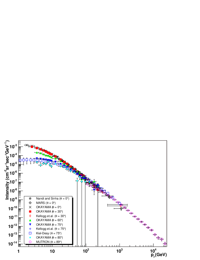
Figure 1: The differential surface muon intensity is plotted as a function of muon momentum for all the data sets listed in Table 1.

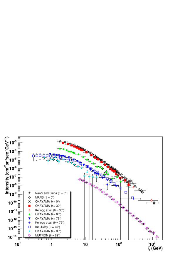
Figure 2: The differential surface muon intensity is plotted as a function of $\zeta$ as defined in Eq. 1. One clearly notices the similarity of spectral shape and the grouping of the different data by zenith angle.

Based on this observation, a succesful attempt was made to find a scale factor for all momenta $\propto 1/\cos^{n}(\theta)$. Optimal agreement was found at a value of $n=3$ (shown in Fig. 3).

This implies that a simple relationship exists in the data that relates the muon intensity at any momentum and angle to the vertical intensity ($I_{\textrm{v}}$) by

$$I(p_{\mu},\theta)=\cos^{3}(\theta)I_{\textrm{v}}(\zeta).$$ (2)

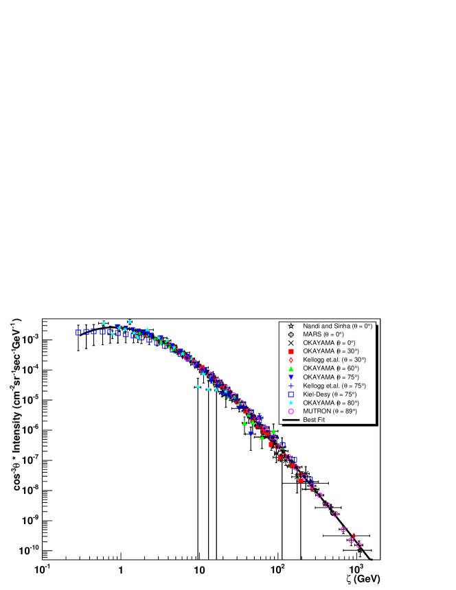
Figure 3: Surface muon intensity is plotted as a function of $\zeta=p_{\mu}\cos(\theta)$. Each data set is scaled by a factor $1/\cos^{3}(\theta)$. Also shown is the best fit, derived from combining Eqs. 2 and 3 as described in Section 4.

4 Comparison to Spectrum Models

As a side issue, this section discusses the specific form of $I$, and argues for the utility of the relationship expressed in Eq. 2. With the combined data, as shown in Fig. 3, it is possible to compare several parameterizations that attempt to provide calculations of muon intensity. Four such models are shown in Fig. 4.

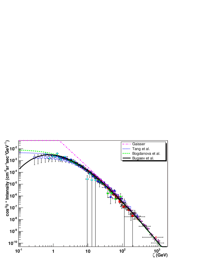
Figure 4: The combined date from Fig. 3 are compared to some parameterizations of vertical muon intensity (Gaisser[8] and Bugaev[11]) as well as some recent attempts at complete momentum and angle coverage in which the zenith angle was set to zero (Tang[10] and Bogdanova[9]).

The Gaisser[8] and Bugaev[11] models are both 5 parameter functions which describe only the vertical muon intensity while the other two models (Bogdanova[9] and Tang[10]) are recent attempts to better match the angular dependence of the intensity at the surface. The Gaisser formula is based on the physics of the muon production in the atmoshpere and was validated with most of the world’s data at depth. It is not expected to be valid at energies below the pion threshold ($\sim$100 GeV), but since it is a standard reference of the community, it is included here for comparison.

The Bugaev work is focused on nuclear cascade models for the propogation of high-energy nucleons, pions and kaon in the atmosphere. The formula provided is the result of a simple parameterization to thier calculations.

The work by Tang et al.[10] is an attempt to improve the initial Gaisser formula by including the effects due to the curvature of the earth to calculate the specific atmospheric path-length and density corrections for all zenith angles. In addition, an emperical functional modification is provided for $p_{\mu}<1$ GeV/$\cos\theta$ to improve compatibility with low energy data where muon decay is expected to be significant.

The Bogdanova model[9] is based on an optimization of the parameters in the emperical formula first proposed by Miyake[12]. It contains 3 simple terms which represent the muon production spectrum and the effects of pion and muon decay.

To evaluate the quality of these parameterizations, a $\chi^{2}$ comparison of each was performed to the entire data set (shown in Table 2).

Table 2: The $\chi^{2}$ comparison between the listed models and all the data shown in Table 1. In the last column, values of the intesity at all zenith angles are calculated by relying on the relationship in Eq. 2 and evaluating the given models for vertical intensity only. For the two models that provide an alternative zenith angle parameterization, this is compared in the “all $\theta$” column, which does not rely on Eq. 2.

Model	$\chi^{2}/n.d.f.$ (all $\theta$)	$\chi^{2}/n.d.f.$ (use Eq. 2)
Tang[10]	518.69 / 191	354.822 / 197
Bogdanova[9]	330.235 / 203	387.727 / 205
Bugaev[11]	–	232.861 / 204
Best Fit	–	165.62 / 204

Since the models of Bogdanova and Tang both provide zenith angular dependences, they were able to be compared to the data without the scaling relationship of Eq. 2 (shown in the column labeled “all $\theta$”).

However, when those same models were used for the vertical intensity only ($\theta$ is set to zero) and the relationship expressed in Eq. 2 was used to predict the angular dependance, the resulting $\chi^{2}$s are as good or better. Furthermore, the parameterization provided by Bugaev et al. provides an even better relation to the data, with a reduced $\chi^{2}$ approaching one.

An attempt was made to see if the inclusion of all of the data from the various zenith angles would allow for an improved solution of the coefficients in the Bugaev parameterization:

$$I_{\textrm{v}}(p_{\mu})=c_{1}p_{\mu}^{-1(c_{2}+c_{3}\log_{10}(p_{\mu})+c_{4}\log_{10}^{2}(p_{\mu})+c_{5}\log_{10}^{3}(p_{\mu})}.$$ (3)

The original coefficients were defined separately for 4 momentum ranges: 1 – 927.65 GeV, 927.65 – 1587.8 GeV, 1587.8 – 41625 GeV, and $>$41625 GeV.

Here, Eqs. 2 and 3 were combined and the values of the parameters were allowed to float. Fitting the entire sample of data, a $\chi^{2}$ of 165.6 for 204 degrees of freedom could be achieved (refered to as “Best Fit” in Table 2 and Fig. 3) – a modest improvement – by using the following coefficients:

$c_{1}$ = 0.00253

$c_{2}$ = 0.2455

$c_{3}$ = 1.288

$c_{4}$ = -0.2555

$c_{5}$ = 0.0209

Recall that this improved parameterization applies to all zenith angles. Given the available data, it can be considered valid for muon momenta $p_{\mu}>1$ GeV and $p_{\mu}<2000$ GeV/$\cos\theta$.

5 Conclusions

An examination of experimental data on muon intensities for various zenith angles at the surface has been performed. Within that data, a simple relationship has been found between the angular distribution and the vertical momentum spectrum of $I(p_{\mu},\theta)=\cos^{3}(\theta)I_{\textrm{v}}(\zeta)$ where $\zeta=p_{\mu}\cos(\theta)$. One wonders if it is perhaps significant that $\zeta$ is the component of the muon momentum perpendicular to the surface. Nevertheless, for the purpose of simulating muon intensities near the surface, this relation appears remarkably accurate.

The highest accuracy was achieved when using the functional form from [11] and adjusting the coefficients as described above (the result is labeled “Best Fit” in Table 2 and Fig. 3). For simulations in which energies of a few tens of GeV are important (less than 100 m.w.e.), it is recommended to use this modified fit. At greater depths, where the energies below 10 GeV can safely be neglected, the original parameters listed in [11] would probably be preferred, since they provide a smooth transition to higher values of $\zeta$. Although it was not studied in this work, it might be an interesting exercise to validate the angular correlation of Eq. 2 at higher energies.

References

- [1] S. Eidelman et al., Phys. Lett. B 592, 1 (2004).
- [2] B.C. Nandi and M.S. Sinha, J. Phys. A: Gen. Phys. 5, 1384 (1972).
- [3] C.A. Ayre, J.M. Baxendale, C.J. Hume, B.C. Nandi, M.G. Thompson and M.R. Whalley, J. Phys. G: Nucl. Phys. 1, 584 (1975).
- [4] R.G. Kellogg, H. Kasha and R.C. Larsen, Phys. Rev. D. 17, 98 (1978).
- [5] S. Tsuji, T. Katayama, K. Okei, T. Wada, I. Yamamoto and Y. Yamashita, J. Phys. G: Nucl. Phys. 24, 1805 (1998).
- [6] H. Jokisch, K. Carstensen, W.D. Dau, H.J. Meyer and O.C. Allkofer, Phys. Rev. D. 19, 1368 (1979).
- [7] S. Matsuno et al., Phys. Rev. D. 29, 1 (1984).
- [8] T. K. Gaisser, Cosmic Rays and Particle Physics. Cambridge, 1990.
- [9] L. N. Bogdanova, M. G. Gavrilov, V. N. Kornoukhov and A. S. Starostin, submitted to Phys. Atom. Nucl. [arXiv:nucl-ex/0601019].
- [10] A. Tang, G. Horton-Smith, V.A. Kudryavtsev and A. Tonazzo, submitted to Phys. Rev. E [arXiv:hep-ph/0604078].
- [11] E. V. Bugaev, A. Misaki, V. A. Naumov, T. S. Sinegovskaya, S. I. Sinegovsky and N. Takahashi, Phys. Rev. D 58, 054001 (1998) [arXiv:hep-ph/9803488].
- [12] S. Miyake, Proc. of the 13-th International Cosmic Ray Conference, Denver, Colorado Associated Univ. Press, Boulder (1973) Vol 5., p.3638.