HIP-2006-20/TH

Photon propagation in magnetic and electric fields with scalar/pseudoscalar couplings: a new look

Emidio Gabrielli^a, Katri Huitu^a,b, Sourov Roy^a

^aHelsinki Institute of Physics, P.O.B. 64, 00014 University of Helsinki, Finland
^bDiv. of HEP, Dept. of Physical Sciences, P.O.B. 64, 00014 University of Helsinki, Finland

We consider the minimal coupling of two photons to neutral scalar and pseudoscalar fields, as for instance in the case of the Higgs boson and axion, respectively. In this framework, we analyze the photon dispersion relations in the presence of static and homogeneous external magnetic and electric fields, by taking into account the contribution of the imaginary part of the scalar/pseudoscalar self-energy. We show that this contribution cannot be neglected when it is of the same order as the photon-scalar/pseudoscalar mixing term. In addition to the usual light-like photon propagation mode, with a refraction index $n>1$, a massive mode with mass of the order of the coupled boson mass can be induced, provided that the external field is above a particular critical value. Depending on the values of the external field, photon energy, and mass of the scalar/pseudoscalar particle, the scalar/pseudoscalar width could induce a sizeable rate of photon splitting in two photons due to a strong resonant phenomenon. This effect has no practical laboratory applications for the Higgs physics due to the very large critical external magnetic or electric fields involved, for a photon energy of the order of a TeV. However, it can have relevant consequences in the axion physics or in any other scenario where light neutral scalar/pseudoscalar fields have minimal coupling with two photons.

1 Introduction

Scalar and pseudoscalar neutral particles can have effective gauge invariant coupling with the electromagnetic field $A_{\mu}$ due to the higher dimensional operators. In particular, in the case of a scalar ($\varphi_{S}$) and pseudoscalar ($\varphi_{P}$) fields, the minimal interaction Lagrangians, proportional to the lowest dimensional gauge invariant operators, are given respectively by

$$L_{S} = -\frac{1}{4\Lambda_{S}}\,F_{\mu\nu}F^{\mu\nu}\,\varphi_{S}\,,$$ (1)

$$L_{P} = -\frac{1}{4\Lambda}_{P}\,F_{\mu\nu}\tilde{F}^{\mu\nu}\,\varphi_{P}\,,$$ (2)

where $F_{\mu\nu}=\partial_{\mu}A_{\nu}-\partial_{\nu}A_{\mu}$ is the electromagnetic field strength tensor, $\tilde{F}_{\mu\nu}=\frac{1}{2}\epsilon_{\mu\nu\alpha\beta}\,F^{\alpha\beta}$ its dual, and the mass scales $\Lambda_{S,P}$ parametrize the corresponding couplings.

Well known examples of such couplings to two photons can be found, for instance, in the framework of Higgs boson [1, 2] and axion physics [3, 4, 5]. The Higgs mechanism, responsible for the electroweak symmetry breaking (EWSB) in the Standard Model (SM), predicts a heavy scalar particle, the Higgs boson, which up to now has eluded any experimental test. The Higgs boson mass cannot be predicted in the framework of SM, and it ranges from the present experimental lower limit [6, 7] of 114 GeV, up to the theoretical upper bound of around $800$ GeV [1]. Although the Higgs boson has no tree-level coupling with two photons, it acquires such a coupling at 1-loop [2], with the corresponding scale $\Lambda_{S}$ of the order of ${\cal O}$(TeV).

On the contrary, the axion, which arises as a natural solution to the strong CP problem [3, 4], is a very light pseudoscalar particle which remains undetected due to the very weak coupling to ordinary matter. It appears as a pseudo Nambu-Goldstone boson of a spontaneously broken Peccei-Quinn symmetry [3] and has a mass $m_{A}$ expected to be of the order of $m_{A}\sim{\cal O}$(meV) [9, 10, 8, 11]. Moreover, since the corresponding coupling $\Lambda_{P}$ is of the order of $10^{10}-10^{11}$ GeV if astrophysical constraints are taken into account [11], the decay width of the axion into two photons, being proportional to $m_{A}^{3}/\Lambda_{P}^{2}$, is very small, implying that the axion is almost a stable particle on cosmic time scales.

The fact that a scalar field has an effective coupling with two photons, allows the $\gamma\to\varphi_{S}$ conversion mechanism in external magnetic or electric field to work by means of the Primakoff effect [12]. A simple way to look at this phenomenon is the following. By replacing one of the photon fields in $\varphi_{S}\gamma\gamma$ coupling in Eq.(1) with an external electromagnetic (EM) background field, the resulting $\varphi_{S}\gamma$ mixing term could be regarded as an off-diagonal term of the scalar-photon mass matrix, providing a source for the $\gamma\to\varphi_{S}$ transition. This is not in contradiction with angular momentum conservation, since due to the presence of the external field, the SO(3) rotational invariance for the total system radiation + background is restored. Analogous results hold for the pseudoscalar conversion mechanism $\gamma\to\varphi_{P}$ as well [9, 10].

The mechanism of photon-axion conversion in external magnetic field has been intensively studied in the literature [9, 10, 8, 11], especially in the context of astrophysics and cosmology [11], as the time evolution of the quantum system of two particle states. Due to the very large life-time of the axion, the photon-axion oscillation phenomenon is possible on macroscopic distances. However, it is worth stressing that the photon-axion conversion, with both fields on-shell, is not possible on strictly homogeneous and constant magnetic fields in all space. Indeed, due to the fact that the axion is a massive particle, the conservation of the energy and momentum at the axion-photon vertex requires inhomogeneity of the external magnetic field in order the reaction to proceed. Therefore, the transition amplitude comes out to be proportional to the form factor of the external field, inducing a suppression [9, 10, 8]. When the scale $(L)$ over which the magnetic field is homogeneous, is comparable or smaller than the scale of the inverse of the transfered momentum $\Delta P\sim m_{A}^{2}/(2E)$, the magnetic form factor could easily be of order ${\cal O}(1)$. This is indeed the case of optical photons and axion masses of the order of meV, where $\Delta PL\ll 1$. On the contrary, when $\Delta PL\gg 1$, a strong suppression is expected from the form factor if the magnetic field is homogeneous. However, the depletion induced by the form factor can be ameliorated by embedding the system in a plasma, and tuning the plasma frequency, which provides an effective mass for the photon, to be equal to the axion mass [13].

A particular class of experiments [14, 15] have been using the idea of the photon regeneration mechanism [9] in order to detect the axion in laboratory. After a Laser beam passes through a magnetic field, an axion component can be generated. The original incident Laser is then absorbed through a thick wall, but not the axion component. This can be then re-converted into photons by passing through a second magnet, the so-called phenomenon of light shining from a wall.

However, indirect effects of the axion coupling with two photons could give rise to the modification of photon dispersion relations in the presence of an external constant magnetic field [16]. In particular, these effects would induce the so called ‘Faraday rotation’, i.e. the rotation of the plane of polarization of a plane polarized light passing through a magnetic field [16]. The BFRT collaboration [15] has also performed a polarization experiment along these lines, but no significant deviation has been observed [14]. Recently, the PVLAS experiment [17], has reported the first evidence of a rotation of the polarization plane of light propagating through a static magnetic field. If confirmed, these results might point out the presence of a very light pseudoscalar particle weakly coupled to two photons. Alternative experiments have been proposed to check these results [19, 18]. The phenomenon of ‘Faraday rotation’ in a medium has also been analyzed in the context of QED [20].

In this framework, the aim of the present paper is to investigate the photon dispersion relations on static and homogeneous external electric or magnetic fields, by using the approach of the effective photon propagator. This last one is obtained after integrating out the scalar/pseudoscalar degree of freedom, or equivalently by summing up the relevant class of photon self-energy diagrams as done in our paper. Apart from the different approach, the new aspect with respect to previous studies mainly consists in the fact that we are including the contribution of scalar/pseudoscalar self-energy diagrams, where the effects of both real and imaginary parts are taken into account. In particular, we will show that the contribution of the imaginary part cannot be neglected. This approach would allow to analyze new phenomena not considered before, such as the effects of the scalar/pseudoscalar decay width ($\Gamma$) on the absorptive part of the effective photon propagator. Nevertheless, one should also expect that the width $\Gamma$ corrections could induce some effects on the rotation of the polarization plane of the incident photon, although we have not considered this aspect in the present work.

Analogous studies are well known in the framework of QED, where the refraction index for photon propagation and absorption coefficient have been determined in the case of photon propagating in strong magnetic fields [21, 22, 23]. In our case, this task can be easily achieved by summing up the full series of leading Feynman diagrams of photon self-energy and dispersion relations can then be derived by looking at the poles of the effective propagator. While the real part of the scalar/pseudoscalar self-energy (${\rm Re}\Sigma$) can be re-absorbed in the renormalization of the corresponding mass and wave function, the ${\rm Im}\Sigma$ would induce an imaginary part in the effective photon propagator, giving rise to a non-vanishing contribution to the photon absorption coefficient.

Due to the presence of the external field, the vacuum polarization and the dispersion relations will be modified with respect to the case without external sources. This will affect only the component of the photon polarization vector interacting with the external field, according to the Lagrangian in Eqs.(1), (2), while the other one will remain unaffected [16]. In particular, there will be two new propagation modes in addition to the one which is not modified. The lightest mode, corresponding to a light-like particle with a refraction index $n>1$, and a massive mode corresponding to a massive particle with mass of the order of the exchanged scalar/pseudoscalar one. By taking into account the effect of the scalar/pseudoscalar width $\Gamma$, we will show that the massive propagation mode is a solution of the dispersion relations only when the size of $\Gamma$ would be smaller or comparable to the effect of the mixing term, or in other words the massive solution is allowed only when the external magnetic or electric field is above some particular critical value.

Finally, we would like to stress that the scalar/pseudoscalar coupling with two photons can induce a sizeable contribution to the photon splitting process $\gamma\to\gamma\gamma$ in external magnetic or electric fields, depending on the magnitude of the external field and the photon energy involved. However, although suppressed by the corresponding width of the scalar or pseudoscalar field, the corresponding photon absorption coefficient may turn out to be significant due to a strong resonant phenomenon when the external field is in the vicinity of the critical value.

These results suggest a new class of experiments for searching indirect effects of the scalar/pseudoscalar coupling to two photons, like for instance by searching for the photon splitting $\gamma\to\gamma\gamma$ in constant magnetic fields. Notice that this process does not have any background since the analogous effect in QED is strongly suppressed for laboratory magnetic fields and photon energies in the optical or X-ray frequency range [21]. Therefore, any observation of photon splitting signal in laboratory would be a clear indication of new physics effects.

Returning to the scalar coupling with two photon, a well-known example in the standard model is provided by the Higgs boson [2]. Unfortunately, in this case a too large critical magnetic (or electric) external field would be required for photon energies of the order of TeV, with no practical laboratory applications. Nevertheless, we stress that sizeable effects on the photon absorption coefficient, induced by the Higgs boson, might be possible in astrophysical context, where sources of strong magnetic fields and/or very high energy photons can be found. For example in the core of a neutron star magnetic field can be as large as $10^{8}$ Tesla [5], although in that case plasma effects should be taken into account.

The plan of the paper is the following. In section 2, we present the results for the effective photon propagator in the presence of a static and homogeneous external magnetic field. In section 3, we provide the solutions to the photon dispersion relations, while in section 4 we will show the results of the photon absorption coefficient. In section 5 the phenomenological implications of these results will be analyzed and numerical results will be provided. Finally, in section 6 we will present our conclusions. In appendix A we report the exact solutions of the dispersion relations, while in appendix B we provide the calculation of the imaginary part of scalar(pseudoscalar) self-energy.

2 Effective photon propagator

Let us consider first the case of a scalar field and an external constant and homogeneous magnetic field $\vec{\rm B}$ assumed to be extended in all space. The Lagrangian containing the pure radiation field and other dynamical fields, can be obtained by decomposing the electromagnetic field strength $F_{\mu\nu}$ in two parts

$$F_{\mu\nu}=F_{\mu\nu}(A)+F_{\mu\nu}^{\rm(ext)}$$ (3)

where $F_{\mu\nu}(A)=\partial_{\mu}A_{\nu}-\partial_{\nu}A_{\mu}$ contains the usual photon radiation field $A_{\mu}$, while the $F_{\mu\nu}^{\rm(ext)}$ includes the corresponding term induced by the external magnetic field. After the shift in Eq.(3), the relevant Lagrangian would be given by

$$L=-\frac{1}{4}\,F_{\mu\nu}(A)F^{\mu\nu}(A)+\frac{1}{2}\partial_{\mu}\varphi_{S}\partial^{\mu}\varphi_{S}-\frac{1}{2}m^{2}\varphi_{S}^{2}-\frac{1}{4\Lambda_{S}}F_{\mu\nu}(A)F^{\mu\nu}(A)\varphi_{S}+L_{\rm ext}({\rm\vec{B}})$$ (4)

where $m$ is the mass of the scalar field and $L_{\rm ext}({\rm\vec{B}})$ is given by

$$L_{\rm ext}({\rm\vec{B}}) = -\frac{1}{4}F_{\mu\nu}^{\rm(ext)}F^{{\rm(ext)}\mu\nu}-\frac{1}{2}F_{\mu\nu}^{\rm(ext)}F^{\mu\nu}(A)-\frac{1}{2\Lambda_{S}}F^{\mu\nu}(A)F_{\mu\nu}^{\rm(ext)}\varphi_{S}$$ (5)

$$- \frac{1}{4\Lambda_{S}}F_{\mu\nu}^{\rm(ext)}F^{{\rm(ext)}\mu\nu}\varphi_{S}\,.$$

Notice that the last term in Eq.(5), in the case in which the external field is constant, is a tadpole term for the scalar field $\varphi_{S}$. It is easy to see that this tadpole has no physical effect since it can be eliminated by making the following constant shift $\varphi_{S}\to\varphi_{S}+\delta$ where $\delta=-F_{\mu\nu}^{\rm(ext)}F^{({\rm ext})\mu\nu}/(4\Lambda_{S}m^{2})$. The extra term $-\frac{\delta}{4\Lambda_{S}}F_{\mu\nu}(A)F^{\mu\nu}(A)$ can be then re-absorbed in the photon wave function ($A_{\mu}$) renormalization $A_{\mu}\to Z^{1/2}\,A_{\mu}$ with $Z=\left(1+\frac{\delta}{\Lambda_{S}}\right)^{-1}$. There are no other effects of the shifting, apart from adding an extra constant term to the Lagrangian.

Finally, the interaction Lagrangian which is relevant to our problem is contained in the third term in Eq.(5), in particular

$$L_{\rm int}^{S}({\rm\vec{B}})=-\frac{1}{\Lambda_{S}}\,\vec{\rm B}\cdot\left(\vec{\nabla}_{x}\wedge\vec{A}(x)\right)\varphi_{S}(x)$$ (6)

where the symbol $(a\wedge b)$ indicates the standard vectorial product, $\vec{\nabla}_{x}\equiv\partial/\partial x_{i},~{}i=(1,2,3)$ and $\varphi_{S}(x)$ and $A_{\mu}$ are the scalar and photon fields, respectively, with $\vec{A}(x)\equiv A_{i}(x),~{}i=(1,2,3)$. In momentum space, the corresponding Feynman rule associated with the interaction in Eq.(6) is given by

where $\varepsilon_{i\,m\,n}$ is the antisymmetric tensor in 3 dimensions, $k_{m}$ is the $(m=1,2,3)$ spatial component of the photon $k_{\mu}=(\omega,\vec{k})$ entering in the vertex with polarization vector $\epsilon_{i}(k)$. Notice that at the vertex the energy-momentum is conserved, and that the external field $\vec{\rm B}$ does not carry any four-momentum ($p_{\mu}=0$), since it is assumed to be space-time independent.

We are interested in analyzing the modification of the photon dispersion relations induced by the interactions in Eqs.(1),(2), in the presence of a constant and homogeneous external field. To a first inspection of the leading order effects to the photon self-energy, these contributions split in two separate class of diagrams:

• the one-loop diagrams with no external field insertions induced by the operator $F_{\mu\nu}(A)F^{\mu\nu}(A)\varphi_{S}$;

• the tree-level diagrams with two external field insertions induced by the mixing operator $F_{\mu\nu}^{\rm ext}F^{\mu\nu}(A)\varphi_{S}$ , see Fig.1.

The contribution of the first class of diagrams described above, since there are no external field insertions, cannot modify the dispersion relations. This last effect can only indeed be achieved by summing up the contribution of the second class of self-energy diagrams.

For this reason, in the effective photon propagator, obtained by summing up the self-energy diagrams to all orders, we do not include the contribution coming from the first class of corrections induced by the operator $F_{\mu\nu}(A)F^{\mu\nu}(A)\varphi_{S}$ to the photon self-energy. Their effect, as well as the analogous one of standard QED vacuum polarization diagrams, can be indeed re-absorbed in the photon-wave-function renormalization. However, there are always higher order contributions coming from the mixing corrections induced by the $F_{\mu\nu}(A)F^{\mu\nu}(A)\varphi_{S}$ operator and the vertex interaction in Eq(6). These higher loop effects should be considered as next to leading order corrections to the self-energy contribution induced by the term in Eq(6) and we will neglect them in our analysis.

Now we consider the contributions to the effective photon propagator obtained by summing up the full series of diagrams as in Fig.1.

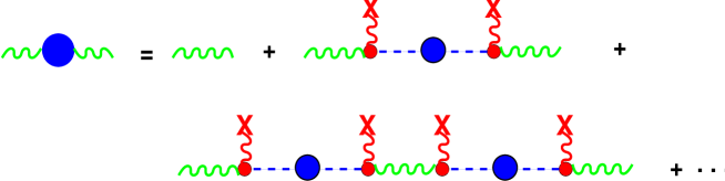
Figure 1: The effective photon propagator obtained by summing up the full series of diagrams with external field insertions (curly lines with a cross) carrying zero momentum. The big bubble in the middle of the dashed lines indicate the exact summation of the scalar/pseudoscalar self-energy.

In our calculation we include also the renormalized self-energy effects in the scalar propagator, summed up to all orders, as indicated in Fig.1 with a bubble inside the scalar propagator (dashed line). Notice that the leading contributions to the scalar self-energy are provided by the one-loop diagrams in which two photons lines are circulating in the loop. As shown later on, these class of diagrams will be crucial for our analysis since they induce a (finite) imaginary part in the scalar self-energy as well as in the effective photon propagator.

Let us choose a gauge where the free photon propagator $D_{ij}(k)$ in momentum space has only spatial components

$$D_{ij}(k)=\frac{i}{k^{2}+i\varepsilon}\delta_{ij}\,,$$ (7)

and zero for all the other ones. From now on, with the symbol $k^{2}$ we indicate $k_{\mu}k^{\mu}$, where $k_{0}=\omega$ and $k_{i}=(\vec{k})_{i}$ are the corresponding energy and 3-momentum, respectively, associated to the photon propagator, and $\delta_{ij}$ is the unit matrix in 3-dimensional space. In this gauge, the result for the effective photon propagator $P^{(S,{\rm B})}_{ij}(k,{\rm\vec{B}})$, induced by the mixing with a scalar field in the presence of an external magnetic field $\vec{\rm B}$, is the following

$$P_{ij}^{(S,{\rm\vec{B}})}(k,{\rm\vec{B}}) = \frac{i}{k^{2}+i\varepsilon}R_{ij}^{(1)}({\rm\vec{B}})+\frac{i}{k^{2}-\Pi^{(1)}(k,{\rm\vec{B}})}T_{ij}^{(1)}({\rm\vec{B}})\,,$$ (8)

where the tensor functions $T_{ij}^{(1)}({\rm\vec{B}})$ and $R_{ij}^{(1)}({\rm\vec{B}})$ are symmetric tensors in the $i,j$ indices, and $T_{ij}^{(1)}({\rm\vec{B}})$ is a projector for $\vec{k}$ and ${\rm\vec{B}}$ vectors, that is satisfying the conditions $k_{i}T_{ij}^{(1)}({\rm\vec{B}})={\rm B}_{i}T_{ij}^{(1)}({\rm\vec{B}})=0$. More explicitly,

$$T_{ij}^{(1)}({\rm\vec{B}}) = \delta_{ij}-\frac{|\vec{\rm B}|^{2}k_{i}k_{j}-\vec{k}\cdot\vec{\rm B}\left(k_{i}{\rm B}_{j}+k_{j}{\rm B}_{i}\right)+|\vec{k}|^{2}{\rm B}_{i}{\rm B}_{j}}{|\vec{k}|^{2}|\vec{\rm B}|^{2}-\left(\vec{k}\cdot\vec{\rm B}\right)^{2}}\,,$$

$$R_{ij}^{(1)}({\rm\vec{B}}) = \frac{|\vec{\rm B}|^{2}k_{i}k_{j}-\vec{k}\cdot\vec{\rm B}\left(k_{i}{\rm B}_{j}+k_{j}{\rm B}_{i}\right)+|\vec{k}|^{2}{\rm B}_{i}{\rm B}_{j}}{|\vec{k}|^{2}|\vec{\rm B}|^{2}-\left(\vec{k}\cdot\vec{\rm B}\right)^{2}}\,,$$ (9)

and the expression for scalar part of photon self-energy $\Pi^{(1)}(k,{\rm\vec{B}})$ induced by the external magnetic field $\vec{\rm B}$ is given by

$$\Pi^{(1)}(k,{\rm\vec{B}})=\frac{1}{|\Lambda_{S}|^{2}}\,\frac{|\vec{k}|^{2}|\vec{\rm B}|^{2}\,\sin^{2}{\theta}}{k^{2}-m_{S}^{2}-\Sigma_{S}(k^{2})}\,,$$ (10)

where $m_{S}$ and $\Sigma_{S}(k^{2})$ are the renormalized mass and self-energy of the exchanged scalar boson, and $\theta$ is the angle between the direction of the photon momentum $\vec{k}$ and the external magnetic field ${\rm\vec{B}}$. Notice that the first term on the right hand side of Eq.(8), which includes the contribution of longitudinal polarizations, depends on the gauge choice in Eq.(7), whereas the second term in Eq.(8) is gauge independent. The latter property comes from the transversality of $T_{ij}^{(1)}({\rm\vec{B}})$ tensor, namely $k_{i}T_{ij}^{(1)}({\rm\vec{B}})=0$.

The physical interpretation of the $T_{ij}^{(1)}({\rm\vec{B}})$ and $R_{ij}^{(1)}({\rm\vec{B}})$ is clear. The $R_{ij}^{(1)}({\rm\vec{B}})$ represents the contribution of both longitudinal and transverse photon polarization components, while $T_{ij}^{(1)}({\rm\vec{B}})$ represents the contribution of the transverse polarization orthogonal to both $\vec{\rm B}$ and $\vec{k}$. This picture is largely simplified by choosing the momentum $\vec{k}$ direction orthogonal to the external field that is $\vec{k}\cdot\vec{\rm B}=0$. Then

$$T_{ij}^{(1)}({\rm\vec{B}})=\delta_{ij}-\frac{k_{i}k_{j}}{|\vec{k}|^{2}}-\frac{{\rm B}_{i}{\rm B}_{j}}{|\vec{\rm B}|^{2}}\,,~{}~{}~{}~{}~{}~{}~{}R_{ij}^{(1)}({\rm\vec{B}})=\frac{k_{i}k_{j}}{|\vec{k}|^{2}}+\frac{{\rm B}_{i}{\rm B}_{j}}{|\vec{\rm B}|^{2}}\,.$$ (11)

As expected from the structure of the interaction vertex, the external magnetic field modifies the photon dispersion relations only for the transverse polarization component which is orthogonal to the plane generated by external magnetic field direction and the photon momentum. This modification is contained in the denominator of the second term of Eq.(8) due to the self-energy correction $\Pi^{(1)}(k,\vec{{\rm B}})$ in Eq.(10).

Now we consider the case of a scalar field coupled to an external electric field ${\rm\vec{E}}$. By retaining only the linear terms in the external field, the relevant interaction Lagrangian is given by

$$L_{\rm int}^{S}({\rm\vec{E}})=-\frac{1}{\Lambda_{S}}\,{\rm\vec{E}}\cdot\left(\frac{\partial}{\partial t}\vec{A}(x)\right)\varphi_{S}(x)\,.$$ (12)

The corresponding Feynman rule is in this case given by

where ${\rm E}_{i}$ is the $i$-th component of the external electric field ${\rm\vec{E}}$ and $\omega$ is the corresponding energy of the photon whose four-momentum is entering the vertex. Notice that the expression of the Lagrangian in Eq.(12) depends on the adopted choice of temporal gauge $A_{0}=0$. However, it is worth stressing that the photon dispersion relations, being an observable physical effect, will not depend on the gauge choice.

In analogy with the external magnetic field, the effective photon propagator induced by an external electric field can be straightforwardly derived by summing up the self-energy diagrams to all orders as above. By using the same gauge condition as in Eq.(7) for the free photon propagator, the result for the effective photon propagator is the following

$$P_{ij}^{(S,{\rm\vec{E}})}(k,{\vec{E}}) = \frac{i}{k^{2}+i\varepsilon}R_{ij}^{(2)}({\rm\vec{E}})+\frac{i}{k^{2}-\Pi^{(2)}(k,{\rm\vec{E}})}T_{ij}^{(2)}({\rm\vec{E}})\,.$$ (13)

where $T_{ij}^{(2)}({\rm\vec{E}})$ and $R_{ij}^{(2)}({\rm\vec{E}})$ are given by

$$T_{ij}^{(2)}{({\rm\vec{E}})}=\frac{{\rm E}_{i}{\rm E}_{j}}{|\vec{\rm E}|^{2}}\,,~{}~{}~{}~{}~{}~{}~{}R_{ij}^{(2)}{({\rm\vec{E}})}=\delta_{ij}-\frac{{\rm E}_{i}{\rm E}_{j}}{|\vec{\rm E}|^{2}}\,.$$ (14)

The tensor functions $T_{ij}^{(2)}{({\rm\vec{E}})}$ and $R_{ij}^{(2)}{({\rm\vec{E}})}$ represent the contributions of the photon polarization parallel and orthogonal to the external electric field ${\rm\vec{E}}$, respectively. The scalar part of the photon self-energy in the second term of Eq.(13) is given by

$$\Pi^{(2)}(k,{\rm\vec{E}})=\frac{1}{|\Lambda_{S}|^{2}}\,\frac{\omega^{2}\,|\vec{\rm E}|^{2}}{k^{2}-m_{S}^{2}-\Sigma_{S}(k^{2})}\,.$$ (15)

In the case of an angle $\theta\neq\pi/2$ formed by the momentum $\vec{k}$ of the incident wave and the direction of the external electric field $\vec{\rm E}$, the formula in Eq.(15) will be modified as

$$\Pi^{(2)}(k,{\rm\vec{E}})=\frac{1}{|\Lambda_{S}|^{2}}\,\frac{\omega^{2}\,|\vec{\rm E}|^{2}\sin^{2}{\theta}}{k^{2}-m_{S}^{2}-\Sigma_{S}(k^{2})}\,.$$ (16)

and the corresponding photon polarization will be the one parallel to the plane formed by the momentum $\vec{k}$ and the external field $\vec{\rm E}$.

Contrary to the case of an external magnetic field, the external electric field modifies the photon dispersion relations only for the photon polarization component which is parallel to the plane formed by $\vec{E}$ and $\vec{k}$, while the orthogonal component remains unaffected. The modification of dispersion relations is contained in the denominator of the second term of Eq.(13) due to the self-energy correction $\Pi^{(2)}(k,{\rm\vec{E}})$ in Eq.(16).

Analogous results for a pseudoscalar field minimally coupled to two photons as in Eq.(2) can be obtained in a straightforward way from the above results. In particular, for a pseudoscalar field the relevant interaction Lagrangian, linear in the external field, these are given by

$$L_{\rm int}^{P}({\rm\vec{E}})=\frac{1}{\Lambda_{P}}\,\vec{\rm E}\cdot\left(\vec{\nabla}_{x}\wedge\vec{A}(x)\right)\varphi_{P}(x)\,,$$ (17)

$$L_{\rm int}^{P}({\rm\vec{B}})=-\frac{1}{\Lambda_{P}}\,{\rm\vec{B}}\cdot\left(\frac{\partial}{\partial t}\vec{A}(x)\right)\varphi_{P}(x)\,.$$ (18)

By comparing the Lagrangians in Eqs.(6), (12) with the corresponding ones in Eqs.(17), (18) it is easy to derive the effective photon propagator by using the previous results for the scalar case. In particular, for the effective photon propagator induced by a pseudoscalar field in the presence of external magnetic or electric field, one obtains

$$P_{ij}^{(P,{\rm{\vec{B}}})}(k,{\rm{\vec{B}}}) = \frac{i}{k^{2}+i\varepsilon}R_{ij}^{(2)}({\rm\vec{B}})+\frac{i}{k^{2}-\Pi^{(2)}(k,{\rm\vec{B}})}T_{ij}^{(2)}({\vec{\rm B}})\,,$$ (19)

$$P_{ij}^{(P,\vec{\rm E})}(k,{\rm{\vec{E}}}) = \frac{i}{k^{2}+i\varepsilon}R_{ij}^{(1)}({\rm\vec{E}})+\frac{i}{k^{2}-\Pi^{(1)}(k,{\rm\vec{E}})}T_{ij}^{(1)}({\rm\vec{E}})\,,$$ (20)

provided that inside the functions $T_{ij}^{(1)}({\rm\vec{E}})$, $R_{ij}^{(1)}({\rm\vec{E}})$, $T_{ij}^{(2)}({\rm\vec{B}})$, $R_{ij}^{(2)}({\rm\vec{B}})$, $\Pi^{(2)}(k,{\rm\vec{B}})$, and $\Pi^{(1)}(k,{\rm\vec{E}})$, appearing in Eqs.(19),(20), the following substitutions $\Lambda_{S}\to\Lambda_{P}$, $m_{S}\to m_{P}$, and $\Sigma_{S}(k^{2})\to\Sigma_{P}(k^{2})$ for the corresponding pseudoscalar quantities are implemented.

3 The photon dispersion

In order to derive the new dispersion relations for the propagating photon induced by the external field, we first look at the zeros connected to the inverse of the real part of photon propagators in the last terms of Eqs.(8), (13) and (19), (20). In particular, this consists in solving the following mass-gap equations

• Scalar

  $${\rm External~{}~{}~{}\vec{B}}~{}~{}~{}~{}\to~{}~{}~{}~{}k^{2}-{\rm Re}\,[\Pi^{(1)}(k,{\rm\vec{B}})] = 0\,,$$

  $${\rm External~{}~{}~{}\vec{E}}~{}~{}~{}~{}\to~{}~{}~{}~{}k^{2}-{\rm Re}\,[\Pi^{(2)}(k,{\rm\vec{E}})] = 0\,,$$ (21)

• Pseudoscalar

  $${\rm External~{}~{}~{}\vec{B}}~{}~{}~{}~{}\to~{}~{}~{}~{}k^{2}-{\rm Re}\,[\Pi^{(2)}(k,{\rm\vec{B}})] = 0\,,$$

  $${\rm External~{}~{}~{}\vec{E}}~{}~{}~{}~{}\to~{}~{}~{}~{}k^{2}-{\rm Re}\,[\Pi^{(1)}(k,{\rm\vec{E}})] = 0\,.$$ (22)

The fact that there is the presence of an external field, does not guarantee anymore that the equations above have a unique solution at $k^{2}=0$, as expected instead in the case of vanishing external sources.

However, we will see that not all the solutions of Eq.(22) will correspond to physical ones, and there will appear a spurious solution. In particular, in order to link the solutions to the physical spectrum, the following conditions must be fulfilled:

• the square of the photon energy $\omega$ must be real and positive, namely $\omega^{2}>0$;

• the residue at the pole of the propagator must be positive, in order to ensure that the corresponding quantum state has a positive norm.

We will show that the above equations admit at most two acceptable solutions which satisfy the above criteria. This can also be seen by switching off the imaginary part of the scalar/pseudoscalar self-energy. In this case the equations above become quadratic in $k^{2}$ and only two solutions are generated, corresponding to the classical ones [16]. One of these solutions corresponds to a light-like mode ($\omega=|\vec{k}|/n$) with a refraction index $n>1$, while the other one can be associated to a massive mode ($\omega^{2}\simeq|\vec{k}|^{2}+M^{2}$) with a mass $M$ very close to the mass of the exchanged scalar or pseudoscalar particle. Indeed, the total number of degrees of freedom must be conserved. In the original Lagrangian there are three degrees of freedom corresponding to particles which are on-shell, the two photon components and the scalar/pseudoscalar field. The number of physical poles are indeed three, the two mentioned above and the pole at $k^{2}=0$ related to the photon polarization which does not interact with the external field.

As we will show later on, the inclusion of the quantum corrections, which are absorbed in the scalar/pseudoscalar self-energy, cannot be neglected due to the presence of an imaginary part in the scalar/pseudoscalar self-energy $\Sigma(k^{2})$ induced by the interaction in Eqs.(1) and (2). Then, the massive dispersion mode would be allowed provided that the external field is above some particular critical value, which depends on the mass and decay width of the exchanged scalar/pseudoscalar particle and photon energy.

Now we will provide the solutions to the mass-gap equations in Eqs.(21), (22). The exact results are given in the appendix A, while below we will report the approximated expressions obtained by expanding the exact solutions in powers of a small parameter contained in the photon self-energy $\Pi^{(1,2)}(\Delta,k)$. In order to simplify the notation, it is convenient to compactify the set of Eqs.(21) and (22) as follows

$$k^{2}-{\rm Re}\,\left[\Pi(k,\Delta)\right]=0$$ (23)

where $\Pi(k,\Delta)$ generically stands for the effective photon self-energy and it is given by

$$\Pi(k,\Delta)=\frac{\Delta}{k^{2}-m^{2}-\Sigma(k^{2})}\,.$$ (24)

Above, $m$ and $\Sigma(k^{2})$ indicate the renormalized mass and self-energy of the exchanged scalar or pseudoscalar particle, respectively. In Eq.(24), the term $\Delta$ absorbs the contribution of the external field interaction and it is given by $\Delta=\Delta^{(1)}({\rm\vec{B}})$ and $\Delta=\Delta^{(2)}({\rm\vec{E}})$ for a scalar field in the presence of an external magnetic and electric fields, where

$$\Delta^{(1)}({\rm\vec{B}})=\frac{|\vec{k}|^{2}|\vec{\rm B}|^{2}\,\sin^{2}{\theta}}{|\Lambda_{S}|^{2}}\,,~{}~{}~{}~{}\Delta^{(2)}({\rm\vec{E}})=\frac{\omega^{2}\,|\vec{\rm E}|^{2}\sin^{2}{\theta}}{|\Lambda_{S}|^{2}}\,$$ (25)

and similarly, $\Delta=\Delta^{(1)}({\rm\vec{E}})$ and $\Delta=\Delta^{(2)}({\rm\vec{B}})$ for the pseudoscalar case.

By separating the real and imaginary part in Eq.(24), the Eq.(23) can be written as

$$k^{2}-\frac{\Delta\left(k^{2}-m^{2}-{\rm Re}[\Sigma(k^{2})]\right)}{\left(k^{2}-m^{2}-{\rm Re}\,[\Sigma(k^{2})]\right)^{2}+\left({\rm Im}\,\left[\Sigma(k^{2})\right]\right)^{2}}=0\,.$$ (26)

When $k^{2}=m^{2}$, the term $m^{2}-{\rm Re}[\Sigma(m^{2})]$ corresponds to the renormalized scalar or pseudoscalar mass, including radiative corrections. However, it is convenient to adopt the so-called on-shell mass renormalization scheme where ${\rm Re}[\Sigma(k^{2})]|_{k^{2}=m^{2}}=0$. Then, from now on, $m^{2}$ will stand for the renormalized mass. On the other hand, ${\rm Im}[\Sigma(k^{2})]$ is finite at 1-loop, being connected to the tree level decay in two massless photons. In particular, see Appendix B for more details, for scalar (pseudoscalar) interaction we have

$${\rm Im}[\Sigma(k^{2})]=-\frac{(k^{2})^{2}}{64\pi\Lambda^{2}_{S(P)}}\,.$$ (27)

We stress here that the threshold where the imaginary part of the scalar/pseudoscalar self-energy ${\rm Im}[\Sigma(k^{2})]$ is different from zero starts at $k^{2}=0$, due to the fact that a scalar/psedusocalar particle with two photon interaction can always decay in two massless photons, regardless of the size of its mass. We will see that the effects of the external field corrections, will shift this threshold above $k^{2}>0$ due to the modification of the photon refraction index, see section 4.2 for more details.

In the physical scenarios that we are considering here, there is a characteristic (small) dimensionless parameter which is given by $\Delta/m^{4}$. Its smallness is due to the fact that the $\Delta\sim 1/\Lambda_{S,P}^{2}$ where the effective scale $\Lambda_{S,P}$ is much larger than any other characteristic energy scale present in our problem, namely $\Lambda^{2}_{S,P}\gg\left\{|{\rm\vec{B}}|,|{\rm\vec{E}}|,\omega^{2},m^{2}\right\}$. This observation will simplify the analysis regarding the solutions of Eq.(26). An approximate solution can indeed be easily found by using the Taylor expansion in terms of $\Delta/m^{4}$. By looking at Eq.(26) one can see that there is always a solution around the massless pole $k^{2}\simeq 0$, which can be parametrized as $k^{2}=\varepsilon_{0}$, with $\varepsilon_{0}/m^{2}$ of order $\Delta/m^{4}$. This corresponds to the dispersion mode where the effects of external field modifies the refraction index of the vacuum, as for instance in the case of QED vacuum polarization in the presence of an external magnetic field [21]. However, as discussed before, Eq.(26) admits also a massive solution provided that $\Delta/({\rm Im}[\Sigma(m^{2})])^{2}\gg 1$. As we will show later on, this inequality will imply the existence of a critical value for the external field.

The Eq.(26), being a cubic equation in $k^{2}$, admits three solutions, namely $k^{2}=M^{2}_{0},~{}M^{2}_{\pm}$. The general expressions are given in the appendix A. However, approximated solutions can be easily found by using the following antsatz

$$k^{2} = \varepsilon_{0}$$ (28)

$$k^{2} = m^{2}+\varepsilon_{m}\,,$$ (29)

By substituting these expressions in Eq.(26) and neglecting higher order terms ${\cal O}(\varepsilon_{0}^{2}/m^{4})$ and ${\cal O}(\varepsilon_{m}^{2}/m^{4})$, the algebraic equations in $k^{2}$ can be split into a linear and quadratic ones for $\varepsilon_{0}$ and $\varepsilon_{m}$, respectively. We get the following results

$$M^{2}_{0} = -\frac{\Delta}{m^{2}}\,,$$

$$M^{2}_{\pm} = m^{2}+\frac{\Delta}{2m^{2}}\left(1\pm\sqrt{1-\xi}\right)\,,$$ (30)

where

$$\xi~{}\equiv~{}\frac{4m^{6}\Gamma^{2}}{\Delta^{2}}\,,$$ (31)

and $\Gamma$ is the scalar (or pseudoscalar) width given by ${\rm Im}[\Sigma(m^{2})]=-m\Gamma$. As shown in the appendix A, these results can also be easily obtained from the exact expressions by retaining the leading order terms in the $\Delta/m^{4}$ expansion. In the value of $\Gamma$ we absorb all the effects of the external fields corrections on the scalar/pseudoscalar decay width. However, it is reasonable to assume that these corrections are sub-leading for our problem and for practical purposes we neglect them and retain only the tree-level contributions to the scalar/pseudoscalar width induced by the interactions in Eqs.(1),(2). In order to have real solutions for $m^{2}$, the condition $\xi>1$ must be satisfied. We will return on this point after discussing the dispersion relations.

As previously discussed, the lightest mode ($M_{0}$) corresponds to the propagation of a photon in a medium with a refraction index $n$ given by

$$n^{(S)}({\rm\vec{B}}) \simeq 1+\frac{|\vec{\rm B}|^{2}\,\sin^{2}{\theta}}{2m^{2}|\Lambda_{S}|^{2}}$$ (32)

$$n^{(S)}({\rm\vec{E}}) \simeq 1+\frac{|\vec{\rm E}|^{2}\,\sin^{2}{\theta}}{2m^{2}|\Lambda_{S}|^{2}}\,.$$ (33)

where $n$ is usually defined as $n\equiv|\vec{k}|/\omega$. Above, $n^{(S)}({\rm\vec{B}})$ ($n^{(S)}({\rm\vec{E}})$) stands for the refraction index in magnetic (electric) external fields with scalar interactions. Analogous results are obtained for the pseudoscalar case, with $n^{(P)}({\rm\vec{B}})=n^{(S)}({\rm\vec{E}})$ and $n^{(P)}({\rm\vec{E}})=n^{(S)}({\rm\vec{B}})$  , where the substitution of $\Lambda_{S}\to\Lambda_{P}$ in $n^{(S)}({\rm\vec{B}})$ and $n^{(S)}({\rm\vec{E}})$ is understood. The next leading order corrections in $\Delta/m^{4}$ to the dispersion relations gives the non linear dependence of the refraction index with the photon energy. From now on in our notation, whenever the energy ($\omega$) dependence in the refraction index $n(\omega)$ is not explicitly shown, it means that it corresponds to $n(\omega=0)$.

Regarding the other massive solutions $k^{2}=M^{2}_{\pm}$ of Eq.(26), only one is physically acceptable and it will correspond to the pole $k^{2}=M^{2}_{+}$. This can be easily seen by taking the limit $\Gamma\to 0$ or analogously $\xi\to 0$, where one should recover the classical $(\Gamma=0)$ solution $k^{2}=m^{2}+\frac{\Delta}{m^{2}}$ [16]. This massive pole should correspond to the propagation of a particle of mass $m=M_{+}$ provided that the square of the mass term $M^{2}_{+}$ is a real and positive quantity. At this point it is convenient to define the following dimensionless parameters $x_{E,B}$ by $x_{B}=\frac{|\vec{\rm B}|^{2}\sin^{2}{\theta}}{2m^{2}\Lambda_{S}^{2}}$ and $x_{E}=\frac{|\vec{\rm E}|^{2}\sin^{2}{\theta}}{2m^{2}\Lambda_{S}^{2}}$. In our problem $x_{E,B}\ll 1$ and one can simplify the dispersion relations above by expanding them around $x_{E,B}=0$. In particular, for the scalar case, by using the approximate solutions in Eq.(30), we have for the massive mode in the presence of external electric and magnetic fields

• External    ${\bf\vec{B}}$

  $$\omega^{2}\simeq|\vec{k}|^{2}\left\{1+x_{B}\left(1+\sqrt{1-\frac{4\Gamma^{2}m^{6}\Lambda^{4}}{|{\rm\vec{B}}|^{4}\sin^{4}{\theta}|\vec{k}|^{4}}}\right)\right\}+m^{2}\,,$$ (34)

• External    ${\bf\vec{E}}$

  $$\omega^{2}\simeq\left(|\vec{k}|^{2}+m^{2}\right)\left\{1+x_{E}\left(1+\sqrt{1-\frac{\Gamma^{2}m^{2}}{x_{E}^{2}\left(|\vec{k}|^{2}+m^{2}\right)^{2}}}\right)\right\}\,,$$ (35)

where terms of order ${\cal O}(x_{B,E}^{2})$ have been neglected. Analogous results for the pseudoscalar case are obtained by using for the external magnetic and electric fields the expressions in Eq.(35) and Eq.(34), respectively, and by substituting $\Lambda_{S}\to\Lambda_{P}$.

One can easily see that, in order to have a real solution for $\omega^{2}$, see Eq.(30), the following condition must be satisfied

$$\Delta~{}\geq~{}2\,m^{3}\,\Gamma\,.$$ (36)

Notice that in the classical approximation [16], no condition is required for all the parameters in the Lagrangian in order to have a massive pole in the spectrum. Indeed, if one sets $\Gamma\to 0$, the condition (36) is always satisfied. However, we emphasize that the approximation of neglecting the width $\Gamma$ in the axion physics, as usually done in all previous studies, is well justified due to the very small axion mass. Indeed, for characteristic magnetic fields of the order of Tesla, axion masses of the order of meV, and photons wave lengths in the optical region, the condition (36) is always satisfied, provided that the contribution to the total width is dominated by the axion decay in two photons.

The physical meaning of Eq.(36) can be roughly understood as follows. Let us consider the case in which the width $\Gamma$ is very large in comparison with the mass scale set by the quantity $\Delta$, in such a way that the relation (36) cannot be satisfied. In this case, the fact that the scalar/pseudoscalar particle can decay too fast does not allow the massive photon mode to be formed and hence cannot coherently propagate.

Given a particular value for the photon energy $\omega$, the inequality above leaves to the following critical values for the magnetic and electric external fields for a scalar interaction

$$|{\rm\vec{B}}| \geq {\rm B}_{\rm crit}\equiv\frac{m^{\frac{3}{2}}\,\sqrt{2\Gamma}\,|\Lambda_{S}|}{|\vec{k}\sin{\theta}|}\sqrt{1+R(\delta)}$$

$$|{\rm\vec{E}}| \geq {\rm E}_{\rm crit}\equiv\frac{m^{\frac{3}{2}}\,\sqrt{2\Gamma}\,|\Lambda_{S}|}{\omega|\sin{\theta}|}\sqrt{1+R(\delta)}$$ (37)

and analogously for pseudoscalar one

$$|{\rm\vec{E}}| \geq {\rm E}_{\rm crit}\equiv\frac{m^{\frac{3}{2}}\,\sqrt{2\Gamma}\,|\Lambda_{P}|}{|\vec{k}\sin{\theta}|}\sqrt{1+R(\delta)}$$

$$|{\rm\vec{B}}| \geq {\rm B}_{\rm crit}\equiv\frac{m^{\frac{3}{2}}\,\sqrt{2\Gamma}\,|\Lambda_{P}|}{\omega|\sin{\theta}|}\sqrt{1+R(\delta)}\,.$$ (38)

where $|\vec{k}|\simeq\sqrt{\omega^{2}-m^{2}}\,+\,{\cal O}(x_{B,E})$. The expression for the function $R(x)\sim{\cal O}(x)$, containing the higher-order corrections in powers of $\delta=\Gamma/m$, is reported in the appendix A. Analogously, for a fixed value of the external field, the conditions above can be read as the minimum photon energy $\omega$ necessary in order to generate a massive mode. We have explicitly checked that the approximated solutions in Eq.(30) are obtained from the exact ones by retaining only the leading contribution in the weak external field expansion. See Appendix A for more details.

A remarkable aspect of the results in Eqs.(37), (38) is that in the case in which the scalar or pseudoscalar field has only the decay mode in two photons, the critical value for the external field does not depend on the coupling $\Lambda$ of the effective interaction. This can be easily checked by noticing that the corresponding width $\Gamma$ in that case would be proportional to $\Gamma\propto m^{3}/\Lambda^{2}$, while $\Delta\propto 1/\Lambda^{2}$.

In order to identify the massive poles in the effective propagator as physical quantum states, one has to check that the corresponding residue at the pole of the propagator is positive. Indeed, the residue at the pole ($Z$) is connected by unitarity to the norm of the quantum state excited from the vacuum. In particular, for a generic solution $k^{2}=M^{2}$ of the mass gap equation, one gets

$$Z\equiv\lim_{k^{2}\to{\rm M}^{2}}\left(k^{2}-{\rm M}^{2}\right)\left(k^{2}-{\rm Re}\,\Pi(k,\Delta)\right)^{-1}\,.$$ (39)

or equivalently

$$Z=\left(1-\frac{\partial}{\partial k^{2}}{\rm Re}\,\Pi(k,\Delta)\Big{|}_{k^{2}={\rm M}^{2}}\right)^{-1}\,.$$ (40)

where $Z^{1/2}$ is the wave function renormalization constant.

By using the expression in Eq.(40), we find the following result for the residue at the poles $k^{2}=M_{0}^{2}$ and $k^{2}=M_{\pm}^{2}$, respectively $Z_{0}$ and $Z_{\pm}$

$$Z_{0} = 1-\frac{\Delta}{m^{4}}\,,$$ (41)

$$Z_{\pm} = \pm\,\frac{\Delta}{2m^{4}}\frac{\left(1\pm\sqrt{1-\xi}\right)}{\sqrt{1-\xi}}\,,$$ (42)

where we have neglected terms of the order ${\cal O}(\frac{\Delta^{2}}{m^{8}})$. As we can see from these results, two physical solutions are allowed, corresponding to the positive norm states of $Z_{0}>0$ and $Z_{+}>0$, connected respectively to the poles $k^{2}=M^{2}_{0}$ and $k^{2}=M^{2}_{+}$, while $k^{2}=M^{2}_{-}$ is an unphysical one, being associated to a ghost ($Z_{-}<0$).

Notice that when the external field is far above the critical value, $\xi\ll 1$, but still in the weak coupling regime i.e. $\Delta/m^{4}\ll 1$, then the term $Z_{+}\simeq{\cal O}(\Delta/m^{4})\ll 1$. This means that in this case the probability to induce the massive mode from the vacuum, is very suppressed. However, when we approach the critical value $\xi\to 1$ the constant $Z_{+}$ increases and tends to infinity at $\xi=1$.

This behavior can be easily understood if we look at the inverse of the propagator $\Pi^{-1}(k^{2})$ near the pole $k^{2}\simeq M^{2}$, in particular

$$\Pi^{-1}(k^{2})|_{k^{2}\simeq M^{2}}=(k^{2}-M^{2})Z^{-1}+(k^{2}-M^{2})^{2}\,{\rm Re}\Sigma^{{}^{\prime\prime}}(M^{2})|_{k^{2}=M^{2}}+\dots\,+i\,{\rm Im}\Sigma(M^{2})$$ (43)

where the dots stand for higher order terms in $(k^{2}-M^{2})/m^{2}$ expansion, and $\Sigma^{{}^{\prime\prime}}(M^{2})$ indicates the second derivative of $\Sigma(k^{2})$ with respect to $k^{2}$ and evaluated at $k^{2}=M^{2}$. Notice that $\xi=1$ corresponds to two degenerate massive solutions, and the propagator generates a double pole in $k^{2}=M^{2}_{+}=M^{2}_{-}$. This is not a matter of the approximation adopted, since the same conclusions are obtained in the exact case (see Appendix A for more details). Clearly, since $Z^{-1}$ is related to the coefficient of the single pole, $Z^{-1}$ vanishes at $\xi\to 1$ or analogously $Z\to\infty$. Moreover, since the $Z$ factor is related by unitarity to the probability of creating the corresponding quantum state from the vacuum, when $Z>1$ the unitarity is spoiled. Therefore, the requirement of unitarity sets a region of validity of our calculations when the external field is close to its critical value. By imposing $Z_{+}\leq 1$ we obtain

$$0\leq\xi\leq 1-\frac{\Gamma^{2}}{m^{2}}+{\cal O}(\frac{\Gamma^{3}}{m^{3}})\,.$$ (44)

In conclusion, the probability that the massive mode is excited from the vacuum increases as the external field approaches (from above) the critical value, but clearly vanishes just below the critical value.

4 The photon absorption coefficient

Due to the presence of an external constant electric or magnetic field, the interactions in Eqs.(1), (2) can induce a non-vanishing probability for the photon splitting amplitude $\gamma\to\gamma\gamma$. This phenomenon is well known in the framework of QED [21], as well as the analogous one of electron-pair creation $\gamma\to e^{+}e^{-}$ in constant and homogeneous magnetic field [22, 23]. Nevertheless, there are no studies so far concerning the analogous effect of photon conversion process $\gamma\to\gamma\gamma$ induced by the scalar and pseudoscalar interactions. Measurement of a photon splitting in constant magnetic field is a challenge for experiment, although high-energy photon splitting in atomic fields has been recently observed [25].

For this kind of problem it is appropriate to express the conversion probability in terms of a photon attenuation coefficient, usually called absorption coefficient ($d_{\gamma}$) [23]. In particular, the number $N_{\gamma\gamma}$ of photon splitting events created by a photon crossing an EM background field for a path length $L$ are given by

$$N_{\gamma\gamma}=N_{\gamma}\left(1-\exp\left[-d_{\gamma}\,L\right]\right)\simeq\,N_{\gamma}d_{\gamma}\,L$$ (45)

where $N_{\gamma}$ is the total number of photons entering the background EM field. Notice that the last relation is a good approximation only when $d_{\gamma}L\ll 1$.

Due to the photon interactions in Eqs.(1), (2), a new kind of contribution to the photon absorption coefficient $d_{\gamma}$ is expected with respect to the corresponding vacuum polarization effects in QED [21, 22, 23]. Now, before entering into the analysis of the new physics contributions, let us start by recalling the known results on the photon propagating in a constant magnetic field [21].

In QED, the matrix element for the $\gamma\to\gamma\gamma$ process can be calculated in perturbation theory by using the Euler-Heisenberg effective Lagrangian [26] arising from integrating out electrons at 1-loop. After expanding the electromagnetic field around the constant background field, new dispersions relations are obtained for the photon propagating in the external field. A refraction index $(n_{(\lambda)}>1)$ associated to the photon polarization $\varepsilon_{\mu}(\lambda)$, where $\lambda$ parametrizes the two polarizations parallel and perpendicular to the magnetic field direction, arises. Even by neglecting the dispersion effects, the photon splitting process $\gamma\to\gamma\gamma$ is kinematically allowed, provided that all particle momenta in the reaction are proportional to a unique momentum $k_{\mu}$, satisfying $k^{2}=0$. However, as shown in Ref.[21], at least three external field insertions would be necessary in order to have a non-vanishing matrix element. This is a simple consequence of the Lorentz and gauge invariant structure of the Euler-Heisenberg Lagrangian and due to the fact that there is only one light-like four-momentum in the process. The magnitude of the resulting photon splitting absorption coefficient would then given by [21]:

$$d_{\gamma}^{\rm QED}\simeq\,0.1\left(\frac{{\rm B}}{{\rm B}_{\rm cr}^{\rm QED}}\right)^{6}\left(\frac{\omega}{m_{e}}\right)^{5}\,{\rm cm}^{-1}\,,$$ (46)

where ${\rm B}_{\rm cr}^{\rm QED}=\frac{m_{e}^{2}}{e}$, with $e$ the unity of electric charge, is the critical magnetic field for the photon-pair creation [22, 23] and $m_{e}$ is the electron mass. This formula holds only for $\theta=\pi/2$ and in the weak-field limit $e{\rm B}/m_{e}^{2}\ll 1$. Then, one can see that even for strong laboratory magnetic fields (of the order of Tesla) the absorption coefficient $d_{\gamma}$ would be very small, due to the fact that $B_{\rm cr}^{\rm QED}\sim 10^{10}$ Tesla. Only in astrophysical context this effect can become relevant. In particular, with pulsar magnetic fields of the order of $B_{\rm cr}^{\rm QED}$ and $\omega\simeq m_{e}$, there are many photon splitting absorption lengths in a characteristic pulsar distance of $10^{6}$cm. By taking into account the dispersive effects, the energy-momentum conservation is modified. The momenta of the two final photons will not be parallel anymore and differ from each other for small angles. Due to the dispersive effects, the matrix element of the photon splitting can be induced by one external field insertion. However, in this case the corresponding $d_{\gamma}$ would turn out very suppressed by kinematical factors being proportional to the small opening angle of the final photons. [21].

Returning to our case, a practical way to calculate the absorption coefficient from the photon self-energy in Eq.(24) is by making use of the optical theorem which connects $d_{\gamma}$ to the imaginary part of the self-energy evaluated at the corresponding poles of the propagator. As can be seen from Eq.(10), the imaginary part of photon self-energy ${\rm Im}\Pi(k,\Delta)$ is then proportional to the imaginary part of the scalar/pseudoscalar self-energy, namely ${\rm Im}\,\Pi(k,\Delta)\propto{\rm Im}\Sigma(k^{2})$.

Now, if we do not take into account the effects of vacuum polarization in background EM field, and consider the photon purely massless, the kinematics of the reaction $\gamma\to\gamma\gamma$ would not forbid this process provided that all the momenta are proportional to a unique light-like momentum $k^{2}=0$. However, as in the analogous case of QED, due to the fact that there is only one independent light-like four momentum and due to the antisymmetric property of the electromagnetic field strength $F_{\mu\nu}$, the minimum number of external field insertions is equal to three in order to have a non vanishing effect in the matrix element. This is a general result, as proved by Adler [21], and does not depend on the structure of the interaction, but on the gauge and Lorentz invariant property of the effective Lagrangian for the photon obtained after integrating out the other degrees of freedom. In the case of weak magnetic fields, this would lead into a very strong suppression. As we will show later on, if dispersion effects are taken into account, ($k^{2}=M_{0}^{2}$), the process could proceed by means of one external field insertion only, but suppressed by the small angle induced by the dispersions effects. In the next two sub-sections we will analyze the photon splitting phenomenon induced by the massive and massless dispersion modes respectively.

4.1 Massive dispersion mode

As shown in the previous section, the massive mode of the photon, with mass of the order of the scalar/pseudoscalar one ($m$), is allowed by dispersion relations when the critical conditions in Eqs.(37), (38) are satisfied. Then, the massive mode could easily decay in two lighter photons, or in any other kinematically allowed final states $f$ coupled to the intermediate scalar/pseudoscalar particles. In this case, the corresponding width will be proportional to the imaginary part of self-energy evaluated on the massive pole of the photon propagator ($k^{2}=M^{2}_{+}$). In conclusion, the photon could get a non-vanishing decay width ($\Gamma_{\gamma}$), provided that the critical conditions in Eqs.(37), (38) are satisfied and $\omega\raise 1.29167pt\hbox{$\;>$\kern-7.5pt\raise-4.73611pt\hbox{$\sim\;$}}m_{\gamma}$, where $m_{\gamma}\equiv\sqrt{M^{2}_{+}}$.

One can formally define a width ($\Gamma_{\gamma}$) associated to the massive mode by making use of the optical theorem. In particular,

$$m_{\gamma}\,\Gamma_{\gamma}=-Z_{+}\,{\rm Im}\left[\Pi(k,\Delta)\right]\Big{|}_{k^{2}=m^{2}_{\gamma}}\theta(\omega-m_{\gamma})\theta({\rm B}-{\rm B}_{\rm crit})\,,$$ (47)

where $\theta(x)$ is the standard $\theta$-function defined as $\theta(x)=1$ for $x\geq 0$ and $\theta(x)=0$ for $x<0$, and $m_{\gamma}=\sqrt{m^{2}+\frac{\Delta}{2m^{2}}(1+\sqrt{1-\xi})}$. The constant $Z_{+}$ appearing in Eq.(47) is the corresponding residue at the pole, given in Eq.(40). As shown later, the same result for $\Gamma_{\gamma}$ in Eq.(47) can be re-obtained by starting from the matrix element of the transition $\gamma^{*}\to\gamma\gamma$, where $\gamma^{*}$ represents the massive mode of the photon. For the imaginary part of photon self-energy evaluated at the massive pole $k^{2}=m_{\gamma}^{2}$ we have

$${\rm Im}\left[\Pi(k,\Delta)\right]|_{k^{2}=m_{\gamma}^{2}}=-m^{2}\frac{\left(1-\sqrt{1-\xi}\right)}{\sqrt{\xi}}\,.$$ (48)

Then, the $\Gamma_{\gamma}$ is given by

$$\Gamma_{\gamma}=\frac{\Gamma}{\sqrt{1-\xi}}\left(1-\frac{\Gamma}{2m}\frac{\left(1+\sqrt{1-\xi}\right)}{\sqrt{\xi}}\right)\,,$$ (49)

where the last term in parenthesis comes from the first order expansion in $\Delta/m^{4}$ of the $m_{\gamma}$ when expressed in terms of the axion mass $m$. The absorption coefficient $d_{\gamma}$ entering in Eq.(45), is related to the $\Gamma_{\gamma}$ in Eq.(47) by

$$d_{\gamma}=\frac{m_{\gamma}}{\omega}\,\Gamma_{\gamma}\,.$$ (50)

Finally, by inserting the results of Eqs. (42), (47), and (48) into Eq. (50), we obtain

$$d_{\gamma} = \frac{\Gamma}{\sqrt{1-\xi}}\frac{m}{\omega}\,$$ (51)

where we neglected terms of the order ${\cal O}(\Gamma^{2}/m^{2})$. We stress that to be more precise the scalar/pseudoscalar width $\Gamma$ appearing in all the calculations above should be the one evaluated on the massive pole $m_{\gamma}$, that is $\Gamma(m_{\gamma})$, which differs from the width $\Gamma$ evaluated on the scalar/pseudoscalar mass-shell mass $m$ by small terms of order ${\cal O}(\Gamma/m)$. The same argument applies for the mass $m$ appearing in the expression $m\Gamma$ which should be $m_{\gamma}$ rather than $m$.

As explained at the end of the previous section, the restriction on the upper limit $\xi^{\rm max}=1-\frac{\Gamma^{2}}{m^{2}}$ comes from the requirement of unitarity $Z_{+}\leq 1$. Indeed, the validity of the results in Eq.(51) is based on the optical theorem, which holds only under the hypothesis of unitarity. Notice that, for the imaginary part of photon self-energy evaluated on the other pole $k^{2}=M_{-}^{2}$, the corresponding absorption coefficient would have been negative due to the fact that $Z_{-}<0$, pointing out the presence of an unphysical solution.

These results can be easily re-obtained by starting from the standard formula for the absorption coefficient [21] of photon splitting $\gamma(\omega)\to\gamma(\omega_{1})\gamma(\omega_{2})$

$${\rm d}d_{\gamma}=\frac{1}{2\omega}\frac{1}{2}\frac{d^{3}k_{1}}{(2\pi)^{3}2\omega_{1}}\frac{d^{3}k_{2}}{(2\pi)^{3}2\omega_{2}}(2\pi)^{4}\delta^{4}(k-k_{1}-k_{2})\,|M(\gamma\to\gamma\gamma)|^{2}$$ (52)

where $|M(\gamma\to\gamma\gamma)|^{2}$ is the square modulus summed over final state polarization of the corresponding amplitude. The extra factor $1/2$ in front, takes into account for the identical final states of two photons. The amplitude at the leading order can be easily obtained by evaluating the following Feynman diagram

(53)

where the dark and light curly lines represent the massive and massless photon propagation modes of the photon, and the bubble stands for the photon-scalar/pseudoscalar vertex induced by the external field, and the dashed line represents the scalar/pseudoscalar propagator. By taking into account the renormalization of the wave function $Z_{+}$ in the massive mode, as given by Eq.(42), one obtains

$$|M(\gamma\to\gamma\gamma)|^{2}=\frac{Z_{+}\Delta}{(k^{2}-m^{2})^{2}+\Gamma^{2}m^{2}}\sum_{\rm pol}|V_{\gamma\gamma}(k_{1},k_{2})|^{2}$$ (54)

where $V_{\gamma\gamma}(k_{1},k_{2})$ stands for the vertex of scalar/pseudoscalar in two photons and the sum is performed over the final photon polarizations. In particular, for the scalar (pseudoscalar) interactions, $V_{\gamma\gamma}(k_{1},k_{2})=V^{S(P)}_{\gamma\gamma}(k_{1},k_{2})$, with

$$V^{S}_{\gamma\gamma}(k_{1},k_{2}) = \frac{1}{2\Lambda_{S}}\left[(k_{1}\cdot k_{2})g^{\mu\nu}-k_{1}^{\mu}k_{2}^{\nu}\right]\varepsilon_{1\nu}(k_{1})\varepsilon_{2\mu}(k_{2})\,,$$

$$V^{P}_{\gamma\gamma}(k_{1},k_{2}) = \frac{1}{\Lambda_{P}}\left(k_{1}^{\mu}\,\varepsilon_{1}^{\nu}\,k_{2}^{\alpha}\,\varepsilon_{2}^{\beta}\right)\epsilon_{\mu\nu\alpha\beta}\,,$$ (55)

where $\varepsilon_{1}^{\mu}(k_{1})$ and $\varepsilon_{2}^{\mu}(k_{3})$ are the polarization vectors of the two final photons, and $k_{1,2}$ the corresponding four momenta. Then, by evaluating $k^{2}$ on the massive pole $k^{2}=m_{\gamma}^{2}$, Eq.(52) can be re-written as

$${\rm d}d_{\gamma}=\frac{Z_{+}\Delta}{(m_{\gamma}^{2}-m^{2})^{2}+\Gamma^{2}m^{2}}\left\{d\Phi(2\pi)^{4}\delta^{4}(k-k_{1}-k_{2})\,\sum_{\rm pol}|V_{\gamma\gamma}(k_{1},k_{2})|^{2}\right\}\,,$$ (56)

where $d\Phi\equiv\frac{1}{2\omega}\frac{1}{2}\frac{d^{3}k_{1}}{(2\pi)^{3}2\omega_{1}}\frac{d^{3}k_{2}}{(2\pi)^{3}2\omega_{2}}$. Notice that the integral over the phase space in the last term in parenthesis gives just the scalar/pseudoscalar width $\frac{m_{\gamma}}{\omega}\Gamma(m_{\gamma})\simeq\frac{m}{\omega}\Gamma$. Finally, by integrating Eq.(56) and using the identity

$$\frac{Z_{+}\Delta}{(m_{\gamma}^{2}-m^{2})^{2}+\Gamma^{2}m^{2}}=\frac{1}{\sqrt{1-\xi}}\,,$$ (57)

one can easily recover Eq.(51). It is worth noticing that the denominator of the right-hand-side (r.h.s.) of Eq.(56), which is connected to the scalar(pseudoscalar) propagator, is going in resonance since $m_{\gamma}$ is very close to $m$. This effect partially removes the suppression given by the $Z_{+}$ in the numerator, that is the probability to induce the massive mode.

At this point it is fair to say that the results obtained for the absorption coefficient are based on the assumption that the EM background field is constant and homogeneous in all space. This is an approximation since for any practical experiment the external magnetic or electric field has finite extension. However, it is reasonable to believe that the effects of the boundary conditions can be neglected (as in our case) when the extension length $L$ of the external EM background field where the photon is traveling satisfies the condition $L\gg\lambda_{{\gamma}}$, where $\lambda_{{\gamma}}\sim 1/m_{\gamma}$ is the de Broglie wave length associated to the massive mode $k^{2}=m_{\gamma}^{2}$.

Now we analyze two particular limiting cases, the region of external fields very close to the critical value $\xi\simeq 1$, and the large external fields $\xi\ll 1$. It is easy to see that the maximum value of the width, compatible with unitarity, is obtained, as expected, near the resonant region $\xi\to 1$ where the $Z_{+}\to\infty$. By restricting ourself to the region of maximum value of $Z_{+}$ allowed by unitarity, that is $Z_{+}\simeq 1$ and corresponding to $\xi\simeq 1-\Gamma^{2}/m^{2}$, the maximum value of the absorption coefficient is

$$d_{\gamma}^{\rm max}=\frac{m^{2}}{\omega}+{\cal O}(\frac{\Gamma}{m})\,.$$ (58)

In the opposite limit, of very large external fields $\xi\to 0$, the absorption coefficient gets its minimum value given by

$$d^{\rm min}_{\gamma}\,\simeq\,\frac{m\Gamma}{\omega}\,$$ (59)

which is independent of the external field.

In Fig. 2 we plot the function $d_{\gamma}$ normalized to its maximum value $d_{\gamma}^{\rm max}$, versus $\xi$, for some representative values of ratios $\Gamma/m$.

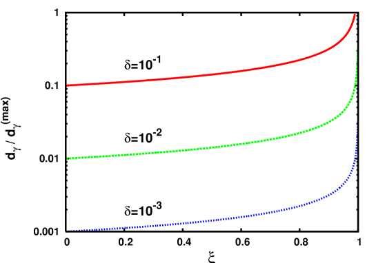
Figure 2: The ratio $d_{\gamma}/d_{\gamma}^{\rm max}$, versus $\xi$, for three values of $\delta=\Gamma/m$, with $\delta=10^{-1},10^{-2},10^{-3}$.

As can be seen from these results, the variation of the photon absorption coefficient as a function of $\xi$ (or analogously as a function of the external field if all the other parameters are taken constants) is very steep only near the region close to the maximum value $\xi^{\rm max}=1-\Gamma^{2}/m^{2}$, when $\Gamma/m\ll 1$. Therefore, for very small values of $\Gamma/m$ the average of $d_{\gamma}$ over the external field could provide a good estimation of the size of the effect, in particular

$$\bar{d}_{\gamma}\,\simeq\,\int_{0}^{1-\frac{\Gamma^{2}}{m^{2}}}d\xi~{}d_{\gamma}=\,\frac{2\Gamma\,m}{\omega}\left(1-\frac{\Gamma}{m}\right)+{\cal O}(\frac{\Gamma^{2}}{m^{2}})\,.$$ (60)

However, notice that the average over the full available range of $\xi$, ($0\leq\xi\leq 1$), is finite and given by $\bar{d}_{\gamma}=\,\frac{2\Gamma\,m}{\omega}(1+{\cal O}(\frac{\Gamma^{2}}{m^{2}}))$. The difference between this result and the one obtained in Eq.(60), with the restricted integration region is a quantity of order ${\cal O}(\Gamma/m)$. This difference should roughly give an idea of the theoretical uncertainty on the absorption coefficient when the average over the external field is considered.

4.2 Massless dispersion mode

Here we consider the possibility that the photon splitting in two photons is induced by the massless dispersion mode $k^{2}=M_{0}^{2}$, see Eqs.(30) and (96). The transition amplitude is given by the Feynman diagram as in Eq.(53), where now the initial photon dispersion corresponds to the massless mode. The evaluation of the absorption coefficient can be easily performed by using the standard formula in Eq.(52), as in the case of QED [21], provided that dispersion relations for the final photons are taken into account. At this point we should stress that if dispersion effects are neglected in the initial and/or final photons propagation modes (that is $n=1$), then the corresponding absorption coefficient vanishes due to the Lorentz covariant structure of the vertex $V_{\gamma\gamma}(k_{1},k_{2})$ in Eq.(55). Indeed, although the process of photon splitting with no-dispersion is not forbidden by kinematics provided that all momenta in the reaction are proportional to a unique momentum satisfying $k^{2}=0$, the square amplitude $\sum_{\rm pol}|V_{\gamma\gamma}(k_{1},k_{2})|^{2}\propto(k_{1}\cdot k_{2})^{2}$ vanishes when $k_{1}^{2}=k_{2}^{2}=k^{2}=0$.

The standard formula for the absorption coefficient remains the same as in Eq.(52) if the dispersion effects are implemented in the delta function as [21]

$$\delta^{4}(k-k_{1}-k_{2})\to\delta(\omega-\omega_{1}-\omega_{2})\delta^{3}(n(\omega)\,\omega\hat{k}-n_{1}(\omega_{1})\,\omega_{1}\hat{k}_{1}-n_{2}(\omega_{2})\,\omega\hat{k}_{2})\,,$$ (61)

where $\omega,\omega_{1,2}$ and $k,k_{1,2}$ are the energy and modulus of the momenta of the corresponding waves respectively, $\hat{k}=\vec{k}/|\vec{k}|$ is the unity vector associated to the momentum $\vec{k}$, and generically $n(\omega)$ is the refraction index where the explicit dependence on the wave energy $\omega$ is shown. According to Ref. [21], the condition set by kinematics in order the reaction to proceed is

$$\Sigma \equiv \omega_{1}n_{1}(\omega_{1})+\omega_{2}n_{2}(\omega_{2})-(\omega_{1}+\omega_{2})n(\omega_{1}+\omega_{2})\,>\,0\,.$$ (62)

This condition can be easily understood by looking at the opening angle $\theta_{12}$ between the two 3-momenta $\vec{k_{1}}$ and $\vec{k_{2}}$ of the final photons, where [21]

$$\theta_{12}=\frac{\omega}{\left(\omega_{1}\omega_{2}\right)^{1/2}}\left(\frac{2\Sigma}{\omega}\right)^{1/2}\,.$$ (63)

In order to have real values for $\theta_{12}$, the condition $\Sigma\geq 0$ must be satisfied.

Let us start by analyzing the case of a photon crossing a constant and homogeneous magnetic field in the presence of a scalar interaction. In order to simplify the analysis we consider the case of a linearly polarized wave with momentum $\vec{k}$ perpendicular to the magnetic field direction. As a first approximation, we neglect the effects of the external field on the QED vacuum polarization. As we will show later on, this approximation can be well justified for typical mass and coupling $\Lambda$ in the range of $m\sim 10^{-3}$eV and $\Lambda\sim 10^{6}$GeV, as suggested for instance by the results of PVLAS experiment [17], or in general for $\sqrt{m\Lambda}\raise 1.29167pt\hbox{$\;<$\kern-7.5pt\raise-4.73611pt\hbox{$\sim\;$}}5\times m_{e}\sim 2.5{\rm MeV}$, where $m_{e}$ is the electron mass.

From now on in this section we will use the following notation for the polarizations of the photons: namely $\gamma_{\parallel}$ ($\gamma_{\perp}$), corresponding to the polarization vector $\vec{\epsilon}_{\parallel(\perp)}(k)$ parallel (perpendicular) to the plane formed by the external field direction $\vec{{\rm B}}$ and the direction of wave propagation $\hat{k}=\vec{k}/|\vec{k}|$, where $\vec{k}\cdot\vec{\varepsilon}(k)=0$. Moreover, $n_{\parallel}(\omega)$ and $n_{\perp}(\omega)$ stand for the corresponding refraction indices. One can first notice that, in the case of scalar interaction, only the $\gamma_{\perp}$ will acquire a refraction index $n>1$, if the direction of $\vec{k}$ is perpendicular to $\vec{{\rm B}}$.

Let us consider the dispersion relations for the polarization state $\gamma_{\perp}$ with refraction index $n_{\perp}(\omega)$ in the case of weak magnetic fields, or small frequencies, where $\Delta/m^{4}\ll 1$. At this point it is convenient to introduce an energy scale defined as $\mu\equiv\sqrt{m\Lambda}$. As will be clear later on, this scale plays the role of an effective energy scale, as the analogous of the electron mass $m_{e}$ in the QED photon splitting phenomenon. From Eq.(25), the term $\Delta$ (for $\theta=\pi/2$) is given by $\Delta=|\vec{k}|^{2}\left(\frac{{\rm B}}{{\rm\tilde{B}}_{\rm cr}}\right)^{2}$ where ${\rm\tilde{B}}_{\rm cr}\equiv\mu^{2}$. The solution of $k^{2}=M_{0}^{2}$ can be expanded in powers of photon energies $\omega$, provided that $\omega\ll\mu$. By using the results reported in Appendix A, the dispersion relations at the next to leading order expansion in $\Delta/m^{4}$ give in this case

$$\omega^{2}=|\vec{k}|^{2}\left(1-\left(\frac{{\rm B}}{{\rm\tilde{B}}_{\rm cr}}\right)^{2}+\frac{|\vec{k}|^{2}}{m^{2}}\left(\frac{{\rm B}}{{\rm\tilde{B}}_{\rm cr}}\right)^{4}\right)+{\cal O}(\left(\frac{\omega{\rm B}}{m{\rm\tilde{B}}_{\rm cr}}\right)^{6})\,.$$ (64)

The index $n_{\perp}(\omega)$ is then easy to calculate and it is given by

$$n_{\perp}(\omega)=\left(1-\left(\frac{{\rm B}}{{\rm\tilde{B}}_{\rm cr}}\right)^{2}+\frac{\omega^{2}}{m^{2}}\left(\frac{{\rm B}}{{\rm\tilde{B}}_{\rm cr}}\right)^{4}\right)^{-1/2}$$ (65)

where we neglected higher order terms in the $\frac{{\rm B}}{{\rm\tilde{B}}_{\rm cr}}$ expansion. Three possible kinds of transitions for polarized states are allowed

$$\gamma_{\perp} \to \gamma_{\perp}+\gamma_{\perp}$$ (66)

$$\gamma_{\perp} \to \gamma_{\parallel}+\gamma_{\parallel}$$ (67)

$$\gamma_{\perp} \to \gamma_{\perp}+\gamma_{\parallel}\,.$$ (68)

In order to see if the reaction can proceed, one has to first check if the kinematical condition in Eq.(62) is satisfied. For this purpose it is useful to adopt the following approximation. Since the angles between the final and initial photon directions of propagation are very small, all the final momenta are almost aligned along the initial momentum. This implies that the modification of the refraction index $n_{\parallel}$ corresponding to the parallel polarization wave $\gamma_{\parallel}$ of the final photon is much smaller than the corresponding one in the other polarization $\gamma_{\perp}$, being suppressed by the small opening angle. In particular this means that $n_{\parallel}(0)-n_{\perp}(0)<0$. Therefore, for the refraction indices of final photons we can approximate $n_{\parallel}=1$, while keeping $n_{\perp}(\omega)$ as the one in Eq.(65). By evaluating the expression $\Sigma$ using the Taylor expansion up to the second order in the photon frequency [21], we get

$$\Sigma[\gamma_{\perp}\to(\gamma_{\perp})_{1}(\gamma_{\perp})_{2}] = -\frac{3}{2}n^{{}^{\prime\prime}}_{\perp}(0)\left(\omega_{1}^{2}\omega_{2}+\omega_{1}\omega_{2}^{2}\right)>0$$

$$\Sigma[\gamma_{\perp}\to(\gamma_{\parallel})_{1}(\gamma_{\parallel})_{2}] = (\omega_{1}+\omega_{2})\left(n_{\parallel}(0)-n_{\perp}(0)\right)<0\,.$$

$$\Sigma[\gamma_{\perp}\to(\gamma_{\parallel})_{1}(\gamma_{\perp})_{2}] = \omega_{1}\left(n_{\parallel}(0)-n_{\perp}(0)\right)<0\,,$$ (69)

where

$$n^{{}^{\prime\prime}}_{\perp}(0)\equiv\frac{\partial^{2}}{\partial\omega^{2}}n_{\perp}(\omega)|_{\omega=0}\,\simeq\,-\frac{1}{m^{2}}\left(\frac{{\rm B}}{{\rm\tilde{B}}_{\rm cr}}\right)^{4}\,<0\,.$$ (70)

By requiring that $\Sigma\geq 0$, we see that the kinematical selection rule allows only for the polarized reaction $\gamma_{\perp}\to\gamma_{\perp}\gamma_{\perp}$. We would like to stress that in QED the reaction $\gamma_{\perp}\to\gamma_{\perp}\gamma_{\perp}$ is not allowed since $n^{{}^{\prime\prime}}_{\perp}(0)>0$, while in our case this is possible due to the fact that $n^{{}^{\prime\prime}}_{\perp}(0)<0$.

Now we will provide an estimation of the absorption coefficient for the process $\gamma_{\perp}\to\gamma_{\perp}\gamma_{\perp}$, by retaining the leading contributions in $\Delta/m^{4}\ll 1$ expansion. The square modulus of the amplitude is obtained by evaluating the diagram in Eq.(53) with scalar vertex interaction as in Eq.(55). By substituting $Z_{+}\to Z_{0}$ and $k^{2}=M_{0}^{2}$ in Eq.(54) one gets

$$|M(\gamma_{\perp}\to\gamma_{\perp}\gamma_{\perp})|^{2}=\left(\frac{\omega}{m}\right)^{2}\left(\frac{{\rm B}}{{\rm\tilde{B}}_{\rm cr}}\right)^{2}\frac{1}{4\Lambda^{2}}\left[(k_{1}\cdot k_{2})(\vec{\epsilon}_{1}\cdot\vec{\epsilon}_{2})-(\vec{k}_{1}\cdot\vec{\epsilon_{2}})(\vec{k}_{2}\cdot\vec{\epsilon}_{1})\right]^{2}\,,$$ (71)

where higher order terms in $\Delta/m^{4}$ are neglected. In particular, we substituted the denominator in the right-hand-side of the Eq.(56) with the leading contribution given by $1/m^{4}$, and the wave function renormalization with $Z_{0}\simeq 1$. By taking into account the dispersive effects, and the fact that $\vec{\varepsilon}_{1\perp}\cdot\vec{\varepsilon}_{2\perp}\simeq 1$ due to the small opening angle between $\vec{k}_{1}$ and $\vec{k}_{2}$, one has

$$(k_{1}\cdot k_{2})(\vec{\varepsilon}_{1\perp}\cdot\vec{\varepsilon}_{2\perp})\, \simeq \,-\left(\frac{{\rm B}}{{\rm\tilde{B}}_{\rm cr}}\right)^{2}\omega_{1}\omega_{2}$$

$$(\vec{k}_{1}\cdot\vec{\varepsilon}_{2\perp})(\vec{k}_{2}\cdot\vec{\varepsilon}_{1\perp}) \simeq \,-\omega_{1}\omega_{2}\sin^{2}{\theta_{12}}\,\,\simeq\,\,-3\frac{\omega^{2}}{m^{2}}\left(\frac{{\rm B}}{{\rm\tilde{B}}_{\rm cr}}\right)^{4}\omega_{1}\omega_{2}\,.$$ (72)

In the case of weak magnetic fields ${\rm B}\ll{\rm\tilde{B}}_{\rm cr}$ and/or small energies $\omega\ll m$, one can see from Eq.(72) that the second term in parenthesis in Eq.(71) is sub-leading with respect to the first one and so it can be safely neglected. Finally, by using Eqs.(52), (61), (71), (72) and integrating over all the phase space, we find the following result for the absorption coefficient $d_{\gamma}^{(0)}$ induced by the massless mode

$$d_{\gamma}^{(0)}\simeq\frac{1}{32\pi}\left(\frac{{\rm B}}{{\rm\tilde{B}}_{\rm cr}}\right)^{6}\frac{1}{4\mu^{4}}\int_{0}^{\omega}d\omega_{1}\int_{0}^{\omega}d\omega_{2}\left(\omega_{1}\omega_{2}\right)^{2}\delta(\omega-\omega_{1}-\omega_{2})\,.$$ (73)

Performing the last integral in the phase space and eliminating the delta-function, we get

$$d_{\gamma}^{(0)}=\left(\frac{{\rm B}}{\rm\tilde{B}}_{\rm cr}\right)^{6}\left(\frac{\omega}{\mu}\right)^{5}\left(\frac{\mu}{3840\pi}\right)\,,$$ (74)

where ${\rm\tilde{B}}_{\rm cr}=\mu^{2}$ and $\mu=\sqrt{m\Lambda}$. The above result holds only provided that

$$\left(\frac{{\rm B}}{\rm\tilde{B}}_{\rm cr}\right)^{2}\left(\frac{\omega}{m}\right)^{2}\ll 1\,.$$ (75)

Regarding the photon splitting in the case of a scalar coupling with an external electric field, the same results can be easily obtained from the above expression. At the leading order in the $\Delta/m^{4}$ expansion, the expression for the absorption coefficient is the same as in Eq.(74), provided that the external magnetic field is replaced with the electric one, and the allowed polarizations are $\gamma_{\parallel}\to\gamma_{\parallel}\,\,\gamma_{\parallel}$ .

Now we consider the case of a pseudoscalar coupling. If we neglect for the moment the effects of the small angles in the final momenta, it is not difficult to see that due to the parity violating coupling, the polarizations of the final photon states will be mainly opposite, in particular $\gamma_{\parallel}\to\gamma_{\parallel}^{(1)}\gamma_{\perp}^{(2)}$ or $\gamma_{\parallel}\to\gamma_{\perp}^{(1)}\gamma_{\parallel}^{(2)}$. In this case, by taking into account the dispersion effects in the refraction indices and kinematics, we see that the condition in Eq.(62) cannot be satisfied, therefore the corresponding photon splitting is not allowed in this case. On the other hand, the process $\gamma_{\parallel}\to\gamma_{\parallel}^{(1)}\gamma_{\parallel}^{(2)}$, due to the pseudoscalar coupling, is forbidden. Same results hold for the case of an external electric field.

It is interesting to compare the result of the absorption coefficient induced by scalar interactions in Eq.(74) with the corresponding one due to vacuum polarization effects in QED. In this last case one has [21]

$$d_{\gamma}^{\rm QED}\simeq 0.1\,\left(\frac{{\rm B}}{\rm B^{\rm QED}_{\rm cr}}\right)^{6}\left(\frac{\omega}{m_{e}}\right)^{5}{\rm cm}^{-1}\,,$$ (76)

where ${\rm B}^{\rm QED}_{\rm cr}=m_{e}^{2}/e=4.41\times 10^{9}$Tesla, with $m_{e}$ and $e$ the electron mass and charge respectively. If one considers as an example the values of scalar mass and coupling around $m=10^{-3}$eV and $\Lambda=10^{6}$GeV, as for instance suggested by the central values of PVLAS data [17], $\mu=1$MeV, which is incidentally quite close to the scale of the critical magnetic field in QED, namely $\sqrt{{\rm B}_{\rm cr}^{\rm QED}}$. Then, by using Eq.(74), one gets

$$\frac{d_{\gamma}^{(0)}}{d_{\gamma}^{\rm QED}}\simeq 2.8\times 10^{10}\left(\frac{m_{e}}{\mu}\right)^{16}\,.$$ (77)

From Eq.(77) follows that the QED contribution to the absorption coefficient is smaller than the scalar/pseudoscalar one, provided that $\mu\raise 1.29167pt\hbox{$\;<$\kern-7.5pt\raise-4.73611pt\hbox{$\sim\;$}}5\times m_{e}\,$. We stress that this upper bound is stronger than the one obtained by requiring $(n_{\perp}-1)^{\rm QED}/(n_{\perp}-1)<1$, implying that $\mu\raise 1.29167pt\hbox{$\;<$\kern-7.5pt\raise-4.73611pt\hbox{$\sim\;$}}24\times m_{e}\,$. However, for the value $\mu=1$MeV, as suggested by PVLAS data, the ratio in Eq.(77) is $\frac{d_{\gamma}^{(0)}}{d_{\gamma}^{\rm QED}}\simeq 4\times 10^{5}$ which shows that the massless mode induces quite a large effect in the photon splitting with respect to the QED one. It is clear that for laboratory magnetic fields of the order of 1 Tesla and ${\rm B}\ll{\rm\tilde{B}}_{\rm cr}$ also the scalar/pseudoscalar contribution to the absorption coefficient induced by the massless mode is quite small, being suppressed by six powers of the external field. However, although strongly suppressed, this effect could have interesting application in astrophysical context, where for instance the intensity of magnetic field in the core of a supernova could be very large.

The photon splitting through the massive mode remains the main mechanism for laboratory experiments, provided the critical condition $\xi<1$ for external fields is satisfied. Indeed, by inspecting the ratio between the absorption coefficients induced by the massless $(d^{(0)}_{\gamma})$ and massive mode $(d_{\gamma})$, for external fields far above the critical value $\xi\ll 1$, one has

$$\frac{d^{(0)}_{\gamma}}{d_{\gamma}}=\frac{1}{60}\left(\frac{{\rm B}}{\mu^{2}}\right)^{6}\left(\frac{\omega}{m}\right)^{6}\,.$$ (78)

Then, from Eq.(78) it follows that, if $\mu\raise 1.29167pt\hbox{$\;>$\kern-7.5pt\raise-4.73611pt\hbox{$\sim\;$}}\sqrt{\frac{{\rm B}\omega}{2m}}$, the mechanism of photon splitting by means of massive mode is dominant, and, for magnetic fields satisfying the condition ${\rm B}<50\,m_{e}^{2}\,\left(\frac{m}{\omega}\right)$, it is also larger than the corresponding QED effect.

Finally, we directly compare the QED background to the photon splitting process induced by the massive mode, when the magnetic fields are far above their critical value $\xi\ll 1$. In this case one gets,

$$\frac{d^{\rm QED}_{\gamma}}{d_{\gamma}}\simeq 5.4\times 10^{-62}\left(\frac{\omega}{m}\right)^{5}\left(\frac{\mu}{m_{e}}\right)^{4}\left(\frac{\omega}{m_{e}}\right)\left(\frac{\rm eV}{m}\right)\left(\frac{\rm B}{1{\rm Tesla}}\right)^{6}\,.$$ (79)

In conclusion, for laboratory magnetic fields of the order of Tesla, scalar/pseudoscalar masses and couplings in the range $10^{-2}~{}{\rm eV}<m<10^{2}~{}{\rm eV}$ and $10^{3}~{}{\rm GeV}<\Lambda<10^{10}~{}{\rm GeV}$ respectively, and photon beam energy in the range of $1~{}{\rm eV}<\omega<10^{2}~{}{\rm eV}$, the dominant mechanism of photon splitting is through the massive mode, and the QED background is negligible.

5 Numerical results

In this section we present the numerical results of a model independent analysis based on the photon splitting process in two photons mediated by scalar/pseudoscalar interactions. In particular, we will show that the search for photon splitting process by using laser experiments in the optical and X-ray frequency range, could allow to explore extensive regions in the $(m-g)$ plane, depending on the intensity of the external magnetic field, where $g\equiv 1/\Lambda_{S,P}$. Remarkably, in the case of pseudoscalar (axion) coupling, these regions would be complementary to the ones already excluded by current laser experiments.

We will consider only the effect of the photon splitting induced by the massive mode, since, as shown in section 4.2, it is the dominant effect for laboratory experiments. We emphasize here that, fixing the values of the photon energy and external field, the critical conditions in Eqs.(37), (38) set strong upper bound on the scalar/pseudoscalar masses $m$. To get a feeling with numbers, in Fig.3 we show the results for the allowed values of scalar masses $m$ versus the photon energy and for several values of magnetic field. We consider three representative cases of laboratory magnetic fields, namely $|{\rm\vec{B}}|=0.1,1,10$ Tesla. For example, for photon energies from optical up to the soft X-ray range, $\omega=$ (1 -200) eV, as for instance the free electron laser with very high peak brilliance from UV and (soft) X-ray sources at DESY and SLAC [18, 19], and magnetic fields between 1-10 Tesla, masses $m$ up to $100$ eV can be explored. However, when the photon energy is $\omega\gg m$, $\sqrt{|\vec{B}|}$, the mass upper bound is much below the corresponding $\omega$.

For example, it is possible to realize in laboratory high energy photon beam by laser back-scattering on a primary electron beam [27], as in gamma-gamma colliders [28]. However, notice that even with an energy beam of $\omega\simeq 10^{5}$ GeV, which is beyond the capability of planned collider experiments, and a magnetic field of the order of 10 Tesla, one can explore massive modes up to $m$ of the order of MeV.

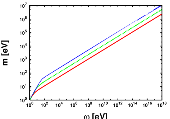
Figure 3: Upper bounds on $m$ in the scalar case, versus the photon energy $\omega$ in eV, for three values of external magnetic field $B=0.1,1,10$ Tesla, respectively from bottom to top.

Now we will restrict our analysis to the case of low energy photons, in particular between the optical and soft X-ray range, where the relevant scalar/pseudoscalar photon couplings can only be to photons and neutrinos. For neutrino masses of the order of meV the $\gamma\to\nu\bar{\nu}$ conversion process would be kinematically allowed and the $\Gamma$ appearing in Eq.(51) should be identified with the total width. Then, the formula for the absorption coefficient of the $\gamma\to\gamma\gamma$ process should be multiplied by the corresponding branching ratio. However, in the case of a PQ axion, the effects of axion couplings with neutrinos on the total width can be neglected due to the fact that axion-neutrino coupling is suppressed by neutrino masses. Indeed, the interaction Lagrangian in this case would be $L=g_{A}\bar{\nu}\gamma_{5}\nu\,\varphi_{A}$ where $\varphi_{A}$ is the axion field and $g_{A}\propto m_{\nu}/\Lambda$, while $\Lambda$ should be identified with the coupling $\Lambda_{P}$ appearing in Eq.(2).

Since we would like to generalize the results of our analysis to the PQ axion case, we restrict ourselves to the case where scalar/pseudoscalar particles are only effectively coupled to two photons. The total width will coincide in this case with the width in two photons given by

$$\Gamma=\frac{m^{3}}{64\pi\Lambda^{2}}\,.$$ (80)

The same expression, as a function of mass $m$ and coupling $\Lambda$, holds for both scalar and pseudoscalar interactions in Eqs.(1) and Eqs.(2). The fact the scalar/pseudoscalar particles are only coupled to photons greatly simplifies the analysis. In particular we can see that the expression for $\xi$ does not depend on the coupling $\Lambda$ and it is given by

$$\xi=\frac{1}{1024\,\pi^{2}}\frac{m^{12}}{|{\rm\vec{k}}|^{4}|{\rm\vec{B}}|^{4}\sin^{4}{\theta}}$$ (81)

where $|{\rm\vec{k}}|^{2}\simeq\omega^{2}-m^{2}$.

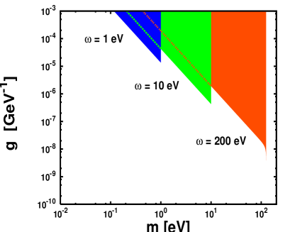
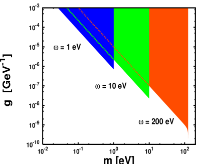
Figure 4: Excluded areas at 95 % C.L. in the ${\rm g}=1/\Lambda$ and $m$ plane, corresponding to photon energies $\omega=1$ eV (blue), $\omega=10$ eV (green), $\omega=200$ eV (red). We have assumed a magnetic field of 5 Tesla and $L=10$ m, a photon beam with momentum orthogonal to the direction of magnetic field ($\theta=\pi/2$) and number of photons per second $dN_{\gamma}/dt=10^{18}{\rm s}^{-1}$. Results for an integrated running time of one day and one year are shown in left and right plots respectively.

Now we consider a realistic experiment in which a monochromatic photon beam of frequency $\omega$ is traveling through a constant and homogeneous magnetic field of length $L$. If we choose the direction of polarization of the magnetic (electric) field component of the photon beam to be parallel to the external magnetic field, $\theta=\pi/2$, we select the maximum coupling for scalar (pseudoscalar) contributions. The main signal consists in photon pairs with different energies $\omega_{1}$ and $\omega_{2}$, restricted by the condition of energy conservation $\omega=\omega_{1}+\omega_{2}$. In the case in which $\omega\gg m$, the two photons are produced both almost forward and parallel to the original momentum of the photon beam, with a small opening angle $\delta\sim{\cal O}(m/\omega)\ll 1$. Then, excluded regions on the $(m-g)$ plane can be set, for instance, by requiring that no significant number of events are observed at 95% confidence level. Since this process has practically no background, due to the fact that in QED this effect is very suppressed, the corresponding significant number of standard deviation associated to a number of observed events $N_{S}$ would be of the order $\sqrt{N_{S}}$. In the particular case of 95% C.L. this implies $N_{S}\simeq 4$. Then, the requirement that no significant number of events are observed at 95% C.L. would imply

$$d_{\gamma}<\frac{4}{N_{\gamma}L}$$ (82)

where $d_{\gamma}$ is given in Eq.(51), with $\Gamma$ and $\xi$ given by Eqs.(80) and (81) respectively. For $N_{\gamma}$ we have assumed a representative laser brilliance corresponding to $dN_{\gamma}/dt=10^{18}/{\rm sec}$, as for instance in the case of free electron lasers.

Excluded regions in the $(m-g)$ plane corresponding to the upper limit in Eq.(82) are shown in Fig.4 for a magnetic field of 5 Tesla and for different values of photon beam energy, namely $\omega=1,~{}10,~{}200$ eV. Here in the left (right) plot we show the exclusion regions corresponding to one day (year) of running time, respectively. As we can see from these results, by increasing the photon energy, larger values of $\Lambda$ can be probed. In particular, with laser frequencies in the optical range $\omega=1$ eV, values of $\Lambda\raise 1.29167pt\hbox{$\;<$\kern-7.5pt\raise-4.73611pt\hbox{$\sim\;$}}10^{6}$ GeV can be explored after one year of running, while $\Lambda\raise 1.29167pt\hbox{$\;<$\kern-7.5pt\raise-4.73611pt\hbox{$\sim\;$}}10^{9}$ GeV can be reached with $\omega=200$ eV. The range of masses that can be explored with a 5 Tesla magnetic field, are just limited by the photon energy, namely $m\leq\omega$, for $\omega=1,10$ eV. However, for this value of the magnetic field and $\omega=200$ eV, the resonant region ($\xi\simeq 1$) is achieved below the kinematical upper bound $m\leq\omega$, and so for $\omega=200$ eV only the range of masses up to $m\raise 1.29167pt\hbox{$\;<$\kern-7.5pt\raise-4.73611pt\hbox{$\sim\;$}}125$ eV can be explored. Around the region close to the critical point, the $d_{\gamma}$ becomes insensitive to $\Lambda$ as shown in the previous section, see Eq.(58). This is the reason why the shape of the lower part of the red area, corresponding to $\omega=200$ eV, near the end point of $m$ is different from the other cases. The narrow width characterizing the end point region with large values of $\Lambda$, is of the order of $\Gamma$.

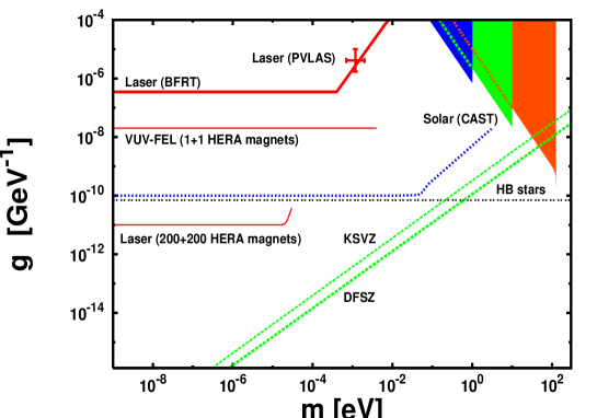
Figure 5: Results of right plot in Fig.4 embedded in the ${\rm g}=1/\Lambda$ and $m$ plane with exclusion regions coming from laser experiments BFRT [15] and PVLAS [17]. Exclusion regions coming from solar experiments searches for axion from the sun (Solar CAST) [29] and the horizontal branch stars (HB stars) [30] are also shown. The inclined lines (green) correspond to the predictions in DFSZ [31] and KSVZ [32] axion models. See text for further details.

Let us now discuss the consequences of these results for the axion physics. We remind here that the mass of the axion field connected to the PQ symmetry is related to the mass and decay constant of the pion by [4]

$$m_{A}=z^{1/2}/(1+z)\,m_{\pi}\,f_{\pi}/f_{A}=0.6\,{\rm meV}\times(10^{10}{\rm GeV}/f_{A})$$ (83)

where $f_{A}\gg 247$ GeV is the scale where this symmetry is broken, $f_{\pi}$ and $m_{\pi}$ are the decay constant and mass of the pion and the current quark mass ratio $z=m_{u}/m_{d}$. The couplings of the axion to SM particles are not only functions of the scale $f_{A}$, but also model dependent. For instance, the constant $f_{A}$ is connected to the photon coupling $g_{A\gamma}=\Lambda_{P}^{-1}$ in Eq.(2) by axial anomaly, and it is given by

$$g_{A\gamma}=-\frac{\alpha}{2\pi\,f_{A}}\left(\frac{E}{N}-\frac{2}{3}\frac{4+z}{1+z}\right)$$ (84)

where $E/N$ is the ratio of electromagnetic over color anomalies and it is model dependent. The most popular models are DFSZ [31], where axion is embedded in Grand Unified Theories, and KSVZ axion is the so called “hadronic” class of axions [32]. In both these models the couplings $g_{A\gamma}$ are predicted in terms of $f_{A}$ and are slightly different. The most stringent constraints on $g_{A\gamma}$ comes from cosmological and astrophysical arguments. However, there is a general class of experiments with laser that aim to produce axions in laboratory. They can be divided in two classes, one connected with photon-regeneration and another one that analyzes the indirect axion effects on light propagation. The first one is based on the Primakoff process [12], where a photon is converted in external magnetic field and then axions can be re-converted in photons with same mechanism after passing through a wall where all primary photons are stopped. The latter one probes the axion-coupling by measuring the change in the polarization of the photon after passing through magnetic field.

In Fig.5 we report the comparison between the present excluded areas in the $(m-g)$ plane in the case of axion searches, by embedding the results contained in the right plot of Fig.4 corresponding to one year of integrated running time. The predictions of the models of DFSZ and KSVZ axions are also shown. The exclusion regions based on the solar experiments for axions from the Sun [29] (indicated with Solar (CAST) = CERN Axion Solar Telescope) and the constraints from horizontal branch (HB) stars [30] arising from a consideration of stellar energy losses through axion production are reported. Recently, the PVLAS experiment [17], reported the observation of a rotation of the polarization plane of light propagating through a transverse static magnetic field. This is shown as a point with error bars on the border of laser area in Fig.5. Notice that the signal seen in [17] is incompatible with the exclusion area from experiment [15]. Constraints coming from the galactic dark matter experiments [33] are not reported in Fig.5. However, this class of experiments strongly constrain only a narrow region in the $(m-g)$ plane corresponding to axion masses in the range $10^{-6}{\rm eV}\raise 1.29167pt\hbox{$\;<$\kern-7.5pt\raise-4.73611pt\hbox{$\sim\;$}}m_{a}\raise 1.29167pt\hbox{$\;<$\kern-7.5pt\raise-4.73611pt\hbox{$\sim\;$}}10^{-5}{\rm eV}$. We have also included the results of a recent proposal [18, 19] of laser experiment based on high-energy photon regeneration mechanisms, which is the X-ray analogous of the optical one. The free-electron lasers (FEL) at DESY’s TESLA and dipole magnets of the type used in DESY’s electron-proton collider HERA have been employed. The two horizontal lines correspond to the experimental analysis based on 1+1 and 200+200 HERA dipole magnets.

As clear from the plot, the new areas in the $(m-g)$ plane that can be probed by searching for photon splitting in two photons would allow to cover complementary areas not achievable by other two classes of laser experiments. It is worth noticing that both the predictions of KSVZ and DFSZ models fall inside the area that could be probed by the $\omega=200$ eV laser experiment proposed here. As we can see from these results, the astrophysical constraints rule out a large region of the parameter space including the one we are interested in, as well as the region covered by laser experiments. However, recently it has been shown that in certain models these astrophysical constraints can be evaded [34].

Finally, we would like to emphasize that in the case in which a significant number of events of photon splitting $\gamma\to\gamma\gamma$ should be found, the values of the scalar/pseudoscalar mass and width can be easily reconstructed. This would allow to precisely tune the external magnetic field and photon energy in order to approach the resonant region, where the effect of photon splitting could be largely amplified. Regarding the origin of the interaction, if there is a scalar or pseudoscalar coupling, this can be disentangled by analyzing the polarization of the final photons with respect to the direction of the magnetic field or by analyzing their angular distributions, provided that a sufficient number of events are observed.

Let us also shortly discuss the case of the Higgs boson effects in this context. We start with the case of high energy photon beam traveling in a constant magnetic field and with the coupling to a light Higgs boson of mass $m_{H}\simeq 120$ GeV. The main decay mode of the Higgs in this scenario is in $b\bar{b}$. In the effective propagator there would be a very light mode, and a massive mode of the size of the Higgs mass. In order to generate the $\gamma\to b\bar{b}$ decay in external field one needs first to check if the condition (36) is satisfied for the corresponding massive mode. As we discussed in the previous sections this would require too high critical magnetic fields, when the energy of the photon beam is of the order of TeV, which cannot be realized in the laboratory. Nevertheless, there might be the possibility of a sizeable effect on the photon splitting mediated by the Higgs effective coupling in the framework of astrophysics, for example in the core of a supernova, where magnetic fields are very large. However, in that case the approximation of considering only constant and homogeneous magnetic fields is not correct, since also plasma effects should be taken into account. When magnetic fields are inhomogeneous, momentum can be absorbed and the Higgs boson could in principle be produced on-shell by means of the Primakoff process. Although the analysis of this latter effect in astrophysical context should be quite interesting, it goes beyond the scope of the present paper.

6 Conclusions

In this paper we have investigated the analytical properties of the effective photon propagator in an external homogeneous and static magnetic or electric fields, in the presence of scalar/pseudoscalar couplings. These results have been obtained by summing up in the photon propagator the relevant class of Feynman diagrams. They include the ones with mixing term of photon with scalar/pseudoscalar fields, where in the scalar/pseudoscalar propagator the corresponding self-energies have been exactly summed up. Then, we analyzed the solutions of the associated dispersion relations.

Due to the presence of an external field, the standard photon dispersion relations in vacuum will be modified. While the effect of the real part of scalar/pseudoscalar self-energy can be re-absorbed in the corresponding mass term of the scalar/pseudoscalar, the imaginary part, connected to the corresponding width $\Gamma$, could play a crucial role in the photon dispersion relations giving rise to a non-vanishing contribution to the imaginary part of the effective photon propagator. In other words, the presence of $\Gamma$ can induce a non-vanishing contribution for photon absorption coefficient.

As known, two new propagation modes are allowed for the photon, in addition to the usual one which is not affected by the external field contributions. The lightest one is associated to a light-like mode with refraction index $n>1$, while the heaviest one corresponds to a massive mode with mass of the order of the scalar/pseudoscalar one.

The new aspect of our work with respect to previous studies concerns the inclusion of the effects of the imaginary part of scalar/pseudoscalar self-energy in the effective photon propagator. In particular, we have shown that the massive mode can be allowed only when the contributions of the scalar/pseudoscalar width $\Gamma$ are smaller or comparable to the mixing effects, see Eq.(36). This will give rise to a critical condition for the external field, which is absent in the limit $\Gamma\to 0$, depending on the photon energy, scalar/pseudoscalar masses and the two-photon coupling. A finite width for the photon can then be induced for the massive mode, being proportional to $\Gamma$, generating a non-vanishing value for the photon absorption coefficient $d_{\gamma}$.

Although very small, being suppressed by the scalar/pseudoscalar width, the $d_{\gamma}$ can be sizeably enhanced due to a strong resonant phenomenon. In particular, we have found that a potentially large contribution to the splitting conversion $\gamma\to\gamma\gamma$ could be generated from the scalar/pseudoscalar decay in two photons when the external field approaches its critical value.

We have also analyzed the contribution to the absorption coefficient induced by the massless photon mode. In the case of an external magnetic field and a scalar interaction, we find that the probability of photon splitting in two photons turn out to be very small, being suppressed by $({\rm B}/{\rm B_{cr}})^{6}$ where (in relativistic unities) ${\rm B_{cr}}=m\Lambda$. Nevertheless, this effect, depending on mass $m$ and coupling $\Lambda$, could be much larger than the one induced by the QED vacuum polarization in the presence of an external magnetic field. For instance, for characteristic values of $m=10^{-3}$eV and $\Lambda=10^{6}$GeV, we find that $d_{\gamma}$ is about five order of magnitude larger than the corresponding QED one. The leading contribution to $d_{\gamma}$ is provided by the small effects of dispersions in the refraction index. For the case of a pseudoscalar interaction, due to the parity violating coupling and kinematic factors, the photon splitting induced by the massless mode is forbidden.

We have analyzed the consequences of these results for a new kind of laser laboratory experiments, based on the searching of the photon splitting $\gamma\to\gamma\gamma$ conversion in external constant and homogeneous magnetic field. In particular, we have considered the photon splitting phenomenon induced by the massive mode. By taking the case of high brilliance lasers with $dN_{\gamma}/dt=10^{18}$/sec, in the range between optical ($\omega\simeq 1\,{\rm eV}$) and the low X-ray ($\omega\simeq 200$ eV) frequencies, magnetic fields of 10 meters long and of the order of 5 Tesla, we show that it is possible to probe a large area of the $m$ and $g=1/\Lambda$ plane, provided that the process $\gamma\to\gamma\gamma$ can be efficiently detected. The probed areas for scalar and pseudoscalar case are slightly different. We find that in the case of $\omega\simeq 200$ eV, scalar/pseudoscalar masses can be probed up to $m<100$ eV , while in the case of $\omega=1$ eV the region up to the maximum value allowed by the energy conservation, i.e. $m<1$ eV can be explored. Moreover, the sensitivity on the scale $\Lambda$ associated to the two-photon coupling can become , in one year of running time, close to $\Lambda\simeq 10^{6}$ GeV and $\Lambda\simeq 10^{9}$ GeV, corresponding to the case of $\omega=1$ eV and $\omega=200$ eV laser frequencies, respectively.

We have also compared our results with the present bounds from axion searches. In particular, by restricting our predictions to the case of pseudoscalar couplings, we found that a large area in the $m$ and $g$ plane of the axion can be tested. Remarkably, this area is complementary to the ones already explored by the present laser experiments, like PVLAS and BFRT, and to the sensitivity area of new recent proposal based on the photon-regeneration class of experiments with X-ray free electron laser facility at HERA. We have also shown that some predictions of the KSVZ and DFSZ models could be tested by means of $\gamma\to\gamma\gamma$ searches in external magnetic fields.

Acknowledgments
We would like to acknowledge useful discussions with D. Anselmi, M. Chaichian, M. Giovannini, G.F. Giudice, K. Kajantie, B. Mele, P.B. Pal, R. Rattazzi, P. Sikivie, L. Stodolsky, and K. Zioutas. E.G. would like to thank the CERN TH-division for kind hospitality during the preparation of this work. S.R. thanks the ASICTP for kind hospitality during the final stages of this work. This work is supported by the Academy of Finland (Project number 104368).

Appendix A

In this appendix we report the exact solutions of the mass-gap equation (26). This is a cubic algebraic equation and can be analytically solved by using the known cubic formula. In particular, by substituting $k^{2}=m^{2}+\varepsilon$ in Eq. (26), this can be simplified as

$$x^{3}+x^{2}+x\left(\xi_{\Gamma}-\xi_{\Delta}\right)+\xi_{\Gamma}=0\,,$$ (85)

where $x=\varepsilon/m^{2}$, $\xi_{\Gamma}=\Gamma^{2}/m^{2}$ and $\xi_{\Delta}=\Delta/m^{4}$. Notice that in writing the gap equation we have identified the ${\rm Im}\Sigma(k^{2})$ with $-m\Gamma$. In general this statement is not correct since the imaginary part of scalar/pseudoscalar width depends on $k^{2}$, in particular for the photon splitting it is proportional to $(k^{2})^{2}/\Lambda^{2}$, see Appendix B for more details. However, the approximation to set ${\rm Im}\Sigma(k^{2})=-m\Gamma$ is valid only when $k^{2}\sim{\cal O}(m^{2})$, that is for the massive solutions. On the other hand, for the massless mode where, $k^{2}\sim{\cal O}(\Delta/m^{2})$, the ${\rm Im}\Sigma(k^{2})$ can be neglected with respect to the $m^{2}$ term and one can safely switch off the ${\rm Im}\Sigma(k^{2})$ in the scalar/pseudoscalar propagator provided that $\Delta/m^{4}\ll 1$. Therefore, in order to simplify the problem, one can solve the gap equation by using ${\rm Im}\Sigma(k^{2})=m\Gamma$ and then, in order to recover the correct result for the massless mode, set $\xi_{\Gamma}\to 0$ on the corresponding massless solution.

By using this approach, we solve the cubic equation above and find the following expressions for the solutions of Eq. (26), namely $k^{2}=M^{2}_{0}$ and $k^{2}=M^{2}_{\pm}$ with

$$M^{2}_{0} = \lim_{\xi_{\Gamma}\to 0}\,m^{2}\left(\frac{2}{3}+X_{+}+X_{-}\right)$$

$$M^{2}_{\pm} = m^{2}\left(\frac{2}{3}-\frac{1}{2}\left(X_{+}+X_{-}\right)\pm i\frac{\sqrt{3}}{2}\left(X_{+}-X_{-}\right)\right)\,,$$ (86)

where

$$X_{\pm}=\left(R\pm\sqrt{D}\right)^{1/3},~{}~{}~{}~{}~{}~{}D=Q^{3}+R^{2}$$ (87)

and in our case

$$Q=\frac{3\left(\xi_{\Gamma}-\xi_{\Delta}\right)-1}{9},~{}~{}~{}~{}~{}~{}~{}R=-\frac{9\left(2\xi_{\Gamma}+\xi_{\Delta}\right)+2}{54}\,.$$ (88)

The massive solutions $k^{2}=M_{\pm}^{2}$ are real only when the condition $D<0$ is satisfied, where

$$D=\frac{1}{108}\left\{-\xi_{\Delta}^{2}+4\,\xi_{\Gamma}-4\,\xi_{\Delta}^{3}+20\,\xi_{\Delta}\,\xi_{\Gamma}+12\,\left(\xi_{\Delta}^{2}\,\xi_{\Gamma}-\xi_{\Gamma}^{2}\,\xi_{\Delta}\right)+8\,\xi_{\Gamma}^{2}+4\,\xi_{\Gamma}^{3}\right\}\,.$$ (89)

In our problem, the parameters $\xi_{\Delta}\ll 1$ and $\xi_{\Gamma}\ll 1$ are very small quantities. We remind here that these are proportional to inverse powers of the effective coupling $\Lambda$ with two photons, which is assumed to be much larger than the typical scales appearing in the numerator of $\xi_{\Gamma}$ and $\xi_{\Delta}$, namely the photon energy $\omega$, momentum $\vec{k}$, and external field. From a first inspection of Eq.(89), one can see that, in order to have real solutions ($D<0$), these parameters should satisfy the following hierarchy $\xi_{\Gamma}\sim\xi_{\Delta}^{2}$. This is also consistent with the fact that $\xi_{\Gamma}$ and $\xi_{\Delta}$ scale as $\xi_{\Gamma}\sim 1/\Lambda^{4}$ and $\xi_{\Delta}\sim 1/\Lambda^{2}$ respectively as a function of $\Lambda$. In particular, by dropping the terms of order ${\cal O}(\xi_{\Delta}^{3})$ in Eq.(89), the condition $D<0$ is equivalent to

$$\xi_{\Delta}>\xi_{\Delta}^{\rm c\,(0)}\equiv 2\sqrt{\xi_{\Gamma}}\,$$ (90)

which is exactly the inequality in (36) derived under the approximation of neglecting terms of order $\xi_{\Delta}^{3}$.

There is only one solution of $D=0$, corresponding to real and positive values of $\xi_{\Delta}$ and $\xi_{\Gamma}$, and it is given by

$$\xi_{\Gamma} = \xi_{\Delta}-\frac{2}{3}+\frac{2\left(1-27\xi_{\Delta}\right)}{3H(\xi_{\Delta})}+\frac{H(\xi_{\Delta})}{6}\,,$$ (91)

where the expression for the function $H(x)$ is

$$H(x) = \left(8+540x-729x^{2}+3\,\sqrt{3}\,\sqrt{x}\left(8+27x\right)^{3/2}\right)^{1/3}\,.$$ (92)

As we can see from these results, there always exists a critical value for the external fields for which the massive solutions become degenerate, implying the appearance of a double pole in the effective photon propagator.

Now we will provide below the corresponding solutions obtained by expanding the exact ones in terms of the small parameters $\xi_{\Delta}$ and $\xi_{\Gamma}$. Let us first define $\xi_{\Delta}^{\rm c}$ being the value of $\xi_{\Delta}$ satisfying the exact solution of Eq.(91). Then, by expanding $\xi_{\Delta}$ in powers of $\delta=\Gamma/m$, we obtain, up to terms ${\cal O}(\delta^{6})$, the following expression

$$\xi_{\Delta}^{\rm c}=\xi_{\Delta}^{\rm c\,(0)}\,\Big{(}1+R(\delta)\,\Big{)}$$ (93)

where

$$R(x)=x-\frac{1}{2}\,x^{2}+x^{3}-\frac{5}{2}\,x^{4}+8\,x^{5}+{\cal O}(x^{6})\,.$$ (94)

Finally, the corresponding next-to-leading order corrections, in $\xi_{\Delta}$ expansion, to the solutions in Eqs.(30) are given by

$$M_{0} = -\frac{\Delta}{m^{2}}\left(1-\xi_{\Delta}+2\xi_{\Delta}^{2}\right)$$

$$M^{2}_{\pm} = m^{2}\left\{1+\frac{\xi_{\Delta}}{2}\left(1\pm\sqrt{1-\xi}\right)-\frac{\xi_{\Delta}^{2}}{2}\left(1\pm\frac{2-\xi}{2\sqrt{1-\xi}}\right)\right\}$$ (95)

where the symbol $\xi=4\xi_{\Gamma}/\xi_{\Delta}^{2}$ is the same as appearing in Eq.(31). Notice that for the solutions in (95) the range $0<\xi<1$ is not valid anymore, and, according to Eq.(93), must be modified as $0\leq\xi\leq 1-\delta+{\cal O}(\delta^{2})$. It can be easily checked that for the maximum value $\xi^{\rm max}=1-\delta$, the difference $M^{2}_{+}-M^{2}_{-}$ vanishes up to terms of order ${\cal O}(\xi_{\Delta}^{3})$, within the validity of the approximated solutions.

Regarding the massless mode, the expression for $M_{0}^{2}$ can be easily re-obtained by setting to zero the scalar/pseudoscalar width $\Gamma$ directly in the gap equation. This will reduce the cubic equation in Eq.(26) to a second order one. In particular, by setting ${\rm Im}\Sigma(k^{2})$ to zero in Eq.(26), one gets a more compact solution for the massless mode, equivalent to the first solution in Eq.(86), given by

$$M_{0}^{2}=\frac{m^{2}}{2}\left(1-\sqrt{1+4\xi_{\Delta}}\right)\,,$$ (96)

where the leading orders in $\xi_{\Delta}$ expansion easily recover the corresponding results in Eqs.(30) and (95).

Appendix B

In this appendix we provide the calculation at 1-loop of the imaginary part of scalar (pseudoscalar) self-energy $\Sigma_{S(P)}$, induced by the interactions in Eqs.(1),(2). While the real part of $\Sigma_{S(P)}$ is divergent, its imaginary part is finite at 1-loop and can be easily calculated by making use of the optical theorem. In particular, the ${\rm Im}[\Sigma_{S(P)}(k^{2})]$ is connected to the square modulus of the off-shell scalar/pseudoscalar decay in two on-shell photons, which schematically can be represented as

(97)

where $Z$ is the renormalization constant of scalar/pseudoscalar field, the continuous and dashed line stands for the scalar/pseudoscalar and photon fields respectively, and $k,k_{1,2}$ are the corresponding momenta. In the left-hand side of (97), the vertical dashed lines correspond to the Cutkosky rule which selects the imaginary part of the photon propagators in the loop, by replacing in each of them $1/(p^{2}+i\epsilon)\to-\pi\delta(p^{2})\theta(\omega)$, with $p^{2}\equiv p_{\mu}p^{\mu}$ and $\omega\equiv p_{0}$, where $p_{\mu}$ indicate the generic 4-momenta of photon lines in the loop. The factor $1/2$ in front of the amplitude square is due to symmetry factor connected to the two photon lines. By using the Cutkosky rule and the fact that at this order in perturbation theory $Z=1$, one obtains

$${\rm Im}[\Sigma_{S(P)}(k^{2})] = -\frac{1}{2}\frac{d^{3}k_{1}}{(2\pi)^{3}2\omega_{1}}\frac{d^{3}k_{2}}{(2\pi)^{3}2\omega_{2}}(2\pi)^{4}\delta^{4}(k-k_{1}-k_{2})\,\sum_{\rm pol}\,\left|V_{\gamma\gamma}^{S(P)}(k_{1},k_{2})\right|^{2}$$ (98)

where $V_{\gamma\gamma}^{S(P)}(k_{1},k_{2})$ is the two photon vertex for the scalar(pseudoscalar) field given in Eq.(55), and the $k_{1,2}$ are the corresponding final photon momenta on shell, $k_{1,2}^{2}=0$. The sum $\sum_{\rm pol}$ is extended to all photon polarizations. Notice that, as an approximation, we have not considered the effect of the external field corrections, and so the photon dispersion relations are not modified.

Finally, by using the results in Eq.(55), we get, for the contribution at 1-loop to the self-energy,

$${\rm Im}[\Sigma_{S(P)}(k^{2})]=-\frac{(k^{2})^{2}}{64\pi\Lambda^{2}_{S(P)}}\,.$$ (99)

When Eq.(98) is evaluated on-shell the scalar(pseudoscalar) width $\Gamma_{S(P)}$ on-shell is recovered by means of the relation ${\rm Im}[\Sigma(k^{2})]|_{k^{2}=m^{2}}=-m\Gamma$, in particular

$$\Gamma_{S(P)}=\frac{m^{3}}{64\pi\Lambda^{2}_{S(P)}}\,,$$ (100)

which is in agreement with Eq.(80).

References

- [1] S. Dawson, J.F. Gunion, H.E. Haber, and G. Kane, The Higgs Hunter’s Guide (1989); For a recent review on Higgs physics, see A. Djouadi, hep-ph/0503172.
- [2] J.P. Leveille, Phys. Lett. 38 B, 123 (1979); 88B, 395 (E) (1979); R.N. Cahn, M.S. Chanowitz and N. Fleishon, Phys. Lett. 82B, 395 (1979); J. Ellis, M.K. Gaillard, and D.V. Nanopoulos, Nucl. Phys. B106, 292 (1976); A.I. Vainshtein, M.B. Voloshin, V.I. Zakharov, and M.A. Shifman, Sov. J. Nucl. Phys. 30, 711 (1979); L. Bergstrom and G. Hulth, Nucl. Phys. B259, 137 (1985); B276, 744 (E) (1986); A. Barroso, J. Pulido, and J.C. Romão, Nucl. Phys. B267, 509 (1986); E. Gabrielli, V.A. Ilyin, and B. Mele, Phys. Rev. D 56 5945 (1997), D58 119902(E) (1998): A.T. Banin, I.F. Ginzburg, and I.P. Ivanov, Phys. Rev. D59 115001 (1999).
- [3] R.D. Peccei and H. R. Quinn, Phys. Rev. Lett. 38, 1440 (1977) and Phys. Rev. D16, 1791 (1977).
- [4] S. Weinberg, Phys. Rev. Lett. 40, 223 (1978); F. Wilczek, Phys. Rev. Lett. 40, 279 (1978); M. Dine, W. Fischler, and M. Srednicki, Phys. Lett. B104, 199 (1981).
- [5] G.Raffelt, Stars as Laboratories for Fundamental Physics, (The University of Chicago Press), 1996.
- [6] R. Barate et al., Phys. Lett. B565, 61 (2003).
- [7] Eidelman S et al., Particle Data Group Collaboration, 2004 , Phys. Lett. B 592, 1 (2004).
- [8] For a recent review on axion phenomenology see, P. Sikivie, Proceedings of the 11th Int. Symposium on Particles, Strings and Cosmology (PASCOS 2005), AIP Conf. Proc. 805: 23-29,2006; hep-ph/0509198
- [9] P. Sikivie, Phys. Rev. Lett. 51, 1415 (1983); Erratum-ibid. 52, 695 (1983); Ibid. Phys. Rev. D 32 (1985) 2988; J.N. Clarke, G. Karl, and P.J.S. Watson, Can. J. Phys. 60, 1561 (1982).
- [10] M. Gasperini, Phys. Rev. Lett. 59, 396 (1987); D. Harari and P. Sikivie, Phys. Lett. B289, 67 (1992); G. Raffelt and L. Stodolsky, Phys. Rev. D 37, 1237 (1998); C. Csáki, N. Kaloper, J.Terning, Phys. Rev. Lett. 88, 161302 (2002); Y. Grossman, S. Roy, and J. Zupan, Phys. Lett. B543, 23 (2002); P. Jain, S. Panda and S. Sarala, Phys. Rev. D 66, 085007 (2002); M. Christensson and M. Fairbairn, Phys. Lett. B565, 10 (2003); E. Mortsell and A. Goobar, JCAP 0304, 003 (2003); S. Das, P. Jain, J. P. Ralston, and R. Saha, JCAP 0506, 002 (2005).
- [11] G. Raffelt Phys. Rev. D 33, 897 (1986); G. Raffelt and D. S. Dearborn, Phys. Rev. D 37, 549(1988); G. Raffelt. Phys. Rept. 198, 1 (1990); M. S. Turner, Phys. Rept. 197, 67 (1990).
- [12] H. Primakoff, Phys. Rev. 81, 899 (1951).
- [13] K. van Bibber, P. McIntyre, D. Morris, and G. Raffelt, Phys. Rev. D 39, 2089 (1989).
- [14] K. Van Bibber, N.R. Dagdeviren, S.E. Koonin, A. Kerman, H.N. Nelson, Phys. Rev. Lett. 59, 759 (1987).
- [15] R. Cameron et al., Phys. Rev. D47, 3707 (1993).
- [16] L. Maiani, R. Petronzio, and E. Zavattini, Phys. Lett. B175, 359 (1986).
- [17] E. Zavattini et al., PVLAS Collaboration, hep-ex/0507107.
- [18] A. Ringwald, Proceedings of the 9th Int. Conference on Astroparticle and Underground Physics (TAUP 2005), Zaragoza, Spain, 10-14 Sep 2005, hep-ph/0511184.
- [19] R. Rabadan, A. Ringwald, and K. Sigurdson, hep-ph/0511103.
- [20] A.K. Ganguly, S. Konar, P.B. Pal, Phys. Rev. D60, 105014 (1999); J.C. D’Olivo, J.F. Nieves, and Sarira Sahu, Phys. Rev. D67, 025018 (2003).
- [21] S. L. Adler, Ann. Phys. (N.Y.) 67, 599 (1971).
- [22] J. Toll, unpublished Ph.D. dissertation, Princeton University, Princeton, N.J. (1952); N. P. Klepikov, Zh. Eksp. Teor. Fiz. 26, 19 (1954); for discussion of dispersive effects, see also: A. Minguzzi, Nuovo Cimento 6, 501 (1957) and 9 (1958), 145; J. J. Klein and B. P. Nigam, Phys. Rev. B135, 1279 (1964).
- [23] T. Erber, Rev. Mod. Phys. 38, 626 (1966); W.Y. Tsai and T. Erber, Phys. Rev. D 10, 492 (1974).
- [24] N.V. Mikheev, A. Ya. Parkhomenko, and L.A. Vassilevskaya, Phys. Rev. D 60, 035001 (1999).
- [25] Sh. Zh. Akhmadaliev et al., Phys. Rev. Lett. 89, 061802 (2002)
- [26] W. Heisenberg and H. Euler, Z. Phys. 38, 714 (1936).
- [27] I.F. Ginzburg, G.L. Kotkin, V.G. Serbo, and V.I. Telnov, Nucl. Phys. Instrum. methods Phys. Res. 205, 47 (1983); I.F. Ginzburg, G.L. Kotkin, S.L. Panfil, V.G. Serbo, and V.I. Telnov, Nucl. Instrum. Methods Phys. Res. A 294, 72 (1990).
- [28] Proceedings of the Worldwide study on Physics and Expriments with future linear colliders (Ed. by E. Fernández and A. Pacheco), Vol. II, April 28 - May 5, 1999, Sitges, Barcelona; A. Sopczak, hep-ph/0502002; P. Garcia-Abia, W. Lohmann, A. Raspereza, hep-ex/0505096.
- [29] K. Zioutas et al., Cast Collaboration, Phys. Rev. Lett. 94 121301. (2005).
- [30] G. Raffelt Ann. Rev. Nucl- part. Sci. 49, 163 (1999).
- [31] A.R. Zhitnitsky, Sov. J. Nucl. Phys. 31, 260 (1980); M. Dine and W. Fischler, Phys. Lett. B120, 137 (1983).
- [32] J.E. Kim, Phys. Rev. Lett. 43, 103 (1979); M.A. Shifman, A.I. Vainstein, and V.I. Zakharov, Nucl. Phys. B166, 493 (1980).
- [33] See references cited in [7] for more details.
- [34] E. Masso and J. Redondo, JCAP 0509, 015 (2005); P. Jain and S. Mandal, astro-ph/0512155.