X(1812) in Quarkonia-Glueball-Hybrid Mixing Scheme

Xiao-Gang He^1,2, Xue-Qian Li¹, Xiang Liu¹ and Xiao-Qiang Zeng¹

¹Department of Physics, Nankai University, Tianjin

²NCTS/TPE, Department of Physics, National Taiwan University, Taipei

Recently a $J^{PC}=0^{++}$ ($X(1812)$) state with a mass near the threshold of $\omega$ and $\phi$ has been observed by the BES collaboration in $J/\psi\to\gamma\omega\phi$ decay. It has been suggested that it is a $I^{G}=0^{+}$ state. If it is true, this state fits in a mixing scheme based on quarkonia, glueball and hybrid (QGH) very nicely where five physical states are predicted. Together with the known $f_{0}(1370)$, $f_{0}(1500)$, $f_{0}(1710)$, and $f_{0}(1790)$ states, $X(1812)$ completes the five members in this family. Using known experimental data on these particles we determine the ranges of the mixing parameters and predict decay properties for $X(1812)$. We also discuss some features which may be able to distinguish between four-quark and hybrid mixing schemes.

PACS numbers: 12.39.Mk, 13.25.Gv

1 Introduction

An enhancement has been observed by the BES collaboration near the threshold of the invariant mass spectrum of $\omega\phi$ in the radiative decay $J/\psi\rightarrow\gamma\omega\phi$. Their results indicate the existence of a new resonant state of $J^{PC}=0^{++}$ with a mass and a width given by $m=1812^{+19}_{-26}(\mathrm{stat})\pm 18(\mathrm{syst})\mathrm{MeV}/\mathrm{c}^{2}$ and $\Gamma=105\pm 20(\mathrm{stat})\pm 28(\mathrm{syst})\mathrm{MeV}/\mathrm{c}^{2}$. The observed branching ratio for $J/\psi\to\gamma\omega\phi$ is $B(J/\psi\rightarrow\gamma X)\cdot B(X\rightarrow\omega\phi)=(2.61\pm 0.27(\mathrm{stat})\pm 0.65(\mathrm{syst}))\times 10^{-4}$ [1]. This resonant state is named as $X(1812)$.

Earlier the BES collaboration also reported another $J^{PC}=0^{++}$ state in the spectrum of $\pi\pi$ of $J/\psi\to\phi\pi\pi$ with a mass of $1790^{+40}_{-30}$ MeV and a width of $270^{+80}_{-30}$ MeV, named $f_{0}(1790)$. The branching ratio $B(J/\psi\to\phi f_{0}(1790)\to\phi\pi\pi)$ is determined to be $(6.2\pm 1.4)\times 10^{-4}$[2]. It has been suggested that $f_{0}(1790)$ is a $I^{G}(J^{PC})=0^{+}(0^{++})$ state. There are several other $0^{+}(0^{++})$ states with mass in the range of 1 GeV to 2 GeV, these are $f_{0}(1370)$ , $f_{0}(1500)$ and $f_{0}(1710)$. The states $f_{0}(1370)$, $f_{0}(1500)$, $f_{0}(1710)$, $f_{0}(1790)$, having the same quantum numbers with masses not far from each other, can have significant mixing. The usual basis describing meson mixing based on QCD picture, includes quarkonia and glueball. Without considering excited states, the ground states of the quarkonia and glueball basis, $N=(\bar{u}u+\bar{d}d)/\sqrt{2}$, $S=\bar{s}s$ and $G=gg$, can only accommodate three $0^{+}(0^{++})$ states. Previous studies have, therefore, considered three states mixing with $f_{0}(1370)$, $f_{0}(1500)$ and $f_{0}(1710)$ as members[3, 4, 5, 6]. The addition of $f_{0}(1790)$ into the picture requires an enlargement of the basis. In QCD, the next simplest states having the quantum numbers compared with the quarkonia and glueball basis is the hybrid basis composed of an anti-quark $\bar{q}$, a quark $q$ and a gluon $g$, i.e. $\bar{q}qg$ which contains two independent $0^{+}$ states, $\xi_{N}=(\bar{u}u+\bar{d}d)g/\sqrt{2}$ and $\xi_{S}=\bar{s}sg$. Therefore introduction of hybrid states to accommodate $f_{0}(1790)$ implies the existence of another $0^{+}$ state. In our recent study[7], we have carried out such an analysis. Since the mass of the possible new state was not known at the time, two solutions for the eigenstates (mainly hybrid states) were obtained with one of them having a mass about 1760 MeV and the other about 1820 MeV. The later case fits the new $X(1812)$ state well within the experimental error.

We remark that the identification of $X(1812)$ as a mainly hybrid state has an extra bonus. If $X(1812)$ is a quarkonia state, $J/\psi\rightarrow\gamma\omega\phi$ decay is a doubly OZI suppressed process. Thus its branching ratio should be small. The observed branching ratio $B(J/\psi\rightarrow\gamma X)\cdot B(X\rightarrow\omega\phi)=(2.61\pm 0.27(\mathrm{stat})\pm 0.65(\mathrm{syst}))\times 10^{-4}$ is too large to be explained. This fact indicates that $X(1812)$ contains exotic component which allows larger branching ratio for $J/\psi\to\gamma X(1812)\to\gamma\omega\phi$. We note that both glueball and hybrid states can transit into a $\omega\phi$ state without the usual OZI suppression. If indeed $X(1812)$ is mainly a hybrid state, it can naturally explain the large than expected branching ratio for $J/\psi\to\gamma X(1812)\to\gamma\omega\phi$. The quarkonia, glueball and hybrid (QGH) mixing scheme proposed in Ref. [7] therefore provides a natural description of the five members in the $0^{+}(0^{++})$ family mentioned above. In this paper we study further the implications of the QGH mixing scheme, and comment on four quark scheme for $X(1812)$.

2 A Scenario for QGH mixing matrix

We now study possible structure for the QGH mixing. The effective Hamiltonian $\mathcal{H}$ for the system cannot be calculated from QCD yet because of complicated non-perturbative effects. There have been some efforts to estimate the masses of hybrid mesons by using Constituent Gluon Model[8], Flux Tube Model[9], Bag Model[10], QCD Sum Rules[11] and also Lattice QCD[12]. A summary at HARDRON’95 listed the mass range for the ground-state of hybrid as 1.3-1.8GeV[13]. Some relevant topics about the experimental status of hybrid states can be found in Ref.[14]. In Ref.[15], the author used the bag model to estimate the mass ranges of scalar hybrids, and obtained 1.51-1.90 GeV for $(u\bar{u}+d\bar{d})g/\sqrt{2}$ and 2.0-2.1 GeV for $s\bar{s}g$. Lattice calculations give $M_{G}$[16] to be in the range $1.5\sim 1.7$ GeV. Since theoretical uncertainties on the masses are too large to rule out a particular mass range, we will take a more phenomenological approach assuming the QGH mixing scheme and study some consequences of this mixing scheme. Although it is difficult to have a precise theoretical prediction on the mixing parameters, some simplifications can be made. One first notices that the matrix elements $<N|\mathcal{H}|S>$ and $<\xi_{N}|\mathcal{H}|\xi_{S}>$ are OZI suppressed and can therefore be neglected at the lowest order approximation. The same argument applies to $<N,S|\mathcal{H}|\xi_{N,S}>$. Possible large mixing can occur between glueball and quarkonia, hybrid states. Since the couplings of glueball-quarkonia, and glueball-hybrid are flavor-independent, one has the relation $e=\langle G|\mathcal{H}|\xi_{S}\rangle=\langle G|\mathcal{H}|\xi_{N}\rangle/\sqrt{2}$, and $f=\langle G|\mathcal{H}|S\rangle=\langle G|\mathcal{H}|N\rangle/\sqrt{2}$. With the approximation described above, the mass matrix can be expressed as

$$M=\left(\begin{array}[]{ccccc}M_{\xi_{S}}&0&e&0&0\\ 0&M_{\xi_{N}}&\sqrt{2}e&0&0\\ e&\sqrt{2}e&M_{G}&f&\sqrt{2}f\\ 0&0&f&M_{S}&0\\ 0&0&\sqrt{2}f&0&M_{N}\end{array}\right),$$ (6)

where $M_{\xi_{S}}=\langle\xi_{S}|\mathcal{H}|\xi_{S}\rangle$, $M_{\xi_{N}}=\langle\xi_{N}|\mathcal{H}|\xi_{N}\rangle$, $M_{G}=\langle G|\mathcal{H}|G\rangle$, $M_{S}=\langle S|\mathcal{H}|S\rangle$ and $M_{N}=\langle N|\mathcal{H}|N\rangle$.

We parameterize the relation between the physical states and the basis as

$$\left(\begin{array}[]{c}|X_{1}\rangle\\ |X_{2}\rangle\\ |X_{3}\rangle\\ |X_{4}\rangle\\ |X_{5}\rangle\end{array}\right)=\left(\begin{array}[]{c}|X(1812)\rangle\\ |f_{0}(1790)\rangle\\ |f_{0}(1710)\rangle\\ |f_{0}(1500)\rangle\\ |f_{0}(1370)\rangle\end{array}\right)=U\left(\begin{array}[]{c}|\xi_{S}\rangle\\ |\xi_{N}\rangle\\ |G\rangle\\ |S\rangle\\ |N\rangle\end{array}\right),\;\;U=\left(\begin{array}[]{ccccc}v_{1}&w_{1}&z_{1}&y_{1}&x_{1}\\ v_{2}&w_{2}&z_{2}&y_{2}&x_{2}\\ v_{3}&w_{3}&z_{3}&y_{3}&x_{3}\\ v_{4}&w_{4}&z_{4}&y_{4}&x_{4}\\ v_{5}&w_{5}&z_{5}&y_{5}&x_{5}\end{array}\right).$$ (27)

As $\mathcal{H}$ is not derivable and therefore neither all the matrix elements, we need to determine them by fitting data. The mixing parameters $v_{i}$, $z_{i}$ and $y_{i}$ depend on the seven parameters $M_{\xi_{S},\xi_{N},G,S,N}$, $e$ and $f$. The available data which are directly related to these parameters are the five known eigen-masses of $X(1812)$, $f_{0}(1790)$, $f_{0}(1710)$, $f_{0}(1500)$, $f_{0}(1370)$. To completely fix all the parameters, more information is needed. To this end, we use information from the ratios of the measured branching ratios of $f_{0}(1790)$, $f_{0}(1710)$, $f_{0}(1500)$, and $f_{0}(1370)$ to two pseudoscalar mesons listed in Table 1.

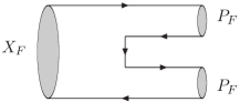
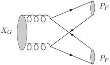
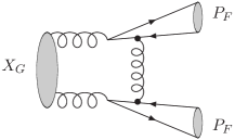
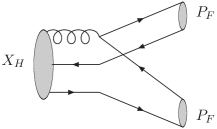
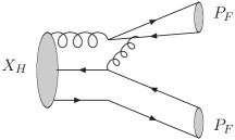
(1)	(2)	(3)	(4)	(5)
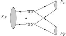
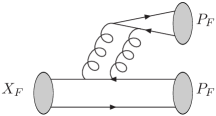
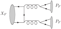
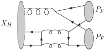
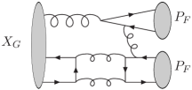
(6)	(7)	(8)	(9)	(10)

Figure 1: The diagrams corresponding, respectively, to terms in eq.(28). The last five terms are OZI suppressed ones. The processes of $X_{i}\to VV^{\prime}$ can be described by the same diagrams with the two pseudoscalar mesons in the final states replaced by two vector mesons.

The effective Hamiltonian of scalar state decaying into two pseudoscalar mesons can be written as [17]

$$\mathcal{H}^{PP}_{eff} = f_{1}\mathrm{Tr}[X_{F}P_{F}P_{F}]+f_{2}X_{G}\mathrm{Tr}[P_{F}P_{F}]+f_{3}X_{G}\mathrm{Tr}[P_{F}]\mathrm{Tr}[P_{F}]+f_{4}\mathrm{Tr}[X_{H}P_{F}P_{F}]$$ (28)

$$+ f_{5}\mathrm{Tr}[X_{H}P_{F}]\mathrm{Tr}[P_{F}]+f_{6}\mathrm{Tr}[X_{F}]\mathrm{Tr}[P_{F}P_{F}]+f_{7}\mathrm{Tr}[X_{F}P_{F}]\mathrm{Tr}[P_{F}]$$

$$+ f_{8}\mathrm{Tr}[X_{F}]\mathrm{Tr}[P_{F}]\mathrm{Tr}[P_{F}]+f_{9}\mathrm{Tr}[X_{H}]\mathrm{Tr}[P_{F}P_{F}]+f_{10}\mathrm{Tr}[X_{H}]\mathrm{Tr}[P_{F}]\mathrm{Tr}[P_{F}].$$

Here $X_{F,G,H}$ are the quarkonia, glueball and hybrid states. $X_{F,H}$ are diagonal matrices $X_{F,H}=diag(X_{F,H}^{1},X_{F,H}^{2},X_{F,H}^{3})$. In terms of the physical component, we have

$$X_{F}^{1}=X_{F}^{2}={1\over\sqrt{2}}|N\rangle=\sum_{i}{x_{i}\over\sqrt{2}}X_{i},\;\;X_{F}^{3}=|S\rangle=\sum_{i}y_{i}X_{i},$$

$$X_{H}^{1}=X_{H}^{2}={1\over\sqrt{2}}|\xi_{N}\rangle=\sum_{i}\frac{w_{i}}{\sqrt{2}}X_{i},\;\;X_{H}^{3}=|\xi_{S}\rangle=\sum_{i}v_{i}X_{i},$$

$$X_{G}=|G\rangle=\sum_{i}z_{i}X_{i}.$$ (29)

$P_{F}$ is the nonet pseudoscalar mesons,

$$P_{F}=\left(\begin{array}[]{ccc}\frac{\pi^{0}}{\sqrt{2}}+\frac{x_{\eta}\eta+x_{\eta^{\prime}}\eta^{\prime}}{\sqrt{2}}&\pi^{+}&K^{+}\\ \pi^{-}&-\frac{\pi^{0}}{\sqrt{2}}+\frac{x_{\eta}\eta+x_{\eta^{\prime}}\eta^{\prime}}{\sqrt{2}}&K^{0}\\ K^{-}&\bar{K}^{0}&y_{\eta}\eta+y_{\eta^{\prime}}\eta^{\prime}\end{array}\right).$$ (33)

In the above, $x_{\eta}=y_{\eta^{\prime}}=(\cos\theta-\sqrt{2}\sin\theta)/\sqrt{3}$, $x_{\eta^{\prime}}=-y_{\eta}=(\sin\theta+\sqrt{2}\cos\theta)/{\sqrt{3}}$ with $\theta=-19.1^{\circ}$ being the $\eta-\eta^{\prime}$ mixing angle[18].

The corresponding diagram representation for each term $f_{i}$ is shown in Figure 1. The terms $f_{6-10}$ in the above effective Hamiltonian describing the decay modes with two meson final states are OZI suppressed as can be seen from Figure 1((6)-(10)). The contributions from these terms can be neglected to a good approximation. Within this approximation, 5 parameters (actually 4 parameters $\xi_{i}=f_{1+i}/f_{1}$ when considering ratios of branching ratios) are needed to describe decay modes with two pseudoscalar mesons in the final states.

If the $X(1812)$ state is indeed the fifth member of the QGH mixing scheme, one has one more data point, the mass, to constrain the parameters. Totally we now have five eigen-masses of $f_{0}(1370)$, $f_{0}(1500)$, $f_{0}(1710)$, $f_{0}(1790)$, $X(1812)$, and nine ratios of the branching ratios listed in Table 1 to determine the 11 parameters (7 parameters in the mass matrix plus the 4 parameters $\xi_{i}$ in the decay amplitudes). One therefore is able to carry out a $\chi^{2}$ analysis with 3 degrees of freedom to test the mechanism in detail. In our fit, we also made sure that the allowed parameter space should not result in any predicted branching ratio to be larger than unity when data on total decay widths of relevant particles are used.

	Experiment data[19]	Best fit
$\frac{\Gamma(f_{0}(1370)\rightarrow\pi\pi)}{\Gamma(f_{0}(1370)\rightarrow K\bar{K})}$	$2.17\pm 0.90$	2.22
$\frac{\Gamma(f_{0}(1370)\rightarrow\eta\eta)}{\Gamma(f_{0}(1370)\rightarrow K\bar{K})}$	$0.35\pm 0.30$	0.42
$\frac{\Gamma(f_{0}(1500)\rightarrow\pi\pi)}{\Gamma(f_{0}(1500)\rightarrow\eta\eta)}$	$5.56\pm 0.93$	5.45
$\frac{\Gamma(f_{0}(1500)\rightarrow K\bar{K})}{\Gamma(f_{0}(1500)\rightarrow\pi\pi)}$	$0.33\pm 0.07$	0.32
$\frac{\Gamma(f_{0}(1500)\rightarrow\eta\eta^{\prime})}{\Gamma(f_{0}(1500)\rightarrow\eta\eta)}$	$0.53\pm 0.23$	0.26
$\frac{\Gamma(f_{0}(1710)\rightarrow\pi\pi)}{\Gamma(f_{0}(1710)\rightarrow K\bar{K})}$	$0.20\pm 0.03$	0.20
$\frac{\Gamma(f_{0}(1710)\rightarrow\eta\eta)}{\Gamma(f_{0}(1710)\rightarrow K\bar{K})}$	$0.48\pm 0.19$	0.27
$\frac{\Gamma(f_{0}(1710)\rightarrow\eta\eta^{\prime})}{\Gamma(f_{0}(1710)\rightarrow K\bar{K})}$	$<0.04(90\%\;\mathrm{C.L.})$	0.007
$\frac{\Gamma(f_{0}(1790)\rightarrow\pi\pi)}{\Gamma(f_{0}(1790)\rightarrow K\bar{K})}$	$3.88^{+5.6}_{-1.9}\cite[cite]{[\@@bibref{}{bbes}{}{}]}$	3.84
$M_{X(1812)}$(MeV)[1]	$1812^{+19}_{-26}(\mathrm{stat})\pm 18(\mathrm{syst})$	1809
$M_{f_{0}(1790)}$(MeV)[2]	$1790^{+40}_{-30}$	1797
$M_{f_{0}(1710)}$(MeV)[14]	$1714\pm 5$	1714
$M_{f_{0}(1500)}$(MeV)[14]	$1507\pm 5$	1510
$M_{f_{0}(1370)}$(MeV)[14]	$1350\pm 150$	1242

Table 1: The measured and predicted central values for branching ratios and masses. The minimal $\chi^{2}$ per degree of freedom is 1.26.

The best fit values for relevant quantities from our $\chi^{2}$ analysis are listed in Tables 1 and 2. The minimal $\chi^{2}$ per degree of freedom of our fit is 1.26 indicating a good fit. The data fitting quality has been improved compared with our previous study. The QGH mixing scheme is a reasonable scheme to describe the mixing of the five $0^{+}(0^{++})$ states. In Table 2 we also list estimates for the 68.3% error tolerance in the parameters by allowing minimal $\chi^{2}$ per degree of freedom to float up by an amount accordingly (with three degrees of freedom it is 1.17). We see that the $\chi^{2}$ is not sensitive to $\xi_{4}$. More data are need to have a better determination for these parameters.

The best fit values for the mxing matrix elements are given by

$$U=\left(\begin{array}[]{lllll}-0.971&-0.197&-0.106&-0.074&-0.031\\ -0.215&+0.967&+0.106&+0.081&+0.032\\ -0.087&-0.143&+0.403&+0.888&+0.146\\ +0.048&+0.070&-0.707&+0.429&-0.557\\ +0.020&+0.029&-0.562&+0.127&+0.817\end{array}\right).$$

We see that the dominant component of $X(1812)$ is $s\bar{s}g$, whereas the $(u\bar{u}+d\bar{d})g/\sqrt{2}$ is the dominant one in $f_{0}(1790)$. The main components of $f_{0}(1710)$, $f_{0}(1500)$ and $f_{0}(1370)$ are S, glueball(G) and N, respectively.

Parameter	Best fit and errors	Parameter	Best fit and errors
		e	$20^{+8}_{-12}$ (MeV)
$M_{\xi_{S}}$	$1807^{+58}_{-7}$ (MeV)	f	$97^{+7}_{-6}$ (MeV)
$M_{\xi_{N}}$	$1794^{+7}_{-23}$ (MeV)	$\xi_{1}$	$0.83^{+0.07}_{-0.03}$
$M_{G}$	$1465^{+9}_{-9}$ (MeV)	$\xi_{2}$	$0.53^{+0.28}_{-0.37}$
$M_{S}$	$1670^{+10}_{-11}$ (MeV)	$\xi_{3}$	$0.92^{+0.55}_{-0.73}$
$M_{N}$	$1336^{+17}_{-10}$ (MeV)	$\xi_{4}$	$-3.08^{+3.41}_{-1.65}$

Table 2: The values for the parameters in the mass matrix $M$ and the ratios $\xi_{i}=f_{1+i}/f_{1}$ ($i=1\sim 4$) in the decay effective Hamiltonian $\mathcal{H}^{PP}_{eff}$.

3 QGH Predictions for $X(1812)$ and $f_{0}(1790)$ decays

Predictions can be made for $X(1812)$ and $f_{0}(1790)$ decays using the QGH mixing scheme with parameters determined in the previous section. These predictions can be used to further test the QGH mixing mechanism and the mixing pattern suggested. We will concentrate on two pseudoscalar $PP^{\prime}$ and two vector $VV^{\prime}$ decays here.

$X(1812)(f_{0}(1790))\to PP^{\prime}$

The decay amplitudes for two-pseudoscalar-meson decays can be obtained using eq.(28). With the numerical values determined for the parameters we obtain

$$B(X(1812)\to\pi\pi):B(X(1812)\to K\bar{K}):B(X(1812)\to\eta\eta):B(X(1812)\to\eta\eta^{\prime})$$

$$=4:37:33:0.3,$$

$$B(f_{0}(1790)\to\pi\pi):B(f_{0}(1790)\to K\bar{K}):B(f_{0}(1790)\to\eta\eta):B(f_{0}(1790)\to\eta\eta^{\prime})$$

$$=17:4:10:54.$$

The above ratios also stand for $B(J/\psi\to\gamma X(1812)\to\gamma PP^{\prime})$ and $B(J/\psi\to\gamma f_{0}(1790)\to\gamma PP^{\prime})$.

The normalization of the above branching ratios can be fixed by using the measured value of $B(f_{0}(1710)\rightarrow K\bar{K})=0.38^{+0.09}_{-0.19}$ [14] and the measured widths for the $X_{i}$ states. We obtain the corresponding values for $\Gamma(X(1812)(f_{0}(1790))\to PP^{\prime})$ given in Table 3. The large branching ratios for $X(1812)\to\bar{K}K,\eta\eta$ and $f_{0}(1790)\to\eta\eta^{\prime}$ are good tests for this mechanism.

We remark that to guarantee the resultant branching ratios of $X_{i}\to PP^{\prime}$ to be less than unity (which must be) is a non-trivial task since we have used experimental data for the decay widths. The success increases our confidence on the QGH mixing scheme.

$BR(X(1812)\rightarrow\pi\pi)$	$4.4\%$
$BR(X(1812)\rightarrow K\bar{K})$	$37.1\%$
$BR(X(1812)\rightarrow\eta\eta)$	$32.6\%$
$BR(X(1812)\rightarrow\eta\eta^{\prime})$	$0.29\%$
$BR(f_{0}(1790)\rightarrow\pi\pi)$	$16.8\%$
$BR(f_{0}(1790)\rightarrow K\bar{K})$	$4.4\%$
$BR(f_{0}(1790)\rightarrow\eta\eta)$	$9.8\%$
$BR(f_{0}(1790)\rightarrow\eta\eta^{\prime})$	$54.5\%$

Table 3: The central values for the branching ratios of $X(1812)\to PP^{\prime}$ and $f_{0}(1790)\to PP^{\prime}$.

$X(1812)(f_{0}(1790))\to VV^{\prime}$

The two-vector-meson decay modes are important ones to study since in fact the resonance $X(1812)$ is observed in the $VV^{\prime}$ channel. The effective Hamiltonian is similar to that for the Pseudoscalar meson case with certain modifications. Corresponding to each of the terms for $P_{F}P_{F}$ in eq.(28), there are two terms $V^{\mu\nu}V_{\mu\nu}/2$ ($V^{\mu\nu}=\partial^{\mu}V^{\nu}-\partial^{\nu}V^{\mu}$) and $V^{\mu}V_{\mu}$. Here $V$ is the nonet vector meson states,

$$V=\left(\begin{array}[]{ccc}\frac{\rho^{0}}{\sqrt{2}}+{\omega\over\sqrt{2}}&\rho^{+}&K^{*+}\\ \rho^{-}&-\frac{\rho^{0}}{\sqrt{2}}+\frac{\omega}{\sqrt{2}}&K^{*0}\\ K^{*-}&\bar{K}^{*0}&\phi\end{array}\right).$$ (38)

We will denote the couplings by $g_{i}$ and $g_{i}a_{i}$ for the two terms respectively for $VV^{\prime}$ decays, in place of $f_{i}$ for $PP^{\prime}$ decays. For example, the terms corresponding to $f_{1}\mathrm{Tr}[X_{F}P_{F}P_{F}]$ will be written as $(1/2)g_{1}\mathrm{Tr}[X_{F}V^{\mu\nu}V_{\mu\nu}]+g_{1}a_{1}\mathrm{Tr}[X_{F}V^{\mu}V_{\mu}]$. To the leading approximation one can neglect the OZI suppressed amplitudes $g_{6-10}$. We obtain[20]

$$A(X_{i}\rightarrow\rho\rho) = \sqrt{3}\bigg{(}\tilde{g}_{1}{x_{i}}+\sqrt{2}\tilde{g}_{2}z_{i}+\tilde{g}_{4}{w_{i}}\bigg{)},$$

$$A(X_{i}\rightarrow K^{*}\bar{K^{*}}) = \bigg{(}\tilde{g}_{1}{x_{i}}+\tilde{g}_{1}\sqrt{2}y_{i}+2\sqrt{2}\tilde{g}_{2}z_{i}+\tilde{g}_{4}\sqrt{2}v_{i}+\tilde{g}_{4}{w_{i}}\bigg{)},$$

$$A(X_{i}\rightarrow\omega\omega) = \bigg{(}\tilde{g}_{1}{x_{i}}+\tilde{g}_{2}\sqrt{2}z_{i}+2\sqrt{2}\tilde{g}_{3}z_{i}+\tilde{g}_{4}{w_{i}}+{2}\tilde{g}_{5}w_{i}\bigg{)},$$

$$A(X_{i}\rightarrow\omega\phi) = \bigg{(}2\sqrt{2}\tilde{g}_{3}z_{i}+\sqrt{2}\tilde{g}_{5}v_{i}+\tilde{g}_{5}{w_{i}}\bigg{)},$$ (39)

where $\tilde{g}_{j}\approx g^{\prime}_{j}\epsilon_{{}_{V_{1}}}\cdot\epsilon_{{}_{V_{2}}}$ with $g^{\prime}_{j}=g_{j}(p_{1}\cdot p_{2}+a_{j})$. Here we have only kept S-wave contribution since the decays are all close to the threshold and the dominant contribution comes from the S-wave term. With this approximation, there is just one parameter $g^{\prime}_{j}$ to consider for each of the terms.

Unfortunately at present not much experimental information is available for $VV^{\prime}$ decays except $J/\psi\to\gamma X(1812)\to\gamma\omega\phi$. Further theoretical considerations are needed to clarify the situation and make useful predictions. To this end we notice, from eq.(2), that the physical state $X(1812)$ and $f_{0}(1790)$ are dominated by $\xi_{S}=\bar{s}sg$ and $\xi_{N}=(\bar{u}u+\bar{d}d)g/\sqrt{2}$. If the parameters $g^{\prime}_{1-5}$ are within a factor of o(1) order, one can neglect terms proportional to $x_{i}$, $y_{i}$ and $z_{i}$ in eq.(39) for $X(1812)$ and $f_{0}(1790)$ $VV^{\prime}$ decays. With this approximation the decay amplitudes depend on only two unknown parameters, $g^{\prime}_{4}$ and $g^{\prime}_{5}$. The ratios $b_{1}=\Gamma(X(1812)\to\rho\rho)/\Gamma(X(1812)\to\omega\phi)$, $b_{2}=\Gamma(X(1812)\to\omega\omega)/\Gamma(X(1812)\to\omega\phi)$, $b_{3}=\Gamma(X(1812)\to K^{*}\bar{K^{*}})/\Gamma(X(1812)\to\omega\phi)$ and $b_{4}=\Gamma(f_{0}(1790)\to\omega\omega)/\Gamma(b_{0}(1790)\to\rho\rho)$ depend on just one parameter $\beta=g^{\prime}_{5}/g^{\prime}_{4}$. In Figure 2, we show the ratios for $b_{i}$ for $\beta$ varying from 0.3 to 3 for illustration. We see that the relative branching ratios can change a large range. When more experimental data become available, information on the parameter $\beta$ will be extracted.

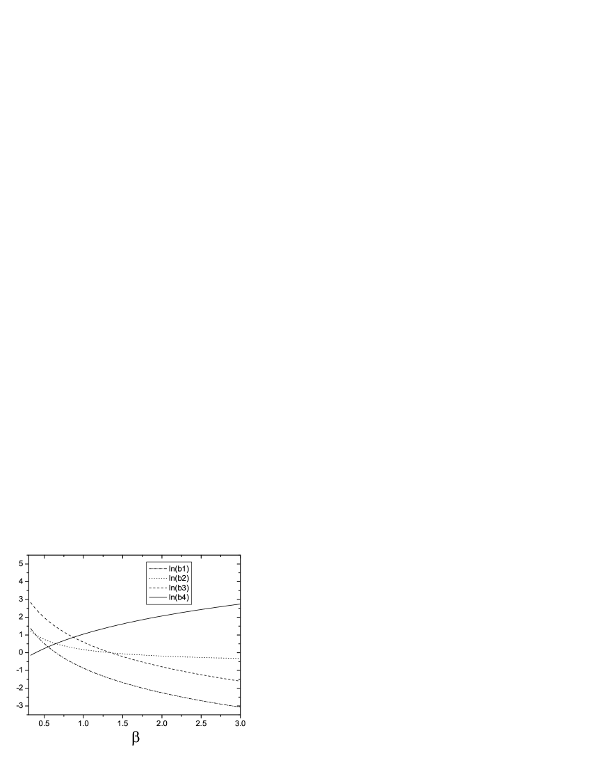
Figure 2: The dependence of $b_{i}$ on the parameter of $\beta$.

We now make an estimate of the branching ratio for $J/\psi\to\gamma X(1812)$. The transition matrix element of $J/\psi\rightarrow\gamma X_{i}$ can be written as

$$\langle\gamma X_{i}|J/\psi\rangle=x_{i}\langle\gamma N|J/\psi\rangle+y_{i}\langle\gamma S|J/\psi\rangle+z_{i}\langle\gamma G|J/\psi\rangle+w_{i}\langle\gamma\xi_{N}|J/\psi\rangle+v_{i}\langle\gamma\xi_{S}|J/\psi\rangle.$$ (40)

If the SU(3) symmetry applies, we would have

$$\langle\gamma S|J/\psi\rangle=\langle\gamma N|J/\psi\rangle/\sqrt{2}\;\;\;\mathrm{and}\;\;\;\langle\gamma\xi_{S}|J/\psi\rangle=\langle\gamma\xi_{N}|J/\psi\rangle/\sqrt{2},$$ (41)

and the relations [21, 22] roughly hold

$$\langle\gamma G|J/\psi\rangle:\langle\gamma\xi_{S}|J/\psi\rangle:\langle\gamma S|J/\psi\rangle\sim 1:\sqrt{\alpha_{s}}:\alpha_{s}.$$ (42)

We obtain an estimation

$$\Gamma(J/\psi\rightarrow\gamma X_{i})=\frac{|\mathbf{k}_{{}_{i}}|}{24\pi M_{J/\psi}^{2}}\big{[}\alpha_{s}(\sqrt{2}x_{i}+y_{i})+\sqrt{\alpha_{s}}(v_{i}+\sqrt{2}w_{i})+z_{i}\big{]}^{2}|M(J/\psi\rightarrow\gamma G)|^{2},$$ (43)

where $\mathbf{k}_{i}$ is the three-momentum of final states in the center of mass frame of $J/\psi$.

To obtain information on $|M(J/\psi\to\gamma G)|^{2}$ and therefore the branching ratios for $J/\psi\to\gamma X(1812)(f_{0}(1790))$, we use experimental data on $B(J/\psi\rightarrow\gamma f_{0}(1710)\rightarrow\gamma K\bar{K})=8.5^{+1.2}_{-0.9}\times 10^{-4}$, $B(f_{0}(1710)\rightarrow K\bar{K})=0.38^{+0.09}_{-0.19}$ [14], and obtain the ranges and central values (in the brakect) in the following with $\alpha_{s}=0.26$.

$$|M(J/\psi\to\gamma G)|^{2}=0.005\sim 0.016(0.007)\mathrm{GeV}^{2},$$

which leads to

$$B(J/\psi\rightarrow\gamma X(1812)) = (0.3\sim 1.0(0.4))\%,$$

$$B(X(1812)\rightarrow\omega\phi) = (1.8\sim 11.5(6.5))\%,$$

$$B(J/\psi\to\gamma f_{0}(1790)) = (0.3\sim 0.9(0.4))\%.$$ (44)

Obviously, the numbers obtained are based on crude approximation which should be taken as an order of magnitude estimate.

4 Discussions and Conclusions

In our earlier work[7], based on the experimental measurements on the four $0^{+}$ mesons ($f_{0}(1370),f_{0}(1500),f_{0}(1710)$ and $f_{0}(1790)$), we suggested that the basis must be enlarged to include hybrid states to have a unified description of $0^{+}$ states, the QGH mixing scheme. Because there are two independent states $(u\bar{u}+d\bar{d})g/\sqrt{2}$ and $(s\bar{s})g$ for the hybrids of isospin singlet, we predict existence of an extra $0^{+}$ meson. The new state $X(1812)$ discovered recently by the BES collaboration fits in such a picture very nicely.

Based on the ansatz for the mixing pattern of eq.(6) in the QGH scheme, we carry out a $\chi^{2}$ analysis to obtain the mixing matrix and the concerned parameters in the effective lagrangian for $0^{+}\rightarrow PP^{\prime}$ using all avaliable experimental data on the spectra and decay branching ratios of the five members. We obtain a rather satisfactory result with the minimal $\chi^{2}$ to be 3.79 for three degrees of freedom. This fit can explain the relatively large branching ratio of decay mode $X(1812)\rightarrow\phi\omega$ observed by the BES collaboration [1] which was supposed to be a double-OZI suppressed process for usual quarkonia state.

It is noticed that after fitting the measured values of spectra and branching ratios, we find that the masses of $M_{\xi_{S}}$ and $M_{\xi_{N}}$ in the mixing matrix are close, because the masses of $f_{0}(1790)$ and $X(1812)$ are not far apart. That is what the data imply. The situation for regular $q-\bar{q}$ system is different, as we obtain by fitting data $M_{S}-M_{N}\simeq 350$ MeV, although in the range of the usual SU(3) breaking effect. In Ref.[15] the masses of the scalar hybrids in terms of the bag model as 1.51-1.90 GeV for $(u\bar{u}+d\bar{d})g/\sqrt{2}$ and 2.0-2.1 GeV for $s\bar{s}g$. If considering the upper limit, the difference for hybrid states is indeed very small. The closeness may be understood that due to the gluon existence in the state, the flavor SU(3) breaking becomes milder. Of course this allegation needs to be tested in the future.

With all the information available, we have made theoretical predictions on the decay branching ratios of $f_{0}(1790)$, $X(1812)$ into two pseudoscalar mesons. We find that the main decay channel of $X(1812)$ are $K\bar{K}$ and $\eta\eta$. If these predictions are confirmed by experiment, it implies that the main content of $X(1812)$ is $s\bar{s}g$. In fact, the branching ratios of other modes are not too small and have the same order of magnitude as $B(X(1812)\to\omega\phi)$, and can be measured in the future experiments. Instead, among all the decay channels of $B(f_{0}(1790)\to K\bar{K},\;\eta\eta)$ are relatively small, but $B(f_{0}(1790)\to\eta\eta^{\prime},\;\pi\pi)$ would be large. Experimentally, the two modes $f_{0}(1790)\to\pi\pi$ and $f_{0}(1790)\to K\bar{K}$ have been observed, so we suggest our experimental colleagues to measure the channel $f_{0}(1790)\to\eta\eta^{\prime},\;\eta\eta$.

At present, very limited data about the decays of $f_{0}(1370,1500,1710,1790)$ and $X(1812)$ into two vector mesons are available, therefore we have made further approximation to estimate related decays by keeping only the main terms $g^{\prime}_{4}$ and $g^{\prime}_{5}$ in the effective lagrangian for decay amplitudes. With more data in the future, the relevant parameters can be determined better.

We have also made a rough estimate of the branching ratios of $J/\Psi\to\gamma X(1812)$ and $J/\Psi\to\gamma f_{0}(1790)$. These results can provide useful information to our experimental colleagues for carrying out further tests.

Before closing this section we would like to make some comments on another alternative scenario for $X(1812)$, the four-quark state mechanism. Four-quark state can also accommodate new $0^{+}(0^{++})$ particles[23]. An immediate question arises about this scenario is that how many ground states of $0^{+}(0^{++})$ can be formed with four light quarks and how to identify the dominant component of $X(1812)$.

The number of ground states can be easily obtained by looking at the number of isospin $I=0$ states from $\bar{q}_{i}\Gamma q_{j}\bar{q}_{k}\Gamma q_{l}$. Here $i,j,k,l$ are color indices. $\Gamma$ indicates combination of Dirac matrices with appropriate Lorentz indices. We remark that when counting the number of physical $0^{+}(0^{++})$ states, the states with the same flavor structure should be counted as one state. To find the number of $I=0$ states formed from two quarks ($3$ of SU(3)) and two anti-quarks ($\bar{3}$ of SU(3)), one can decompose $3$ and $\bar{3}$ into SU(2) isospin group to have $3=1+2$ and $\bar{3}=1+\bar{2}$ and identify the $I=0$ states. There are, naively, five possible $I=0$ states given by

$$O_{\bar{s}s\bar{s}s}=\bar{s}s\bar{s}s,\;\;O_{\bar{q}s\bar{s}q}=\bar{u}s\bar{s}u+\bar{d}s\bar{s}d,\;\;O_{\bar{s}q\bar{q}s}=\bar{s}u\bar{u}s+\bar{s}d\bar{d}s,$$

$$O_{(\bar{q}q)_{0}(\bar{q}q)_{0}}=(\bar{u}u+\bar{d}d)(\bar{u}u+\bar{d}d),\;\;O_{(\bar{q}q)_{1}(\bar{q}q)_{1}}=\bar{u}d\bar{d}u+{1\over 2}(\bar{u}u-\bar{d}d)(\bar{u}u-\bar{d}d)+\bar{d}u\bar{u}d.$$

It is clear that $O_{\bar{q}s\bar{s}q}$ is the same as $O_{\bar{s}q\bar{q}s}$ as far as flavor contents are concerned and therefore should be identified as the same which we will denote as $O_{\bar{s}s\bar{q}q}$. $O_{(\bar{q}q)_{0}(\bar{q}q)_{0}}$ is the $I=0$ state formed from two $I=0$ $\bar{q}q$ structures, and $O_{(\bar{q}q)_{1}(\bar{q}q)_{1}}$ is the $I=0$ state formed from two $I=1$ $\bar{q}q$ structures.

If kinematically allowed states are dominated by $O_{\bar{s}s\bar{s}s}$, $O_{\bar{s}s\bar{q}q}$, $O_{(\bar{q}q)_{0}(\bar{q}q)_{0}}$ and $O_{(\bar{q}q)_{1}(\bar{q}q)_{1}}$, should have their dominant decay modes to be of the types: $(\phi\phi,\;\eta^{(^{\prime})}\eta^{(^{\prime})})$, $(\phi\omega$,$\bar{K}^{*}K^{*},\;$ $\eta^{(^{\prime})}\eta^{(^{\prime})},\;\bar{K}K)$, $(\omega\omega,\;\;\eta^{(^{\prime})}\eta^{(^{\prime})})$, and $(\rho\rho,\;\pi\pi)$, respectively. The $X(1812)$ state, if dominated by a four-quark state, should have large $O_{\bar{s}s\bar{q}q}$ component.

The above discussion shows that if the $X(1812)$ is a $0^{+}$ composed of four quarks, there should be another three $0^{+}$ states. If these states mix with quarkonia and glueball, then there should be seven $0^{+}$ states. Interesting enough, these can accommodate $f_{0}(600)$, $f_{0}(980)$, $f_{0}(1370)$, $f_{0}(1500)$, $f_{0}(1710)$, $f_{0}(1790)$ and $X(1812)$. This is different than the QGH mixing scheme where $f_{0}(600)$ and $f_{0}(980)$ are left out in the picture which may be accounted for by introducing molecular states. The detailed mixing is difficult to study due to lack of both experimental and theoretical information. More theoretical and experimental studies are needed.

Acknowledgements: We thank Dr. S. Jin and Dr. X. Shen for useful discussions concerning the properties of the new resonant state $X(1812)$. This work is partly supported by NNSFC and NSC.

References

[1] BES Collaboration, M. Ablikim et al, arXiv: hep-ex/
0602031.
[2] BES Collaboration, M. Ablikim et al., Phys. Lett.
B607, 243(2005).
[3] F. Giacosa, Th. Gutsche, V.E. Lyubovitskij and A.
Faessler, Phys. Rev. D72, 094006 (2005); F. Giacosa, Th.
Gutsche, V.E. Lyubovitskij and A. Faessler, Phys. Lett. B622,
277-285 (2005); S. Narison, Nucl. Phys. B509, 312-356 (1998).
[4] D.M. Li, H. Yu, Q.X. Shen, Commun. Theor. Phys. 34
507-512 (2000); D.M. Li, H. Yu, Q.X. Shen, Eur. Phys. J. C19
529-533 (2001).
[5] F.E. Close and A. Kirk, Phys. Lett. B483, 345-352
(2000).
[6] C. Amsler and F.E. Close, Phys. Lett. B353,
385 (1995); C. Amsler and F.E. Close, Phys. Rev. D53, 295
(1996).
[8] D. Horn and J. Mandula, Phys. Rev. D17, 898
(1978).
[9] N. Isgur and J. Paton, Phys. Rev. D31, 2910
(1985); N. Isgur, R. Kokoski and J. Paton, Phys. Rev. Lett. 54,
869 (1985); F. E. Close and P. R. Page, Nucl. Phys. B443, 233
(1995); T. Barnes, F.E. Close and E.S. Swanson, Phys. Rev. D52, 5242 (1995); F.E. Close and S. Godfrey, Phys. Lett. B574, 210 (2003).
[10] T. Barnes and F.E. Close, Phys. Lett. B116, 365
(1982); M.S. Chanowitz and S.R. Sharpe, Phys. Lett. B132, 413
(1983); M.S. Chanowitz and S.R. Sharpe, Nucl. Phys. B222, 211
(1983).
[11] J. Govaerts et al., Nucl. Phys. B248, 1 (1984); F. de Viron and J. Govaerts, Phys. Rev. Lett. 53,2207 (1984); S.L. Zhu, Phys. Rev. D60, 014008 (1999); S.L.
Zhu, Phys. Rev. D60, 097502 (1999).
[12] C. Michael, arxiv: hep-ph/0308293; X.Q. Luo and
Y. Liu, arxiv: hep-lat/0512044; T.W. Chiu and T.H. Hsieh, arxiv:
hep-lat/0512029.
[13] S. Ishida et al., KEK Preprint 95-167, NUP-A-95-15,
November 1995, H.
[14] S. Eidelman et al., Particle Data Group, Phys. Lett. B592, 1 (2004).
[15] K.T. Chao, arxiv: hep-ph/0602190.
[16] N. Ishii, H. Suganuma and H. Matsufuru,
Proc. of. Lepton Scattering, Hadrons and QCD,
edited by A.W. Thomas et al.
(World Scientific, 2001) 252;
in Lattice 2001, Proceedings of
the XIXth International Symposium
on Lattice Filed Theory, Berlin, Germany,
edited by M. Müller-Preussker et al.
[Nucl. Phys. B (Proc. Suppl.) 106-107, 516
(2002)];
C. J. Morningstar and M. Peardon,
Phys. Rev. D60, 034509 (1999),
and references therein; J. Sexton, A.Vaccarino and D. Weingarten,
Phys. Rev. Lett. 75, 4563 (1995),
and references therein; M.J. Teper,
OUTP-98-88-P (1998), arXiv: hep-th/9812187; N. Ishii, H. Suganuma and H. Matsufuru,
Phys. Rev. D66, 014507 (2002).
[17] C.S. Gao, arXiv: hep-ph/9901367.
[18] D. Coffman et al., Phys. Rev. D38, 2695
(1988); J. Jousset et al., Phys. Rev. D41, 1389 (1990).
[19] WA102 Collaboration, D. Barberis et al., Phys. Lett.
B479, 59 (2000).
[20] V. Cirigliano, G. Ecker, H. Neufeld and A.
Pich, JHEP 0306, 012 (2003); S. Weinberg, Physica A 96,
327 (1979); J. Gasser and H. Leutwyler, Annals Phys. 158, 142
(1984); J. Gasser and H. Leutwyler, Nucl. Phys. B250, 465
(1985); G. Ecker, J. Gasser, A. Pich and E. de Rafael, Nucl. Phys.
B321, 311 (1989); G. Ecker, J. Gasser, H. Leutwyler, A. Pich
and E. de Rafael, Phys. Lett. B223, 425 (1989).
[21]F.E. Close, G. Farrar and Z.P. Li, Phys. Rev. D55, 5749 (1997).
[22]F.E. Close, An Introduction to Quarks and
Partons, Academic Press, London (1979).