PQCD analysis of exclusive $e^{+}e^{-}\to D_{[s]}^{+}D_{[s]}^{-}$ cross section at $\sqrt{s}=10.6$ GeV

Abstract

We analyze the exclusive pseudoscalar $D_{[s]}^{+}D_{[s]}^{-}$ pair production in $e^{+}e^{-}$ annihilations at $\sqrt{s}=10.6$ GeV using a non-factorized PQCD with the light-front wave function that goes beyond the peaking approximation. We compare our non-factorized analysis with the usual factorized analysis based on the peaking approximation in the calculation of the cross section for the heavy meson pair production. We also discuss the higher helicity contribution to the cross section. Our analysis provides a constraint on the size of quark transverse momentum inside the $D$ meson from the recent Belle data, $\sigma_{\rm Exp.}(e^{+}e^{-}\to D^{+}D^{-})<0.04$.

I Introduction

Recently, many theoretical works have been devoted to explain the large discrepancy between theoretical and experimental results for the charmonium production in $e^{+}e^{-}$ annihilations. For instance, the data Aubert ; Abe ; Uglov for charmonium production cross sections in $e^{+}e^{-}$ annihilations at the $B$-factory energy $\sqrt{s}=10.6$ GeV differ a lot from the theoretical predictions for both exclusive Grozin ; Bra1 ; Liu ; Liu2 ; BKL2006 and inclusive Cho processes although higher order corrections may reduce the differences Chao2006 . A couple of years ago, the Belle Collabotation Uglov reported the first measurement of the $e^{+}e^{-}\to D^{*+}D^{*-}$ and $e^{+}e^{-}\to D^{+}D^{*-}$ cross sections and polarizations at $\sqrt{s}\simeq 10.6$ GeV. They also set an upper limit on the cross section for $e^{+}e^{-}\to D^{+}D^{-}$. Interestingly, while the theoretical predictions based on the heavy quark effective theory Grozin and the constituent quark model Liu2 for $e^{+}e^{-}\to D^{*+}D^{*-}$ and $e^{+}e^{-}\to D^{+}D^{*-}$ cross sections are similar to the measured data Uglov , the predictions for $e^{+}e^{-}\to D^{+}D^{-}$ cross section are either quite smaller Grozin or somewhat larger Liu2 than the data Uglov .

The above exclusive/inclusive meson pair productions provide a unique opportunity to investigate asymptotic behaviors of various meson form factors in the framework of perturbative quantum chromodynamics(PQCD). The heavy meson pair production is of special interest since gluons carrying large momentum transfers can be rather easily accessible in the kinematic region above the threshold. Also, the wavefunctions of heavy systems may be well constrained due to the heaviness of constituents. Thus, it has been pointed out that exclusive pair production of heavy mesons can be reliably predicted within PQCD BJ .

If the factorization theorem in PQCD is applicable to exclusive processes, then the invariant amplitude for exclusive processes factorizes into the convolution of the valence quark distribution amplitude(DA) $\phi(x,q^{2})$ with the hard scattering amplitude $T_{H}$ BL . To implement the factorization theorem at high momentum transfer, the hadronic wave function plays an important role linking between long distance nonperturbative QCD and short distance PQCD. A particularly convenient and intuitive framework in applying PQCD to exclusive processes is based upon the light-front(LF) Fock-state decomposition of hadronic state. In the LF framework, the valence quark DA is computed from the valence LF wave function $\Psi_{n}(x_{i},{\bf k}_{\perp i})$ of the hadron at equal LF time $\tau=t+z/c$ which is the probability amplitude to find $n$ constituents(quarks,antiquarks, and gluons) with LF momenta $k_{i}=(x_{i},{\bf k}_{\perp i})$ in a hadron. Here, $x_{i}$ and ${\bf k}_{\perp i}$ are the LF momentum fraction and the transverse momenta of the $i$th constituent in the $n$-particle Fock-state, respectively.

To lowest order in perturbation theory of the meson form factor calculation at large momentum transfers, the hard scattering amplitude $T_{H}$ is dominated by one-gluon exchange diagrams. For the factorization theorem to be applicable in the heavy meson pair production analysis, the only consistent form of the quark DA would be the $\delta$ function, i.e. $\phi(x,q^{2})\sim\delta(x-m_{Q}/M)$ where $m_{Q}$ and $M$ are the heavy quark mass and the meson mass, respectively JP . In this so called “peaking approximation”, the momentum fraction carried out by $i$th constituent is equal to the ratio of the constituent mass to meson mass, $x_{i}=m_{i}/M$. This relation implies $M=m_{1}+m_{2}$, i.e. zero-binding energy limit.

However, as pointed out in Ref. JP , if the quark DA is not an exact $\delta$ function, i.e. ${\bf k}_{\perp}$ in the soft bound state LF wave function can play a significant role, the factorization theorem is no longer applicable. To go beyond the peaking approximation, the invariant amplitude should be expressed in terms of the LF wave function $\Psi(x_{i},{\bf k}_{\perp i})$ rather than the quark DA. In Ref. JP , the validity issue of peaking approximation for the heavy meson pair production processes was discussed using the LF model wave function $\Psi(x_{i},{\bf k}_{\perp i})\propto\exp(-M^{2}_{0}/\beta^{2})$, where $M_{0}$ is the invariant mass of the constituent quark and antiquark defined by $M^{2}_{0}=\sum_{i}({\bf k}^{2}_{\perp}+m^{2}_{i})/x_{i}$ and $\beta$ is the gaussian parameter. The limit $\beta\to 0$ corresponds to the peaking approximation(i.e. zero-binding energy limit $M=m_{1}+m_{2}$). In the analysis of the heavy-heavy system like $B_{c}(b{\bar{c}})$ meson, it was found that the effect of going beyond the peaking approximation ($\beta$ up to 100 MeV) was not important compared to the peaking approximation limit(i.e. $\beta\to 0$) JP . However, it is not yet clear if the same conclusion would apply to the heavy-light system such as $D$ and $B$ mesons. Moreover, the initial analysis limited only up to $\beta\leq 100$ MeV may not be sufficient to draw a definite conclusion on the validity of the peaking approximation.

The main purpose of this work is to extend the previous analysis JP and point out that the recent Belle data Uglov can provide a rather stringent constraint on how broad or narrow the $D^{\pm}$ meson quark DA is. Clarifying the relation between the $\beta$ value and transverse momentum, ${\bf k}_{\perp}$, is a particularly important issue since the quark DA is very sensitive to the $\beta$ value and the different shape of the quark DA could enhance or reduce the cross section for the exlcusive meson pair production in $e^{+}e^{-}$ annihilations. Incidentally, Bondar and Chernyak BC considered a rather broad quark DA(i.e. rather significant binding energy effect) instead of $\delta$-type quark DA to explain the data for the exclusive $e^{+}e^{-}\to J/\psi+\eta_{c}$ process. Ma and Si MS also previously discussed the variation of DA to explain the data for the same process.

In this work, we stress a consistency of our analysis in going beyond the peaking approximation. In particular, we confirm that the $\beta$ value in our model LF wave function is related with the transverse momentum via $\beta_{Q\bar{Q}}=\sqrt{\langle{\bf k}^{2}_{\perp}\rangle}_{Q\bar{Q}}$. As expected, the non-zero $\beta$ value corresponds to the transverse size of the meson and $\beta\to 0$ limit corresponds to the peaking approximation(i.e. zero binding energy limit) as discussed in JP . This implies that it may be significant to keep the transverse momentum ${\bf k}_{\perp}$ both in the wavefunction part and the hard scattering part together before doing any integration in the amplitude if $\beta$ is not so close to zero or the binding energy effect is not negligible. Thus, we think that the factorization of amplitude by integrating out the transverse momentum seperately in the wavefunction part and in the hard scattering part may not provide a consistent analysis to take into account the binding energy effect. This could distinguish our method from Ref.BC to take into account the binding energy effect.

We also note that our gaussian parameter $\beta$ is not chosen arbitrarily but fixed by the variational principle for the well-known linear plus Coulomb interaction motivated by QCD CJ2 , which in turn uniquely determine the shape of the quark DA in our model calculation. This implies that the recent data by the Belle collaboration Uglov provide a useful test on our model calculation.

The paper is organized as follows. In Sec. II, we describe the formulation of our light-front quark model (LFQM), which has been quite successful in describing the static and non-static properties of the low- lying mesons CJ2 ; CJ99 . In Sec. III, the transverse momentum dependent hard scattering amplitude for the meson is given within the LF framework. The contribution to the meson form factor from higher helicity components is also given in this section. In Sec.IV, the analytic continuation from spacelike region to the timelike region is introduced to obtain the cross section for the pseudoscalar meson pair($M\bar{M}$) production in $e^{+}e^{-}$ annihilations. As a validity check of our model, we also show that our result for the meson form factor obtained in Sec.III reduces to the peaking approximation in the $\beta\to 0$(i.e. zero-binding) limit. In Sec. V, we present the numerical results for the $e^{+}e^{-}\to D^{+}_{[s]}D^{-}_{[s]}$ cross section and compare with the available data. Summary and conclusions follow in Sec. VI. In the Appendix, we briefly summarize our proof of vanishing contribution from the light-front gauge part in $M=M_{0}$ limit.

II Model Description

In our LFQM, the meson wave function is given by

$$\Psi_{M}^{JJ_{z}}(x,{\bf k}_{\perp},\lambda\bar{\lambda}) = \phi(x,{\bf k}_{\perp}){\cal R}^{JJ_{z}}_{\lambda\bar{\lambda}}(x,{\bf k}_{\perp}).$$ (1)

where $\phi(x,{\bf k}_{\perp})$ is the radial wave function and ${\cal R}^{JJ_{z}}_{\lambda\bar{\lambda}}(x,{\bf k}_{\perp})$ is the spin-orbit wave function obtained by the interaction-independent Melosh transformation Melosh from the ordinary equal-time static spin-orbit wave function assigned by the quantum numbers $J^{PC}$. The meson wave function in Eq. (1) is represented by the Lorentz-invariant variables $x_{i}=p^{+}_{i}/P^{+}$, ${\bf k}_{\perp i}={\bf p}_{\perp i}-x_{i}{\bf P}_{\perp}$ and $\lambda_{i}$, where $P,p_{i}$ and $\lambda_{i}$ are the meson momentum, the momentum and the helicity of the constituent quarks, respectively.

The radial wave function $\phi(x,{\bf k}_{\perp})$ of a ground state pseudoscalar meson($J^{PC}=0^{-+}$) is given by

$$\phi(x,{\bf k}_{\perp}) = \biggl{(}\frac{1}{\pi^{3/2}\beta^{3}}\biggr{)}^{1/2}\exp(-{\vec{k}}^{2}/2\beta^{2}),$$ (2)

where the gaussian parameter $\beta$ is related with the size of the meson. Here, the longitudinal component $k_{z}$ of the three momentum is given by $k_{z}=(x_{1}-\frac{1}{2})M_{0}+(m^{2}_{2}-m^{2}_{1})/2M_{0}$ with the invariant mass

$$M^{2}_{0} = \frac{{\bf k}^{2}_{\perp}+m^{2}_{1}}{x_{1}}+\frac{{\bf k}^{2}_{\perp}+m^{2}_{2}}{x_{2}},$$ (3)

where $x_{1}=x$ and $x_{2}=1-x$. The covariant form of the spin-orbit wave function ${\cal R}^{00}_{\lambda\bar{\lambda}}(x,{\bf k}_{\perp})$ for the pseudoscalar meson is given by

$${\cal R}^{00}_{\lambda\bar{\lambda}}=-\frac{\bar{u}(p_{1},\lambda)\gamma_{5}v(p_{2},\bar{\lambda})}{\sqrt{2}[M^{2}_{0}-(m_{1}-m_{2})^{2}]^{1/2}},$$ (4)

and its explicit matrix form is given by

$${\cal R}^{00}_{\lambda\bar{\lambda}}=\frac{1}{C}\left(\begin{array}[]{cc}-k^{L}&x_{1}m_{2}+x_{2}m_{1}\\ -x_{1}m_{2}-x_{2}m_{1}&-k^{R}\end{array}\right),$$ (7)

where $C=\sqrt{2x_{1}x_{2}[M^{2}_{0}-(m_{1}-m_{2})^{2}]}$ and $k^{R(L)}=k_{x}\pm ik_{y}$. Note that $\sum_{\lambda\bar{\lambda}}R^{00\dagger}_{\lambda\bar{\lambda}}R^{00}_{\lambda\bar{\lambda}}=1$. The normalization of our wave function is given by

$$\sum_{\lambda\bar{\lambda}} \int d^{3}k|\Psi^{00}_{M}(x,{\bf k}_{\perp},\lambda\bar{\lambda})|^{2}$$ (8)

$$= \int^{1}_{0}dx\int d^{2}{\bf k}_{\perp}\biggl{(}\frac{\partial k_{z}}{\partial x}\biggr{)}|\phi(x,{\bf k}_{\perp})|^{2}=1,$$

where the Jacobian of the variable transformation $\{x,{\bf k}_{\perp}\}\to\vec{k}=({\bf k}_{\perp},k_{z})$ is given by

$$\frac{\partial k_{z}}{\partial x}=\frac{M_{0}}{4x_{1}x_{2}}\biggl{\{}1-\biggl{[}\frac{(m_{1}-m_{2})^{2}}{M^{2}_{0}}\biggr{]}^{2}\biggr{\}}.$$ (9)

The effect of the Jacobi factor has been analyzed in Ref. CJ_Jacob .

With this normalization, the root-mean-square(r.m.s.) value of the transverse momentum($\sqrt{\langle{\bf k}^{2}_{\perp}\rangle_{Q\bar{Q}}}$) is obtained via

$$\langle{\bf k}^{2}_{\perp}\rangle_{Q\bar{Q}} = e_{Q}\int d^{3}k|{\bf k}^{2}_{\perp}||\phi(x,{\bf k}_{\perp})|^{2}+(Q\leftrightarrow\bar{Q}).$$ (10)

Numerically, we confirm that $\sqrt{\langle{\bf k}^{2}_{\perp}\rangle_{Q\bar{Q}}}=\beta_{Q\bar{Q}}$. The numerical values of $\beta_{Q\bar{Q}}$ are discussed in Sec. V (see Table I).

The quark distribution amplitude(DA) of a meson, $\phi_{M,\lambda}(x,Q)$, i.e. the probability of finding collinear quarks up to the scale $Q$ in the $L_{z}=0$($s$-wave) projection of the meson wavefunction BL is defined by

$$\phi_{M,\lambda}(x,Q) = \int^{Q}[d^{2}{\bf k}_{\perp}]\Psi(x,{\bf k}_{\perp},\lambda\bar{\lambda}),$$ (11)

where $[d^{2}{\bf k}_{\perp}]=d^{2}{\bf k}_{\perp}\sqrt{\partial k_{z}/\partial x}/\sqrt{16\pi^{3}}$ for $\Psi=\Psi^{00}_{M}$.

III Hard scattering amplitude with ${\bf k}_{\perp}$-dependence

In this section, we calculate the pseudoscalar meson electromagnetic form factor in the region where the PQCD is applicable. Our calculation is carried out using the Drell-Yan-West frame DYW ($q^{+}=q^{0}+q^{3}=0$) with ${\bf q}^{2}_{\perp}=Q^{2}=-q^{2}$. The momentum assignment in the $q^{+}=0$ frame is given by

$$P = (P^{+},\frac{M^{2}}{P^{+}},{\bf 0}_{\perp}),\;P^{\prime}=(P^{+},\frac{M^{2}+{\bf q}^{2}_{\perp}}{P^{+}},{\bf q}_{\perp})$$

$$q = (0,\frac{{\bf q}^{2}_{\perp}}{P^{+}},{\bf q}_{\perp}),$$ (12)

where prime denotes the final state momentum and $q=P^{\prime}-P$ and $M$ is the physical meson mass.

As a starting point, the electromagnetic form factor of a pseudoscalar meson is given by a convolution of initial and final meson wavefunctions:

$$F^{\rm soft}_{M}(Q^{2}) = \sum_{\lambda\bar{\lambda}}\sum_{j}e_{j}\int d^{3}k\Psi^{00*}_{M}(x,{\bf k^{\prime}}_{\perp},\lambda\bar{\lambda})$$ (13)

$$\times\Psi^{00}_{M}(x,{\bf k}_{\perp},\lambda\bar{\lambda}),$$

where $d^{3}k=dxd^{2}{\bf k}_{\perp}\sqrt{\partial k_{z}/\partial x}$, ${\bf k^{\prime}}_{\perp}={\bf k}_{\perp}+x_{2}{\bf q}_{\perp}$ and $e_{j}$ is the electric charge of the struck quark.

At high momentum transfers, the meson form factor can be calculated within the leading order PQCD by means of a homogeneous Bethe-Salpeter equation for the meson wavefunction. Taking the perturbative kernel of the Bethe-Salpeter equation as a part of hard scattering amplitude $T_{H}$, one can get the meson electromagnetic form factor given by

$$F^{\rm Hard}_{M}(Q^{2}) = \int\frac{d^{3}kd^{3}l}{16\pi^{3}}\Psi^{00*}_{M}(y,{\bf l}_{\perp})T_{H}(x,y,{\bf q}_{\perp},{\bf k}_{\perp},{\bf l}_{\perp})$$ (14)

$$\times\Psi^{00}_{M}(x,{\bf k}_{\perp})$$

$$= \int\frac{d^{3}kd^{3}l}{16\pi^{3}}\phi(y,{\bf l}_{\perp}){\cal T}_{H}\phi(x,{\bf k}_{\perp}),$$

where $T_{H}$ contains all two-particle irreducible amplitudes for $\gamma^{*}+q{\bar{q}}\to q{\bar{q}}$ from the iteration of the LFQM wavefunction with the Bethe-Salpeter kernel. In the 2nd line of Eq. (14), we combined the spin-orbit wave function into the original $T_{H}$ to form a new ${\cal T}_{H}$, i.e.

$${\cal T}_{H}={\cal R}_{0}T_{H}^{(\lambda+\bar{\lambda}=0)}+{\cal R}_{\pm 1}T_{H}^{(\lambda+\bar{\lambda}=\pm 1)},$$ (15)

where

$${\cal R}_{0} = {\cal R}^{*}_{\uparrow\downarrow}(y,{\bf l}_{\perp}){\cal R}_{\uparrow\downarrow}(x,{\bf k}_{\perp})+{\cal R}^{*}_{\downarrow\uparrow}(y,{\bf l}_{\perp}){\cal R}_{\downarrow\uparrow}(x,{\bf k}_{\perp})$$

$$= 2\frac{[y_{1}m_{2}+y_{2}m_{1}][x_{1}m_{2}+x_{2}m_{1}]}{C_{0x}C_{0y}},$$

$${\cal R}_{\pm 1} = {\cal R}^{*}_{\uparrow\uparrow}(y,{\bf l}_{\perp}){\cal R}_{\uparrow\uparrow}(x,{\bf k}_{\perp})+{\cal R}^{*}_{\downarrow\downarrow}(y,{\bf l}_{\perp}){\cal R}_{\downarrow\downarrow}(x,{\bf k}_{\perp})$$ (16)

$$= 2\frac{{\bf k}_{\perp}\cdot{\bf l}_{\perp}}{C_{0x}C_{0y}},$$

with $C_{0x}=C$ and $C_{0y}=C(x\leftrightarrow y,{\bf k}\leftrightarrow{\bf l}_{\perp})$ [see below Eq. (7) for $C$]. The hard scattering amplitudes $T_{H}^{(\lambda+\bar{\lambda}=0)}$ and $T_{H}^{(\lambda+\bar{\lambda}=\pm 1)}$ in Eq. (15) represent the contributions from the ordinary-helicity and higher-helicity components, respectively.

To lowest order in perturbation theory, the hard scattering amplitude $T_{H}(x,y,{\bf k}_{\perp},{\bf l}_{\perp})$ is calculated from the time-ordered one-gluon-exchange diagrams shown in Fig. 1. The internal momenta for $(+,\perp)$-components are given by

$$k_{1} = (x_{1}P^{+}_{1},{\bf k}_{\perp}),\;k_{2}=(x_{2}P^{+}_{1},-{\bf k}_{\perp})$$

$$l_{1} = (y_{1}P^{+}_{1},y_{1}{\bf q}_{\perp}+{\bf l}_{\perp}),\;l_{2}=(y_{2}P^{+}_{1},y_{2}{\bf q}_{\perp}-{\bf l}_{\perp}).$$

Figure 1: Leading order light-front time-ordered diagrams for the meson form form factor.

In each diagram in Fig. 1, the instantaneous diagrams for the intermediate constituents are included using the technique shown in Ref. BL . In the LF gauge $A^{+}=0$, the gluon propagator is given by

$$d_{\mu\nu}=-g_{\mu\nu}+\frac{(k_{g})_{\mu}\eta_{\nu}+(k_{g})_{\nu}\eta_{\mu}}{k^{+}_{g}},$$ (18)

where $\eta^{+}=0,\eta^{-}=1$, and ${\vec{\eta}}_{\perp}=0$.

Hard scattering amplitudes for the helicity $\lambda+\bar{\lambda}$(=0 or $\pm 1$) components for the diagrams $A_{i}(i=1,2,3)$ are given by

$$T_{A_{1}}^{(\lambda+\bar{\lambda})} = \frac{\theta(y_{2}-x_{2})}{y_{2}-x_{2}}\frac{N_{A}^{(\lambda+\bar{\lambda})}+N_{A_{1}}}{D_{1}D_{2}},$$

$$T_{A_{2}}^{(\lambda+\bar{\lambda})} = \frac{\theta(x_{2}-y_{2})}{x_{2}-y_{2}}\frac{N_{A}^{(\lambda+\bar{\lambda})}+N_{A_{2}}}{D_{3}D_{4}},$$

$$T_{A_{3}}^{(\lambda+\bar{\lambda})} = \frac{\theta(x_{2}-y_{2})}{x_{2}-y_{2}}\frac{N_{A}^{(\lambda+\bar{\lambda})}+N_{A_{3}}}{D_{5}D_{6}},$$ (19)

where the energy denominators are given by

$$D_{1} = M^{2}+{\bf q}^{2}_{\perp}-\frac{({\bf k}_{\perp}+{\bf q}_{\perp})^{2}+m^{2}_{1}}{x_{1}}-\frac{{\bf k}^{2}_{\perp}+m^{2}_{2}}{x_{2}},$$

$$D_{2} = M^{2}+{\bf q}^{2}_{\perp}-\frac{(y_{1}{\bf q}_{\perp}+{\bf l}_{\perp})^{2}+m^{2}_{1}}{y_{1}}-\frac{{\bf k}^{2}_{\perp}+m^{2}_{2}}{x_{2}}$$

$$-\frac{(y_{2}{\bf q}_{\perp}+{\bf k}_{\perp}-{\bf l}_{\perp})^{2}}{y_{2}-x_{2}},$$

$$D_{3} = D_{1},$$

$$D_{4} = M^{2}+{\bf q}^{2}_{\perp}-\frac{({\bf k}_{\perp}+{\bf q}_{\perp})^{2}+m^{2}_{1}}{x_{1}}$$

$$-\frac{(y_{2}{\bf q}_{\perp}+{\bf k}_{\perp}-{\bf l}_{\perp})^{2}}{x_{2}-y_{2}}-\frac{(y_{2}{\bf q}_{\perp}-{\bf l}_{\perp})^{2}+m^{2}_{2}}{y_{2}},$$

$$D_{5} = M^{2}-\frac{{\bf k}_{\perp}^{2}+m^{2}_{1}}{x_{1}}-\frac{(y_{2}{\bf q}_{\perp}+{\bf k}_{\perp}-{\bf l}_{\perp})^{2}}{x_{2}-y_{2}}$$

$$-\frac{(y_{2}{\bf q}_{\perp}-{\bf l}_{\perp})^{2}+m^{2}_{2}}{y_{2}},$$

$$D_{6} = D_{4}.$$ (20)

The common $N_{A}$ in Eq. (III) is obtained from the Feynman gauge($g^{\mu\nu}$) part and given by

$$N_{A}^{(0)} = \frac{8}{x_{1}x_{2}y_{1}y_{2}}\biggl{[}x^{2}_{2}y_{1}y_{2}{\bf q}^{2}_{\perp}+x_{1}x_{2}{\bf l}^{2}_{\perp}+y_{1}y_{2}{\bf k}^{2}_{\perp}$$

$$+x_{2}(x_{1}y_{1}+x_{2}y_{2}){\bf l}_{\perp}\cdot{\bf q}_{\perp}+2x_{2}y_{1}y_{2}{\bf k}_{\perp}\cdot{\bf q}_{\perp}$$

$$+(x_{1}y_{1}+x_{2}y_{2}){\bf k}_{\perp}\cdot{\bf l}_{\perp}+x_{1}y_{1}m^{2}_{2}+x_{2}y_{2}m^{2}_{1}$$

$$+m_{1}m_{2}(y_{1}-x_{1})(y_{2}-x_{2})\biggr{]},$$

$$N_{A}^{(\pm 1)} = \frac{8[{\bf k}_{\perp}\cdot{\bf l}_{\perp}+x_{2}{\bf l}_{\perp}\cdot{\bf q}_{\perp}+x_{2}y_{2}m^{2}_{1}+x_{1}y_{1}m^{2}_{2}]}{x_{1}x_{2}y_{1}y_{2}},$$

where the last mass term $m_{1}m_{2}(y_{1}-x_{1})(y_{2}-x_{2})$ in $N_{A}^{(\lambda+\bar{\lambda}=0)}$ comes from the helicity flip contribution. In Eq. (III), $N_{A_{i}}(i=1,2,3)$ are obtained from the LF gauge parts proportional to $1/k^{+}_{g}$ and given by

$$N_{A_{1}} = \frac{-8}{y_{2}-x_{2}}(D_{2}+D_{4}),$$

$$N_{A_{2}} = \frac{-8}{x_{2}-y_{2}}(D_{2}+D_{4}),$$

$$N_{A_{3}} = \frac{-8}{x_{2}-y_{2}}(D_{2}-D_{4}).$$ (22)

Hard scattering amplitudes for the helicity $\lambda+\bar{\lambda}$(=0 or $\pm 1$) components for the diagrams $B_{i}(i=1,2,3)$ are given by

$$T_{B_{1}}^{(\lambda+\bar{\lambda})} = T_{A_{2}}^{(\lambda+\bar{\lambda})}(x\leftrightarrow y,{\bf k}_{\perp}\leftrightarrow-{\bf l}_{\perp}),$$

$$T_{B_{2}}^{(\lambda+\bar{\lambda})} = T_{A_{1}}^{(\lambda+\bar{\lambda})}(x\leftrightarrow y,{\bf k}_{\perp}\leftrightarrow-{\bf l}_{\perp}),$$

$$T_{B_{3}}^{(\lambda+\bar{\lambda})} = T_{A_{3}}^{(\lambda+\bar{\lambda})}(x\leftrightarrow y,{\bf k}_{\perp}\leftrightarrow-{\bf l}_{\perp}).$$ (23)

If one includes the higher twist effects such as intrinsic transverse momenta and the quark masses, the LF gauge part proportional to $1/k^{+}_{g}$ leads to a singularity although the Feynman gauge part $g_{\mu\nu}$ gives the regular amplitude. This is due to the gauge-invariant structure of the amplitudes. The covariant derivative $D_{\mu}=\partial_{\mu}+igA_{\mu}$ makes both the intrinsic transverse momenta, ${\bf k}_{\perp}$ and ${\bf l}_{\perp}$, and the transverse gauge degree of freedom $g{\bf A}_{\perp}$ be of the same order, indicating the need of the higher Fock state contributions to ensure the gauge invariance. However, we can show that the sum of six diagrams for the LF gauge part($1/k^{+}_{g}$ terms) vanishes in the limit that the LF energy differences $\Delta_{x}$ and $\Delta_{y}$ go to zero, where $\Delta_{x}$ and $\Delta_{y}$ are given by

$$\Delta_{x} = M^{2}-\frac{{\bf k}^{2}_{\perp}+m^{2}_{1}}{x_{1}}-\frac{{\bf k}^{2}_{\perp}+m^{2}_{2}}{x_{2}}=M^{2}-M^{2}_{0x}$$

$$\Delta_{y} = M^{2}-\frac{{\bf l}^{2}_{\perp}+m^{2}_{1}}{y_{1}}-\frac{{\bf l}^{2}_{\perp}+m^{2}_{2}}{y_{2}}=M^{2}-M^{2}_{0y}.$$ (24)

In the Appendix, we briefly summarize the proof.

In this work, we calculate the higher twist effects in the limit of $\Delta_{x}=\Delta_{y}=0$ to avoid the involvement of the higher Fock state contributions. Our limit $\Delta_{x}=\Delta_{y}=0$(but $\sqrt{\langle{\bf k}^{2}_{\perp}\rangle}=\beta\neq 0$) may be considered as a zeroth order approximation in the expansion of a scattering amplitude. That is, the scattering amplitude $T_{H}$ may be expanded in terms of LF energy difference $\Delta$ as $T_{H}=[T_{H}]^{(0)}+\Delta[T_{H}]^{(1)}+\Delta^{2}[T_{H}]^{(2)}+\cdots$, where $[T_{H}]^{(0)}$ corresponds to the amplitude in the zeroth order of $\Delta$. This approximation should be distinguished from the zero-binding(or peaking) approximation that corresponds to $M=m_{1}+m_{2}$ and ${\bf k}_{\perp}=\beta=0$. The point of this distinction is to note that $[T_{H}]^{(0)}$ includes the binding energy effect(i.e. ${\bf k}_{\perp},{\bf l}_{\perp}\neq 0$) that was neglected in the peaking approximation.

In zeroth order of $\Delta_{x}$ and $\Delta_{y}$, the net contribution from the LF gauge part($1/k^{+}_{g}$ terms) vanishes[see Appendix] and we only need to compute the Feynman gauge($g^{\mu\nu}$) part, i.e. $N_{A}$ and $N_{B}$, for the PQCD analysis of meson form factor. The contribution of the Feynman gauge to the diagrams $A_{i}$ is given by

$$T^{(\lambda+{\bar{\lambda}})}_{A} = \sum_{i=1}^{3}T^{(\lambda+{\bar{\lambda}})}_{A_{i}}=N^{(\lambda+{\bar{\lambda}})}_{A}\biggl{\{}\frac{\theta(y_{2}-x_{2})}{y_{2}-x_{2}}\frac{1}{D_{1}D_{2}}+\frac{\theta(x_{2}-y_{2})}{x_{2}-y_{2}}\biggl{(}\frac{1}{D_{3}D_{4}}+\frac{1}{D_{5}D_{6}}\biggr{)}\biggr{\}}$$ (25)

$$= \frac{N^{(\lambda+{\bar{\lambda}})}_{A}}{(y_{2}-x_{2})D_{1}D_{2}}\biggl{\{}\theta(y_{2}-x_{2})+\theta(x_{2}-y_{2})(1+\frac{\Delta_{xy}}{D_{12}})(1-\frac{\Delta_{xy}}{D_{2}})^{-1}(1+\frac{\Delta_{y}}{D_{12}})^{-1}\biggr{\}},$$

where $D_{12}=D_{1}-D_{2}$ and $\Delta_{xy}=\Delta_{x}+\Delta_{y}$. In the zeroth order of $\Delta_{x}$ and $\Delta_{y}$(i.e. $\Delta_{x}=\Delta_{y}=0$), Eq. (25) reduces to

$$T^{(\lambda+{\bar{\lambda}})}_{A} = \frac{N^{(\lambda+{\bar{\lambda}})}_{A}}{(y_{2}-x_{2})D_{1}D_{2}}.$$ (26)

Similarly for the diagrams $B_{i}$, we obtain

$$T^{(\lambda+{\bar{\lambda}})}_{B} = T^{(\lambda+{\bar{\lambda}})}_{A}(x\leftrightarrow y,{\bf k}_{\perp}\leftrightarrow-{\bf l}_{\perp}).$$ (27)

The hard scattering amplitude for each helicity is summarized as follows:

$$T^{(0)}_{H} = \frac{N^{(0)}_{A}}{(y_{2}-x_{2})D_{1}D_{2}}+(x\leftrightarrow y,{\bf k}_{\perp}\leftrightarrow-{\bf l}_{\perp})$$

$$= \frac{8}{y_{1}}\frac{x_{2}y_{1}y_{2}(x_{2}{\bf q}^{2}_{\perp}+2{\bf k}_{\perp}\cdot{\bf q}_{\perp})+x_{2}(x_{1}y_{1}+x_{2}y_{2}){\bf l}_{\perp}\cdot{\bf q}_{\perp}+x_{1}y_{1}m^{2}_{2}+x_{2}y_{2}m^{2}_{1}+m_{1}m_{2}(y_{1}-x_{1})(y_{2}-x_{2})}{(x_{2}{\bf q}^{2}_{\perp}+2{\bf k}_{\perp}\cdot{\bf q}_{\perp})[x_{2}y^{2}_{2}(x_{2}{\bf q}^{2}_{\perp}+2{\bf k}_{\perp}\cdot{\bf q}_{\perp})-2x^{2}_{2}y_{2}{\bf l}_{\perp}\cdot{\bf q}_{\perp}+(y_{2}-x_{2})^{2}m^{2}_{2}]}$$

$$+(x\leftrightarrow y,{\bf k}_{\perp}\leftrightarrow-{\bf l}_{\perp}),$$

$$T^{(\pm)}_{H} = \frac{N^{(\pm)}_{A}}{(y_{2}-x_{2})D_{1}D_{2}}+(x\leftrightarrow y,{\bf k}_{\perp}\leftrightarrow-{\bf l}_{\perp})$$ (28)

$$= \frac{8}{y_{1}}\frac{x_{2}{\bf l}_{\perp}\cdot{\bf q}_{\perp}+x_{2}y_{2}m^{2}_{1}+x_{1}y_{1}m^{2}_{2}+m_{1}m_{2}(y_{1}-x_{1})(y_{2}-x_{2})}{(x_{2}{\bf q}^{2}_{\perp}+2{\bf k}_{\perp}\cdot{\bf q}_{\perp})[x_{2}y^{2}_{2}(x_{2}{\bf q}^{2}_{\perp}+2{\bf k}_{\perp}\cdot{\bf q}_{\perp})-2x^{2}_{2}y_{2}{\bf l}_{\perp}\cdot{\bf q}_{\perp}+(y_{2}-x_{2})^{2}m^{2}_{2}]}+(x\leftrightarrow y,{\bf k}_{\perp}\leftrightarrow-{\bf l}_{\perp}),$$

where we neglect the terms such as ${\bf k}^{2}_{\perp}/{\bf q}^{2}_{\perp}$, ${\bf l}^{2}_{\perp}/{\bf q}^{2}_{\perp}$, and ${\bf k}_{\perp}\cdot{\bf l}_{\perp}/{\bf q}^{2}_{\perp}$ both in the energy denominators and the numerators due to the fact that ${\bf k}^{2}_{\perp}\ll{\bf q}^{2}_{\perp}$ and ${\bf l}^{2}_{\perp}\ll{\bf q}^{2}_{\perp}$ in large momentum transfer region where PQCD is applicable HW . In the hard scattering amplitudes given by Eq.(III), the time-ordered $\theta$ function disappears via $\theta(x-y)+\theta(y-x)=1$ and there is no singularity in timelike region. We also note that the helicity flip contributions, i.e. $m_{1}m_{2}(y_{1}-x_{1})(y_{2}-x_{2})$, in the numerators and the mass terms $(y_{2}-x_{2})^{2}m^{2}_{2}$ in the denominators in Eq. (III) give negligible contributions. One can easily find that our result $T^{(0)}_{H}$ in the leading twist limit reproduces the usual leading twist PQCD result, i.e. $T^{(0)}_{H}=16/(x_{2}y_{2}Q^{2})$.

IV Timelike form factor of a heavy pseuscalar meson

We now consider the PQCD analysis of the timelike form factor for the process of $e^{+}e^{-}$ annihilations into two pesudoscalar mesons. The hard contribution to the timelike form factor for the electron-positron annihilations into two pseudoscalar mesons, i.e. $e^{+}e^{-}\to M\bar{M}$, is obtained as

$$F_{M}(q^{2})=e_{1}I(q^{2},m_{1},m_{2})+e_{2}I(q^{2},m_{2},m_{1}),$$ (29)

with the amplitude $I(q^{2},m_{1},m_{2})$ given by

$$I(q^{2},m_{1},m_{2}) = \pi C_{F}\alpha_{s}\int\frac{dxdyd^{2}{\bf k}_{\perp}d^{2}{\bf l}_{\perp}}{16\pi^{3}}\sqrt{\frac{\partial k_{z}}{\partial x}}\sqrt{\frac{\partial l_{z}}{\partial y}}$$ (30)

$$\times\phi(y,{\bf l}_{\perp}){\cal T}_{H}\phi(x,{\bf k}_{\perp}),$$

where $\alpha_{s}$ is the QCD running coupling constant and $C_{F}(=4/3)$ is the color factor. We note that all the invariant masses in ${\cal R}_{0}$ and ${\cal R}_{\pm 1}$ in the spin-orbit wave function are replaced by the physical meson mass to be self-consistent with the result for the hard scattering amplitude in zeroth order of the LF energy differences $\Delta_{x}$ and $\Delta_{y}$, i.e. $\Delta_{x},\Delta_{y}\to 0$. Again, our analysis should be clearly distinguished from the peaking approximation (zero-binding limit or $\beta\to 0$) which leads to the DA $\phi_{M}(x)$ defined by Eq. (11) as the $\delta$-type function with $x_{i}=m_{i}/M$. In our zeroth order approximation of LF energy differences, we consider $\beta\neq 0$ (i.e. the effect of the transverse size of the meson). In the next section (Sec.V), we take the $\beta$ values determined from the analysis of the mass spectroscopy using our LFQM with the variational principle for the QCD-motivated effective Hamiltonian CJ2 .

Since we neglect the ${\bf k}^{2}_{\perp},{\bf l}^{2}_{\perp}$ and ${\bf k}_{\perp}\cdot{\bf l}_{\perp}$ terms compared to large ${\bf q}^{2}_{\perp}$ as we stated below in Eq. (III), we have only ${\bf k}_{\perp}({\bf l}_{\perp})\cdot{\bf q}_{\perp}$ and ${\bf q}^{2}_{\perp}$ in both numerator and denominator terms in Eq. (III). Thus, for convenience in our numerical calculation, we change the denominator in Eq. (III) to include only even powers of ${\bf k}_{\perp}$ and ${\bf l}_{\perp}$. Then the numerators of the hard scattering amplitudes $T_{H}^{(0)}$ and $T_{H}^{(\pm)}$ in Eq. (III) include both even and odd powers of ${\bf k}_{\perp}$ and ${\bf l}_{\perp}$ via the terms $({\bf k}_{\perp}\cdot{\bf q}_{\perp})^{m}$ and $({\bf l}_{\perp}\cdot{\bf q}_{\perp})^{m}$, where $m=$integer(non-negative). After the change, the generic form of the hard scattering amplitude may be given by

$$T_{H}=\frac{N(({\bf k}_{\perp}\cdot{\bf q}_{\perp})^{m},({\bf l}_{\perp}\cdot{\bf q}_{\perp})^{m})}{D({\bf q}^{2n}_{\perp},({\bf k}_{\perp}\cdot{\bf q}_{\perp})^{2n},({\bf l}_{\perp}\cdot{\bf q}_{\perp})^{2n})},$$ (31)

where $n$ and $m$ are (non-negative) integers. In Eq. (31), we show only essential terms, ${\bf k}_{\perp}\cdot{\bf q}_{\perp}$ and ${\bf l}_{\perp}\cdot{\bf q}_{\perp}$ in the numerator to explain how to obtain the nonvanishing contributions from the ordinary and the higher helicity contributions. That is, as one can see from Eqs. (15) and (III), by combining $T^{(0)}_{H}[T^{(\pm)}_{H}]$ in Eq. (31) with the spin-orbit wave function ${{\cal R}_{0}}[{\cal R_{\pm}}]$ in Eq. (III) to get ${\cal T}_{H}$ in Eq. (15) or Eq. (30), $T^{(0)}_{H}[T^{(\pm)}_{H}]$ should have even[odd] powers of $({\bf k}_{\perp}\cdot{\bf q}_{\perp})$ and $({\bf l}_{\perp}\cdot{\bf q}_{\perp})$ in the numerator since ${{\cal R}_{0}}[{\cal R_{\pm}}]$ includes even[odd] powers of ${\bf k}_{\perp}$ and ${\bf l}_{\perp}$. As a result, we can get ${\cal T}_{H}$ in Eq. (30) as a function of even powers of ${\bf k}_{\perp}$ and ${\bf l}_{\perp}$ for both ordinary and higher helicity contributions. We then analytically continue to the timelike region by changing ${\bf q}_{\perp}$ to $i{\bf q}_{\perp}$(or ${\bf q}^{2}_{\perp}\to-q^{2}$ in this case) in the form factor.

In terms of $F_{M}(q^{2})$ given by Eq. (29), the cross section of the pseudoscalar meson pair($M\bar{M}$) production in the unpolarized $e^{+}e^{-}$ annihilations is given by

$$\frac{d\sigma}{d\Omega}(e^{+}e^{-}\to M\bar{M})=\frac{3\bar{\beta}^{3}}{32\pi}\sigma_{e^{+}e^{-}\to\mu^{+}\mu^{-}}\sin^{2}\theta|F_{M}(q^{2})|^{2},$$ (32)

where $\bar{\beta}=\sqrt{1-4M^{2}/q^{2}}$ and $\sigma_{e^{+}e^{-}\to\mu^{+}\mu^{-}}=\pi\alpha^{2}/(3E^{2}_{\rm beam})$ with $E_{\rm beam}=\sqrt{q^{2}}/2$.

In the peaking approximation, the transverse momenta of the quark and antiquark are neglected and the longitudinal momentum fractions are given by $x_{1}=y_{1}=m_{1}/M$ and $x_{2}=y_{2}=m_{2}/M$ with $M=m_{1}+m_{2}$. In this approximation, the higher helicity contribution to the hard scattering amplitude also vanishes and the ordinary helicity contribution to the hard scattering amplitude given by Eq. (III) can be rewritten as

$$[T^{(0)}_{H}]_{\rm peaking} = \frac{8}{x^{3}_{2}y_{1}y^{2}_{2}}\frac{-x^{2}_{2}y_{1}y_{2}q^{2}+x_{1}y_{1}m^{2}_{2}+x_{2}y_{2}m^{2}_{1}}{q^{4}}$$ (33)

$$\;\;+(x\leftrightarrow y)$$

$$= \frac{32M\gamma}{q^{4}}\biggl{(}\frac{M}{m_{2}}\biggr{)}^{4}\biggl{[}1-\frac{q^{2}}{4M^{2}}\frac{2m_{2}}{m_{1}}\biggr{]},$$

where $\gamma=m_{1}m_{2}/M$.

Therefore, the peaking approximation of the timelike form factor of a heavy pseudoscalar meson is given by

$$[F_{M}]_{\rm peaking}(q^{2}) \propto e_{1}\int dxdy\delta(x_{i}-m_{i}/M)[T^{(0)}_{H}]_{\rm peaking}$$ (34)

$$\times\delta(y_{i}-m_{i}/M)+(1\leftrightarrow 2)$$

$$\propto \frac{1}{q^{4}}\biggl{\{}e_{1}\biggl{(}\frac{M}{m_{2}}\biggr{)}^{4}\biggl{[}1-\frac{q^{2}}{4M^{2}}\frac{2m_{2}}{m_{1}}\biggr{]}$$

$$+e_{2}\biggl{(}\frac{M}{m_{1}}\biggr{)}^{4}\biggl{[}1-\frac{q^{2}}{4M^{2}}\frac{2m_{1}}{m_{2}}\biggr{]}\biggr{\}}.$$

This reproduces the result obtained by Brodsky and Ji BJ . The form factor zero in this approximation occurs at

$$\bar{q}^{2} = \frac{q^{2}}{4M^{2}}=\frac{\frac{m_{1}}{2m_{2}}+\biggl{(}\frac{e_{2}}{e_{1}}\biggr{)}\frac{m^{3}_{2}}{2m^{3}_{1}}}{1+\biggl{(}\frac{e_{2}}{e_{1}}\biggr{)}\frac{m^{2}_{2}}{m^{2}_{1}}}.$$ (35)

Even though $m_{1}>m_{2}$, the $e_{2}$ contribution is not negligible for the heavy-heavy pseudoscalar meson system such as $B_{c}$. The reason for this is because the timelike form factor of heavy pseudoscalar meson encounters a zero and $e_{2}$ contribution in the region near the form factor zero has non-negligible effect. However, for the heavy-light quark system such as $B$ and $D$ mesons, the light quark contribution(i.e. $e_{2}$) can be safely neglected.

V Numerical Results

Table 1: The constituent quark masses $m_{q}$[GeV] and the gaussian paramters $\beta(=\sqrt{\langle{\bf k}^{2}_{\perp}\rangle})$[GeV] for the linear potential obtained from the variational principle. $q$=$u$ and $d$.

$m_{q}$	$m_{s}$	$m_{c}$	$m_{b}$	$\beta_{q\bar{q}}$	$\beta_{s\bar{s}}$	$\beta_{q\bar{s}}$	$\beta_{q\bar{c}}$	$\beta_{s\bar{c}}$	$\beta_{c\bar{c}}$	$\beta_{q\bar{b}}$	$\beta_{s\bar{b}}$	$\beta_{b\bar{b}}$
0.22	0.45	1.8	5.2	0.3659	0.4128	0.3886	0.4679	0.5016	0.6059	0.5266	0.5712	1.1452

In our numerical calculations, we use the model parameters $(m_{Q{\bar{Q}}},\beta_{Q{\bar{Q}}})$ obtained from the meson spectroscopy with the variational principle in our LFQM CJ2 for the linear confining potential. Our model parameters are summarized in Table I. As mentioned earlier, we should note that the r.m.s value of the transverse momentum in our LFQM is equal to the gaussian $\beta$ value, i.e. $\sqrt{\langle{\bf k}^{2}_{\perp}\rangle_{Q\bar{Q}}}=\beta_{Q\bar{Q}}$.

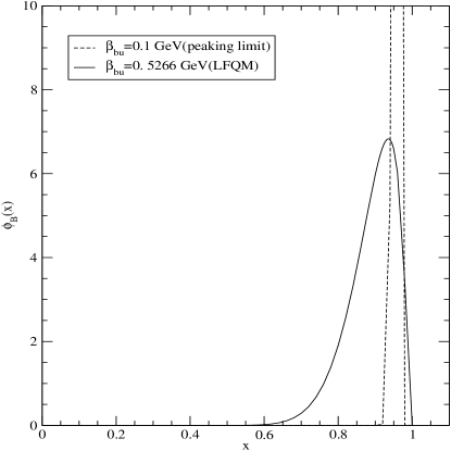
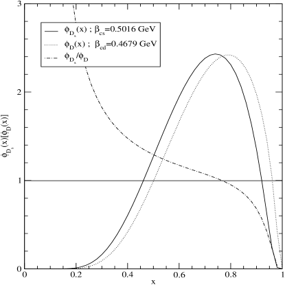
Figure 2: Normalized quark distribution amplitudes of $B$[top] and $D_{s}[D]$[bottom] mesons for different values of the gaussian parameter $\beta$.

The shape of the quark DA which depends on the $\beta$ value is important to the calculation of the cross section for the heavy meson pair production in $e^{+}e^{-}$ annihilations. We show in Fig. 2 the normalized quark DA of $B$ and $D_{s}[D]$ mesons with different values of $\beta$. For the quark DA of $B$-meson, we compare our LFQM result(solid line) with the small $\beta$ value result close to the peaking approximation, e.g. $\beta=0.1$ GeV(dashed line). As one can see, our LFQM result for the quark DA of $B$ meson shows sizable deviations from the peaking approximation. For the quark DA of $D_{s}$[solid line] and $D$[dotted line] mesons, the peak for $\phi_{D}(x)$ is located to the right of that for $\phi_{D_{s}}(x)$. This indicates that the $c$-quark carries more longitudinal momentum fraction in $D$ than in $D_{s}$ as one may expect. We also show the ratio[dash-dotted line] of $\phi_{D_{s}}(x)$ and $\phi_{D}(x)$ for the sake of comparison.

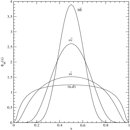
Figure 3: Normalized quark distribution amplitudes of $q\bar{q}$ with our LFQM parameters $\beta_{q\bar{q}}$.

In Fig. 3, we present also the normalized DA of various ${}^{1}S_{0}$ quarkonium($q\bar{q}$) states obtained from our LFQM parameters given in Table I. To explain the discrepancy between the NRQCD prediction Bra1 and the Belle measurement Abe for $\sigma(e^{+}e^{-}\to J/\psi+\eta_{c})$, Bondar and Chernyak(BC) BC reasoned that the discrepancy may be due to the extreme $\delta$-function-like charmonium DA adopted from NRQCD and claimed that they can fit the Belle data by choosing a rather broad DA for the charmonium state. Interestingly, our LFQM prediction for $\phi_{c\bar{c}}$ shown in Fig. 3 looks quite similar to BC’s result in a sense that the DAs for heavy quarkonium states differ from the $\delta$-function-like DA. In our model calculation, the DA gets narrower as $\beta$ gets smaller. Also the timelike form factor $F_{M}(q^{2})$ with small $\beta$ value decreases faster than that with large $\beta$ value. Since the cross section $\sigma_{e^{+}e^{-}\to M\bar{M}}$ is proportional to $|F_{M}(q^{2})|^{2}$, the cross section with small $\beta$ is small compare to that with large $\beta$. Thus, the cross section for $e^{+}e^{-}\to M\bar{M}$ can be in principle enhanced by broadening the quark DA.

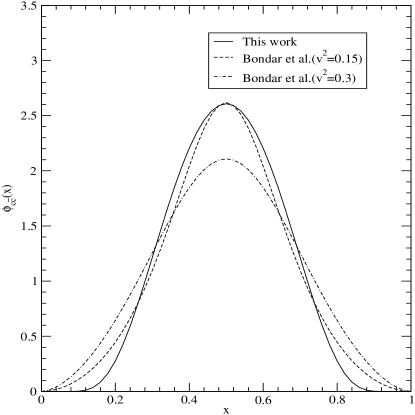
Figure 4: Normalized quark distribution amplitude of $c\bar{c}$(solid line) compare to those(dashed, dash-dotted lines) obtained from Bondar and Chernyak BC .

In Fig. 4, we compare the results of $\phi_{c\bar{c}}(x)$ in more detail. The solid and dashed(dash-dotted) lines represent our LFQM result and BC’s result BC with $v^{2}=0.15(v^{2}=0.3)$, respectively, where the parameter $v$BC represents the characteristic quark velocity in the bound state. Although there is a similarity in the quark DA between ours and BC’s results(in particular, their $v^{2}=0.15$ result), there is a rather substantial difference near the end-point region between ours and BC’s results. Since the PQCD hard scattering amplitude is typically very sensitive to the end-point values of DA, it may not be so difficult to imagine that BC’s prediction of double charm production cross sections would have made a difference depending on what $v^{2}$ value they have used. To fit the Belle measurement Abe for $\sigma(e^{+}e^{-}\to J/\psi+\eta_{c})$, they used $v^{2}=0.3$ rather than $v^{2}=0.15$. However, as we stressed earlier, the way that BCBC handled the transverse momentum effect is different from ours since they integrated out the transverse momentum seperately in the wave function part and in the hard scattering part while we didn’t factorize the hard and soft parts but integrated out the transverse momentum for the whole amplitude. We think that a consistent analysis with $\beta\neq 0$ (or non-zero binding energy) should follow our non-factorized formulation (see e.g. Eq.(30)).

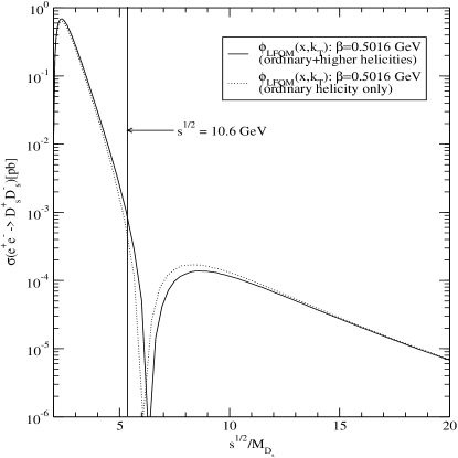
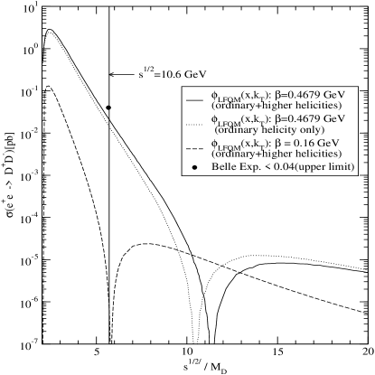
Figure 5: Cross sections for $D_{s}^{+}D_{s}^{-}$[top] and $D^{+}D^{-}$[bottom] pair productions in $e^{+}e^{-}$ annihilations with $\alpha_{s}=0.2$.

In Fig. 5, we show the cross sections for the exclusive $D_{s}^{+}D_{s}^{-}$ and $D^{+}D^{-}$ pair productions in $e^{+}e^{-}$ annihilations. The solid line represents the results including both ordinary and higher helicity contributions while the dotted line corresponds to the result of the ordinary helicity contribution only. The dashed line for $\sigma(e^{+}e^{-}\to D^{+}D^{-})$ represents the lower limit(i.e. $\beta=0.16$ GeV) for the form factor zero to occur above $\sqrt{s}=10.6$ GeV. The small black circle for $\sigma(e^{+}e^{-}\to D^{+}D^{-})$ represents the upper limit obtained from Belle Uglov , i.e. $\sigma_{\rm Exp.}(e^{+}e^{-}\to D^{+}D^{-})<0.04$. The higher helicity contribution to the cross section, i.e. the difference between solid and dotted line, is more pronounced in $e^{+}e^{-}\to D^{+}D^{-}$ than in $e^{+}e^{-}\to D_{s}^{+}D_{s}^{-}$ especially near the turnover point (or the form factor zero point). In general, the higher helicity contribution to the meson form factor increases(decreases) as quark mass decreases(increases). For instance, while the higher helicity contribution to the hard scattering amplitude is negligible in the $B$ meson form factor, it is not negligible in the pion form factor. However, the most significant in our analysis is the transverse momentum effect which delays the turnover point (see Eq. (35) for the peaking approximation). For instance, the turnover for $D_{s}[D]$ meson occurs near 6.3[11.3] by going beyond the peaking approximation while the corresponding turnover point is near $\sqrt{s}/M\sim 2.8[4.03]$ for the peaking approximation.

Numerically, we obtain the cross sections for $D_{s}^{+}D_{s}^{-}$ and $D^{+}D^{-}$ pair productions at $\sqrt{s}=10.6$ GeV with our LFQM paramters(i.e. $\beta=0.5016$ GeV for $D_{s}$ and 0.4679 GeV for $D$) as follows

$$\sigma(e^{+}e^{-}\to D_{s}^{+}D_{s}^{-}) = (8.0^{+4.4}_{-3.5})\times 10^{-4}[\rm pb],$$

$$\sigma(e^{+}e^{-}\to D^{+}D^{-}) = (0.02\pm 0.01)[\rm pb],$$ (36)

for the strong coupling constant $\alpha_{s}=0.2\pm 0.05$. Similar $\alpha_{s}$ values were used in Refs. BSJ ; KL . Our result for $\sigma(e^{+}e^{-}\to D^{+}D^{-})$ is consistent with the recent experimental data from Belle, $\sigma_{\rm Exp.}(e^{+}e^{-}\to D^{+}D^{-})<0.04$. Since $\sigma(e^{+}e^{-}\to D^{+}D^{-})$ gets larger as $\beta$ grows, the upper bound of $\sigma_{\rm Exp.}$ from Belle provides a constraint on the maximum $\beta$ value modulo the dependence on $\alpha_{s}$.

If the cross section for the $D$ meson pair production satisfies $\sigma(e^{+}e^{-}\to D^{+}D^{-})<0.04$ and its slope with respect to the momentum transfer is negative, i.e. $(d\sigma/d\sqrt{s})<0$ at $\sqrt{s}=10.6$ GeV, then we could also set the lower bound for $\beta$ value as $\beta\geq 0.16$. The shape of the $D$ meson quark DA corresponding to $\beta=0.16$ GeV is shown by dashed line in Fig. 6. If $\beta<0.16$ GeV, the $D$ meson quark DA approaches to the $\delta$-type function but $(d\sigma/d\sqrt{s})>0$ at $\sqrt{s}=10.6$ GeV due to the form factor zero occuring at $\sqrt{s}<10.6$ GeV. Due to the occurence of form factor zero for the heavy pseudoscalar meson pair production Grozin ; BJ ; BCS , more experimental data around $\sqrt{s}=10.6$ GeV are necessary to check the slope of the cross section. More data around $\sqrt{s}=10.6$ GeV would further constrain the shape of $D$ meson quark DA.

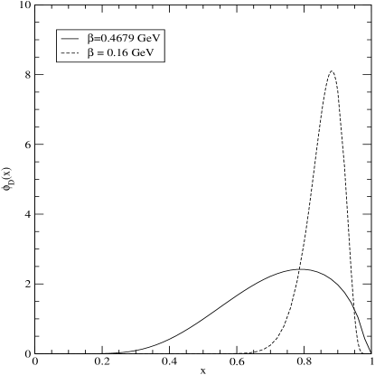
Figure 6: Lower bound for the shape of $\phi_{D}(x)$[dashed line] deduced from the assumption of $\sigma(e^{+}e^{-}\to D^{+}D^{-})<0.04$[pb] and $(d\sigma/d\sqrt{s})<0$ at $\sqrt{s}=10.6$.

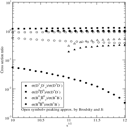
Figure 7: Our predictions[closed symbols] on the cross section ratios for various heavy pseudoscalar meson($B,B_{s},D$,and $D_{s}$) pair productions compared to the peaking approximation results[open symbols] near $\sqrt{s}=10.6$ GeV.

How about $B$ mesons? We should point out that the PQCD result of the cross section for $B^{+}B^{-}$ pair production may not be trustworthy because $\sqrt{s}=10.6$ GeV is too close to the threshold energy of $B^{+}B^{-}$ pair production. As expected, the gluon momentum transfer from the heavy quark to the light quark in $B^{+}B^{-}$ pair production at $\sqrt{s}=10.6$ GeV turns out to be only around a few hundred MeV close to the scale of $\Lambda_{QCD}$. On the other hand, the gluon momentum transfer in $D_{[s]}^{+}D_{[s]}^{-}$ pair production at $\sqrt{s}=10.6$ GeV is much larger than the scale of $\Lambda_{QCD}$. By going beyond the peaking approximation, the average gluon momentum transfer gets even larger due to the transverse momentum effect. This may justify our PQCD analysis for $D_{[s]}^{+}D_{[s]}^{-}$ pair production at $\sqrt{s}=10.6$ GeV.

Although the absolute value of the cross section for $B[B_{s}]$-meson may not be reliable near $\sqrt{s}=10.6$ GeV, it seems interesting to discuss the behavior of the ratios of cross sections such as $\sigma(e^{+}e^{-}\to B^{0}\bar{B}^{0})/\sigma(e^{+}e^{-}\to B^{+}B^{-})$ and $\sigma(e^{+}e^{-}\to B_{s}^{0}\bar{B_{s}}^{0})/\sigma(e^{+}e^{-}\to B^{+}B^{-})$. In Fig. 7, we show our predictions[closed symbols] on the cross section ratios for various heavy pseudoscalar meson($B,B_{s},D$,and $D_{s}$) pair productions in $e^{+}e^{-}$ annihilations near $\sqrt{s}=10.6$ GeV, i.e.$\sqrt{s}$ ranging from 10 to 12 GeV and compare our results with those[open symbols] obtained from the peaking approximation BJ . The open and closed diamond symbols for $\sigma(e^{+}e^{-}\to B^{0}\bar{B}^{0})/\sigma(e^{+}e^{-}\to B^{+}B^{-})$ are on top of each other and their values are almost equal to 1. In fact, the cross section ratios involving light quarks $u$ and $d$ such as $(D^{0},D)$ and $(B^{0},B)$ cases are close to 1. This is due to the negligible contribution from the diagrams where the photon is attached to the light quarks. As the replacement of light quarks by the strange quark makes those diagrams non-negligible, the cross section ratios for the cases of $(D_{s},D)$ and $(B_{s},B)$ deviate from 1 appreciably. However, most significant is again the transverse momentum effect which is pronounced in the case of $D[D_{s}]$ meson pair productions compared to $B[B_{s}]$ meson pair productions. In particular, the deviation between the open and closed symbols for the case $(D_{s},D)$ is quite dramatic compared to the case of $(B_{s},B)$.

VI Summary and Conclusion

We investigated the transverse momentum effect on the exclusive heavy meson pair productions in $e^{+}e^{-}$ annihilations within the framework of LF PQCD. The gaussian parameter $\beta$ in our model wave function is found to be related to the transverse momentum via $\beta_{Q\bar{Q}}=\sqrt{\langle{\bf k}^{2}_{\perp}\rangle_{Q\bar{Q}}}$. This relation naturally explains the zero-binding energy limit for the zero transverse momentum, i.e. $\langle M^{2}_{0}\rangle=(m_{1}+m_{2})^{2}$ and $x_{i}=m_{i}/M$ for $\beta=0$.

However, the heavy quark DA is sensitive to the value of $\beta$ and indeed substantially broad and quite different from the $\delta$-type DA according to our LFQM based on the variational principle for the QCD-motivated Hamiltonian CJ2 ; CJ99 . If the quark DA is not an exact $\delta$ function, i.e. ${\bf k}_{\perp}$ in the soft bound state LF wave function can play a significant role, the factorization theorem is no longer applicable. To go beyond the peaking approximation, the invariant amplitude should be expressed in terms of the LF wave function $\Psi(x_{i},{\bf k}_{\perp i})$ rather than the quark DA.

In going beyond the peaking approximation, we stressed a consistency by keeping the transverse momentum ${\bf k}_{\perp}$ both in the wavefunction part and the hard scattering part together before doing any integration in the amplitude. Such non-factorized analysis should be distinguished from the factorized analysis where the transverse momenta are seperately integrated out in the wavefunction part and in the hard scattering part. Even if the used LF wavefunctions lead to the similar shapes of DAs, predictions for the cross sections of heavy meson productions would apparently be different between the factorized and non-factorized analyses.

In this work, we compared our non-factorized analysis with the usual factorized analysis based on the peaking approximation and found a substantial difference between the two in the calculation of the cross section for the heavy meson pair production. We also discussed the higher helicity contribution to the cross section. Our analysis provided a constraint on the size of quark transverse momentum inside the $D$ meson from the recent Belle data, $\sigma_{\rm Exp.}(e^{+}e^{-}\to D^{+}D^{-})<0.04$. More experimental data around $\sqrt{s}=10.6$ GeV would further constrain the shape of $D$ meson quark DA and test our LFQM prediction. Application of our non-factorized PQCD analysis to the $alpha_{s}$ higher order corrections, e.g. in double charm production, would deserve further investigation.

Appendix A Proof of vanishing light-front gauge part in $M=M_{0}$ limit

The contribution of the LF gauge part($1/k^{+}_{g}$ term) to the hard scattering amplitude for diagrams $A=\sum_{i=1}^{3}A_{i}$ obtained from Eqs. (III) and (III) is given by

$$T^{(1/k^{+}_{g})}_{A} = \frac{\theta(y_{2}-x_{2})}{y_{2}-x_{2}}\frac{N_{A_{1}}}{D_{1}D_{2}}+\frac{\theta(x_{2}-y_{2})}{x_{2}-y_{2}}\biggl{(}\frac{N_{A_{2}}}{D_{3}D_{4}}+\frac{N_{A_{3}}}{D_{5}D_{6}}\biggr{)}$$ (37)

$$= -\frac{8}{(y_{2}-x_{2})^{2}}\frac{D_{2}+D_{4}}{D_{1}D_{2}}\biggl{\{}\theta(y_{2}-x_{2})+\theta(x_{2}-y_{2})\biggl{[}1+\frac{D_{2}-D_{4}}{D_{4}}\frac{D_{1}D_{2}+D_{5}(D_{2}+D_{4})}{(D_{2}+D_{4})D_{5}}\biggr{]}\biggr{\}}.$$

In terms of the LF energy differences, the relevant energy denominators can be rewritten as

$$D_{1} = \Delta_{x}-\frac{1}{x_{1}}(x_{2}{\bf q}^{2}_{\perp}+2{\bf k}_{\perp}\cdot{\bf q}_{\perp})$$

$$D_{2}+D_{4} = D_{1}+\Delta_{y}$$

$$D_{2}+D_{5} = \Delta_{x}+\Delta_{y}.$$ (38)

Eq. (37) and the corresponding LF gauge part to the diagrams $B_{i}$ lead to singularties. Fortunately, however, in the zeroth order of $\Delta_{x}$ and $\Delta_{y}$, i.e. $\Delta_{x},\Delta_{y}\to 0$ limit, one can see that the energy denominator term in $\theta(x_{2}-y_{2})$ in Eq. (37) vanishes, which leads to $\theta(y_{2}-x_{2})+\theta(x_{2}-y_{2})=1$. Thus, the LF gauge part contribution to the diagrams $A=\sum_{i=1}^{3}A_{i}$ becomes

$$T^{(1/k^{+}_{g})}_{A} = -\frac{8}{(y_{2}-x_{2})^{2}}\frac{1}{D_{2}},$$ (39)

and similarly we obtain

$$T^{(1/k^{+}_{g})}_{B} = -\frac{8}{(y_{2}-x_{2})^{2}}\frac{1}{D_{9}},$$ (40)

for the diagrams $B=\sum_{i=1}^{3}B_{i}$ . Finally, from the relation $D_{2}+D_{9}=\Delta_{x}+\Delta_{y}$, one can see that the net contribution from the LF gauge parts, i.e., $T^{(1/k^{+}_{g})}_{A}+T^{(1/k^{+}_{g})}_{B}$, vanishes exactly in the limit of $\Delta_{x}=\Delta_{y}=0$.

References

• (1) BarBar Collaboration, B. Aubert et al., Phys. Rev. Lett. 87, 162002 (2001).
• (2) Belle Collaboration, K. Abe et al., Phys. Rev. Lett. 88, 052001 (2002); Phys. Rev. Lett. 89, 142001 (2002).
• (3) Belle Collaboration, T. Uglov et al., Phys. Rev. D 70, 071101 (2004).
• (4) A. G. Grozin and M. Neubert, Phys. Rev. D 55, 272 (1997).
• (5) E. Braaten and Jungil Lee, Phys. Rev. D 67, 054007 (2003).
• (6) K. Y. Liu, Z.G. He and K. T. Chao, Phys. Lett. B 557, 45 (2003); K. Hagiwara, E. Kou and C. F. Qiao, Phys. Lett. B 570, 39 (2003).
• (7) K. Y. Liu, Z. G. He, Y. J. Zhang, and K. T. Chao, hep-ph/0311364.
• (8) G. T. Bodwin, D. Kang and J. Lee, hep-ph/0603185.
• (9) P. Cho and K. Leibovich, Phys. Rev. D 54, 6990 (1996); F. Yuan, C. F. Qiao, and K. T. Chao, Phys. Rev. D 56, 321 (1997); S. Baek, P. Ko, J. Lee, and H. S. Song, J. Korean Phys. Soc. 33, 97 (1998).
• (10) Y.-J. Zhang, Y.-J. Gao and K.-T.Chao, Phys. Rev. Lett. 96, 092001 (2006).
• (11) S. J. Brodsky and C.-R. Ji, Phys. Rev. Lett. 55, 2257 (1985).
• (12) G. P. Lepage and S. J. Brodsky, Phys. Rev. D 22, 2157 (1980).
• (13) C.-R. Ji and A. Pang, Phys. Rev. D 55, 1253 (1997).
• (14) A. E. Bondar and V. L. Chernyak, Phys. Lett. B 612, 215 (2005).
• (15) J. P. Ma and Z. G. Si, Phys. Rev. D 70, 074007 (2004).
• (16) H.-M. Choi and C.-R. Ji, Phys. Lett. B 460, 461 (1999).
• (17) H.-M. Choi and C.-R. Ji, Phys. Rev. D 59, 074015 (1999).
• (18) H. J. Melosh, Phys. Rev. D 9, 1095 (1974).
• (19) H.-M. Choi and C.-R. Ji, Phys. Rev. D 56, 6010 (1997).
• (20) S. D. Drell and T. M. Yan, Phys. Rev. Lett. 24, 181 (1970); G. West, ibid.24, 1206 (1970).
• (21) G.P. Lepage, S. J. Brodsky, T. Huang, and P. B. Mackenzie, in Particles and Fields, Proceeding of the Banff Summer Institute on Particle Physics, Banff, Alberta, Canada, 1982, edited by A. Z. Capri and A. N. Kamal(Plenum, New York, 1983), p. 143.
• (22) T. Huang, X.-G. Wu, and X.-H. Wu, Phys. Rev. D 70, 053007 (2004).
• (23) S.J. Brodsky, A.S. Goldhaber, and J. Lee, Phys. Rev. Lett. 91, 112001 (2003).
• (24) D.Kang et al., Phys. Rev. D 71, 071501(R) (2005).
• (25) M.S.Baek, S.Y.Choi, and H.S.Song, Phys. Rev. D 50, 4363 (1994).