Gravitinos from Heavy Scalar Decay

Abstract

Cosmological issues of the gravitino production by the decay of a heavy scalar field $X$ are examined, assuming that the damped coherent oscillation of the scalar once dominates the energy of the universe. The coupling of the scalar field to a gravitino pair is estimated both in spontaneous and explicit supersymmetry breaking scenarios, with the result that it is proportional to the vacuum expectation value of the scalar field in general. Cosmological constraints depend on whether the gravitino is stable or not, and we study each case separately. For the unstable gravitino with $M_{3/2}\sim$ 100GeV–10TeV, we obtain not only the upper bound, but also the lower bound on the reheating temperature after the $X$ decay, in order to retain the success of the big-bang nucleosynthesis. It is also shown that it severely constrains the decay rate into the gravitino pair. For the stable gravitino, similar but less stringent bounds are obtained to escape the overclosure by the gravitinos produced at the $X$ decay. The requirement that the free-streaming effect of such gravitinos should not suppress the cosmic structures at small scales eliminates some regions in the parameter space, but still leaves a new window of the gravitino warm dark matter. Implications of these results to inflation models are discussed. In particular, it is shown that modular inflation will face serious cosmological difficulty when the gravitino is unstable, whereas it can escape the constraints for the stable gravitino. A similar argument offers a solution to the cosmological moduli problem, in which the moduli is relatively heavy while the gravitino is light.

I Introduction

It is quite plausible that the universe once experienced the epoch where its energy density is dominated by the coherent oscillation of a scalar field. A typical example is the inflaton oscillation after the exit of the de Sitter expansion period in the slow roll inflation Linde:1981mu . Another example is dilaton and moduli fields in superstring theories.

The oscillating field eventually decays, followed by the reheating of the universe. Then, the radiation dominated era (the hot big-bang universe) commences. At the same time, however, the decay of the oscillating field may produce unwanted particles. Recently, it has been recognized that the gravitino production at the decay of a modulus field can cause cosmological disasters Endo:2006zj ; Nakamura:2006uc . It turns out that the decay width into the gravitino pair is non-suppressed and is comparable to that into other particles which couple to the moduli field with Planck suppressed interaction. Thus, the branching ratio of the moduli decay into the gravitino pair is sizable: in fact it is typically at a percentage level, or even higher. If the damped coherent oscillation of the modulus field once dominates the energy density of the universe, the overproduction of the gravitinos at its decay would cause serious problems to cosmology. The gravitino decay, if it is unstable, would spoil the success of the big-bang nucleosynthesis (BBN). In addition, these unstable gravitinos decay into the lighter superparticles, resulting in the overabundance of the lightest superparticles (LSPs). These arguments push up the gravitino mass to a region disfavored from the naturalness problem associated with the weak scale Nakamura:2006uc .

One should be aware that the problem of the gravitino overproduction may apply to other heavy scalar fields. In particular, the case of inflaton is important. After the epoch of de Sitter expansion driven by the vacuum energy, the inflaton field falls down to its true minimum and starts the damped coherent oscillation around the true minimum. Eventually it decays to reheat the universe. In many inflation models, the mass of the inflaton, or more precisely the mass of the oscillating field after the slow-roll inflation, is much larger than the weak scale. Thus, in the low energy supersymmetry, the decay into a gravitino pair is likely to be kinematically allowed. If the branching ratio is not negligible, then the gravitino production at the inflaton decay will cause serious cosmological problems.

In this paper, we would like to investigate the decay of a heavy scalar field into a gravitino pair in a general ground and consider its cosmological implications. In Sec. II, we shall first discuss the partial decay rate of the scalar decay into the gravitino pair. The decay amplitude is proportional to the vacuum expectation value (VEV) of the $F$ auxiliary component of the scalar field. We will estimate the VEV of the $F$ and thus the decay width into the gravitino pair in a very general setting. Then, in Sec. III, we will discuss cosmological problems caused by the gravitino problem. We will carry out the study in both unstable and stable gravitino cases, and identify the region of the parameter space which survives various cosmological constraints. A particular attention is paid to the case where the scalar field shares the properties with the moduli fields. We will show that the case faces a serious cosmological difficulty when the gravitino is unstable, but can survive the constraints for a light and stable gravitino. We will also point out a new window of the gravitino warm dark matter with the mass range of 10 MeV to 1 GeV. In Sec. IV, we will draw our conclusions and also discuss implications of our results to the inflation model building. In Appendix, we will explain the details on the estimation of the abundance for the long-lived superparticles.

While preparing the paper, we received a preprint Kawasaki:2006gs , which dealt with a similar subject. Our results agree with Ref. Kawasaki:2006gs , where overlap.

II Heavy scalar decay into gravitinos

Let us begin by discussing the decay of a heavy scalar field $X$ into a pair of gravitinos. To avoid unnecessary complication, we consider the case where the mass of $X$ is much heavier than the gravitino mass, $M_{X}\gg M_{3/2}$. Also we assume that $X$ is a singlet under the standard model gauge group. These assumptions are relevant for later use.

The scalar field $X$ may decay into a pair of gravitinos:

$$X\to\psi_{3/2}+\psi_{3/2}\,,$$ (1)

The decay is induced through the interaction in the supergravity. As recently calculated in Refs. Endo:2006zj ; Nakamura:2006uc , its partial decay width is given by

$$\Gamma_{3/2}=\frac{d_{3/2}^{2}}{288\pi}\frac{M_{X}^{3}}{M_{P}^{2}}\,,$$ (2)

where $M_{P}\simeq 2.4\times 10^{18}$ GeV is the reduced Planck scale. The coupling constant $d_{3/2}$ is defined by the relation

$$d_{3/2}\frac{M_{3/2}^{2}}{M_{X}}=\left\langle\left(G_{X\overline{X}}\right)^{-\frac{1}{2}}e^{G/2}G_{X}\right\rangle\,,$$ (3)

where $G$ is the total Kähler potential, $G\equiv K+\ln|W|^{2}$, with $K$ and $W$ being the Kähler potential and the superpotential, respectively. The subscript $X$ ($\overline{X}$) denotes differentiation with respect to the $X$ ($\overline{X}$) field and $\langle\cdots\rangle$ stands for the VEV. Note that the right-handed side of the above equation is the (canonically normalized) $F$-auxiliary component of the $X$ field. Therefore, $d_{3/2}$ parameterizes the supersymmetry breaking felt by the $X$ field. The parameter $d_{3/2}$ is expected to be order unity for a moduli field. If this is the case, the decay into the gravitino pair can be significant, in particular when the decays into other particles are also mediated by Planck suppressed interactions. Then, gravitinos produced at the scalar decay would lead to cosmological disasters. A more general case with less gravitino production will be discussed later.

To proceed, we now present a general expression for the VEV of the $X$’s auxiliary field. In the absence of $D$-terms, the scalar potential of the ${\cal N}=1$ supergravity is given

$$V_{\rm SUGRA}=e^{G}\left(G_{i}G^{i\bar{j}}G_{\bar{j}}-3\right),$$ (4)

where the subscript $i$ ($\bar{i}$) represents the derivative with respect to a scalar field $\phi^{i}$ ($\overline{\phi}^{\bar{i}}$) and $G^{i\bar{j}}$ is the inverse of the Kähler metric. The first derivative of the potential is obtained as

$$\frac{\partial}{\partial\phi^{i}}V_{\rm SUGRA}$$ (5)

$$= G_{i}V_{\rm SUGRA}$$

$$+e^{G}\left(G_{ij}G^{j\bar{k}}G_{\bar{k}}+G_{j}G^{j\bar{k}}{}_{i}G_{\bar{k}}+G_{j}G^{j\bar{k}}G_{\bar{k}i}\right)$$

$$= G_{i}V_{\rm SUGRA}$$

$$+e^{G}\left(G_{ij}G^{j\bar{k}}G_{\bar{k}}-G_{j}G^{j\bar{l}}G_{\bar{l}mi}G^{m\bar{k}}G_{\bar{k}}+G_{i}\right).$$

Noticing that the $F$ auxiliary field is expressed, in terms of $G$ and its derivatives, as

$$F^{i}=-G^{i\bar{j}}e^{G/2}G_{\bar{j}},$$ (6)

we find

$$\frac{\partial}{\partial\phi^{i}}V_{\rm SUGRA} = -e^{G/2}G_{ij}F^{j}-e^{G/2}(1+\tilde{V})G_{i\bar{j}}\overline{F}^{\bar{j}}$$ (7)

$$-G_{ij\bar{k}}F^{j}\overline{F}^{\bar{k}}\,,$$

with $\widetilde{V}\equiv G_{i}G^{i\bar{j}}G_{\bar{j}}-3$.

Consider first the case where the supersymmetry is spontaneously broken within the framework of supergravity. In this case, in addition to the $X$ field, we need another field $Z$ which dominantly breaks supersymmetry. At the vacuum, the VEV of the Kähler metric can be canonically normalized as $\langle G_{i\bar{j}}\rangle=\delta_{i\bar{j}}$. With this basis, the stationary point condition reads

$$0 = \left\langle\frac{\partial}{\partial X}V_{\rm SUGRA}\right\rangle$$ (8)

$$= -\left\langle e^{G/2}G_{XX}\right\rangle\langle F^{X}\rangle-\left\langle e^{G/2}G_{XZ}\right\rangle\langle F^{Z}\rangle$$

$$-\left\langle e^{G/2}(1+\widetilde{V})\right\rangle\langle\overline{F}{}^{\bar{X}}\rangle-\langle G_{XZ\bar{Z}}\rangle\langle F^{Z}\rangle\langle\overline{F}{}^{\bar{Z}}\rangle$$

$$-\langle G_{XX\overline{Z}}\rangle\langle F^{X}\rangle\langle\overline{F}{}^{\overline{Z}}\rangle-\langle G_{XX\overline{X}}\rangle\langle F^{X}\rangle\langle\overline{F}{}^{\overline{X}}\rangle$$

$$-\langle G_{XZ\overline{X}}\rangle\langle F^{Z}\rangle\langle\overline{F}{}^{\overline{X}}\rangle\,.$$

Notice that

$$\langle e^{G/2}\rangle=M_{3/2}\,,~{}~{}~{}\langle F^{Z}\rangle\simeq M_{3/2}.$$ (9)

When the mass of the $X$ field is much heavier than the gravitino mass, one finds

$$\left\langle e^{G/2}G_{XX}\right\rangle = \left\langle e^{G/2}\left(K_{XX}-\frac{W_{X}^{2}}{W^{2}}+\frac{W_{XX}}{W}\right)\right\rangle$$ (10)

$$\simeq \left\langle e^{G/2}\left(K_{XX}-K_{X}^{2}+\frac{W_{XX}}{W}\right)\right\rangle$$

$$\simeq \left\langle e^{K/2}W_{XX}\right\rangle+{\cal O}(M_{3/2})$$

$$\simeq M_{X}+{\cal O}(M_{3/2})\,.$$

In the above we have used $\langle K_{X}+W_{X}/W\rangle\ll 1$.

Using Eqs. (8), (9) and (10), the VEV of the $F$-auxiliary field can be approximately expressed as

$$\langle F^{X}\rangle \simeq -\frac{1}{M_{X}}\Bigl{(}\langle G_{XZ}\rangle M_{3/2}\langle F^{Z}\rangle$$ (11)

$$~{}~{}~{}~{}~{}~{}~{}~{}~{}+\langle G_{XZ\bar{Z}}\rangle\langle F^{Z}\rangle\langle\overline{F}{}^{\bar{Z}}\rangle\Bigr{)}\,.$$

Here, evaluation of $\langle G_{XZ}\rangle$ can be done as follows:

$$\left\langle G_{XZ}\right\rangle = \left\langle K_{XZ}+\frac{W_{XZ}}{W}-\frac{W_{X}}{W}\frac{W_{Z}}{W}\right\rangle$$ (12)

$$\simeq \left\langle K_{XZ}+\frac{W_{XZ}}{W}+K_{X}\frac{W_{Z}}{W}\right\rangle\,.$$

It is natural that $K_{X}$ and $K_{XZ}$ have VEVs comparable to $\langle X\rangle$. Furthermore, $\langle W_{Z}/W\rangle={\cal O}(1)$. Assuming that $\langle W_{XZ}/W\rangle$ is negligibly small, which is the case when the $X$ field is separated from the supersymmetry breaking sector in the superpotential, we find

$$\langle G_{XZ}\rangle={\cal O}(\langle X\rangle).$$ (13)

On the other hand, we also expect that $\langle G_{XZ\bar{Z}}\rangle=\langle K_{XZ\bar{Z}}\rangle\simeq{\cal O}(\langle X\rangle)$. To summarize the evaluations given above, we conclude

$$\left|\langle F^{X}\rangle\right|\simeq\frac{M_{3/2}^{2}}{M_{X}}\left|\langle X\rangle\right|,$$ (14)

as long as there is no cancellation between the terms in the right-handed side of Eq. (11). This in turn implies

$$d_{3/2}\simeq\left|\langle X\rangle\right|\,,$$ (15)

in the Planck unit.

Next, we would like to discuss the case where the supersymmetric anti-de Sitter vacuum is uplifted to the Minkowski one by explicit SUSY breaking terms. This is indeed the case for the KKLT set-up Kachru:2003aw , where the explicit SUSY breaking is originated from an anti-D3 brane. The scalar potential of the effective theory is then written in the form

$$V=V_{\rm SUGRA}+V_{\rm breaking}\,,$$ (16)

where $V_{\rm SUGRA}$ is the scalar potential of the supergravity given in Eq. (4). $V_{\rm breaking}$ is the explicit SUSY breaking term which is of the form

$$V_{\rm breaking}=\hat{V}f(X,\overline{X})\,,$$ (17)

with some real function $f(X,\overline{X})$.

The stationary point condition of the scalar potential (16) with respect to $X$ now reads

$$\left\langle\frac{\partial V}{\partial X}\right\rangle = \hat{V}\left\langle\frac{\partial f}{\partial X}\right\rangle+\left\langle\frac{\partial}{\partial X}V_{\rm SUGRA}\right\rangle$$ (18)

$$\simeq \hat{V}\left\langle\frac{\partial f}{\partial X}\right\rangle-M_{X}\langle F^{X}\rangle$$

$$= 0.$$

It follows from the above that

$$\langle F^{X}\rangle\simeq\frac{1}{M_{X}}\hat{V}\left\langle\frac{\partial f}{\partial X}\right\rangle.$$ (19)

By imposing that the vacuum energy vanishes at the minimum, we can determine the value of $\hat{V}$: $\hat{V}=3M_{3/2}^{2}/\langle f\rangle$. Then we obtain

$$\langle F^{X}\rangle=\frac{3M_{3/2}^{2}}{M_{X}}\left\langle\frac{\partial}{\partial X}\ln f\right\rangle.$$ (20)

To proceed further, let us see a set-up of KKLT-type Kachru:2003aw . The function $f$ is likely of the form Kachru:2003sx ; Witten:1985xb

$$\ln f=-n\ln(T+\overline{T}-\overline{C}C)\,,$$ (21)

where $T$ is an over-all modulus field and $C$ represents a (matter) field, with $n$ being some constant of order unity. With this form, we obtain $\langle\partial\ln f/\partial T\rangle={\cal O}(\langle T\rangle^{-1})={\cal O}(1)$ and $\langle\partial\ln f/\partial C\rangle\simeq{\cal O}(\langle C\rangle)$, which implies $\langle\partial\ln f/\partial X\rangle\simeq{\cal O}(\langle X\rangle)$. Thus, we reproduce the same relation (14) even when supersymmetry is explicitly broken.

It is amusing to point out that the relation (14) can be understood in softly broken global SUSY. For example, let us consider the following Lagrangian:

$$\mathcal{L} = \Bigl{[}X^{\dagger}X+\left(\theta^{2}M_{1}X^{\dagger}X+\mathrm{h.c.}\right)-\theta^{2}\bar{\theta}^{2}M_{2}^{2}X^{\dagger}X\Bigr{]}_{D}$$ (22)

$$+\left[W(X)\right]_{F}+\mathrm{h.c.},$$

with $M_{1}$ and $M_{2}$ the soft SUSY breaking parameters of order $M_{3/2}$. Here $X$ denotes a chiral supermultiplet and $X^{\dagger}$ its hermitian conjugate, unlike the rest of the paper. We can eliminate the auxiliary field $F^{X}$ by using the equations of motion

$$F^{X}=-\left(\overline{W}_{\overline{X}}+M_{1}X\right).$$ (23)

The resulting scalar potential is written

$$V=\left|M_{1}\overline{X}+W_{X}\right|^{2}+M_{2}^{2}\overline{X}X.$$ (24)

The stationary condition leads

$$0 =\bigg{\langle}\frac{\partial V}{\partial X}\bigg{\rangle}$$

$$=\Big{\langle}M_{1}X+\overline{W}_{\bar{X}}\Big{\rangle}\langle W_{XX}\rangle+M_{1}\Big{\langle}M_{1}\overline{X}+W_{X}\Big{\rangle}+M_{2}^{2}\langle X\rangle$$

$$\simeq-M_{X}\langle F^{X}\rangle+M_{2}^{2}\langle X\rangle.$$ (25)

Thus, we obtain

$$\left|\langle F^{X}\rangle\right|=\frac{M_{2}^{2}}{M_{X}}\left|\langle X\rangle\right|\,,$$ (26)

which is similar to Eq. (14). This argument implies our result is insensitive whether the origin of SUSY breaking is spontaneous or explicit.

III Cosmology of gravitinos

III.1 Gravitino abundance

Let us discuss the cosmological implications of gravitinos which are produced by the heavy scalar field $X$. We will consider the case in which $X$ dominates the energy of the universe when it decays. This situation can be achieved if $X$ obeys the coherent oscillation with a large initial amplitude and also it is long-lived. In this case, the decay of $X$ reheats the universe. We define here the reheating temperature $T_{R}$ by

$$T_{R}\equiv\left(\frac{90}{\pi^{2}g_{\ast}(T_{R})}\right)^{\frac{1}{4}}\sqrt{\Gamma_{X}M_{P}}\,,$$ (27)

where $g_{\ast}(T_{R})$ is the number of the effective degrees of freedom at $T=T_{R}$, and the total decay rate of $X$ is denoted by $\Gamma_{X}$. Notice that $\Gamma_{X}$ is determined by the interactions of $X$ to other light particles in the minimal supersymmetric standard model (MSSM), and so it is highly model dependent. To parameterize the ignorance of the strength of interaction, we introduce $d_{\rm tot}$ to express the total decay rate

$$\Gamma_{X}=\frac{d_{\rm tot}^{2}}{8\pi}\frac{M_{X}^{3}}{M_{P}^{2}}\,.$$ (28)

When $X$ has only Planck suppressed interaction, $d_{\rm tot}$ becomes of order unity, as far as the Born approximation is valid. For example, when $X$ is the heavy moduli field and couples to gauge supermultiplets through Planck suppressed interaction in the gauge kinetic function, the decay rate of $X$ is computed to be in the form Eq. (28) with $d_{\rm tot}={\cal O}(1)$ Endo:2006zj ; Nakamura:2006uc . With Eq. (28), the reheating temperature is estimated as

$$T_{R}=5.9\times 10^{4}\mbox{GeV}\,d_{\rm tot}\,\left(\frac{M_{X}}{10^{10}\mbox{GeV}}\right)^{\frac{3}{2}}\,,$$ (29)

where we have used $g_{\ast}(T_{R})=200$. It should be noted that the reheating temperature should be $T_{R}\gtrsim 7$ MeV to be consistent with the BBN theory Kawasaki:1999na , which means that the mass of $X$ should be

$$M_{X}\gtrsim 1.5\times 10^{5}\mbox{GeV}\;\frac{1}{d_{\rm tot}^{\frac{2}{3}}}\,.$$ (30)

Furthermore, the branching ratio of the decay channel $X\to\psi_{3/2}+\psi_{3/2}$ is

$$B_{3/2}\equiv\frac{\Gamma_{3/2}}{\Gamma_{X}}=\frac{d_{3/2}^{2}}{36\,d_{\rm tot}^{2}}\,.$$ (31)

It is seen that $B_{3/2}$ can be much smaller than unity if $d_{3/2}\ll 1$ (and/or if $d_{\rm tot}\gg 1$). Indeed, $B_{3/2}$ should be suppressed enough to avoid cosmological difficulties, as we will see below.

Now we are at the position to estimate the gravitino abundance. At the reheating epoch, gravitinos are produced by the decay process $X\to\psi_{3/2}+\psi_{3/2}$ as discussed in the previous section. The yield of the gravitinos produced by this process is estimated as

$$Y_{3/2}^{X}\simeq\frac{3}{2}B_{3/2}\frac{T_{R}}{M_{X}}\,,$$ (32)

which is defined by the ratio between the gravitino and entropy densities. Moreover, gravitinos are produced by the thermal scatterings at the reheating. We denote this contribution by $Y_{3/2}^{\rm TH}$. The total yield is then given by

$$Y_{3/2}=Y_{3/2}^{X}+Y_{3/2}^{\rm TH}\,.$$ (33)

Notice that $Y_{3/2}$ remains constant as the universe expands, as long as there is no additional entropy production, and we assume it in the present analysis.

We should mention here that there are potential sources of gravitinos in addition to the above mentioned ones. First, gravitinos would be produced much before the decay of $X$ such that the abundance remains sizable even after the dilution by the reheating. Second, gravitinos would be produced by the decay $X\to\widetilde{X}+\psi_{3/2}$ where $\widetilde{X}$ is the fermionic partner of the scalar field $X$. In order to open this decay channel, the large mass hierarchy between $X$ and $\widetilde{X}$ is required (see, e.g., Ref. Kohri:2004qu ). In the following we will not consider these possible contributions. Finally, the decay of $X$ generally produces superparticles, i.e. $R$-parity odd particles, followed by cascade decay into gravitinos. In particular, this contribution may be important when gravitino is the LSP. We will come back to this point later.

From now on, we will derive the cosmological constraints on the gravitinos produced at the reheating by the $X$ decay. Since the constraints strongly depend on whether gravitino is unstable or stable, we will discuss each case separately.

III.2 Unstable gravitino

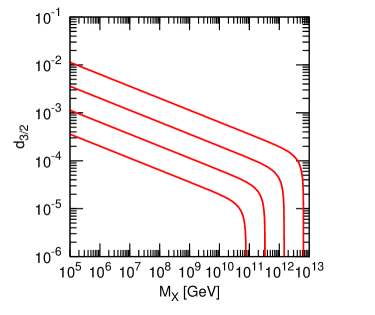
Figure 1: Contour plot of $Y_{3/2}$ in the plane of $M_{X}$ and $d_{3/2}$ when $\Gamma_{X}$ is given by Eq. (28) with $d_{\rm tot}=1$. The solid lines correspond to $Y_{3/2}=10^{-16}$, $10^{-15}$, $10^{-14}$ and $10^{-13}$ from left to right, respectively.

We first consider the unstable gravitino, especially when the gravitino mass lies in $M_{3/2}\sim 100$ GeV –$10$ TeV as suggested by the gravity mediation models of SUSY breaking. The heavy gravitino with $M_{3/2}\sim 1$ TeV decays soon after the BBN epoch. The decay rate of the gravitino into the MSSM particles is estimated as $\Gamma\simeq 193/(384\pi)M_{3/2}^{3}/M_{P}^{2}$, corresponding to the lifetime $\tau\simeq 2.4\times 10^{4}\mbox{sec}\,(1\mbox{TeV}/M_{3/2})^{3/2}$. In this case, the yield $Y_{3/2}$ is bounded from above, i.e. $Y_{3/2}<Y_{3/2}^{\rm BBN}$, in order to keep the success of the standard scenario of BBN Khlopov:1984pf . Otherwise, the decay products of the gravitino would change the abundances of primordial light elements too much and consequently conflict with the observational data. The recent analysis Kohri:2005wn shows that, when the hadronic branching ratio of the gravitino decay is of order unity, $Y_{3/2}^{\rm BBN}\sim 10^{-16}$ for $M_{3/2}\sim 1$ TeV and $Y_{3/2}^{\rm BBN}\sim 10^{-15}$–$10^{-13}$ for $M_{3/2}\sim 10$ TeV. The constraint disappears only when the gravitino mass is very heavy: $M_{3/2}\gtrsim 100$ TeV. We will not consider such a heavy gravitino, as the region $M_{3/2}\sim 10^{2}-10^{3}$ TeV is excluded by the overclosure of the LSPs Nakamura:2006uc and the allowed region with $M_{3/2}\gtrsim 10^{3}$ TeV is disfavored as the solution to the naturalness problem inherent to the weak scale.

The yield of the gravitinos produced by the thermal scatterings is estimated as Bolz:2000fu ; Kawasaki:2004qu

$$Y_{3/2}^{\rm TH}\simeq 1.1\times 10^{-12}\left(\frac{T_{R}}{10^{10}\mbox{GeV}}\right)\,,$$ (34)

which increases linearly as $T_{R}$ increases. On the other hand, the yield of the gravitinos by the $X$ decay is given by Eq. (32).

Consider the case where the $X$ field decays through Planck suppressed interaction, in which the total decay rate $\Gamma_{X}$ is given as Eq. (28) with $d_{\rm tot}={\cal O}(1)$. Then

$$Y_{3/2}^{\rm TH} \simeq 6.5\times 10^{-18}d_{\rm tot}\,\left(\frac{M_{X}}{10^{10}\mbox{GeV}}\right)^{\frac{3}{2}}\,,$$

$$Y_{3/2}^{X} \simeq 8.9\times 10^{-6}\,B_{3/2}d_{\rm tot}\,\left(\frac{M_{X}}{10^{10}\mbox{GeV}}\right)^{\frac{1}{2}}\,,$$ (35)

with the total abundance $Y_{3/2}=Y_{3/2}^{X}+Y_{3/2}^{\rm TH}$. In this case, $Y_{3/2}$ is determined by $M_{X}$ and $B_{3/2}$, and $Y_{3/2}^{X}\gtrsim Y_{3/2}^{\rm TH}$ for $M_{X}\lesssim 1.4\times 10^{10}(B_{3/2}/10^{-12})\;\mbox{GeV}$. In Fig. 1 we show the constant contours of $Y_{3/2}$ in the plane of $M_{X}$ and $d_{3/2}$. Here we have set $d_{\rm tot}=1$. It is seen that the mass $M_{X}$ (and hence $T_{R}$) is bounded from above by the BBN constraint $Y_{3/2}\simeq Y_{3/2}^{\rm TH}<Y_{3/2}^{\rm BBN}$. Moreover, in order to avoid the overproduction of the gravitinos by the $X$ decays, the coupling constant $d_{3/2}$ should satisfy

$$d_{3/2}\lesssim 2.0\times 10^{-5}d_{\rm tot}^{-\frac{1}{2}}\,\left(\frac{M_{X}}{10^{10}\mbox{GeV}}\right)^{-\frac{1}{4}}\left(\frac{Y_{3/2}^{\rm BBN}}{10^{-16}}\right)^{\frac{1}{2}}\,,$$ (36)

or equivalently

$$B_{3/2}\lesssim 1.1\times 10^{-11}d_{\rm tot}^{-1}\left(\frac{M_{X}}{10^{10}\mbox{GeV}}\right)^{-\frac{1}{2}}\left(\frac{Y_{3/2}^{\rm BBN}}{10^{-16}}\right)\,.$$ (37)

This gives a stringent constraint on the decay into the gravitino pair, or equivalently, the $F$-component VEV of the $X$ field. In fact, when the total decay rate is controlled by the Planck suppressed interaction ($d_{\rm tot}={\cal O}(1)$), this constraint excludes the case of $d_{3/2}={\cal O}(1)$ as far as the gravitino mass is $M_{3/2}\sim 100$ GeV–$10$ TeV. Thus, the cosmological moduli problem cannot be solved by simply raising the moduli mass Endo:2006zj ; Nakamura:2006uc . At the same time, the above constraint poses a severe restriction to inflation models. In particular, the modular inflation scenario where one of the moduli fields is used as the inflaton would face a serious difficulty.

The bound (36) also implies that the scalar decay survives the BBN constraint if $d_{3/2}$ is small and/or $d_{\rm tot}$ is large. The former can be achieved by some cancellation among the contributions in Eq. (11), or by the VEV of the $X$ field $\langle X\rangle$ smaller than the Planck scale. The latter can be achieved if the $X$ field has stronger interaction to the MSSM particles than the Planck suppressed one.

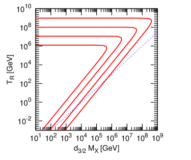
Figure 2: Contour plot of $Y_{3/2}$ in the plane of $d_{3/2}M_{X}$ and $T_{R}$. The solid lines correspond to $Y_{3/2}=10^{-16}$, $10^{-15}$, $10^{-14}$ and $10^{-13}$, from inside to outside, respectively. The dotted line is the lower bound on $T_{R}$ from $B_{3/2}\leq 1$ for $d_{3/2}=10^{-10}$.

To illustrate such a more general case, it may be convenient to use $T_{R}$ and take it as a free parameter. In this case, from Eqs. (2) and (27) the branching ratio $B_{3/2}$ is written as

$$B_{3/2}=\frac{d_{3/2}^{2}}{288\pi}\left(\frac{90}{\pi^{2}g_{\ast}(T_{R})}\right)^{\frac{1}{2}}\frac{M_{X}^{3}}{T_{R}^{2}M_{P}}\,,$$ (38)

where $B_{3/2}\leq 1$ as it should be. Then, $Y_{3/2}^{\rm TH}$ is given by Eq. (34), while $Y_{3/2}^{X}$ can be written by using Eq. (38) as

$$Y_{3/2}^{X}\simeq\frac{1}{192\pi}\left(\frac{90}{\pi^{2}g_{\ast}(T_{R})}\right)^{\frac{1}{2}}\frac{d_{3/2}^{2}M_{X}^{2}}{T_{R}M_{P}}\,.$$ (39)

Quite interestingly, $Y_{3/2}^{X}$ is inversely proportional to $T_{R}$, whereas $Y_{3/2}^{\rm TH}$ is proportional to $T_{R}$. This means that the BBN observation puts not only the upper bound but also the lower bound on the reheating temperature. Further, it is seen that the total yield $Y_{3/2}=Y_{3/2}^{X}+Y_{3/2}^{\rm TH}$ can be determined from two parameters, i.e. $d_{3/2}M_{X}$ and $T_{R}$. In Fig. 2 we draw the contour plot of $Y_{3/2}$ in the plane of $d_{3/2}M_{X}$ and $T_{R}$. Here we have fixed $g_{\ast}(T_{R})=200$, for simplicity. It is clearly seen that $Y_{3/2}^{\rm BBN}$ puts the upper bound on $d_{3/2}M_{X}$ as well as $T_{R}$. This bound can be found as follows: In general, $Y_{3/2}=Y_{3/2}^{X}+Y_{3/2}^{\rm TH}\geq 2\sqrt{Y_{3/2}^{X}Y_{3/2}^{\rm TH}}\equiv Y_{3/2}^{\rm MIN}$, where the equality holds when $Y_{3/2}^{X}=Y_{3/2}^{\rm TH}$, i.e., $T_{R}\simeq 1.2d_{3/2}M_{X}$ from Eqs. (34) and (39). It is obtained that

$$Y_{3/2}^{\rm MIN}\simeq 2.6\times 10^{-22}\,\mbox{GeV}^{-1}\,d_{3/2}M_{X}\,,$$ (40)

and hence $Y_{3/2}^{\rm MIN}<Y_{3/2}^{\rm BBN}$ gives the upper bound

$$M_{X}\lesssim 4\times 10^{5}\mbox{GeV}\,\frac{1}{d_{3/2}}\left(\frac{Y_{3/2}^{\rm BBN}}{10^{-16}}\right)\,.$$ (41)

Notice that we have assumed $M_{X}\gg M_{3/2}\sim 1$ TeV in this case. Therefore, when $d_{3/2}={\cal O}(1)$, this gives a sever bound on the mass of the scalar field $X$.

We should note that the parameter space in Fig. 2 may contradict $B_{3/2}\leq 1$. Indeed, the viable reheating temperature is

$$T_{R}\geq 10^{-5}\mbox{GeV}\,\frac{1}{d_{3/2}^{\frac{1}{2}}}\left(\frac{d_{3/2}M_{X}}{10^{4}\mbox{GeV}}\right)^{\frac{3}{2}}\,.$$ (42)

As an example, we also show in Fig. 2 this lower bound on $T_{R}$ for $d_{3/2}=10^{-10}$. It is thus found that the bound is insignificant as long as $d_{3/2}$ is sufficiently large.

Finally, when $Y_{3/2}=Y_{3/2}^{\rm MIN}$, the branching ratio is $B_{3/2}\simeq 1.8\times 10^{-4}M_{X}/M_{P}$ and then from Eq. (41) we find

$$d_{3/2}B_{3/2}\lesssim 2.9\times 10^{-17}\left(\frac{Y_{3/2}^{\rm BBN}}{10^{-16}}\right)\,.$$ (43)

This again tells that, in order to avoid the overproduction of the gravitinos, we have to require (i) very small $d_{3/2}$ and/or (ii) very small $B_{3/2}$. The former one may be realized by a VEV of $X$ much smaller than $M_{P}$, while the latter one may demand interactions of $X$ to the MSSM particles, whose strength is much larger than $1/M_{P}$, to increase $d_{\rm tot}$.

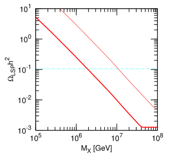
Figure 3: Present abundance of the wino LSP $\Omega_{\widetilde{W}}h^{2}$ when $\Gamma_{X}$ is given by Eq. (28) with $d_{\rm tot}=1$. The thick and thin solid lines are for $M_{\widetilde{W}}=100$ and 300 GeV, respectively. The horizontal dot-dashed line is the present dark matter density $\Omega_{\rm dm}h^{2}\simeq 0.105$.

Next, we would like to discuss an additional constraint concerning the abundance of the LSPs. The LSP is stable when the $R$-parity is conserved. To be consistent with the current observation of the cosmic microwave background radiation Spergel:2006hy , the present LSP abundance should be

$$\Omega_{\rm LSP}h^{2}\leq\Omega_{\rm dm}h^{2}=0.105^{+0.008}_{-0.014}\,,$$ (44)

where $h\simeq 0.73$ Spergel:2006hy is the present Hubble constant in the unit of 100km/sec/Mpc.

The LSP is produced by the decays of the gravitinos discussed above. We then obtain the upper bound on the yield of the gravitinos as

$$Y_{3/2}<3.8\times 10^{-12}\left(\frac{\Omega_{\rm dm}}{0.105}\right)\left(\frac{M_{\rm LSP}}{100\mbox{GeV}}\right)^{-1}\,,$$ (45)

with $M_{\rm LSP}$ being the LSP mass. We can see that the bound is much weaker than the constraint from the BBN ($Y_{3/2}^{\rm BBN}$), and it gives no additional bound. In addition, the LSP is produced directly by the $X$ decay Moroi:1994rs ; Kawasaki:1995cy ; Moroi:1999zb . Here we consider the neutral wino $\widetilde{W}$ as the LSP to maximize the annihilation cross section leading to the most conservative bound. The details of estimating the present abundance of $\widetilde{W}$ are found in Appendix A.

In Fig. 3 we show $\Omega_{\widetilde{W}}h^{2}$ in terms of $M_{X}$ by using Eq. (29). We find that $\Omega_{\widetilde{W}}h^{2}$ becomes constant for $M_{X}\gtrsim 4\times 10^{7}$ GeV for $M_{\widetilde{W}}=100$ GeV, while $\Omega_{\widetilde{W}}h^{2}$ becomes larger as $M_{X}$ decreases. (See the discussion in Appendix A). Therefore, we obtain the lower bound $M_{X}$ to avoid the overclosure by the wino LSP, and $M_{X}\gtrsim 2\times 10^{6}$ GeV for $M_{\widetilde{W}}=100$ GeV. The bound becomes more stringent for larger $M_{\widetilde{W}}$. For example, $M_{X}\gtrsim 10^{7}$ GeV for $M_{\widetilde{W}}=300$ GeV. On the other hand, when we take $T_{R}$ as a free parameter, $\Omega_{\widetilde{W}}h^{2}$ depends on $M_{X}$ as well as $T_{R}$. As estimated in Appendix A, the smaller values of $M_{X}$ and $T_{R}$ are excluded. This restricts the cosmologically viable parameters of the field $X$. Finally, we should notice that the bounds become severer when the LSP is composed of other neutralino components.

III.3 Stable gravitino

We now turn to the case of stable gravitino. This is the case when the gravitino is the LSP with exact $R$-parity conservation. In this situation, the present abundance of the gravitinos is bounded from above in order to avoid the overclosure of the universe Pagels:1981ke ; Moroi:1993mb . For this reason, let us estimate the density parameter of the gravitinos, which is given by the present energy density of the gravitino divided by the critical density $\rho_{\rm cr}$. The present abundance of the gravitinos produced by the thermal scatterings is given by Bolz:2000fu

$$\Omega_{3/2}^{\rm TH}h^{2}\simeq 0.21\left(\frac{T_{R}}{10^{10}\mbox{GeV}}\right)\left(\frac{M_{3/2}}{100\mbox{GeV}}\right)^{-1}\,.$$ (46)

Note that $\Omega_{3/2}^{\rm TH}$ is dominated by the contribution from the helicity 1/2 components of gravitino and it is inversely proportional to $M_{3/2}$. On the other hand, for the gravitinos from the $X$ decay, we find from Eq. (32) that

$$\Omega_{3/2}^{X}=\frac{M_{3/2}Y_{3/2}^{X}}{\rho_{\rm cr}/s_{0}}=\frac{0.027}{h^{2}}\left(\frac{M_{3/2}}{1\mbox{GeV}}\right)\left(\frac{Y_{3/2}^{X}}{10^{-10}}\right)\,,$$ (47)

where $s_{0}$ is the present entropy density and $\rho_{\rm cr}/s_{0}\simeq 3.6\times 10^{-9}$ $h^{2}$ GeV. Thus, the total abundance is $\Omega_{3/2}=\Omega_{3/2}^{X}+\Omega_{3/2}^{\rm TH}$. To avoid the overclosure by gravitinos, we must require

$$\Omega_{3/2}h^{2}\leq\Omega_{\rm dm}h^{2}\,.$$ (48)

Especially, when $\Omega_{3/2}=\Omega_{\rm dm}$, the gravitinos constitutes the dark matter of the universe. As seen from Eq. (47), the bound on $Y_{3/2}^{X}$ in the present case is much weaker than that from the BBN for unstable gravitinos.

Furthermore, we have to take into account an additional constraint. Indeed, the gravitinos produced by the $X$ decay face a constraint from the cosmic structure formation. Since the momentum of the gravitino at the production ($p\simeq M_{X}/2$) can be much larger than its mass, its free-streaming at the epoch of the matter-radiation equality may erase the small scale structures which are observed today. This warm dark matter constraint leads to the upper bound on the present velocity dispersion of the gravitino $v_{0}$ Jedamzik:2005sx . The power spectrum inferred from the Ly-$\alpha$ forest data together with the cosmic microwave background radiation and galaxy clustering constraints puts severe limits Viel:2005qj ; Seljak:2006qw . From Ref. Seljak:2006qw we find approximately $v_{0}\lesssim 4\times 10^{-8}$. On the other hand, the present velocity of gravitinos produced by the $X$ decay is estimated as

$$v_{0}=\frac{1}{2}\left(\frac{g_{\ast s}(T_{0})}{g_{\ast s}(T_{R})}\right)^{\frac{1}{3}}\sqrt{1-\frac{4M_{3/2}^{2}}{M_{X}^{2}}}\frac{T_{0}M_{X}}{M_{3/2}T_{R}}\,,$$ (49)

where $T_{0}=2.35\times 10^{-13}$ GeV is the present photon temperature and $g_{\ast s}(T_{0})=43/11$. Using Eqs. (32) and (47), we find that

$$\Omega_{3/2}^{X}\simeq\frac{3B_{3/2}}{2}\frac{M_{3/2}T_{R}}{M_{X}(\rho_{\rm cr}/s_{0})}\,.$$ (50)

Therefore, $v_{0}$ can be written as

$$v_{0}\simeq 1.2\times 10^{-4}\,B_{3/2}\,,$$ (51)

where we assume that $\Omega_{3/2}^{X}h^{2}=\Omega_{\rm dm}h^{2}\simeq 0.105$. Thus, the warm dark matter constraint on the gravitinos is translated to the upper bound on the branching ratio as

$$B_{3/2}\lesssim 3\times 10^{-4}\,.$$ (52)

It should be noted that this warm dark matter constraint can become weaken, as the portion of the gravitino dark matter in the whole dark matter density becomes smaller. Ref. Viel:2005qj gives the upper bound to $\Omega_{3/2}^{X}\lesssim 0.12\;\Omega_{\rm dm}$ to eliminate the warm dark matter constraint. Here we shall use this as a representative bound.

Another potential constraint comes from the BBN, since additional energy from the gravitinos by the $X$ decay may increase the Hubble expansion rate at $T\sim 1$ MeV too much, which results in the overproduction of ⁴He. The bound, however, is rather weak: $B_{3/2}\lesssim 0.35$.

Let us first consider the case where the $X$ decays through the Planck suppressed interaction and the total decay rate of $X$ is given by Eq. (28). In this case, we find from Eqs. (46) and (47) that

$$\Omega_{3/2}^{\rm TH}h^{2} \simeq 3.9\times 10^{-2}d_{\rm tot}$$ (53)

$$\times\left(\frac{M_{X}}{10^{11}\mbox{GeV}}\right)^{\frac{3}{2}}\left(\frac{M_{3/2}}{0.1\mbox{GeV}}\right)^{-1}\,,$$

$$\Omega_{3/2}^{X}h^{2} \simeq 2.5\times 10^{-1}d_{\rm tot}\left(\frac{B_{3/2}}{10^{-4}}\right)$$ (54)

$$\times\left(\frac{M_{X}}{10^{11}\mbox{GeV}}\right)^{\frac{1}{2}}\left(\frac{M_{3/2}}{0.1\mbox{GeV}}\right)\,.~{}~{}~{}$$

Notice that $T_{R}$ is determined from $M_{X}$ as shown in Eq. (29). In Fig. 4 we show the contour lines of $\Omega_{3/2}h^{2}=0.105$ in the plane of $M_{3/2}$ and $M_{X}$ by varying $B_{3/2}$. It should be noted that $\Omega_{3/2}^{\rm TH}\propto M_{3/2}^{-1}$ while $\Omega_{3/2}^{X}\propto M_{3/2}$. Therefore, for the heavier gravitino mass region, $\Omega_{3/2}^{X}\gg\Omega_{3/2}^{\rm TH}$ and the gravitinos produced by the $X$ decay contribute significantly the present energy of the universe. It is clearly seen that one can escape the overclosure of the if the mass $M_{X}$ (and hence $T_{R}$) is sufficiently small. The upper bound on $M_{X}$ scales as $M_{3/2}^{\frac{2}{3}}$ for $\Omega_{3/2}\simeq\Omega_{3/2}^{\rm TH}$ with smaller gravitino masses, whereas it scales as $M_{3/2}^{-2}$ for $\Omega_{3/2}\simeq\Omega_{3/2}^{X}$ with heavier gravitino masses. When $B_{3/2}\gtrsim 3\times 10^{-4}$, the upper bound on $M_{X}$ becomes more stringent due to the warm dark matter constraint (see Fig. 4).

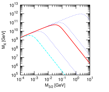
Figure 4: Upper bounds on $M_{X}$ in terms of $M_{3/2}$, when $\Gamma_{X}$ is given by Eq. (28) with $d_{\rm tot}=1$. The dotted lines correspond to the upper bounds from $\Omega_{3/2}h^{2}\leq\Omega_{\rm dm}h^{2}=0.105$ for $B_{3/2}=10^{-2}$, $10^{-4}$ and $10^{-6}$ from left to right, respectively. The solid line is the bound from $\Omega_{3/2}\leq\Omega_{\rm dm}$ for $B_{3/2}=3\times 10^{-4}$, and the gravitino dark matter becomes viable above this line. The dot-dashed line is the upper bound on $M_{X}$ from $\Omega_{3/2}^{X}\leq 0.12\Omega_{\rm dm}$ avoiding the warm dark matter constraint in addition to $\Omega_{3/2}\leq\Omega_{\rm dm}$, when $B_{3/2}=10^{-2}$.

We should stress here that the cosmological moduli problem can be solved in the small gravitino mass region. We expect for moduli fields that $B_{3/2}\sim 10^{-2}$ from $d_{3/2}={\cal O}(1)$ and $d_{\rm tot}={\cal O}(1)$. Even in this case, there indeed exists the parameter space avoiding cosmological difficulties of gravitinos, where the gravitino mass is $M_{3/2}\lesssim 0.1$ GeV and the moduli ($X$) mass is $M_{X}\sim 10^{5}$–$10^{9}$ GeV, corresponding to $10^{4}\;\mbox{GeV}\gtrsim T_{R}\gtrsim 7$ MeV. Here the lower bound on $M_{X}$ comes from Eq. (30), whereas the upper bound is due to the warm dark matter constraint. The required large hierarchy between $M_{3/2}$ and $M_{X}$ can be realized in a class of models of moduli stabilization. (See, for instance, Ref. Kallosh:2004yh .)

Here we would like to point out that the heavy scalar $X$ decay into a pair of gravitinos can offer an interesting and alternative window of dark matter. When $B_{3/2}\lesssim 3\times 10^{-4}$, the free-streaming effect of the produced gravitino is small so that the gravitino can constitute the dark matter of the universe, i.e. $\Omega_{3/2}^{\rm X}=\Omega_{\rm dm}$. In Fig. 4 we present the contour line of $\Omega_{3/2}h^{2}=0.105$ with $B_{3/2}=3\times 10^{-4}$ by the solid line. In the region above this line, the gravitino from the $X$ decay can become the viable dark matter as long as $\Omega_{3/2}^{X}=\Omega_{\rm dm}$.

We should mention that the properties of the gravitino dark matter can be different for different choices of parameters. Namely, the gravitino becomes the warm dark matter for $B_{3/2}\sim 3\times 10^{-4}$, and it gets cooler and eventually becomes the cold dark matter as the branching ratio decreases. Furthermore, the mixed scenario of cold and warm dark matter is possible. In particular, the gravitinos produced by $X$ can compose the warm component while those from the thermal scatterings can compose the cold one. More precise observations on the small scale structures of the universe enable us to test these hypotheses.

The small branching ratio $B_{3/2}\sim 10^{-4}$ indicates from Eq. (31) that $d_{3/2}\sim 0.1d_{\rm tot}$. Though for the moduli fields a naive expectation will be $d_{3/2}\sim d_{\rm tot}$, the suppression of one order of magnitude may also be possible in some moduli stabilization mechanism. If it is the case, the decays of the moduli field with mass of ${\cal O}(10^{9})$–${\cal O}(10^{11})$ GeV will yield the gravitino warm dark matter.

So far, we have assumed that the total decay rate of the $X$ field is given by Eq. (28) with $d_{\rm tot}$ not very for from unity. Now we take $\Gamma_{X}$ or $T_{R}$ as a free parameter. Notice that we find from Eq. (38) that

$$M_{X} = \left(\frac{288\pi}{d_{3/2}^{2}}\right)^{\frac{1}{3}}\left(\frac{\pi^{2}g_{\ast}(T_{R})}{90}\right)^{\frac{1}{6}}B_{3/2}^{\frac{1}{3}}\,T_{R}^{\frac{2}{3}}\,M_{P}^{\frac{1}{3}}\,,$$ (55)

which leads to

$$\Omega_{3/2}^{X}h^{2} = 4.1\times 10^{-2}\,\left(\frac{d_{3/2}B_{3/2}}{10^{-6}}\right)^{\frac{2}{3}}$$ (56)

$$\times\left(\frac{T_{R}}{10^{4}\mbox{GeV}}\right)^{\frac{1}{3}}\left(\frac{M_{3/2}}{1\mbox{GeV}}\right)\,.$$

The total abundance $\Omega_{3/2}=\Omega_{3/2}^{X}+\Omega_{3/2}^{\rm TH}$ is then determined by the two parameters, $T_{R}$ and $d_{3/2}B_{3/2}$, when the gravitino mass $M_{3/2}$ is given.

Similar to the case with unstable gravitino, we can obtain the upper bound on $d_{3/2}M_{X}$ to avoid the overclosure by gravitinos. Since $\Omega_{3/2}\geq\Omega_{3/2}^{\rm MIN}=2\sqrt{\Omega_{3/2}^{X}\Omega_{3/2}^{\rm TH}}$, $\Omega_{3/2}^{\rm MIN}h^{2}<\Omega_{\rm dm}h^{2}\simeq 0.105$ results in the bound

$$M_{X}\lesssim 5.7\times 10^{9}\mbox{GeV}\,\frac{1}{d_{3/2}}\,.$$ (57)

Further, if the branching ratio becomes larger than Eq. (52), this upper bound becomes tighter due to the warm dark matter constraint. We can see the bound is much weaker than Eq. (41) in the case of unstable gravitino.

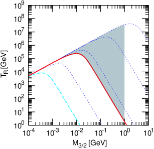
Figure 5: Upper bounds on $T_{R}$ in terms of $M_{3/2}$. The dotted lines correspond to the upper bounds from $\Omega_{3/2}h^{2}\leq\Omega_{\rm dm}h^{2}=0.105$ for $d_{3/2}B_{3/2}=10^{-2}$, $10^{-4}$, $10^{-6}$ and $10^{-8}$ from left to right, respectively. The solid line is the bound from $\Omega_{3/2}\leq\Omega_{\rm dm}$ for $d_{3/2}B_{3/2}=3\times 10^{-4}$, and the gravitino dark matter becomes viable above this line shown as the shaded region. The dot-dashed line is the upper bound on $T_{R}$ from $\Omega_{3/2}^{X}\leq 0.12\Omega_{\rm dm}$ avoiding the warm dark matter constraint in addition to $\Omega_{3/2}\leq\Omega_{\rm dm}$, when $d_{3/2}B_{3/2}=10^{-2}$.

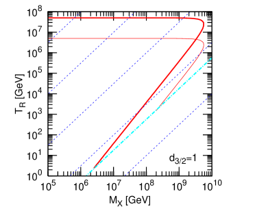
Figure 6: Allowed parameters for the gravitino dark matter with $M_{3/2}=1$ GeV (the thick solid line) and $M_{3/2}=0.1$ GeV (the thin solid line) when $d_{3/2}=1$. Contour lines of the branching ratio are shown by the dotted lines, which correspond to $B_{3/2}=1$, $10^{-5}$, $10^{-10}$, $10^{-15}$ and $10^{-20}$ from below, respectively. The upper bound on $B_{3/2}$ from the cosmic structure formation is shown by the dot-dashed line.

In Fig. 5, we show the contour plot of $\Omega_{3/2}=\Omega_{\rm dm}$ in the plane of $M_{3/2}$ and $T_{R}$ by varying $d_{3/2}B_{3/2}$. Notice that the upper bound on $B_{3/2}$ (52) can be applied even in the general case, and hence we expect $d_{3/2}B_{3/2}\lesssim 3\times 10^{-4}$ since $d_{3/2}\lesssim{\cal O}(1)$. In Fig. 5 we also show $\Omega_{3/2}h^{2}\simeq 0.105$ with $d_{3/2}B_{3/2}=3\times 10^{-4}$. Moreover, the upper bound on $T_{R}$ from the warm dark matter constraint is also shown when $d_{3/2}B_{3/2}=10^{-2}$. We find that the allowed region is similar to that in Fig. 4, but the dark matter window for the gravitinos produced by the $X$ decay is enlarged.

Further, we show in Fig. 6 the allowed parameter set of the gravitino dark matter for $d_{3/2}=1$ by taking the gravitino mass as $M_{3/2}=1$ GeV and 0.1 GeV. For smaller $d_{3/2}$, the corresponding branching ratio becomes smaller as shown in Eq. (38). It can be seen that the gravitino dark matter is possible in a wide range of parameter space, and an important implication is that $X$ should have the suppressed branching ratio of the decay into a pair of gravitinos as shown in Eq. (52).

Finally, we should argue that the NLSP (next-to-LSP) decay into gravitino restricts the allowed parameter space. Here let us consider, as an example, the case when a (right-handed) scalar tau $\widetilde{\tau}$ is the NLSP. The lifetime of $\widetilde{\tau}\to\psi_{3/2}+\tau$ is

$$\tau_{\widetilde{\tau}}\simeq 5.9\times 10^{4}\mbox{sec}\left(\frac{M_{3/2}}{1\mbox{GeV}}\right)^{2}\left(\frac{M_{\widetilde{\tau}}}{100\mbox{GeV}}\right)^{-5}\,,$$ (58)

and $\widetilde{\tau}$ decays during the BBN period or later for $M_{3/2}\gtrsim 10$ MeV when we take, e.g., $M_{\widetilde{\tau}}=100$ GeV. Therefore, when the gravitino mass is sufficiently small, the $\widetilde{\tau}$ NLSP becomes cosmologically harmless. On the other hand, when the gravitino mass becomes larger, the decay products would dissociate or overproduce the light elements synthesized at the BBN epoch and would conflict with the observations. To avoid this, the number of $\widetilde{\tau}$ at the decay time should be small enough. In Appendix A, we estimate the abundance of $\widetilde{\tau}$, $Y_{\widetilde{\tau}}$ in terms of $M_{X}$ and $T_{R}$.

The BBN constraint on $Y_{\widetilde{\tau}}$ ($M_{\widetilde{\tau}}Y_{\widetilde{\tau}}$ more precisely) strongly depends on how $\widetilde{\tau}$ decays into hadrons Kawasaki:2004qu ; Kohri:2005wn ; Feng:2004zu . According to the hadronic branching ratio $B_{h}$ in Ref. Feng:2004zu and also to the BBN constraints for $B_{h}=1$ and $10^{-3}$ in Ref. Kawasaki:2004qu , we find that two regions, $\tau_{\widetilde{\tau}}\lesssim 10^{2}$ sec and $10^{6}$ sec $\gtrsim\tau_{\widetilde{\tau}}\gtrsim 10^{3}$ sec, are cosmologically viable. Here we have used $Y_{\widetilde{\tau}}\sim 10^{-13}$ by assuming that the reheating temperature $T_{R}$ is higher than the freeze-out temperature of the stau annihilation, $T_{F}$(see the discussion in Appendix). Although we cannot find the relevant constraint for $10^{3}$ sec $\gtrsim\tau_{\widetilde{\tau}}\gtrsim 10^{2}$ sec (i.e. $B_{h}=10^{-3}$–1) in the literature, we consider such a window is also allowed from the rough estimate of the BBN constraints interpolating in the region $B_{h}=10^{-3}$–1. In this analysis, therefore, we take $\tau_{\widetilde{\tau}}\lesssim 10^{6}$ sec as a representative bound, which leads to $M_{3/2}\lesssim 4\mbox{GeV}$ for $M_{\widetilde{\tau}}$. We should stress here that our final conclusions leave intact even when the bound on $\tau_{\widetilde{\tau}}$ becomes severer. Since the lifetime of $\widetilde{\tau}$ depends on $M_{\widetilde{\tau}}^{5}$, the upper bound on $M_{3/2}$ can be enlarged by larger $M_{\widetilde{\tau}}$. Finally, this analysis is true for $T_{R}\gtrsim T_{F}$. On the other hand, for $T_{R}\lesssim T_{F}$, the bound on $M_{3/2}$ becomes stronger or weaker in the low or high $M_{X}$ region, respectively. The bottom line is that the BBN constraint on the $\widetilde{\tau}$ NLSP decay can be escaped for $M_{3/2}<{\cal O}(1)$ GeV at least when the reheating temperature is higher than about $T_{F}$. The detail analysis in other parameter space will be done in future publication.

The upper bound on the gravitino mass of $M_{3/2}\lesssim{\cal O}(1)$ GeV implies that the maximal reheating temperature is $T_{R}\simeq 5\times 10^{7}$ GeV. Such a high reheating temperature is possible only when $B_{3/2}\lesssim 10^{-6}$ such that $\Omega_{3/2}\simeq\Omega_{3/2}^{\rm TH}$. For larger $B_{3/2}$ the upper bound on $T_{R}$ is suppressed due to the gravitino production from the $X$ decay. Note that the upper bound on $T_{R}$ is directly translated into the upper bound on $M_{X}$ through Eq. (29). For instance, $T_{R}\lesssim 5\times 10^{7}$ GeV gives $M_{X}\lesssim 9\times 10^{11}$ GeV for $d_{\rm tot}=1$. (Note that $M_{X}\gtrsim 1.5\times 10^{5}$ GeV to have $T_{R}\gtrsim 7$ MeV.)

IV Conclusions and Discussion

In this paper, we have considered the cosmological implications to the decay of the general heavy scalar field into the gravitino pair. Here we would like to summarize what we have obtained in this analysis.

As was shown in the previous works Endo:2006zj ; Nakamura:2006uc , the decay amplitude to the gravitino pair is proportional to the VEV of the auxiliary component $\langle F^{X}\rangle$ of the heavy field $X$. We have thus presented the estimate for the VEV of $F^{X}$ in a general setting: we have considered the general coupling between $X$ and the fields responsible for the spontaneous supersymmetry breaking, and also we have considered the case of the explicit supersymmetry breaking as well. In both cases, we have obtained the same and simple estimate for this value when only a single $X$ field participates. The result shows that generally the VEV of $F^{X}$ is proportional to the VEV of the $X$ field, and thus the partial decay rate into the gravitino pair is suppressed when the $X$’s VEV is smaller than the Planck scale.

We have then considered the various constraints on the gravitino production at the decay of the heavy scalar field $X$. The relevant constraints are different whether the gravitino is stable or not, and so we have discussed the two cases separately. In the unstable gravitino case, the constraints we have considered are

1. The BBN constraint on the decay of the gravitinos, producing hadronic as well as electromagnetic activities.

2. The constraint on the abundance of the LSPs produced at the gravitino decay.

3. The constraint on the abundance of the LSPs produced directly at the $X$ decay.

It is well-known that the BBN constraint puts the upper bound on the reheat temperature $T_{R}$ in order to suppress the gravitino yield produced by the thermal scatterings Khlopov:1984pf . In the case at hand, the decay of the $X$ field produces the gravitinos as well. Since its yield becomes larger when we lower the reheat temperature, the BBN bound gives the lower bound on $T_{R}$. We have identified the allowed range of $T_{R}$ both in the case where the $X$ field is moduli-like and in the more general case. We have confirmed that if the gravitino mass lies in 100 GeV–10 TeV range, no allowed region exists when $S$ is a moduli-like field, namely the field whose the decay into gravitinos is not suppressed ($d_{3/2}={\cal O}(1)$) and the decay into other particles is controlled by the Planck suppressed interaction ($d_{\rm tot}={\cal O}(1)$). On the other hand, for a more general case, we have found that the viable region of the parameter space does exist, but is severely constrained, as was shown in Fig. 2.

We have seen that the second constraint is weaker than the first one, provided that the gravitino mass is in the range given above. On the contrary, the third constraint excludes the case of very low reheat temperature, as the annihilation processes of the neutralino LSPs are not very effective there and thus the LSP abundance exceeds the observational abundance of the dark matter in the universe.

For the stable gravitino case, we have discussed the following constraints:

1. The constraint on the gravitino abundance to avoid the overclosure of the universe.

2. The constraint from the warm dark matter, namely the free streaming of the gravitino produced by the heavy $X$ decay is small enough for the gravitino to be a viable warm dark matter.

3. The BBN constraint on the decay of the NLSP particles into the gravitinos.

The first constraint is similar to the first one in the unstable gravitino case, but numerically in the stable gravitino case it is less severe. This makes a wider region of the parameter space cosmologically viable. In particular the constraint on the gravitino abundance allows the moduli-like scalar field when the gravitino mass is lighter than 1-100 MeV, depending on the mass of the $X$ field.

The second constraint given in the above list also gives a significant constraint. We have found that it puts the upper bound on the branching ratio as $B_{3/2}\lesssim 3\times 10^{-4}$ when the gravitino warm dark matter is the dominant component of the dark matter. This constraint disappears if the gravitino dark matter contribution less than 12% of the total dark matter density.

The third constraint is also quite stringent, but rather involved. With the lack of the complete analysis all through the relevant parameter regions, we have argued to put the upper bound on the gravitino mass (or the lifetime of the NLSP) as roughly of order 1 GeV when the NLSP is the stau weighing 100 GeV.

In the rest of the paper, we would like to discuss the implications of our results to the inflationary scenarios. Assuming that there is no entropy production at a later epoch, our consideration gives a stringent constraint on the reheating process right after the inflation. When the inflaton is one of the moduli fields Blanco-Pillado:2004ns ; Blanco-Pillado:2006he ; Lalak:2005hr , and the oscillating field is in fact moduli-like, then our results severely constrain the allowed gravitino mass region. In particular for the unstable gravitino, the analysis in Ref. Nakamura:2006uc can apply, leaving only the very heavy gravitino, e.g. for the wino LSP $M_{3/2}\gtrsim 10^{3}$ TeV, which is disfavored as the solution to the naturalness problem on the weak scale. On the other hand, the case of a light and stable gravitino becomes cosmologically viable (see Fig. 5). However the low reheat temperature is required to suppress the gravitino abundance produced through thermal scattering, which may be inconsistent with a class of modular inflation with inflaton mass around $10^{10}$ GeV. It is interesting to note that a new window of the gravitino warm dark matter opens up in which the gravitino with the mass around 100 MeV, produced by the heavy moduli decay, constitutes the warm dark matter. Furthermore the reheat temperature is of the order $10^{5}$ GeV, which is a natural range we expect with the modular inflaton mass given above. The price we have to pay to realize this fascinating case is a slight suppression of the parameter $d_{3/2}$ by one order of magnitude, which, we suspect, should be possible within the framework of modular inflation.

As an important remark, we would like to emphasize that the above argument to the modular inflation can also apply to the cosmological moduli problem. In the unstable gravitino case, the cosmological constraints are too strong to be escaped unless the gravitino mass is heavier than, say, $10^{3}$ TeV as was discussed above. On the contrary, the cosmological moduli problem can be solved when the gravitino is light and stable, say $M_{3/2}\lesssim 0.1$ GeV. Such light gravitinos can be realized in the models of the gauge-mediated supersymmetry breaking. Compared to the modular inflation where the $X$ mass is rather high, it is anticipated that the moduli mass is not very far from the electroweak scale. Thus somewhat different region in the parameter space may be favored. For instance, the $X$ mass much below $10^{10}$ GeV is also fine in this case. Anyway, the solution requires the large hierarchy between masses $M_{3/2}$ and $M_{X}$, which can be realized in a class of models of the moduli stabilization Kallosh:2004yh .

Let us come back to the implications to the inflationary models. Our results given in Section 3 indicate that, to make the inflaton decay cosmologically viable in a wider range of the parameter space, a smaller branching ratio of the decay into the gravitino pair (a smaller $d_{3/2}$) and a larger total decay rate (a larger $d_{\rm tot}$) is favored. In a simple class of the chaotic inflation, the Lagrangian is invariant under a $Z_{2}$ discrete symmetry, a reflection of the field variable $X\to-X$. Thus at the minimum of the vacuum, $F_{X}$ will vanish and thus the decay of the inflaton into the gravitino pair does not take place and so the model does not suffer from the gravitino production problem. There are other inflationary models in which the parameter $d_{3/2}$ becomes much smaller than unity, by realizing the VEV of $X$ in an intermediate scale lower than the Planck scale. Examples include a new inflation model and also a hybrid inflation. Whether these models are really viable or not require detailed case study. A consideration can be found in Ref. Kawasaki:2006gs .

Finally to make $d_{\rm tot}$ large, one can construct an inflation model where the inflaton interacts to other particles with renormalizable couplings. An example is given as follows. Suppose an inflaton $X$ couples to a pair of right-handed neutrinos in the superpotential as $W=(f_{N}/2)XN^{c}N^{c}$, where $f_{N}$ is a coupling constant and the Majorana mass of $N^{c}$ is given by $M_{N}=f_{N}\langle X\rangle$. Now, we set $\langle X\rangle=10^{15}$ GeV. In this case, we find $B_{3/2}\sim 10^{-9}$ from the decay rate in Eq. (28). The inflaton decay rate of $\Phi\to N^{c}+N^{c}$ is $\Gamma_{N^{c}}=M_{N}^{2}M_{X}/(32\pi)/\langle X\rangle^{2}$, which becomes much larger in some parameter region. For example, $B_{3/2}\sim 10^{-12}$ for $M_{X}=10^{10}$ GeV and $M_{N}=10^{9}$ GeV by taking $d_{3/2}=\langle X\rangle/M_{P}$. Due to this fact, the cosmological constraints become weaker.

Appendix A

In this appendix, we briefly explain an estimation of the abundance of the lightest superparticle in the MSSM, which is denoted by $A$. In the text, we consider $A$ as the neutral wino for unstable gravitinos, while $A$ as the stau for stable gravitinos.

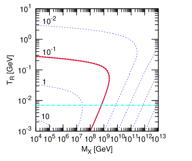
Figure 7: Contour plot of the present abundance of the wino LSP $\Omega_{\widetilde{W}}h^{2}$ for $M_{\widetilde{W}}=100$ GeV. The dotted lines are $\Omega_{\widetilde{W}}h^{2}=10$, 1, …, $10^{-5}$ from left to right, respectively. For $T_{R}\gtrsim 10$ GeV, $\Omega_{\widetilde{W}}h^{2}\simeq 1.3\times 10^{-3}$. The solid line shows $\Omega_{\widetilde{W}}h^{2}=0.105$, and the left-bottom region is excluded by the overclosure by $\widetilde{W}$. The horizontal dot-dashed line represents the lower bound on $T_{R}(\gtrsim 7$MeV).

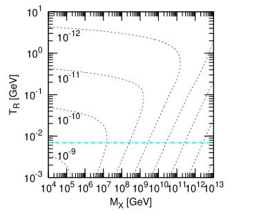
Figure 8: Contour plot of $Y_{\widetilde{\tau}}$ in the $M_{X}$-$T_{R}$ plane for $M_{\widetilde{\tau}}=100$ GeV. The dotted lines correspond to $Y_{\widetilde{\tau}}$ = $10^{-9}$–$10^{-16}$ from left to right. For $T_{R}\gtrsim 10$ GeV, $Y_{\widetilde{\tau}}\simeq 1.2\times 10^{-13}$. The horizontal dot-dashed line represents the lower bound on $T_{R}(\gtrsim 7$MeV).

The decay of $X$ and also the thermal scatterings produce $A$, and then the number density of $A$, $n_{A}$, can be found by solving the following coupled equations (see, for example, Ref. Gelmini:2006pw and the references therein);

$$\dot{\rho}_{X}+3H\rho_{X}=-\Gamma_{X}\rho_{X}\,,$$ (59)

$$\dot{\rho}_{R}+4H\rho_{R}=+\Gamma_{X}\rho_{X}\,,$$ (60)

$$\dot{n}_{A}+3Hn_{A}=\langle\sigma v\rangle\left(n_{\rm eq}^{2}-n_{A}^{2}\right)+\frac{B_{A}\,\Gamma_{X}}{M_{X}}\rho_{X}\,,~{}~{}$$ (61)

where $\rho_{X}$ and $\rho_{R}$ are the energy densities of the $X$ field and radiations, respectively, and the dot denotes a time derivative. $M_{X}$ and $\Gamma_{X}$ are the mass and total decay rate of $X$. $B_{A}$ denotes the effective number of $A$ per a $X$ decay. $\langle\sigma v\rangle$ are the annihilation cross section which is thermally averaged, and $n_{\rm eq}$ is the equilibrium value of the number density of $A$. In these equations, $H$ is the Hubble expansion rate which is given by $H^{2}=(\rho_{X}+\rho_{R})/(3M_{P}^{2})$. The cosmic temperature is found from $\rho_{R}$. Here we have neglected the co-annihilation effects on $n_{A}$, and the contribution to $\rho_{R}$ from $A$ since it can be negligible, and also assumed the rapid thermalization of $A$ just after the production Kawasaki:1995cy ; Hisano:2000dz .

In solving these equations, we assume that the energy of the universe is dominated by $X$ for $H>\Gamma_{X}$, and we take the initial condition such that the maximal temperature of the dilute plasma (for $H>\Gamma_{X}$) becomes sufficiently high to keep $A$ in the thermal equilibrium. The decay rate $\Gamma_{X}$ is parameterized by the reheating temperature $T_{R}$ as

$$\Gamma_{X}=\left(\frac{\pi^{2}g_{\ast}(T_{R})}{90}\right)^{\frac{1}{2}}\frac{T_{R}^{2}}{M_{P}}\,.$$ (62)

The abundance of $A$ is determined from two parameters $T_{R}$ and $B_{A}/M_{X}$, in addition to $\langle\sigma v\rangle$ and $M_{A}$. For simplicity, we shall take $B_{A}=0.5$ in this analysis, and the results for other values of $B_{A}$ can be found by the rescaling of $M_{X}$ as long as $T_{R}$ is considered as a free parameter. Then, $T_{R}$ and $M_{X}$ control the abundance of $A$, i.e. the yield of $A$, $Y_{A}$, after $A$ decouples from the thermal bath.

When $T_{R}\gtrsim T_{F}$ ($T_{F}$ is the freeze-out temperature of $A$ and $T_{F}\sim M_{A}/20$), $Y_{A}$ does not depend on $M_{X}$. This is because $A$ is still in the equilibrium after the decay of $X$ completes, and its abundance is evaluated from $\langle\sigma v\rangle$ and $M_{A}$ as usual. On the other hand, when $T_{R}\lesssim T_{F}$, $Y_{A}$ strongly depends on $T_{R}$ and $M_{X}$. When $M_{X}$ is sufficiently small, $A$ is produced so abundantly by the $X$ decays due to the source term in Eq. (61) that $Y_{A}$ is determined by its annihilation effect at $H\sim\Gamma_{X}$. In this case, $Y_{A}$ is inversely proportional to $T_{R}$. On the other hand, when $M_{X}$ is sufficiently large, the annihilation at $H\sim\Gamma_{X}$ becomes insignificant and $Y_{A}$ is determined from the contributions from the production by thermal scatterings in the dilute plasma and also from the $X$ decay at $H\sim\Gamma_{X}$. In this case, we find that $Y_{A}\propto T_{R}$.

Now we present our numerical results. First, we consider the case when $A$ is the neutral wino $\widetilde{W}$ which is the stable LSP. In this case, we use Moroi:1999zb

$$\langle\sigma v\rangle=\frac{g_{W}^{4}(1-x_{W})^{\frac{3}{2}}}{2\pi(2-x_{W})^{2}}\frac{1}{M_{\widetilde{W}}^{2}}\,,$$ (63)

where $g_{W}$ is the weak gauge coupling and $x_{W}=M_{W}^{2}/M_{\widetilde{W}}^{2}$. In Fig. 7 we show the contour plot of the present abundance $\Omega_{\widetilde{W}}h^{2}=M_{\widetilde{W}}Y_{\widetilde{W}}h^{2}/(\rho_{\rm cr}/s_{0})$ by taking $M_{\widetilde{W}}=100$ GeV. For $T_{R}\gtrsim 10$ GeV, $\Omega_{\widetilde{W}}h^{2}$ takes a value of $1.3\times 10^{-3}$.

When $A$ is the stau $\widetilde{\tau}$ which is the NLSP, we use Asaka:2000zh

$$\langle\sigma v\rangle=\frac{4\pi\alpha_{em}^{2}}{M_{\widetilde{\tau}}^{2}}\,.$$ (64)

In Fig. 8 we show the contour plot of the yield $Y_{\widetilde{\tau}}$ by taking $M_{\widetilde{\tau}}=100$ GeV. For $T_{R}\gtrsim 10$ GeV, $Y_{\widetilde{\tau}}$ takes a value of $1.9\times 10^{-13}$.

References

-
(1)
A. D. Linde,
Phys. Lett. B 108, 389 (1982);
A. Albrecht and P. J. Steinhardt, Phys. Rev. Lett. 48, 1220 (1982). -
(2)
G. D. Coughlan, W. Fischler, E. W. Kolb, S. Raby and G. G. Ross,
Phys. Lett. B 131, 59 (1983)
T. Banks, D. B. Kaplan and A. E. Nelson, Phys. Rev. D 49, 779 (1994) [arXiv:hep-ph/9308292];
B. de Carlos, J. A. Casas, F. Quevedo and E. Roulet, Phys. Lett. B 318, 447 (1993) [arXiv:hep-ph/9308325]. - (3) M. Endo, K. Hamaguchi and F. Takahashi, arXiv:hep-ph/0602061.
- (4) S. Nakamura and M. Yamaguchi, arXiv:hep-ph/0602081.
- (5) M. Kawasaki, F. Takahashi and T. T. Yanagida, arXiv:hep-ph/0603265.
- (6) I. Joichi, Y. Kawamura and M. Yamaguchi, arXiv:hep-ph/9407385.
- (7) J. Polonyi, Budapest preprint KFKI-1977-93.
- (8) S. Kachru, R. Kallosh, A. Linde and S. P. Trivedi, Phys. Rev. D 68, 046005 (2003) [arXiv:hep-th/0301240].
- (9) S. Kachru, R. Kallosh, A. Linde, J. Maldacena, L. McAllister and S. P. Trivedi, JCAP 0310, 013 (2003) [arXiv:hep-th/0308055].
- (10) E. Witten, Phys. Lett. B 155, 151 (1985).
- (11) K. Choi, A. Falkowski, H. P. Nilles and M. Olechowski, Nucl. Phys. B 718, 113 (2005) [arXiv:hep-th/0503216].
-
(12)
M. Kawasaki, K. Kohri and N. Sugiyama,
Phys. Rev. Lett. 82, 4168 (1999)
[arXiv:astro-ph/9811437];
M. Kawasaki, K. Kohri and N. Sugiyama, Phys. Rev. D 62, 023506 (2000) [arXiv:astro-ph/0002127];
S. Hannestad, Phys. Rev. D 70, 043506 (2004) [arXiv:astro-ph/0403291]. - (13) K. Kohri, M. Yamaguchi and J. Yokoyama, Phys. Rev. D 70, 043522 (2004) [arXiv:hep-ph/0403043].
-
(14)
M. Y. Khlopov and A. D. Linde,
Phys. Lett. B 138, 265 (1984);
J. R. Ellis, J. E. Kim and D. V. Nanopoulos, Phys. Lett. B 145, 181 (1984);
M. Kawasaki and T. Moroi, Prog. Theor. Phys. 93, 879 (1995) [arXiv:hep-ph/9403364]. - (15) K. Kohri, T. Moroi and A. Yotsuyanagi, arXiv:hep-ph/0507245.
- (16) M. Bolz, A. Brandenburg and W. Buchmuller, Nucl. Phys. B 606, 518 (2001) [arXiv:hep-ph/0012052].
- (17) M. Kawasaki, K. Kohri and T. Moroi, Phys. Rev. D 71, 083502 (2005) [arXiv:astro-ph/0408426].
- (18) D. N. Spergel et al., arXiv:astro-ph/0603449.
- (19) T. Moroi, M. Yamaguchi and T. Yanagida, Phys. Lett. B 342, 105 (1995) [arXiv:hep-ph/9409367].
- (20) M. Kawasaki, T. Moroi and T. Yanagida, Phys. Lett. B 370, 52 (1996) [arXiv:hep-ph/9509399].
- (21) T. Moroi and L. Randall, Nucl. Phys. B 570, 455 (2000) [arXiv:hep-ph/9906527].
- (22) H. Pagels and J. R. Primack, Phys. Rev. Lett. 48, 223 (1982).
- (23) T. Moroi, H. Murayama and M. Yamaguchi, Phys. Lett. B 303, 289 (1993).
- (24) K. Jedamzik, M. Lemoine and G. Moultaka, arXiv:astro-ph/0508141.
- (25) M. Viel, J. Lesgourgues, M. G. Haehnelt, S. Matarrese and A. Riotto, Phys. Rev. D 71, 063534 (2005) [arXiv:astro-ph/0501562].
- (26) U. Seljak, A. Makarov, P. McDonald and H. Trac, arXiv:astro-ph/0602430.
- (27) R. Kallosh and A. Linde, JHEP 0412, 004 (2004) [arXiv:hep-th/0411011].
- (28) J. L. Feng, S. f. Su and F. Takayama, Phys. Rev. D 70, 063514 (2004) [arXiv:hep-ph/0404198].
- (29) For example, see, T. Asaka, K. Hamaguchi, M. Kawasaki and T. Yanagida, Phys. Rev. D 61, 083512 (2000) [arXiv:hep-ph/9907559].
- (30) J. J. Blanco-Pillado et al., JHEP 0411, 063 (2004) [arXiv:hep-th/0406230].
- (31) J. J. Blanco-Pillado et al., arXiv:hep-th/0603129.
- (32) Z. Lalak, G. G. Ross and S. Sarkar, arXiv:hep-th/0503178.
- (33) G. B. Gelmini and P. Gondolo, arXiv:hep-ph/0602230.
- (34) J. Hisano, K. Kohri and M. M. Nojiri, Phys. Lett. B 505, 169 (2001) [arXiv:hep-ph/0011216].
- (35) T. Asaka, K. Hamaguchi and K. Suzuki, Phys. Lett. B 490, 136 (2000) [arXiv:hep-ph/0005136].