Determination of $\chi_{b}$ spin in the decays $\chi_{b0,2}\to\psi\psi$ and $\chi_{b0,2}\to\psi\psi\to 2(\mu^{+}\mu^{-})$

Abstract

The decays $\chi_{b0,2}\to\psi\psi$ and $\chi_{b0,2}\to\psi\psi\to 2(\mu^{+}\mu^{-})$ are considered. It is shown that with the help of $\psi$-meson angular distributions and the distributions by final muon kinematical variables it is possible to determine the spin of the decaying $\chi_{b}$-meson. These distributions can also give an additional information about $\psi$-meson wave functions.

I Introduction

It is well known that heavy quarkonia Brambilla et al. (2004) give a wonderful possibility to study the strong interactions both at large and at small distances. The processes with these quarkonia split into two stages. The first stage is the creation of quark-antiquark pair $(Q\bar{Q})$, while the second one is the subsequent hadronization of this pair into experimentally observed meson. The consequence of the large difference between heavy quark mass $m_{Q}$ and the strong interaction scale $\Lambda_{\mathrm{QCD}}$ is that the characteristic distances of these stages are also different. The characteristic distance for the quark-antiquark pair production is $\sim 1/m_{Q}$, while the scale of its subsequent hadronization is $1/(m_{Q}v)\gg 1/m_{Q}$ (here $v\ll 1$ is the typical velocity of the heavy quark in meson). As a result of this difference the production of quark-antiquark pair and its hadronization are almost independent and heavy quarkonia make it possible to check quantum chromodynamics both at small ($\sim 1/m_{Q}$) and large ($\sim(m_{Q}v)^{-1}$) distances.

Another interesting feature of heavy quarkonia is that the lightest of them lie below the open flavour states production threshold. As a result the decays that are allowed by the Zweig rule (for example $\psi\to D\bar{D}$ or $\Upsilon(1S)\to B\bar{B}$), are forbidden by kinematics, so such mesons can decay only via the annihilation of quark-antiquark pair. So the total widths of the ground states of heavy quarkonia are small. One of the consequences of this fact is that the branching fractions of the leptonic decays $\psi,\Upsilon(1S)\to\mu^{+}\mu^{-}$ are large and these decays can be used for the registration of these mesons.

For heavy quarkonia with quantum numbers different from $J^{PC}=1^{--}$ the leptonic decays cannot be used for registration, since the branching fractions of these decays are small. As a result such particles as scalar and tensor bottomonia $\chi_{b0,2}$ are studied rather poor (at the moment even the total widths of these mesons are not known experimentally). On the other hand, it is expected that these mesons should be produced at hadron colliders with large probability. So we need some reliable method of the registration of these particles. In the paper Kartvelishvili and Likhoded (1984) it was proposed to use the decays $\chi_{b0,2}\to\psi\psi$ for $\chi_{b0,2}$ detection. In the subsequent analysis Braguta et al. (2005) it was shown, that taking into consideration the relative motion of $c$-quark inside $\psi$-meson one can increase the branching fractions of these decays. This enlargement makes the detection of $\chi_{b}$-mesons even more promising.

In this article we continue the consideration of this question and study the reaction $\chi_{b0,2}\to\psi\psi$ with the subsequent decays of the $\psi$-meson into leptonic pairs. These decays are interesting by two reasons. First of all, $\psi$-mesons are detected by their leptonic decays, so muons will be the experimentally observed particles in these reaction. The second reason is that from the distributions by final muons one can get an additional information about both $\chi_{b}$ (for example, one will be able to determine the spin of the bottomonium) and $\psi$-mesons.

The rest of this paper is organized as follows. In the next section we will study the decays $\chi_{b0,2}\to\psi\psi$ and consider the possibility of the determination of $\chi_{b}$ spin from $\psi$-meson angular distributions. In section III the expressions for the differential widths of the decays $\chi_{b0,2}\to\psi\psi\to 2(\mu^{+}\mu^{-})$ are presented. In the section IV we study the distributions by different kinematical variables of the final muons.

II $\chi_{0,2}\to\psi\psi$

In our paper we will use the helicity amplitude formalism Haber (1994). According to this method the amplitude of the process $\chi_{b0,2}\to\psi\psi$ is written in the form

$$\mathcal{M}^{(J)}_{\lambda_{a}\lambda_{b};\mu}(\theta_{\chi},\phi_{\chi}) = e^{i\mu\phi_{\chi}}d^{(J)}_{\mu\lambda}(\theta_{\chi})\tilde{\mathcal{A}}^{(J)}_{\lambda_{a},\lambda_{b}},$$

where $J=0,2$ and $\mu$ are the spin of the initial $\chi_{b}$-meson and its projection on the fixed axis, $\lambda_{a,b}$ are the helicities of $\psi$-mesons, $\lambda=\lambda_{a}-\lambda_{b}$, $d^{(J)}_{\mu\lambda}$ is the Wigner d-function, and $\theta_{\chi}$ and $\phi_{\chi}$ are the polar and azimuthal angles determining the direction of $\psi$ momentum in $\chi$-meson rest frame. After this substitution all dependence on the kinematics of the process is contained in d-functions and the reduced helicity amplitudes $\tilde{\mathcal{A}}^{(J)}_{\lambda_{a},\lambda_{b}}$ depend only on the properties of the initial and final mesons. In the work Anselmino and Murgia (1993) the explicit expressions for these amplitudes through the wave functions of $\psi$-mesons are presented. Here we would like to mention some general properties of $\tilde{\mathcal{A}}^{(J)}_{\lambda_{a},\lambda_{b}}$ that will be useful in following. First of all, due to the angular momentum conservation the following inequalities hold

$$|\lambda_{a,b}| \leq 1,\qquad|\mu|,|\lambda_{a}-\lambda_{b}|\leq J.$$

Second restriction is caused by the Boze symmetry and leads to the relations

$$\tilde{\mathcal{A}}^{(J)}_{\lambda_{a},\lambda_{b}} = \tilde{\mathcal{A}}^{(J)}_{\lambda_{b},\lambda_{a}}=\tilde{\mathcal{A}}^{(J)}_{-\lambda_{a},-\lambda_{b}}.$$ (1)

These relations decrease the number of independent helicity amplitudes significantly. Namely, we have only 2 independent reduced helicity amplitudes for scalar meson and 4 for tensor one. There is also a chiral suppression

$$\tilde{\mathcal{A}}^{(J)}_{\lambda_{a},\lambda_{b}} \sim \left(\frac{m}{M}\right)^{|\lambda_{a}+\lambda_{b}|},$$ (2)

where $m$ and $M$ are the masses of vector charmonium $\psi$ and bottomonium $\chi_{b}$ respectively.

In Braguta et al. (2005) it was shown, that the numerical values of the reduced helicity amplitudes depend strongly on the choice of the wave functions of charmonium meson. In our paper we will consider some specific cases. Namely, we will use the so-called $\delta$-distribution

$$\phi_{L}(x) = \phi_{T}(x)=\delta\left(x-\frac{1}{2}\right),$$ (3)

that corresponds to quarks that are at rest in the $\psi$-meson rest frame, the distribution

$$\phi_{L}(x) = 13.2x(1-x)-36x^{2}(1-x)^{2},$$ (4)

$$\phi_{T}(x) = 30x^{2}(1-x^{2}),$$ (5)

that was proposed in the work Chernyak and Zhitnitsky (1984) for $\rho$-meson, and

$$\phi_{L}(x) = \phi_{T}(x)=140x^{3}(1-x^{3}),$$ (6)

that was introduced in Chliapnikov et al. (1979). In what follows the distribution (3) will be labeled as ”$\delta$”, the set (4,5) will be labeled as ”CZ”, and the distribution (6) as ”$\phi_{3}$”. In the paper Braguta et al. (2006) the duality relation that connects the widths of the exclusive decays $\chi_{b0,2}\to\psi\psi$ with the widths of the inclusive decays $\chi_{b0,2}\to\psi D\bar{D}+X$ was studied. With the help of this relation one can set some restrictions on the branching fraction $\,\mbox{Br}(\chi_{b0,2}\to\psi\psi)$. From all of the distributions presented above only the distribution (6) gives the branching fractions that satisfy these restrictions. In our paper we, nevertheless, will present the results obtained with the use of all the distributions listed above and check whether it is possible to get the information on $\psi$-meson wave functions from the analysis of $\chi_{b}\to\psi\psi$ and $\chi_{b}\to\psi\psi\to 2(\mu^{+}\mu^{-})$ decays.

In addition to $\psi$-meson wave functions the reduced helicity amplitudes depend also on the values of $\psi$-meson longitudinal and transverse constants $f_{L,T}$ and the derivative of the $\chi_{b}$-meson wave function at the origin. The longitudinal constant $f_{L}$ is expressed through the width of $\psi$-meson leptonic decay:

$$\Gamma(\psi\to e^{+}e^{-}) = \frac{4\pi}{3}e_{c}^{2}\alpha_{\mathrm{QED}}^{2}\frac{f_{L}^{2}}{m},$$

where $\alpha_{\mathrm{QED}}$ is the fine structure constant and $e_{c}=2/3$ is the electric charge of the $c$-quark. Hereafter we will suppose that $f_{T}=f_{L}$. The derivative of the $\chi_{b}$-meson wave function is connected with its total widths:

$$\Gamma(\chi_{b0}) \approx \Gamma(\chi_{b0}\to gg)=96\frac{\alpha_{s}^{2}}{M^{4}}|R^{\prime}(0)|^{2},$$

$$\Gamma(\chi_{b2}) \approx \Gamma(\chi_{b2}\to gg)=\frac{128}{5}\frac{\alpha_{s}^{2}}{M^{4}}|R^{\prime}(0)|^{2},$$

where $\alpha_{s}\approx 0.2$ is the strong coupling constant at the scale of $b$-quark mass. Unfortunately, the values of these widths are not known experimentally, so in what follows we will use the value $|R^{\prime}(0)|^{2}=1.34\,\mathrm{GeV}^{5}$, that is a result of Schrodinger equation solution Olsson et al. (1985). The values of the reduced helicity amplitudes obtained using these numbers are presented in the table 1 (only the independent amplitudes are given in this table, the others can be obtained from them with the help of the relations (1) ).

$$\begin{array}[]{|c||c|c|c||c|c|c|c|c|}\hline\cr&\tilde{\mathcal{A}}^{(0)}_{0,0}&\tilde{\mathcal{A}}^{(0)}_{1,1}&\Gamma_{0}&\tilde{\mathcal{A}}^{(2)}_{0,0}&\tilde{\mathcal{A}}^{(2)}_{1,1}&\tilde{\mathcal{A}}^{(2)}_{1,-1}&\tilde{\mathcal{A}}^{(2)}_{1,0}&\Gamma_{2}\\ \hline\cr\delta&-0.0054&0.0013&0.0092&-0.0066&-0.0019&-0.012&-0.0052&0.024\\ \mathrm{CZ}&-0.021&0.0019&0.13&-0.023&-0.0027&-0.018&-0.01&0.088\\ \phi_{3}&-0.0075&0.0017&0.017&-0.0083&-0.0024&-0.015&-0.0066&0.041\\ \hline\cr\end{array}$$

Table 1: The reduced helicity amplitudes $\tilde{\mathcal{A}}^{(J)}_{\lambda_{a},\lambda_{b}}$ (in $\mathrm{GeV}^{1/2}$) and the widths $\Gamma^{(J)}_{2}$ (in keV)

Let us consider the decay $\chi_{bJ}\to\psi\psi$. If $\hat{\rho}_{\mu}$ is the probability of the $\chi$-meson spin having the projection $\mu$ on the fixed axis, than the width of the decay is equal to

$$\Gamma^{(J)}_{2}=\frac{1}{4M}\sum\limits_{\mu=-J}^{J}\hat{\rho}_{\mu}\sum\limits_{\lambda_{a,b}=-1}^{1}\int\,d\Phi_{2}^{\chi}\left|\mathcal{M}^{(J)}_{\lambda_{a}\lambda_{b};\mu}(\theta_{\chi},\phi_{\chi})\right|^{2},$$

where

$$d\Phi_{2}^{\chi} = d\Phi_{2}(\chi\to\psi\psi)=(2\pi)^{4}\delta^{4}(Q-p_{a}-p_{b})\frac{d^{3}p_{a}}{2E_{a}(2\pi)^{3}}\frac{d^{3}p_{b}}{2E_{b}(2\pi)^{3}}$$

is the lorentz-invariant phase space of the decay $\chi_{bJ}\to\psi\psi$ written in the $\chi_{b}$ rest frame. From this expression we obtain the $\psi$-meson angular distribution

$$\frac{1}{\Gamma_{2}^{(J)}}\frac{d\Gamma_{2}^{(J)}}{d\cos\theta_{\chi}} = \frac{1}{\sum\left|\tilde{\mathcal{A}}^{(J)}_{\lambda_{a}\lambda_{b}}\right|^{2}}\sum\limits_{\mu}\hat{\rho}_{\mu}\sum\limits_{\lambda_{a,b}}\frac{\left|d^{(J)}_{\mu\lambda}(\theta_{\chi})\right|^{2}}{2}\left|\tilde{\mathcal{A}}^{(J)}_{\lambda_{a},\lambda_{b}}\right|^{2}.$$

If we consider $\chi_{b0}$-meson or an unpolarized $\chi_{b2}$-meson (that is with $\hat{\rho}_{\mu}=(2J+1)^{-1}$) we get an isotropic distribution. If $\chi_{b2}$-meson is polarized ( this is true for $\chi_{b2}$ produced in $p\bar{p}$-annihilation), the distribution will be anisotropic. For example, in massless QCD we have Anselmino and Murgia (1993)

$$\hat{\rho}_{2} = \hat{\rho}_{-2}=\hat{\rho}_{0}=0,\qquad\hat{\rho}_{1}=\hat{\rho}_{-1}=\frac{1}{2}.$$

In figure 1 we show the angular distributions of the $\psi$ meson produced in the decay $\chi_{b2}\to\psi\psi$ for different $c$-quark distributions.

Figure 1: Angular distributions $d\Gamma(\chi_{b2}\to\psi\psi)/d\cos\theta_{\chi}$ (in eV) versus the cosine of the scattering angle for CZ (solid line), $\phi_{3}$ (dashed line), and $\delta$ (dotted line) $\psi$-meson wave functions

III $\chi_{0,2}\to\psi\psi\to 2(\mu^{+}\mu^{-})$

In the previous section we have shown, that angular distributions of $\psi$-mesons produced in the decays $\chi_{b}\to\psi\psi$ can be used to separate $\chi_{b0}$- and $\chi_{b2}$-mesons and to determine the reduced chiral amplitudes $\tilde{\mathcal{A}}^{(J)}_{\lambda_{a},\lambda_{b}}$. In this section we will consider the decays

$$\chi_{b0,2} \to \psi\psi\to 2(\mu^{+}\mu^{-})$$ (7)

and study what information we can get from the distributions of the final particles of these decays. The matrix element of the reaction (7) can be written in the form

$$\mathcal{M}^{(J)}_{\mu} = \frac{1}{p_{a}^{2}-M_{\psi}^{2}}\frac{1}{p_{b}^{2}-M_{\psi}^{2}}\sum\limits_{\lambda_{a,b}=-1}^{1}\mathcal{M}^{(J)}_{\lambda_{a}\lambda_{b};\mu}(\theta_{\chi},\phi_{\chi})\mathcal{N}_{\lambda_{a}}(\theta_{a},\phi_{a})\mathcal{N}_{\lambda_{b}}(\theta_{b},\phi_{b}),$$ (8)

where $p_{a,b}$ and $\lambda_{a,b}$ are momenta and helicities of the intermediate $\psi$-mesons, $\theta_{a,b}$ and $\phi_{a,b}$ are polar and azimuthal angles determining the direction of muon momentum in the rest frame of the parent $\psi$-meson (see figure 2 for the definition of these angles), and $\mathcal{N}_{\lambda}(\theta,\phi)$ is the helicity amplitude of the decay $\psi\to\mu^{+}\mu^{-}$, that depends on the helicity of the vector meson and the muon momentum direction in the $\psi$-rest frame. From the expression (8) we get the width of the decay (7):

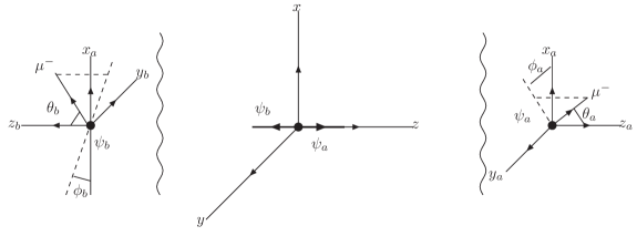
Figure 2: Definition of the $\chi_{b}\to 2(\mu^{+}\mu^{-})$ kinematics. The figure in the center corresponds to $\chi_{b}$-rest frame, left and right figures correspond to rest frames of $\psi_{b}$- and $\psi_{a}$-mesons.

$$\Gamma^{(J)}_{4} \sim \sum\limits_{\mu}\hat{\rho}_{\mu}\int d\Phi_{4}(\chi\to 2(\mu^{+}\mu^{-}))\left|\mathcal{M}^{(J)}_{\mu}\right|^{2}\sim$$ (9)

$$\sim \sum\limits_{\mu}\hat{\rho}_{\mu}\sum\limits_{\lambda_{a,b}}\sum\limits_{\bar{\lambda}_{a,b}}\int d\Omega d\Omega_{a}d\Omega_{b}d^{(J)}_{\mu\lambda}(\theta_{\chi})d^{(J)}_{\mu\bar{\lambda}}(\theta_{\chi})\times$$

$$\times \tilde{\mathcal{A}}^{(J)}_{\lambda_{a},\lambda_{b}}\tilde{\mathcal{A}}^{(J)*}_{\bar{\lambda}_{a},\bar{\lambda}_{b}}\mathcal{U}_{\lambda_{a}\bar{\lambda}_{a}}(\theta_{a},\phi_{a})\mathcal{U}_{\lambda_{b}\bar{\lambda}_{b}}(\theta_{b},\phi_{b}).$$

Here $\bar{\lambda}=\bar{\lambda}_{a}-\bar{\lambda}_{b}$, $d\Omega_{a,b}=\sin\theta_{a,b}d\theta_{a,b}d\phi_{a,b}$ are the solid angles or the decays $\psi_{a,b}\to\mu^{+}\mu^{-}$ in $\psi$-meson rest frame, and $\mathcal{U}_{\lambda\bar{\lambda}}(\theta,\phi)=\mathcal{N}_{\lambda}(\theta,\phi)\mathcal{N}^{*}_{\bar{\lambda}}(\theta,\phi)$. The functions $\mathcal{U}_{\lambda,\bar{\lambda}}(\theta,\phi)$ satisfy the relations

$$\mathcal{U}_{\lambda,\bar{\lambda}}(\theta,\phi) = \mathcal{U}^{*}_{\bar{\lambda},\lambda}(\theta,\phi)=(-1)^{\lambda-\bar{\lambda}}\mathcal{U}_{-\bar{\lambda},-\lambda}(\theta,\phi),$$

and the explicit expression are

$$\mathcal{U}_{1,1}(\theta,\phi) = m^{2}g^{2}(2-\sin^{2}\theta)=\mathcal{U}_{-1,-1}(\theta,\phi)$$

$$\mathcal{U}_{0,0}(\theta,\phi) = 2m^{2}g^{2}\sin^{2}\theta$$

$$\mathcal{U}_{1,0}(\theta,\phi) = \sqrt{2}m^{2}g^{2}\sin\theta\cos\theta e^{i\phi}=-\mathcal{U}_{0,-1}(\theta,\phi)$$

$$\mathcal{U}_{0,1}(\theta,\phi) = \sqrt{2}m^{2}g^{2}\sin\theta\cos\theta e^{-i\phi}=-\mathcal{U}_{-1,0}(\theta,\phi)$$

$$\mathcal{U}_{1,-1}(\theta,\phi) = m^{2}g^{2}\sin^{2}\theta e^{2i\phi}.$$

Here $g$ is the effective constant of the $\psi\mu^{+}\mu^{-}$ vertex, that can be expressed through the width of $\psi$ leptonic decay:

$$g^{2} = 12\pi\frac{\Gamma(\psi\to\mu^{-}\mu^{+})}{m}$$

and we have neglected the muon mass. When deriving the formula (9) we have used the factorization of the 4-particle phase space

$$d\Phi_{4}(\chi\to\psi\psi\to\mu^{+}\mu^{-}\mu^{+}\mu^{-}) \sim dp_{a}^{2}dp_{b}^{2}d\Phi_{2}(\chi\to\psi\psi)d\Phi_{2}(\psi_{a}\to\mu^{+}\mu^{-})d\Phi_{2}(\psi_{b}\to\mu^{+}\mu^{-})$$

and the relation

$$\left|\frac{1}{p_{a,b}^{2}-M_{\psi}^{2}}\right|^{2} \sim \frac{1}{\mathcal{M}_{\psi}\Gamma_{\psi}}\delta\left(p_{a,b}^{2}-M_{\psi}^{2}\right),$$

that is caused by the smallness of the $\psi$-meson total width.

IV Final muon distributions

From the formula (9) we can derive the distributions by the kinematic variables of final muons. These distributions will be considered in this section.

Let us consider the case when only one $\mu^{+}\mu^{-}$-pair is registered. In this case we can construct a normalized helicity density matrix

$$\rho_{\lambda_{a},\bar{\lambda}_{a}} = \frac{\sum\limits_{\lambda_{b}}\tilde{\mathcal{A}}^{(J)}_{\lambda_{a},\lambda_{b}}\tilde{\mathcal{A}}^{(J)*}_{\bar{\lambda}_{a},\lambda_{b}}}{\sum\limits_{\lambda_{a},b}|\tilde{\mathcal{A}}^{(J)}_{\lambda_{a},\lambda_{b}}|^{2}}.$$

The distribution by the angle $\theta_{a}$ has the form

$$\frac{1}{\Gamma}\frac{d\Gamma}{d\cos\theta_{a}} = \frac{3}{4}\left\{(1-\rho_{0,0})\cos^{2}\theta_{a}+\frac{1+\rho_{0,0}}{2}\sin^{2}\theta_{a}\right\}.$$

Using this expression one can construct the distributions by the experimentally observable variables. If $E_{\mu}$ is the energy of the final muon in the rest frame of the initial bottomonium, than the distribution by this variable has the form

$$\frac{1}{\Gamma}\frac{d\Gamma}{dE_{\mu}} = \frac{3}{2M\beta}\left\{1+\rho_{0,0}-\frac{3\rho_{0,0}-1}{\beta^{2}}\left(\frac{4E_{\mu}}{M}-1\right)^{2}\right\},$$ (10)

where $\beta=\sqrt{1-4m^{2}/M^{2}}$ is the $\psi$ velocity in the $\chi_{b}$ rest frame. It is clearly seen that the form of this distribution depends strongly on the value of the parameter $\rho_{0,0}$. If $\rho_{0,0}=1/3$ the differential width will not depend on the energy of the muon, whereas for $\rho_{0,0}>1/3$ or $\rho_{0,0}<1/3$ we will have a parabola with positive or negative main coefficient. The parameter $\rho_{0,0}$ is expressed through the reduced helicity amplitudes according to

$$\rho_{0,0} = \frac{|\tilde{\mathcal{A}}_{0,0}|^{2}+2|\tilde{\mathcal{A}}_{1,0}|^{2}}{|\tilde{\mathcal{A}}_{0,0}|^{2}+2|\tilde{\mathcal{A}}_{1,-1}|^{2}+2|\tilde{\mathcal{A}}_{1,1}|^{2}+4|\tilde{\mathcal{A}}_{1,0}|^{2}}.$$

In the second section we have mentioned that the reduced amplitudes $\mathcal{A}^{(J)}_{\lambda_{a},\lambda_{b}}$ should satisfy the restrictions $|\lambda_{a}-\lambda_{b}|\leq J$ and the chiral suppression (2) should take place. A result of these restrictions is that in the massless $\psi$ limit we have $\rho_{0,0}=1$ for scalar bottomonium and $\rho_{0,0}=1/3$ for tensor one. Since the mass of the $\psi$-meson is small compared with the mass of $\chi_{b}$, similar results should take place also for real $\psi$, so the forms of the muon energy distributions for scalar and tensor bottomonia a different. In figure 3 we show the distribution $d\Gamma/dE_{\mu}$ for scalar and tensor bottomonia (solid and dashed lines respectively) for different sets of the $\psi$-meson wave functions. It is clearly seen that from this distribution one can determine the spin of $\chi_{b}$ meson and set the restrictions on the $\psi$-meson wave function. Similar situation is observed also for the distributions by the transverse muon momentum $k_{\perp}$, that is the component of the muon momentum that is orthogonal to the momentum of the parent $\psi$-meson. From the formula (10) one can easily obtain the analytical expression for this distribution:

$$\frac{1}{\Gamma}\frac{d\Gamma}{dk_{\perp}} = \frac{3}{m}\frac{k_{\perp}}{\sqrt{m^{2}-4k_{\perp}^{2}}}\left\{1-\rho_{0,0}-(1-3\rho_{0,0})\frac{2k_{\perp}^{2}}{m_{2}}\right\}.$$

Unfortunately, the first factor masks the form of this distribution, so it is hard to distinguish the scalar bottomonium from the tensor one from it.

Figure 3: Normalized muon energy distributions in the decays $\chi_{b0}\to 2(\mu^{+}\mu^{-})$ (solid line) and $\chi_{b2}\to 2(\mu^{+}\mu^{-})$ (dashed line) for different sets of $\psi$-meson wave functions

Let us now proceed to the case when the decays of both $\psi$-mesons are registered. Here we will consider the distribution by the angle between decay planes, that is the planes formed by the final muon momenta. This angle is expressed through the azimuthal angles $\phi_{a,b}$ by the relation $\delta\phi=\phi_{a}+\phi_{b}$, and the normalized distribution over this angle have the form

$$\frac{1}{\Gamma_{4}^{(J)}}\frac{d\Gamma_{4}^{(J)}}{d\delta\phi} = \frac{1}{\pi}\left\{1+\frac{|\tilde{\mathcal{A}}^{(J)}_{1,1}|^{2}}{\sum\limits_{\lambda_{a,b}}|\tilde{\mathcal{A}}^{(J)}_{\lambda_{a},\lambda_{b}}|^{2}}\frac{\cos 2\delta\phi}{4}\right\}.$$

We show the distributions by this angle in the figure 4. It is hard to use them for separating $\chi_{b0}$ and $\chi_{b2}$-mesons, but these distributions give us the value of the matrix element $|\tilde{\mathcal{A}}^{(J)}_{1,1}|$.

Figure 4: Normalized $\delta\phi$ distributions in the decays $\chi_{b0}\to 2(\mu^{+}\mu^{-})$ (solid line) and $\chi_{b0}\to 2(\mu^{+}\mu^{-})$ (dashed line) for different sets of $\psi$-meson wave functions

V Conclusion

In the works Kartvelishvili and Likhoded (1984); Braguta et al. (2005) it was proposed to use the decays $\chi_{b0,2}\to\psi\psi$ for the registration of $\chi_{b0,2}$ mesons. Here we continue the consideration of this question and study the decays $\chi_{b0,2}\to\psi\psi\to 2(\mu^{+}\mu^{-})$.

One of the questions that arise in the observation of scalar and tensor bottomonia is the determination of the spin of this particle. Since the difference between their masses is tiny ($M_{\chi_{b2}}-M_{\chi_{b0}}\approx 50$ MeV), it could be smaller than the instrumental error of the detector. That is why it will be rather difficult to determine the spin of the meson from its mass and one needs to have some other methods for the separation of $\chi_{b0}$- and $\chi_{b2}$-mesons. In this paper we show, that this separation can be performed using the angular distributions of $\psi$-mesons produced in the reactions $\chi_{b0,2}\to\psi\psi$, or the distributions of the final muons produced in the decays $\chi_{b0,2}\to\psi\psi\to 2(\mu^{+}\mu^{-})$.

From this distributions one can also get an additional information about the wave functions of intermediate $\psi$-mesons. In this work we consider several sets of these wave functions and show that the the distributions by final muon energy in the $\chi_{b}$ rest frames for these sets differ from each other.

The author thanks A.K. Likhoded for useful discussions. This work was partially supported by Russian Foundation for Basic Research under grant no.04-02-17530, Russian Education Ministry grant no.E02-31-96, CRDF grant no.MO-011-0, Scientific School grant no.SS-1303.2003.2.

References

Brambilla et al. (2004)
N. Brambilla
et al. (2004), eprint hep-ph/0412158.
Kartvelishvili and
Likhoded (1984)
V. G. Kartvelishvili
and A. K.
Likhoded, Yad. Fiz.
40, 1273 (1984).
Braguta et al. (2005)
V. V. Braguta,
A. K. Likhoded,
and A. V.
Luchinsky, Phys. Rev.
D72, 094018
(2005), eprint hep-ph/0506009.
Haber (1994)
H. E. Haber
(1994), eprint hep-ph/9405376.
Anselmino and Murgia (1993)
M. Anselmino and
F. Murgia,
Phys. Rev. D47,
3977 (1993).
Chernyak and Zhitnitsky (1984)
V. L. Chernyak and
A. R. Zhitnitsky,
Phys. Rept. 112,
173 (1984), eprint IYF-83-103.
Chliapnikov et al. (1979)
P. V. Chliapnikov,
V. G. Kartvelishvili,
V. V. Knyazev,
and A. K.
Likhoded, Nucl. Phys.
B148, 400 (1979).
Braguta et al. (2006)
V. V. Braguta,
A. K. Likhoded,
and A. V.
Luchinsky, Phys. Rev.
D73, 034021
(2006), eprint hep-ph/0510060.
Olsson et al. (1985)
M. G. Olsson,
A. D. Martin,
and A. W.
Peacock, Phys. Rev.
D31, 81 (1985).