Quenching of Leading Jets and Particles: the $p_{\perp}$ Dependent Landau-Pomeranchuk-Migdal effect from Nonlinear $k_{\perp}$ Factorization

Abstract

We report the first derivation of radiative nuclear stopping (the Landau-Pomeranchuk-Migdal effect) for leading jets at fixed values of the transverse momentum $p$ in the beam fragmentation region of hadron-nucleus collisions from RHIC (Relativistic Heavy Ion Collider) to LHC (Large Hadron Collider). The major novelty of this work is a derivation of the missing virtual radiative pQCD correction to these processes - the real-emission radiative corrections are already available in the literature. We manifestly implement the unitarity relation, which in the simplest form requires that upon summing over the virtual and real-emission corrections the total number of scattered quarks must exactly equal unity. For the free-nucleon target, the leading jet spectrum is shown to satisfy the familiar linear Balitsky-Fadin-Kuraev-Lipatov leading log-${1\over x}$ (LL${1\over x}$) evolution. For nuclear targets, the nonlinear $k_{\perp}$-factorization for the LL-${1\over x}$ evolution of the leading jet spectrum is shown to exactly match the equally nonlinear LL${1\over x}$ evolution of the collective nuclear glue – there emerges a unique linear $k_{\perp}$-factorization relation between the two nonlinear evolving nuclear observables. We argue that within the standard dilute uncorrelated nucleonic gas treatment of heavy nuclei, in the finite energy range from RHIC to LHC, the leading jet spectrum can be evolved in the LL${1\over x}$ Balitsky-Kovchegov approximation. We comment on the extension of these results to, and their possible reggeon field theory interpretation for, mid-rapidity jets.

I Introduction

In this communication we address two related issues in the perturbative Quantum Chromo Dynamics (pQCD) description of the single-jet inclusive spectra in hadron-nucleon and hadron-nucleus collisions. Our principal interest is in the nonlinear $k_{\perp}$ factorization for the pQCD radiative quenching (stopping) of leading jets with fixed transverse momentum $p$ produced at large values of the Feynman variable $x_{F}$, i.e., in the beam fragmentation region of hadron-nucleon and hadron-nucleus collisions. As it has become customary for the nuclear dependence of radiative effects, we refer to nuclear stopping of leading jets at fixed $p$ as the $p$-dependent Landau-Pomeranchuk-Migdal (LPM) effect. There is an extensive literature on the LPM effect for mid-rapidity jets, where the prime concern is in the radiation induced loss of the transverse, with respect to the hadron-nucleus collision axis, momentum of the jet when one integrates over the transverse momentum of the radiation with respect to the jet axis (SlavaLPM , for reviews and further references see SlavaReview ; KovchegovReview ). In the mid-rapidity kinematics, the transverse momentum of radiation with respect to the parent high-$p_{\perp}$ parton only amounts to a small shift of the (pseudo)rapidity of the high-$p_{\perp}$ parton which is hardly observable due to the boost invariance in the mid-rapidity region. In contrast to that, leading jets with $x_{F}\sim 1$ are generated by hard scattering of valence quarks. The density of valence quarks drops rapidly at large values of the Bjorken variable in the beam nucleon, $x_{N}\to 1$, which entails that the $x_{F}$ dependence of the leading jet cross section is extremely sensitive to the radiative energy loss. We develop a nonlinear $k_{\perp}$ factorization description of leading jet production with full allowance for the real and virtual QCD radiative corrections. In the second part we focus on the leading log${1\over x}$ (LL${1\over x}$) properties of the leading jet spectrum. We argue that this spectrum offers a long sought linear mapping of the unintegrated collective nuclear glue and comment on the extension of this finding to mid-rapidity jets.

Within pQCD, there are several subtleties in the application of factorization theorems to the leading quark production in $qN,qA$ collisions. In the more familiar collinear approximation described in all textbooks Textbook , the relevant pQCD subprocess is hard scattering of valence quarks off soft gluons with $x\ll 1$ in the target, which can also be viewed as a hard breakup (excitation) $q\to q^{\prime}g$. All partons enter the hard pQCD scattering with vanishing transverse momentum and the large $p_{\perp}$ of the observed jet is generated in the real-emission hard breakup. The inadequacy of such a collinear approximation is well known, a recent concise discussion of the necessity of fully unintegrated parton densities with explicit allowance for transverse momenta is found in CollinsZu . In the high-energy limit, the latter is furnished by the so-called $k_{\perp}$-factorization which goes back to the classic 1975-1978 works on the Balitsky-Fadin-Kuraev-Lipatov (BFKL) equation for the small-$x$ evolution of the unintegrated glue (KLF ; BFKL , see also the recent review on $k_{\perp}$-factorization and more references in Smallx ; Antoni ). In contrast to the collinear factorization, within the $k_{\perp}$-factorization, the hard breakup $q\to q^{\prime}g$ is but the real-emission pQCD radiative correction (REC) to the lower order (Born) subprocess, which is the quasielastic scattering $qN\to qN^{*}$, $qA\to qA^{*}$, where the target debris $N^{*},A^{*}$ is left in a color excited state. Evidently, the real-emission must be complemented by the matching virtual pQCD radiative corrections (VRC) to the lower order quasielastic scattering - the real-emission and virtual radiative corrections are two integral parts of the small-$x$ evolution of quasielastic scattering, see Fig. 1.

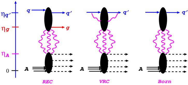
Figure 1: The real emission (REC) and virtual radiation (VRC) contributions to the Born spectrum of leading quark jets in inclusive production off nuclei. The (pseudo)rapidity of radiation correction gluons runs between the quark jet rapidity and the nuclear boundary condition rapidity $\eta_{A}=\log{1\over x_{A}}$, where $x_{A}$ is defined by Eq. (19).

Hard scattering off free nucleons is described by single-gluon exchange in the $t$-cannel. In collisions with nuclei, the enhancement of multigluon exchanges leads to a novel concept of nonlinear $k_{\perp}$ factorization Nonlinear ; PionDijet ; QuarkGluonDijet ; Nonuniversality ; GluonGluonDijet ; Paradigm . The Born and VRC amplitudes describe final states in which the large transverse momentum of the leading jet is compensated by hadrons at rapidities $\eta\mathrel{\hbox to0.0pt{\lower 4.0pt\hbox{\hskip 1.0pt$\sim$}\hss}\raise 1.0pt\hbox{$<$}}\eta_{A}$, while in REC such a compensation is provided also by gluon jets with rapidities $\eta_{A}\mathrel{\hbox to0.0pt{\lower 4.0pt\hbox{\hskip 1.0pt$\sim$}\hss}\raise 1.0pt\hbox{$<$}}\eta_{g}\mathrel{\hbox to0.0pt{\lower 4.0pt\hbox{\hskip 1.0pt$\sim$}\hss}\raise 1.0pt\hbox{$<$}}\eta_{q^{\prime}}$. A theoretical treatment of the $p$ dependent LPM effect for leading jets is necessary for the interpretation of the forthcoming experimental data on leading particles from the RHIC to LHC (BRAHMS and references therein).

The interplay of the virtual and real radiative corrections to single jet spectra is controlled by the unitarity condition. In its simplest form unitarity demands that the multiplicity of final state leading quarks from the real radiation, and from the VRC-corrected lower order (Born) quasielastic scattering add up exactly to unity. In other words, the small-$x$ evolutions of the total inclusive cross section for the leading quark production and of the total cross section of the quark-target interaction must preserve their exact equality. Evidently, the accurate evaluation of the energy loss requires the REC for a finite fraction, $z_{g}$, of the incident quark’s momentum carried by the radiated gluon. Correspondingly, the VRC must be calculated to a matching accuracy. While the required real-emission spectra do exist in the literature for both the free-nucleon and nuclear targets (we follow the approach of Ref. SingleJet , for related works and further references see Kovchegov ; Blaizot ; Baier ), the matching derivation of virtual radiative corrections was not yet available - it is a major novelty of this paper. Our derivation of the combined VRC and REC fully respects the $s$-channel unitarity constraints and paves the way to a first consistent description of the LPM effect for leading jets for fixed $p$ of the jet.

Much insight into the interplay of the virtual and real-emission radiative corrections for nuclear targets comes from the study of LL${1\over x}$ evolution of the LPM effect-deconvoluted inclusive spectra of leading particles, i.e., neglecting the radiative energy loss. At moderately high energies, the unitarity constraints in hard $qN$ collisions are still unimportant and they can be described by single-gluon exchange in the $t$-channel between the projectile and target. In this case a comparison of the LL${1\over x}$ evolution of the LPM-effect deconvoluted leading parton spectrum and of the BFKL evolution of the unintegrated glue of the nucleon leads to a simple $k_{\perp}$-factorization relationship

$${d{\sigma}_{Qel}\over d^{2}\mbox{\boldmath$p$}}={1\over 2}f(x,\mbox{\boldmath$p$})$$ (1)

(for the definition of the unintegrated glue $f(x,\mbox{\boldmath$p$})$ in the free nucleon see below). I.e., the leading quark spectrum satisfies the same BFKL small-$x$ evolution equation as the unintegrated glue KLF ; BFKL , and this spectrum emerges as a direct probe of the unintegrated glue in the target nucleon. It is remarkable that our derivation of this property makes a direct use the $s$-channel unitarity for color dipole scattering. In the realm of the BFKL approach, this property can be regarded as a straightforward consequence of the correspondence between LL${1\over x}$ approximation and the dominance of multiregge production processes KLF ; BFKL ; FadinNew .

In contrast to the single $t$-channel gluon exchange with the free-nucleon target, multiple gluon exchanges with the target nucleus are enhanced by a large thickness of the nucleus. Here the very possibility of describing a nucleus by a unique collective unintegrated glue, and the existence of factorization theorems, become problematic. Various aspects of this issue have been addressed to within the so-called Color Glass Condensate approach, in which the starting idea was to describe the nucleus by the collective Weizsäcker-Williams gluon density (CGC and references therein). More recently, much progress has been made within the nonlinear $k_{\perp}$-factorization reformulation of the multiple scattering theory for color dipoles. Within the color dipole approach, the extensive previous studies of the dijet spectra (Nonlinear ; PionDijet ; QuarkGluonDijet ; Nonuniversality ; GluonGluonDijet ; Paradigm , see also the recent Ref. Fujii ) and single-jet spectra SingleJet revealed a striking breaking of the conventional linear $k_{\perp}$ factorization for hard processes in a nuclear environment. Specifically, all the dijet observables can be represented as nonlinear quadratures of the collective nuclear glue defined in terms of a reference nuclear process - production of coherent diffractive dijets NSSdijet ; NSSdijetJETPLett . On the other hand, in Refs. Nonlinear ; SingleJet we noticed the phenomenon of Abelianization of the single particle spectra – to LL${1\over x}$ the nonlinear $k_{\perp}$-factorization simplifies down to the linear $k_{\perp}$-factorization subject to the judicious choice of the component of the color space density matrix for the collective nuclear glue. Here we demonstrate that, at least to the first order of LL${1\over x}$, a similar Abelianization takes place for the leading jet spectrum from inelastic processes.

When speaking of $k_{\perp}$-factorization for nuclear collisions, one needs to define the collective nuclear glue in terms of the properly chosen physics observable. Here we start with the BFKL definition of the unintegrated glue for free nucleons KLF ; BFKL . As noticed in NZsplit , this unintegrated glue can be directly measured in diffractive production of dijets (for other applications of the unintegrated glue see the reviews in Smallx ; Antoni ; CollinsZu ; CollinsAPP ). Generalizing this observation to nuclear targets NSSdijet ; Nonlinear , we define the collective nuclear glue in terms of the color-dipole nuclear S-matrix which is accessible experimentally via diffractive dijets. The LL${1\over x}$ evolution of the so-defined glue is a nonlinear one. The REC to the inclusive single leading parton spectrum derived in SingleJet is a nonlinear functional of the collective nuclear glue. Equally highly nonlinear is the VRC correction to quasielastic parton–nucleus scattering derived in this paper. Our nontrivial finding is that the leading parton spectrum and the collective glue share identical first iteration of the nonlinear LL${1\over x}$ evolution, which is the second novelty of our paper. One is tempted to conjecture that the spectrum of leading jets is linear $k_{\perp}$-factorizable in terms of the collective nuclear glue to all order of the nonlinear LL${1\over x}$ evolution, i.e., it is a long sought unique linear probe of the collective nuclear glue. It is by now understood that the closed form of all-order LL${1\over x}$ evolution for nuclei does not exist (a detailed review is found in Trianta ). Still we argue that in view of a high accuracy of the dilute uncorrelated nucleonic gas picture of heavy nuclei, the small-$x$ evolution of the leading jet spectrum from RHIC to LHC can to a controlled accuracy be described by several iterations of the Balitsky-Kovchegov (BK) approximation BalitskyNonlinear ; KovchegovNonlinear .

We find it very instructive to compare nonlinear $k_{\perp}$-factorization properties of the LL${1\over x}$ evolution of the inclusive spectrum of leading quarks belonging to the color-triplet (fundamental) and color-octet (adjoint) representations of $SU(N_{c})$. The latter case is of interest from the viewpoint of supersymmetric QCD, one can also think of leading gluons in interactions of glueballs. A pattern of the nonlinear $k_{\perp}$-factorization for the spectrum changes strikingly from the triplet to octet quarks, equally different is the nonlinear BFKL evolution of the components of the color density matrix for the collective glue for the triplet-antitriplet and octet-octet color dipoles. For instance, for strongly absorbing nucleus and triplet-antitriplet dipoles, the nonlinear BFKL evolution looks as a fusion of two nuclear pomerons, i.e., it is dominated by triple-pomeron interactions. In striking contrast to that, for the octet-octet dipoles the dominant term looks as a fusion of three pomerons from one component of the color density matrix for the collective nuclear glue to the fourth pomeron described by a different collective glue. In both cases, however, the evolution of the two quantities – the leading parton spectrum and the collective glue – turns out to be identical, which lends more support to our conjecture on leading jets as a linear probe of the collective nuclear glue. When reinterpreted in the reggeon field theory language, our results correspond to a full resummation of multiple pomeron exchanges enhanced by a large thickness of the target nucleus. Such a resummation is interesting on its own, an extension of these results beyond the dilute projectile and the Balitsky-Kovchegov approximations, and the challenging inclusion of the pomeron loop effects (for the review see Trianta ) go beyond the scope of the present communication.

The presentation of the main material is organized as follows. In Sec. II we introduce the basic color dipole formalism, a definition of the collective nuclear unintegrated glue and derive the differential cross section of quasielastic scattering of quarks off free nucleons and nuclei to the Born approximation. The color-dipole master formulas for the real and virtual radiative corrections to the inclusive spectrum of leading quarks are presented in Sec. III. Our derivation of the virtual correction in Sec. III.B makes a manifest use of the unitarity relation. We then proceed to the (nonlinear) $k_{\perp}$-factorization for the spectrum of leading quarks off the free nucleon (Sec. IV.A) and color-triplet quark-nucleus (Sec. IV.B) collisions as well as for the spectrum of leading color-octet quarks (and gluons) in collisions with nuclei (Sec. IV.C). These results are sufficient for the quantitative treatment of the LPM effect at fixed transverse momentum of leading jets at RHIC energies. In Sec. IV.D we revisit the issue of unitarity and demonstrate the consistency of our radiative corrections with the leading quark number sum rule. Inspired by the observations in Sec. II and Sec. IV, in Sec. V we focus on the LL${1\over x}$ evolution properties of inclusive single particle spectra, which are necessary for the extension of our technique to LHC energies. We demonstrate, that to the LL${1\over x}$ approximation, the nonlinear-evolving leading parton spectrum in parton-nucleus collisions proves to be linear $k_{\perp}$-factorizable in terms of the nonlinear-evolved collective nuclear glue. In Sec. V.D we comment on the unified description of the LL${1\over x}$ evolution of the triplet-antitriplet and octet-octet S-matrices. The subject of section V.E is a partial vindication of the BK approximation - while it is not a closed-form equation and is not really applicable to the free-nucleon target, for heavy nuclei several iterations of the BK approximation will be a useful working approximation in the range of energies from RHIC to LHC. This gives a practical procedure for the quantitative evaluations of the LPM effect for leading jets at LHC. In section V.F we comment on how our treatment of the interplay between VRC and REC extends to the production of mid-rapidity jets, and on the possible interpretation of our results from the effective reggeon field theory perspective. In the Conclusions we summarize our principal findings. In the Appendix we comment on an interesting observation that the nonlinear $k_{\perp}$-factorization component of the LL${1\over x}$ nonlinear evolution gives a pure higher twist contribution to the collective nuclear glue NonlinearBFKL .

II Leading particle spectra to the Born approximation

II.1 Leading particles from the breakup of heavy quarkonium

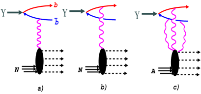
Figure 2: (a,b) The Feynman diagrams for Upsilon breakup by single-gluon exchange with the target nucleon and (c) an archetype diagram of breakup of Upsilon by a multiple-gluon exchange with the target nucleus.

To set up the framework, we start with a toy problem: the breakup of the color-singlet heavy quarkonium (let it be $\Upsilon$) in a high energy collision with the free-nucleon target $\Upsilon N\to b\bar{b}X$. Heavy quarkonium can well be approximated by its quark-antiquark Fock state with the size $R_{\Upsilon}\gg 1/m_{b}$. The lowest order pQCD subprocess is a breakup by Upsilon-gluon fusion,$\Upsilon g_{t}\to b\bar{b}$, where $g_{t}$ is the gluon exchanged in the $t$-channel. (Fig. 2). The corresponding inclusive differential cross section, obtained after summing over all excitations of the target nucleon, is well known; it is found, for instance, in PionDijet (Eqs. (4) and (5)):

$${d\sigma(\Upsilon\to b\bar{b})\over dzd^{2}\mbox{\boldmath$p$}d^{2}\mbox{\boldmath$\Delta$}}={\alpha_{S}(\mbox{\boldmath$p$}^{2})\over 2\pi N_{c}}\cdot{{\cal F}(x,\mbox{\boldmath$\Delta$}^{2})\over\Delta^{4}}$$

$$\times|\Psi_{\Upsilon}(z,\mbox{\boldmath$p$})-\Psi_{\Upsilon}(z,\mbox{\boldmath$p$}-\mbox{\boldmath$\Delta$})|^{2}.$$ (2)

Here $\alpha_{S}(\mbox{\boldmath$p$}^{2})$ is the pQCD coupling, $N_{c}$ is the number of colors, $\Psi_{\Upsilon}(z,\mbox{\boldmath$p$})$ is the lightcone wave function of the quarkonium, $p$ is the transverse momentum of the quark in the quarkonium, $z$ is the fraction of the lightcone momentum of the quarkonium carried by the quark, $\Delta$ is the total transverse momentum of the $b\bar{b}$ pair,

$${\cal F}(x,\kappa^{2})={\partial G(x,\kappa^{2})\over\partial\log\kappa^{2}}$$ (3)

is the so-called unintegrated gluon density in the target nucleon as introduced in the BFKL approach KLF ; BFKL . The Bjorken variable $x$ of the exchanged gluon equals

$$x={M_{b\bar{b}}^{2}-M_{\Upsilon}^{2}\over W_{\Upsilon p}^{2}},$$ (4)

where $W_{\Upsilon p}$ is the cms energy in the $\Upsilon p$ system and $M_{b\bar{b}}$ is the transverse mass of the excited quark-antiquark pair,

$$\quad M_{b\bar{b}}^{2}={m_{b}^{2}+\mbox{\boldmath$p$}^{2}\over z}+{m_{b}^{2}+(\mbox{\boldmath$p$}-\mbox{\boldmath$\Delta$})^{2}\over 1-z}.$$ (5)

The transverse momentum $\Delta$ of the $b\bar{b}$ pair comes entirely from the exchanged gluon and the differential cross section (2) emerges as a natural probe of the unintegrated glue ${\cal F}(x,\mbox{\boldmath$\Delta$}^{2})$. We recall that for the free nucleon target ${\cal F}(x,\kappa^{2})$ is a solution of the LL${1\over x}$ BFKL evolution equation KLF ; BFKL , a detailed discussion of the connection between the integrated glue $G(x,\kappa^{2})$ of Eq. (3) and the gluon densities of the leading order Dokshitzer-Gribov-Lipatov-Altarelli-Parisi evolution equations DGLAP is found in Refs. Kfact ; CollinsAPP ; NZglue ; INdiffglue ; Smallx and need not be repeated here.

Now consider transverse momenta $p$ much larger than the typical momentum of the Fermi motion in the quarkonium, $p_{b}\sim 1/R_{\Upsilon}$. The wave function $\Psi(z,\mbox{\boldmath$p$})$ vanishes steeply beyond $p_{b}$, and the single-quark spectrum takes the convolution form

$${d\sigma(\Upsilon\to b\bar{b})\over dzd^{2}\mbox{\boldmath$p$}}=\int d^{2}\mbox{\boldmath$\kappa$}{\alpha_{S}(\mbox{\boldmath$p$}^{2})\over 2\pi N_{c}}\cdot{{\cal F}(x,\mbox{\boldmath$\kappa$}^{2})\over\mbox{\boldmath$\kappa$}^{4}}$$

$$\times|\Psi_{\Upsilon}(z,\mbox{\boldmath$p$})-\Psi_{\Upsilon}(z,\mbox{\boldmath$p$}-\mbox{\boldmath$\kappa$})|^{2}$$

$$\approx\int d^{2}\mbox{\boldmath$\kappa$}{\alpha_{S}(\mbox{\boldmath$p$}^{2})\over 2\pi N_{c}}\cdot{{\cal F}(x,\mbox{\boldmath$\kappa$}^{2})\over\mbox{\boldmath$\kappa$}^{4}}|\Psi_{\Upsilon}(z,\mbox{\boldmath$p$}-\mbox{\boldmath$\kappa$})|^{2}$$

$$=\int d^{2}\mbox{\boldmath$\kappa$}d^{2}\mbox{\boldmath$p$}_{b}\delta(\mbox{\boldmath$p$}-\mbox{\boldmath$p$}_{b}-\mbox{\boldmath$\kappa$})$$

$$\times{dq_{b/\Upsilon}(z,\mbox{\boldmath$p$}_{b})\over d^{2}\mbox{\boldmath$p$}_{b}}\cdot{d\sigma(b\to b^{\prime})\over d^{2}\mbox{\boldmath$\kappa$}}.$$ (6)

Here

$${dq_{b/\Upsilon}(z,\mbox{\boldmath$p$}_{b})\over d^{2}\mbox{\boldmath$p$}_{b}}=|\Psi_{\Upsilon}(z,\mbox{\boldmath$p$}_{b})|^{2}$$ (7)

is the momentum distribution of quarks in the quarkonium and

$${d\sigma(b\to b^{\prime})\over d^{2}\mbox{\boldmath$\kappa$}}={\alpha_{S}(\mbox{\boldmath$p$}^{2})\over 2\pi N_{c}}\cdot{{\cal F}(x,\mbox{\boldmath$\kappa$}^{2})\over\mbox{\boldmath$\kappa$}^{4}}$$ (8)

must be interpreted as a differential cross section of the valence quark quasielastic scattering $bN\to b^{\prime}X$. Furthermore, the longitudinal momentum distribution of leading quarks is given by precisely the transverse momentum-dependent $z$-distribution in the quarkonium – $z$ is the Feynman variable of the observed quark. As such, the convolution (6) can be regarded as the archetype $k_{\perp}$-factorization for the production of hard leading quark jets in high-energy hadron-nucleon collisions. The adjective ‘hard’ refers to the jet momenta harder than the intrinsic momentum of quarks in the quarkonium: $\mbox{\boldmath$p$}^{2}\gg\langle p_{b}^{2}\rangle$. Now we proceed to the $k_{\perp}$-factorization properties of the quasielastic scattering of partons – quarks and gluons – off free nucleons and heavy nuclei.

II.2 The free-nucleon target: the dipole cross section, unintegrated glue and quasielastic $aN$ scattering

We start with the dipole cross section for the $a\bar{a}$ color dipole. It is described by two-gluon exchange in the $t$-channel (Fig. 3). The S-matrices of the $aN$ and $\bar{a}N$ interaction at impact parameter $\mbox{\boldmath$b$}_{a}(\mbox{\boldmath$b$}_{\bar{a}})$ equal, respectively Nonlinear ,

$$\textsf{S}_{a}(\mbox{\boldmath$b$}_{a}) = \openone+i\textsf{T}_{a}^{\alpha}\hat{V}_{\alpha}\chi(\mbox{\boldmath$b$}_{a})-{1\over 2}\textsf{T}_{a}^{\alpha}\textsf{T}_{a}^{\alpha}\chi^{2}(\mbox{\boldmath$b$}_{a})\,,$$

$$\textsf{S}_{a}^{\dagger}(\mbox{\boldmath$b$}_{\bar{a}}) = \openone-i\textsf{T}_{a}^{\alpha}\hat{V}_{\alpha}\chi(\mbox{\boldmath$b$}_{\bar{a}})-{1\over 2}\textsf{T}_{a}^{\alpha}\textsf{T}_{a}^{\alpha}\chi^{2}(\mbox{\boldmath$b$}_{\bar{a}}),$$

were $\textsf{T}_{a}^{\alpha}\hat{V}_{\alpha}\chi(\mbox{\boldmath$b$})$ is the eikonal operator for the $aN$ single-gluon exchange interaction. In the realm of the Standard Model QCD, quarks belong to the color-triplet (fundamental) representation of $SU(N_{c})$, but much light on the small-$x$ evolution properties of the nuclear spectra is shed by considering quarks also in the octet (adjoint) representation of $SU(N_{c})$. One can also think of leading gluons in interactions of glueballs. The expansion (LABEL:eq:2.B.1) to the considered pQCD approximation satisfies the unitarity condition

$$\textsf{S}_{a}(\mbox{\boldmath$b$}_{a})\textsf{S}_{a}^{\dagger}(\mbox{\boldmath$b$}_{a})=\openone.$$ (10)

The spin of partons is unimportant in view of the $s$-channel helicity conservation in high energy QCD. The important observation is that $\textsf{S}_{a}^{\dagger}$ equals the S-matrix for interaction of the antiparticle $\bar{a}$ SlavaPositronium ; NPZcharm . The vertex operator $\hat{V}_{\alpha}$ for excitation of the nucleon $g^{\alpha}N\to N^{*}_{\alpha}$ into a color octet state $N^{*}_{\alpha}$ is so normalized that after the application of closure over the final state excitations $N^{*}$ the vertex $g^{\alpha}g^{\beta}NN$ equals $\langle{N}|\hat{V}_{\alpha}^{\dagger}\hat{V}_{\beta}|{N}\rangle=\delta_{\alpha\beta}$. The second order terms in (LABEL:eq:2.B.1) do already use this normalization.

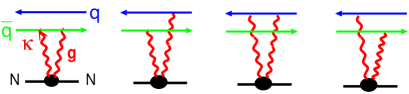
Figure 3: The four Feynman diagrams for the quark-antiquark dipole-nucleon interaction by the two-gluon pomeron exchange in the $t$-channel.

The S-matrix of the $(a\bar{a})$-nucleon interaction equals

$$\textsf{S}_{a\bar{a}}(\mbox{\boldmath$b$}_{a},\mbox{\boldmath$b$}_{\bar{a}})={\langle{N}|{\rm Tr}[\textsf{S}_{a}(\mbox{\boldmath$b$}_{a})\textsf{S}_{a}^{\dagger}(\mbox{\boldmath$b$}_{\bar{a}})]|{N}\rangle\over\langle{N}|{\rm Tr}\openone|{N}\rangle}$$

$$=1-{1\over 2}C_{a}[\chi(\mbox{\boldmath$b$}_{a})-\chi(\mbox{\boldmath$b$}_{\bar{a}})]^{2}\,.$$ (11)

where $C_{a}$ is the quadratic Casimir operator. The corresponding profile function is $\Gamma_{a\bar{a}}(\mbox{\boldmath$b$}_{a},\mbox{\boldmath$b$}_{\bar{a}})=1-\textsf{S}_{a\bar{a}}(\mbox{\boldmath$b$}_{a},\mbox{\boldmath$b$}_{\bar{a}})$, and the dipole cross section for interaction of the color-singlet $a\bar{a}$ dipole $\mbox{\boldmath$r$}=\mbox{\boldmath$b$}_{a}-\mbox{\boldmath$b$}_{\bar{a}}$ with the free nucleon is obtained upon the integration over the overall impact parameter

$$\sigma_{a\bar{a}}(x,\mbox{\boldmath$r$}) = 2\int d^{2}\mbox{\boldmath$b$}\,\Gamma_{a\bar{a}}(\mbox{\boldmath$b$},\mbox{\boldmath$b$}-\mbox{\boldmath$r$})$$ (12)

$$= C_{a}\int d^{2}\mbox{\boldmath$b$}[\chi(\mbox{\boldmath$b$})-\chi(\mbox{\boldmath$b$}-\mbox{\boldmath$r$})]^{2}$$

$$= {C_{a}\over C_{F}}\sigma(x,\mbox{\boldmath$r$})\,,$$

where $C_{F}=(N_{c}^{2}-1)/2N_{c}$ is the quark Casimir and $\sigma(x,\mbox{\boldmath$r$})$ is the dipole cross section for the $q\bar{q}$-dipole. It is related to the gluon density in the target by the $k_{\perp}$-factorization formula NZglue ; NZ94

$$\sigma(x,\mbox{\boldmath$r$}) = \int d^{2}\mbox{\boldmath$\kappa$}f(x,\mbox{\boldmath$\kappa$})[1-\exp(i\mbox{\boldmath$\kappa$}\mbox{\boldmath$r$})]\,,$$ (13)

where

$$f(x,\mbox{\boldmath$\kappa$}) = {4\pi\alpha_{S}\over N_{c}}\cdot{1\over\kappa^{4}}\cdot{\cal F}(x,\mbox{\boldmath$\kappa$}^{2}).$$ (14)

The leading Log${1\over x}$ evolution of the dipole cross section is governed by the color-dipole BFKL evolution NZ94 ; NZZBFKL , the same evolution for the unintegrated gluon density is governed by the familiar momentum-space BFKL equation KLF ; BFKL . For very large dipoles

$$\sigma_{a\bar{a},0}(x) = C_{a}\int d^{2}\mbox{\boldmath$b$}[\chi^{2}(\mbox{\boldmath$b$})+\chi^{2}(\mbox{\boldmath$b$}-\mbox{\boldmath$r$})]$$ (15)

$$= {C_{a}\over C_{F}}\int d^{2}\mbox{\boldmath$\kappa$}f(x,\mbox{\boldmath$\kappa$})$$

$$= 2C_{a}\int d^{2}\mbox{\boldmath$b$}{\langle{N}|{\rm Tr}\{\openone-\textsf{S}_{a}(\mbox{\boldmath$b$})\}|{N}\rangle\over\langle{N}|{\rm Tr}\openone|{N}\rangle}$$

$$= 2\sigma_{a}(x)={C_{a}\over C_{F}}\sigma_{0}(x),$$

where $\sigma_{0}(x)$ is the cross section for large $q\bar{q}$ dipoles.

Now we turn to the master formula for the inclusive differential cross section of quasielastic scattering $aN\to a^{\prime}N^{*}$. Only the final states $N^{*}\neq N$ are excited by the $t$-channel gluon exchange and

$${d{\sigma}_{Qel}\over d^{2}\mbox{\boldmath$p$}} = {1\over(2\pi)^{2}}\int d^{2}\mbox{\boldmath$b$}d^{2}\mbox{\boldmath$b$}^{\prime}\exp[-i\mbox{\boldmath$p$}(\mbox{\boldmath$b$}-\mbox{\boldmath$b$}^{\prime})]\sum_{N^{*}\neq N}{\langle{N}|{\rm Tr}\Big{\{}[\openone-\textsf{S}_{a}(\mbox{\boldmath$b$})]|{N^{*}}\rangle\langle{N^{*}}|[\openone-\textsf{S}_{a}^{\dagger}(\mbox{\boldmath$b$}^{\prime})]\Big{\}}|{N}\rangle\over\langle{N}|{\rm Tr}\openone|{N}\rangle}.$$

After the application of closure

$$\sum_{N^{*}\neq N}|{N^{*}}\rangle\langle{N^{*}}|+|{N}\rangle\langle{N}|=1,$$ (17)

and upon simple algebra one finds

$${d{\sigma}_{Qel}(x)\over d^{2}\mbox{\boldmath$p$}} = {1\over 2(2\pi)^{2}}\int d^{2}\mbox{\boldmath$c$}\exp[-i\mbox{\boldmath$p$}\mbox{\boldmath$c$}]$$ (18)

$$\times [\sigma_{a\bar{a},0}(x)-\sigma_{a\bar{a}}(x,\mbox{\boldmath$c$})]$$

$$= {C_{a}\over 2C_{F}}f(x,\mbox{\boldmath$p$}),$$

where $p$ is the transverse momentum of the scattered quark, cf. with Eq. (8). To this Born approximation, quasielastic scattering off the nucleon exhausts the total cross section, the pure elastic cross section is of higher order in pQCD perturbation theory - it starts with four gluons in the $t$-channel. Quasielastic $qN$ scattering emerges as a direct probe of the unintegrated gluon structure function of the target nucleon – we shall show this to hold beyond the Born approximation. The above explicit calculation of the emerging single-nucleon matrix elements is straightforward and hereafter, unless that might cause a confusion, it will be suppressed.

II.3 Quasielastic $qA$ scattering and collective nuclear glue

Here we need to specify the boundary condition of the small-x evolution. In the interaction with heavy nuclei the coherent nuclear effects evolve, and the concept of the collective unintegrated nuclear glue becomes applicable, for partons with

$$x\mathrel{\hbox to0.0pt{\lower 4.0pt\hbox{\hskip 1.0pt$\sim$}\hss}\raise 1.0pt\hbox{$<$}}x_{A}={1\over 2R_{A}m_{N}}.$$ (19)

In the Breit frame, this coherence condition corresponds to the spatial overlap and fusion of partons belonging to different nucleons at the same impact parameter in the Lorentz-contracted ultrarelativistic nucleus NZfusion . At $x\mathrel{\hbox to0.0pt{\lower 4.0pt\hbox{\hskip 1.0pt$\sim$}\hss}\raise 1.0pt\hbox{$>$}}x_{A}$ coherent nuclear effects are absent and the impulse approximation holds. The small-$x$ evolution down to $x_{A}$, the span of which could be substantial for the parametrically small $x_{A}$ for very heavy nuclei, must be performed at the free nucleon level. The evaluation of coherent nuclear effects at $x<x_{A}$ must start with the boundary conditions set by the free-nucleon quantities evaluated at $x_{0}=x_{A}$. We refer to this boundary condition as the nuclear Born approximation.

Interaction of the generic $n$-parton system with the target nucleon is described by the coupled-channel cross section operator $\hat{\Sigma}^{(n)}$. In the regime of coherent interaction with the heavy nucleus, $x\mathrel{\hbox to0.0pt{\lower 4.0pt\hbox{\hskip 1.0pt$\sim$}\hss}\raise 1.0pt\hbox{$<$}}x_{A}$, the corresponding S-matrix operator is given by the Glauber-Gribov formula Glauber ; Gribov

$$\textsf{S}[\mbox{\boldmath$b$},\hat{\Sigma}^{(n)}]=\exp[-{1\over 2}\hat{\Sigma}^{(n)}T(\mbox{\boldmath$b$})]\,,$$ (20)

where

$$T(\mbox{\boldmath$b$})=\displaystyle\int_{-\infty}^{\infty}dr_{z}\,n_{A}(\mbox{\boldmath$b$},r_{z})$$ (21)

is the optical thickness of the nucleus. The nuclear density $n_{A}(\mbox{\boldmath$b$},r_{z})$ is normalized according to $\displaystyle\int d^{3}\vec{r}\,n_{A}(\mbox{\boldmath$b$},r_{z})=\int d^{2}\mbox{\boldmath$b$}\,T(\mbox{\boldmath$b$})=A$, where $A$ is the nuclear mass number. The principal assumption behind (20) is that the nucleus is a dilute uncorrelated gas of color-singlet nucleons. Also, color dipoles are much smaller than the size of the nucleus. All the nuclear cross sections are defined per unit area in the impact parameter space.

For the transformation from the color-dipole to the momentum representation, we define the collective nuclear unintegrated gluon density per unit area in the impact parameter plane, $\phi(\mbox{\boldmath$b$},x_{0},\mbox{\boldmath$\kappa$})$, in terms of the Born-approximation nuclear profile function for the triplet-antitriplet $q\bar{q}$ dipole NSSdijet ; NSSdijetJETPLett ; Nonlinear ; NonlinearJETPLett :

$$\Gamma[\mbox{\boldmath$b$},\sigma(x_{0},\mbox{\boldmath$r$})] = 1-{\textsf{S}}[\mbox{\boldmath$b$};\sigma(x_{0},\mbox{\boldmath$r$})]$$

$$= 1-\exp\left[-{1\over 2}\sigma(x_{0},\mbox{\boldmath$r$})T(\mbox{\boldmath$b$})\right]$$

$$\equiv \int d^{2}\mbox{\boldmath$\kappa$}\phi(\mbox{\boldmath$b$},x_{0},\mbox{\boldmath$\kappa$})\Big{[}1-\exp(i\mbox{\boldmath$\kappa$}\mbox{\boldmath$r$})\Big{]}\,.$$

The expansion for $\phi(\mbox{\boldmath$b$},x_{0},\mbox{\boldmath$\kappa$})$ in terms of the collective glue for overlapping nucleons in the Lorentz-contracted ultrarelativistic nucleus, and its nuclear shadowing and antishadowing properties, are found in Nonlinear ; SingleJet . The utility of $\phi(\mbox{\boldmath$b$},x_{0},\mbox{\boldmath$\kappa$})$ stems from the observation that the driving term of small-$x$ nuclear structure functions, the amplitude of coherent diffractive production of dijets off nuclei and the single-quark spectrum from the $\gamma^{*}\to q\bar{q}$ excitation off a nucleus all take the familiar linear $k_{\perp}$-factorization form in terms of $\phi(\mbox{\boldmath$b$},x_{0},\mbox{\boldmath$\kappa$})$. Still more convenient, and more universal, would be a definition in terms of the color-dipole S matrix,

$$\Phi(\mbox{\boldmath$b$},x_{0},\mbox{\boldmath$\kappa$}) = \int{d^{2}\mbox{\boldmath$r$}\over(2\pi)^{2}}\textsf{S}[\mbox{\boldmath$b$},\sigma(x_{0},\mbox{\boldmath$r$})]\exp(-i\mbox{\boldmath$\kappa$}\cdot\mbox{\boldmath$r$})$$

$$= \textsf{S}[\mbox{\boldmath$b$},\sigma_{0}(x_{0})]\delta^{(2)}(\mbox{\boldmath$\kappa$})+\phi(\mbox{\boldmath$b$},x_{0},\mbox{\boldmath$\kappa$}),$$

which by its definition satisfies the sum rule

$$\int d^{2}\mbox{\boldmath$\kappa$}\Phi(\mbox{\boldmath$b$},x_{0},\mbox{\boldmath$\kappa$})=1.$$ (24)

Now we proceed to the differential cross section of quasielastic scattering $aA\to aA^{*}$. Heavy nuclei are strongly absorbing targets and the optical nuclear thickness $T(\mbox{\boldmath$b$})$ is a new large parameter in the problem. Because of enhanced multiple $t$-channel gluon exchanges the pure elastic scattering is no longer suppressed and final states $A^{*}$ include the ground state of the nucleus. The calculation of the total $p$ spectrum of quarks in $qA$ scattering proceeds as follows. The master formula is

$${d{\sigma}_{el+Qel}^{B}\over d^{2}\mbox{\boldmath$p$}d^{2}\mbox{\boldmath$b$}} = {1\over(2\pi)^{2}}\int d^{2}\mbox{\boldmath$c$}\exp(-i\mbox{\boldmath$p$}\cdot\mbox{\boldmath$c$})\sum_{A^{*}}{\langle{A}|{\rm Tr}\Big{\{}[\openone-\textsf{S}_{a}(\mbox{\boldmath$b$})]|{A^{*}}\rangle\langle{A^{*}}|[\openone-\textsf{S}_{a}^{\dagger}(\mbox{\boldmath$b$}-\mbox{\boldmath$c$})]\Big{\}}|{A}\rangle\over\langle{A}|{\rm Tr}\openone|{A}\rangle}.$$

(25)

The nuclear S-matrix is a product of the free-nucleon S-matrices. The technique of the calculation of nuclear matrix elements in the standard picture of a nucleus as a dilute uncorrelated gas of color-singlet nucleons is found in Glauber ; Nonlinear and need not be repeated here. We simply cite the results,

$${\langle{A}|{\rm Tr}\{\textsf{S}_{a}(\mbox{\boldmath$b$})\}|{A}\rangle\over\langle{A}|{\rm Tr}\openone|{A}\rangle}=\textsf{S}[\mbox{\boldmath$b$},\sigma_{a}(x_{0})],$$

$${\langle{A}|{\rm Tr}\{\textsf{S}_{a}(\mbox{\boldmath$b$})\textsf{S}_{a}^{\dagger}(\mbox{\boldmath$b$}-\mbox{\boldmath$c$})\}|{A}\rangle\over\langle{A}|{\rm Tr}\openone|{A}\rangle}=\textsf{S}[\mbox{\boldmath$b$},\sigma_{a\bar{a}}(x_{0},\mbox{\boldmath$c$})].$$

(26)

Now we apply (LABEL:eq:2.C.5) and notice that

$$\textsf{S}[\mbox{\boldmath$b$},\sigma_{a\bar{a},0}(x_{0})]=\textsf{S}^{2}[\mbox{\boldmath$b$},\sigma_{a}(x_{0})],$$ (27)

which leads to

$${d{\sigma}_{el+Qel}^{B}(x_{0})\over d^{2}\mbox{\boldmath$p$}d^{2}\mbox{\boldmath$b$}}=\{1-\textsf{S}[\mbox{\boldmath$b$},\sigma_{a}(x_{0})]\}^{2}\delta^{(2)}(\mbox{\boldmath$p$})$$

$$+\phi_{a\bar{a}}(\mbox{\boldmath$b$},x_{0},\mbox{\boldmath$p$}).$$ (28)

The first term describes the elastic scattering, here the delta-function $\delta^{(2)}(\mbox{\boldmath$p$})$ is a simple working approximation to the nuclear diffraction peak. The second term in the $p$ spectrum (28) describes the Born (B) approximation for the inclusive quasielastic scattering $aA\to aX$,

$${d{\sigma}_{Qel}^{B}(x_{0})\over d^{2}\mbox{\boldmath$p$}d^{2}\mbox{\boldmath$b$}}=\phi_{a\bar{a}}(\mbox{\boldmath$b$},x_{0},\mbox{\boldmath$p$}),$$ (29)

where $\phi_{a\bar{a}}(\mbox{\boldmath$b$},x_{0},\mbox{\boldmath$p$})$ is defined in terms of

$$\textsf{S}[\mbox{\boldmath$b$},\sigma_{a\bar{a}}(x_{0},\mbox{\boldmath$r$})]=\textsf{S}[\mbox{\boldmath$b$},{C_{a}\over C_{F}}\sigma(x_{0},\mbox{\boldmath$r$})].$$ (30)

Note, that the color representation dependence of the dipole cross section (12) entails a variety of the so-defined collective nuclear glue $\Phi_{a\bar{a}}(\mbox{\boldmath$b$},x_{0},\mbox{\boldmath$\kappa$})$ – the nuclear glue is a density matrix in color space. The major point is that to the considered Born approximation quasielastic scattering is linear $k_{\perp}$-factorizable in terms of the collective glue $\phi_{a\bar{a}}(\mbox{\boldmath$b$},x_{0},\mbox{\boldmath$p$})$.

Upon the integration of nuclear Born cross sections over all transverse momenta

$$\sigma_{el} = \int d^{2}\mbox{\boldmath$b$}\{1-\textsf{S}[\mbox{\boldmath$b$},\sigma_{a}(x_{0})]\}^{2},$$

$$\sigma_{in} = \sigma_{Qel}=\int d^{2}\mbox{\boldmath$b$}\{1-\textsf{S}^{2}[\mbox{\boldmath$b$},\sigma_{a}(x_{0})]\},$$ (31)

$$\sigma_{tot} = \sigma_{el}+\sigma_{in}=2\int d^{2}\mbox{\boldmath$b$}\{1-\textsf{S}[\mbox{\boldmath$b$},\sigma_{a}(x_{0})]\},$$

which are the standard Glauber formulas for the the projectile with $\sigma_{tot}^{aN}=\sigma_{a}(x_{0})$ Glauber .

III Master formulas for the real and virtual radiative corrections to inclusive single leading jet production

III.1 Real production $a\to ag$

The leading order pQCD radiative correction to the spectrum of leading particles in $aN(A)$ scattering, $a=q,g$, comes from the radiation of gluons, $aN(A)\to agN^{*}(A^{*})$. To the lowest order in pQCD, the generic partonic subprocess is $ag_{t}\to bc$. From the laboratory frame standpoint, it can be viewed as an excitation of the perturbative $|bc\rangle$ Fock state of the physical projectile $|a\rangle$ by one-gluon exchange with the target nucleon. In the case of a nuclear target one has to deal with multiple gluon exchanges which are enhanced by a large thickness of the target nucleus. Here the frozen impact parameter approximation holds, if the coherence length $l_{c}$ is larger than the diameter of the nucleus $2R_{A}$,

$$l_{c}={2E_{a}\over(Q^{*})^{2}+M_{\perp}^{2}}={1\over xm_{N}}>2R_{A}\,,$$ (33)

where

$$M_{\perp}^{2}={\mbox{\boldmath$p$}_{b}^{2}+m_{b}^{2}\over z_{b}}+{\mbox{\boldmath$p$}_{c}^{2}+m_{c}\over z_{c}}$$ (34)

is the transverse mass squared of the $bc$ state, $\mbox{\boldmath$p$}_{b,c}$ and $z_{b,c}$ are the transverse momenta and fractions of the the incident parton’s momentum carried by the outgoing partons ($z_{b}+z_{c}=1$). Notice an equivalence between the coherency condition (33) and the parton fusion condition (19). The virtuality of the incident parton $a$ equals $(Q^{*})^{2}=\mbox{\boldmath$k$}_{a}^{2}$, where $\mbox{\boldmath$k$}_{a}$ is the transverse momentum of the parton $a$ in the incident proton.

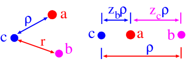
Figure 4: The color dipole structure (lhs) of the generic 3-parton state and (rhs) of the 3-parton state entering the color-dipole description of fragmentation $a\to bc$ with formation of the $bc$ dipole of size $\rho$.

The target frame rapidity structure of the considered $a\to bc$ excitation is shown in fig. 1. The beam parton has a rapidity $\eta_{a}\mathrel{\hbox to0.0pt{\lower 4.0pt\hbox{\hskip 1.0pt$\sim$}\hss}\raise 1.0pt\hbox{$>$}}\eta_{A}=\log{1/x_{A}}$, the final state partons too have rapidities $\eta_{b,c}\mathrel{\hbox to0.0pt{\lower 4.0pt\hbox{\hskip 1.0pt$\sim$}\hss}\raise 1.0pt\hbox{$>$}}\eta_{A}$. In this paper we focus on the lowest order radiative corrections without production of more secondary partons in the rapidity span between $\eta_{a}$ ($\eta_{q^{\prime}}$) and $\eta_{c}$ ($\eta_{g}$).

To the lowest order in the perturbative transition $a\to bc$ the Fock state expansion for the physical state $|a_{phys}\rangle$ reads

$$|{a_{phys}}\rangle=\sqrt{Z_{a}}|{a}\rangle_{0}+\Psi(z_{b},\mbox{\boldmath$\rho$})|{bc}\rangle_{0}$$ (35)

where $\Psi(z_{b},\mbox{\boldmath$\rho$})$ is the probability amplitude to find the $bc$ system with the separation $\rho$ in the two-dimensional impact parameter space, the subscript $"0"$ refers to bare partons. The explicit dependence of the wave functions on the virtuality $(Q^{*})^{2}$ and their relation to the parton splitting functions is found in SingleJet . Here $Z_{a}$ is the wave function renormalization, the perturbative coupling of the $a\to bc$ transition is reabsorbed into the lightcone wave function $\Psi(z_{b},\mbox{\boldmath$\rho$})$. The normalization (completeness) condition reads

$$1=Z_{a}+\int|\Psi(z_{b},\mbox{\boldmath$\rho$})|^{2}\,d^{2}\mbox{\boldmath$\rho$}dz_{b}$$ (36)

If $\mbox{\boldmath$b$}_{a}=\mbox{\boldmath$b$}$ is the impact parameter of the projectile $a$, then

$$\mbox{\boldmath$b$}_{b}=\mbox{\boldmath$b$}+z_{c}\mbox{\boldmath$\rho$},\quad\quad\mbox{\boldmath$b$}_{c}=\mbox{\boldmath$b$}-z_{b}\mbox{\boldmath$\rho$}\,,$$ (37)

see Fig. 4. Below we cite all the spectra in the $a$-target collision frame. We shall speak of the produced parton $b$ - or jet originating from this parton - as the leading one if it carries a large fraction of the beam lightcone momentum, $z_{b}\sim 1$. The Feynman variable $x_{F}$ spectra in $pN,pA$ collisions are obtained from the $z_{b}$ spectra in $qN,qA$ collisions by an obvious $k_{\perp}$-factorization convolution with the beam quark densities, see below Eq. (62).

By the conservation of impact parameters, the action of the $S$-matrix on $|{a_{phys}}\rangle$ takes a simple form

$$\textsf{S}|{a_{phys}}\rangle = S_{a}(\mbox{\boldmath$b$})\sqrt{Z_{a}}|{a}\rangle_{0}$$

$$+ S_{b}(\mbox{\boldmath$b$}_{b})S_{c}(\mbox{\boldmath$b$}_{c})\Psi(z_{b},\mbox{\boldmath$\rho$})|{bc}\rangle_{0}$$

$$= S_{a}(\mbox{\boldmath$b$})|{a_{phys}}\rangle$$

$$+ [S_{b}(\mbox{\boldmath$b$}_{b})S_{c}(\mbox{\boldmath$b$}_{c})-S_{a}(\mbox{\boldmath$b$})]\Psi(z_{b},\mbox{\boldmath$\rho$})|{bc}\rangle.$$

In the last line we explicitly decomposed the final state into the elastically scattered $|{a_{phys}}\rangle$ and the excited state $|{bc}\rangle_{0}$. The two terms in the latter describe a scattering on the target of the $bc$ system formed way in front of the target and the transition $a\to bc$ after the interaction of the state $|{a}\rangle_{0}$ with the target, as illustrated in Fig. 5. The contribution from transitions $a\to bc$ inside the target nucleus vanishes in the high-energy limit of $x\mathrel{\hbox to0.0pt{\lower 4.0pt\hbox{\hskip 1.0pt$\sim$}\hss}\raise 1.0pt\hbox{$<$}}x_{A}$.

The probability amplitude for the two-parton spectrum is given by the Fourier transform

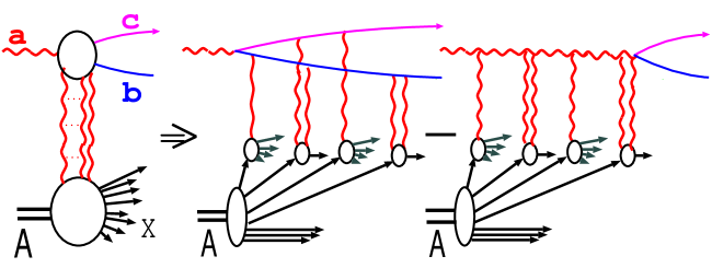
Figure 5: Typical contribution to the excitation amplitude for $aA\to bcX$, with multiple color excitations of the nucleus. The amplitude receives contributions from processes that involve interactions with the nucleus after and before the virtual decay $a\to bc$ which interfere destructively.

$$\int d^{2}\mbox{\boldmath$b$}_{b}d^{2}\mbox{\boldmath$b$}_{c}\exp[-i(\mbox{\boldmath$p$}_{b}\mbox{\boldmath$b$}_{b}+\mbox{\boldmath$p$}_{c}\mbox{\boldmath$b$}_{c})][\textsf{S}_{b}(\mbox{\boldmath$b$}_{b})\textsf{S}_{c}(\mbox{\boldmath$b$}_{c})-\textsf{S}_{a}(\mbox{\boldmath$b$})]\Psi(z_{b},\mbox{\boldmath$\rho$}).$$ (39)

The differential cross section is proportional to the modulus squared of (39)

$${d\sigma(a^{*}\to b(\mbox{\boldmath$p$}_{b})c(\mbox{\boldmath$p$}_{c}))\over dzd^{2}\mbox{\boldmath$p$}_{b}d^{2}\mbox{\boldmath$p$}_{c}}={1\over(2\pi)^{4}}\int d^{2}\mbox{\boldmath$b$}_{b}d^{2}\mbox{\boldmath$b$}_{c}d^{2}\mbox{\boldmath$b$}^{\prime}_{b}d^{2}\mbox{\boldmath$b$}^{\prime}_{c}\exp[i\mbox{\boldmath$p$}_{b}(\mbox{\boldmath$b$}_{b}-\mbox{\boldmath$b$}^{\prime}_{b})+i\mbox{\boldmath$p$}_{c}(\mbox{\boldmath$b$}_{c}-\mbox{\boldmath$b$}_{c}^{\prime})]$$

$$\times\Psi_{bc}(z_{b},\mbox{\boldmath$b$}_{b}-\mbox{\boldmath$b$}_{c})\Psi^{*}_{bc}(z_{b},\mbox{\boldmath$b$}^{\prime}_{b}-\mbox{\boldmath$b$}^{\prime}_{c})\Big{\{}\textsf{S}^{(4)}_{\bar{b}\bar{c}cb}(\mbox{\boldmath$b$}_{b}^{\prime},\mbox{\boldmath$b$}_{c}^{\prime},\mbox{\boldmath$b$}_{b},\mbox{\boldmath$b$}_{c})+\textsf{S}^{(2)}_{\bar{a}a}(\mbox{\boldmath$b$}^{\prime},\mbox{\boldmath$b$})-\textsf{S}^{(3)}_{\bar{b}\bar{c}a}(\mbox{\boldmath$b$},\mbox{\boldmath$b$}_{b}^{\prime},\mbox{\boldmath$b$}_{c}^{\prime})-\textsf{S}^{(3)}_{\bar{a}bc}(\mbox{\boldmath$b$}^{\prime},\mbox{\boldmath$b$}_{b},\mbox{\boldmath$b$}_{c})\Big{\}}.$$

(40)

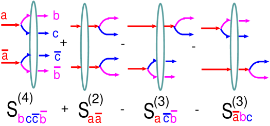
Figure 6: The S-matrix structure of the two-body density matrix for excitation $a\to bc$.

where, see Fig. 6 for an illustration,

$$\textsf{S}^{(2)}_{\bar{a}a}(\mbox{\boldmath$b$}^{\prime},\mbox{\boldmath$b$}) = \textsf{S}_{a}^{\dagger}(\mbox{\boldmath$b$}^{\prime})\textsf{S}_{a}(\mbox{\boldmath$b$}),$$

$$\textsf{S}^{(3)}_{\bar{a}bc}(\mbox{\boldmath$b$}^{\prime},\mbox{\boldmath$b$}_{b},\mbox{\boldmath$b$}_{c}) = \textsf{S}_{a}^{\dagger}(\mbox{\boldmath$b$}^{\prime})\textsf{S}_{b}(\mbox{\boldmath$b$}_{b})\textsf{S}_{c}(\mbox{\boldmath$b$}_{c}),$$

$$\textsf{S}^{(3)}_{\bar{b}\bar{c}a}(\mbox{\boldmath$b$},\mbox{\boldmath$b$}_{b}^{\prime},\mbox{\boldmath$b$}_{c}^{\prime}) = \textsf{S}_{b}^{\dagger}(\mbox{\boldmath$b$}_{b}^{\prime})\textsf{S}_{c}^{\dagger}(\mbox{\boldmath$b$}_{c}^{\prime})\textsf{S}_{a}(\mbox{\boldmath$b$}),$$

$$\textsf{S}^{(4)}_{\bar{b}\bar{c}cb}(\mbox{\boldmath$b$}_{b}^{\prime},\mbox{\boldmath$b$}_{c}^{\prime},\mbox{\boldmath$b$}_{b},\mbox{\boldmath$b$}_{c}) = \textsf{S}_{b}^{\dagger}(\mbox{\boldmath$b$}_{b}^{\prime})\textsf{S}_{c}^{\dagger}(\mbox{\boldmath$b$}_{c}^{\prime})\textsf{S}_{c}(\mbox{\boldmath$b$}_{c})\textsf{S}_{b}(\mbox{\boldmath$b$}_{b})\,.$$

Here the proper averaging over polarizations and color states of the initial parton and the summation over polarizations and color states of final state partons are understood. Next we approximate the heavy nucleus by a dilute gas of colorless nucleons and follow Glauber’s technique of summing over the final states of the target nucleus applying the closure relation Glauber . Then the nuclear matrix element of products of single-parton S-matrices would boil down to the Glauber-Gribov formula (20): $\langle{A}|\textsf{S}^{(n)}|{A}\rangle=\textsf{S}[\mbox{\boldmath$b$};\hat{\Sigma}^{(n)}]$, where $\hat{\Sigma}^{(n)}$ is the relevant $n$-parton cross section operator, for the details see Refs. Nonlinear ; QuarkGluonDijet ; GluonGluonDijet . All the multiparton states – $\bar{a}a$, $\bar{a}bc$, $\bar{b}\bar{c}a$, $\bar{b}\bar{c}cb$ – are in an overall color-singlet state and the excitation cross sections are infrared-finite despite the nonvanishing net color charge of the projectile parton $a$ NPZcharm ; SingleJet .

Integration over the transverse momentum $\mbox{\boldmath$p$}_{c}$ of the jet $c$ gives

$$\mbox{\boldmath$b$}_{c} = \mbox{\boldmath$b$}_{c}^{\prime}\,,\quad\mbox{\boldmath$b$}-\mbox{\boldmath$b$}^{\prime}=z_{b}(\mbox{\boldmath$\rho$}-\mbox{\boldmath$\rho$}^{\prime})\,,$$

$$\quad\mbox{\boldmath$b$}_{b}-\mbox{\boldmath$b$}_{b}^{\prime} = \mbox{\boldmath$\rho$}-\mbox{\boldmath$\rho$}^{\prime}\,,\quad\mbox{\boldmath$b$}^{\prime}-\mbox{\boldmath$b$}_{c}=z_{b}\mbox{\boldmath$\rho$}^{\prime}\,.$$ (42)

Then the unitarity relation

$$S_{c}^{\dagger}(\mbox{\boldmath$b$}_{c})S_{c}(\mbox{\boldmath$b$}_{c})=1$$ (43)

leads to a fundamental simplification:

$$S^{(4)}_{\bar{b}\bar{c}cb}(\mbox{\boldmath$b$}_{b}^{\prime},\mbox{\boldmath$b$}_{c}^{\prime},\mbox{\boldmath$b$}_{b},\mbox{\boldmath$b$}_{c}) = S_{b}^{\dagger}(\mbox{\boldmath$b$}_{b}^{\prime})S_{c}^{\dagger}(\mbox{\boldmath$b$}_{c})S_{c}(\mbox{\boldmath$b$}_{c})S_{b}(\mbox{\boldmath$b$}_{b})$$ (44)

$$= S_{b}^{\dagger}(\mbox{\boldmath$b$}_{b}^{\prime})S_{b}(\mbox{\boldmath$b$}_{b})$$

$$= S^{(2)}_{\bar{b}b}(\mbox{\boldmath$b$}_{b}^{\prime},\mbox{\boldmath$b$}_{b})\ ,$$

i.e., the effect of interactions of the spectator parton $c$ vanishes upon the summation over all its color states and integration over all its transverse momenta (NPZcharm , see also a discussion in SingleJet ) the only trace of the observed parton $b$ having been produced in the fragmentation $a\to bc$ is in the density matrix $\Psi(z_{b},\mbox{\boldmath$b$}_{b}-\mbox{\boldmath$b$}_{c})\Psi^{*}(z_{b},\mbox{\boldmath$b$}^{\prime}_{b}-\mbox{\boldmath$b$}^{\prime}_{c})$ which defines the transverse momentum distribution of the parton $b$ in the beam parton $a$ and the partition $z_{b}\,,\,z_{c}=(1-z_{b})$, of the longitudinal momentum between the final state partons. The applications of the master formula (40) to the calculation of the real emission spectra for the free-nucleon and nuclear targets are found in SingleJet .

III.2 Derivation of the virtual radiative correction from the unitarity relation

The relevance of the unitarity has already been explained in the Introduction. It is especially obvious in $qN(A)$ scattering. The opening of the new channel $q\to qg$ renormalizes, via unitarity, the Born cross section of the lower order quasielastic scattering $qN(A)\to q^{\prime}N^{*}(A^{*})$. The VRC is precisely that unitarity driven renormalization. The real emission and the virtual correction must so conspire, that the total multiplicity of leading quarks in the final state is exactly unity. We show here two derivations which have already been used in the related works NPZcharm ; NZ94 ; NZZBFKL .

The first approach is a direct perturbative solution of the unitarity relation (NPZcharm , for an extensive use in the theory of the LPM effect see SlavaLPM ). We define the radiatively corrected S-matrix of elastic scattering,

$$\textsf{S}_{el}(\mbox{\boldmath$b$},x)=\textsf{S}_{a}(\mbox{\boldmath$b$},x_{0})+\delta\textsf{S}_{a}(\mbox{\boldmath$b$},x),$$ (45)

and the excitation (real emission) operator

$$\textsf{S}_{ex}(\mbox{\boldmath$b$},x)=\textsf{S}_{b}(\mbox{\boldmath$b$}_{b},x_{0})\textsf{S}_{c}(\mbox{\boldmath$b$}_{c},x_{0})-\textsf{S}_{a}(\mbox{\boldmath$b$},x_{0}).\\$$

Then the unitarity relation would read

$$\textsf{S}(\mbox{\boldmath$b$},x)\textsf{S}^{\dagger}(\mbox{\boldmath$b$},x)=\textsf{S}_{el}(\mbox{\boldmath$b$},x)\textsf{S}_{el}^{\dagger}(\mbox{\boldmath$b$},x)$$

$$+\int{\cal D}_{bc}\Psi^{*}_{bc}\Psi_{bc}\textsf{S}_{ex}(\mbox{\boldmath$b$},x)\textsf{S}_{ex}^{\dagger}(\mbox{\boldmath$b$},x)=1,$$ (46)

where we explicitly separated the contributions from the elastic and real emission channels, ${\cal D}_{bc}$ is the short hand notation for the integral over the $bc$ dipole parameters, ${\cal D}_{bc}=d^{2}\mbox{\boldmath$\rho$}dz_{c}$. If the boundary condition for the small-$x$ evolution is defined at $x_{0}$, then the integration over $dz_{c}$ extends over the interval $[x/x_{0},1]$. We recall that $\Psi^{*}_{bc}\Psi_{bc}\propto\alpha_{S}$ and the real emission contribution to (46) must be regarded as the pQCD perturbation. Making use of the explicit form of $\textsf{S}_{ex}(\mbox{\boldmath$b$},x)$, to the linear order in $\delta\textsf{S}_{a}(\mbox{\boldmath$b$},x)$ we find

$$\delta\textsf{S}_{a}(\mbox{\boldmath$b$},x)\textsf{S}_{a}^{\dagger}(\mbox{\boldmath$b$},x_{0})+\textsf{S}_{a}(\mbox{\boldmath$b$},x_{0})\delta\textsf{S}_{a}^{\dagger}(\mbox{\boldmath$b$},x) = \int{\cal D}_{bc}\Psi^{*}_{bc}\Psi_{bc}[\textsf{S}_{b}(\mbox{\boldmath$b$}_{b},x_{0})\textsf{S}_{c}(\mbox{\boldmath$b$}_{c},x_{0})\textsf{S}_{a}^{\dagger}(\mbox{\boldmath$b$},x_{0})-1]$$ (47)

$$+ \int{\cal D}_{bc}\Psi^{*}_{bc}\Psi_{bc}[\textsf{S}_{a}(\mbox{\boldmath$b$}_{a},x_{0})\textsf{S}_{c}^{\dagger}(\mbox{\boldmath$b$}_{c},x_{0})\textsf{S}_{b}^{\dagger}(\mbox{\boldmath$b$}_{b},x_{0})-1].$$

Evidently, this equation can be split into

$$\delta\textsf{S}_{a}(\mbox{\boldmath$b$},x)\textsf{S}_{a}^{\dagger}(\mbox{\boldmath$b$},x_{0})=\int{\cal D}_{bc}\Psi^{*}_{bc}\Psi_{bc}[\textsf{S}_{b}(\mbox{\boldmath$b$}_{b},x_{0})\textsf{S}_{c}(\mbox{\boldmath$b$}_{c},x_{0})\textsf{S}_{a}^{\dagger}(\mbox{\boldmath$b$},x_{0})-1]$$ (48)

and its complex conjugate. Multiplication of (48) by $\textsf{S}_{a}(\mbox{\boldmath$b$},x_{0})$ from the right and the application of the unitarity relation (10) gives the solution

$$\delta\textsf{S}_{a}(\mbox{\boldmath$b$},x)=\int{\cal D}_{bc}\Psi^{*}_{bc}\Psi_{bc}[\textsf{S}_{b}(\mbox{\boldmath$b$}_{b},x_{0})\textsf{S}_{c}(\mbox{\boldmath$b$}_{c},x_{0})-\textsf{S}_{a}(\mbox{\boldmath$b$},x_{0})]$$ (49)

The second approach is a direct calculation

$$\textsf{S}_{el}(\mbox{\boldmath$b$},x) = \langle{a_{phys}}|\textsf{S}|{a_{phys}}\rangle=Z_{a}\textsf{S}_{a}(\mbox{\boldmath$b$},x_{0})+\int{\cal D}_{bc}\Psi^{*}_{bc}\Psi_{bc}\textsf{S}_{b}(\mbox{\boldmath$b$}_{b},x_{0})\textsf{S}_{c}(\mbox{\boldmath$b$}_{c},x_{0})$$ (50)

$$= \textsf{S}_{a}(\mbox{\boldmath$b$},x_{0})+\int{\cal D}_{bc}\Psi^{*}_{bc}\Psi_{bc}[\textsf{S}_{b}(\mbox{\boldmath$b$}_{b},x_{0})\textsf{S}_{c}(\mbox{\boldmath$b$}_{c},x_{0})-\textsf{S}_{a}(\mbox{\boldmath$b$},x_{0})],$$

where in the last line we applied the completeness condition (36). It gives precisely the same result for $\delta\textsf{S}_{a}(\mbox{\boldmath$b$},x)$ as the unitarity condition. The technique (50) was applied earlier to the derivation of the color dipole BFKL equation NZ94 ; NZZBFKL .

IV The calculation of the virtual radiative corrections to the leading parton spectrum

IV.1 Leading partons off the free-nucleon target

With the allowance for the radiative correction, the quasielastic scattering matrix $1-\textsf{S}_{a}(\mbox{\boldmath$b$},x_{0})$ in the master formula (LABEL:eq:2.B.8) must be replaced by $1-\textsf{S}_{el}(\mbox{\boldmath$b$},x)$ and

$$[1-\textsf{S}_{el}(\mbox{\boldmath$b$},x)][1-\textsf{S}_{el}^{\dagger}(\mbox{\boldmath$b$}^{\prime},x)] = [1-\textsf{S}_{a}(\mbox{\boldmath$b$},x_{0})][1-\textsf{S}_{a}^{\dagger}(\mbox{\boldmath$b$}^{\prime},x_{0})]$$ (51)

$$- \delta\textsf{S}_{a}(\mbox{\boldmath$b$},x)[1-\textsf{S}_{a}^{\dagger}(\mbox{\boldmath$b$}^{\prime},x_{0})]-[1-\textsf{S}_{a}(\mbox{\boldmath$b$},x_{0})]\delta\textsf{S}_{a}^{\dagger}(\mbox{\boldmath$b$}^{\prime},x)$$

Here first term leads to the Born spectrum. Upon using of the result (49), the virtual correction, $d\sigma^{VRC}$, to the Born spectrum takes the form (hereafter we suppress the calculation of the free-nucleon and nuclear matrix elements)

$${d\sigma^{VRC}(x)\over d^{2}\mbox{\boldmath$p$}} =-2\cdot\int{d^{2}\mbox{\boldmath$b$}d^{2}\mbox{\boldmath$c$}\over(2\pi)^{2}}\exp(-i\mbox{\boldmath$p$}\cdot\mbox{\boldmath$c$})\int{\cal D}_{bc}\Psi^{*}_{bc}\Psi_{bc}[\textsf{S}_{b}(\mbox{\boldmath$b$}_{b},x_{0})\textsf{S}_{c}(\mbox{\boldmath$b$}_{c},x_{0})+$$ (52)

$$\textsf{S}_{a}(\mbox{\boldmath$b$},x_{0})\textsf{S}_{a}^{\dagger}(\mbox{\boldmath$b$}-\mbox{\boldmath$c$},x_{0})-\textsf{S}_{a}(\mbox{\boldmath$b$},x_{0})-\textsf{S}_{b}(\mbox{\boldmath$b$}_{b},x_{0})\textsf{S}_{c}(\mbox{\boldmath$b$}_{c},x_{0})\textsf{S}_{a}^{\dagger}(\mbox{\boldmath$b$},x_{0})]$$

$$=-\int{d^{2}\mbox{\boldmath$c$}\over(2\pi)^{2}}\exp(-i\mbox{\boldmath$p$}\cdot\mbox{\boldmath$c$})\int{\cal D}_{bc}\Psi^{*}_{bc}\Psi_{bc}[\sigma_{\bar{a}bc}(x_{0})+\sigma_{a}(x_{0})-\sigma_{bc}(x_{0})-\sigma_{a\bar{a}}(x_{0})]$$

The general technique of the derivation of the multiparton cross sections is found in NZ94 ; Nonlinear ; QuarkGluonDijet ; GluonGluonDijet , here we only cite the results:

$$\sigma_{bc}(x) = {C_{b}+C_{c}-C_{a}\over 2C_{F}}\sigma(x,\mbox{\boldmath$\rho$})+{C_{a}\over 2C_{F}}\sigma_{0}(x),$$

$$\sigma_{\bar{a}bc}(x) = {C_{b}+C_{c}-C_{a}\over 2C_{F}}\sigma(x,\mbox{\boldmath$b$}_{b}-\mbox{\boldmath$b$}_{c})+{C_{a}+C_{c}-C_{b}\over 2C_{F}}\sigma(x,\mbox{\boldmath$b$}^{\prime}-\mbox{\boldmath$b$}_{c})+{C_{a}+C_{b}-C_{c}\over 2C_{F}}\sigma(x,\mbox{\boldmath$b$}^{\prime}-\mbox{\boldmath$b$}_{b})$$

$$= {C_{b}+C_{c}-C_{a}\over 2C_{F}}\sigma(x,\mbox{\boldmath$\rho$})+{C_{a}+C_{c}-C_{b}\over 2C_{F}}\sigma(x,\mbox{\boldmath$c$}+z_{b}\mbox{\boldmath$\rho$})+{C_{a}+C_{b}-C_{c}\over 2C_{F}}\sigma(x,\mbox{\boldmath$c$}-z_{c}\mbox{\boldmath$\rho$}).$$

The integrand of (52) takes the form

$$\sigma_{\bar{a}bc}(x)+\sigma_{a}(x)-\sigma_{bc}(x)-\sigma_{a\bar{a}}(x)=$$

$$={1\over 2C_{F}}[(C_{a}+C_{c}-C_{b})\sigma(x,\mbox{\boldmath$c$}+z_{b}\mbox{\boldmath$\rho$})+(C_{a}+C_{b}-C_{c})\sigma(x,\mbox{\boldmath$c$}-z_{c}\mbox{\boldmath$\rho$})-2C_{a}\sigma(x,\mbox{\boldmath$c$})]$$

$$={1\over 2C_{F}}\int d^{2}\mbox{\boldmath$\kappa$}f(x,\mbox{\boldmath$\kappa$})\exp(i\mbox{\boldmath$\kappa$}\cdot\mbox{\boldmath$c$})[2C_{a}-(C_{a}+C_{c}-C_{b})\exp(iz_{b}\mbox{\boldmath$\kappa$}\cdot\mbox{\boldmath$\rho$})-(C_{a}+C_{b}-C_{c})\exp(-iz_{c}\mbox{\boldmath$\kappa$}\cdot\mbox{\boldmath$\rho$})].$$

Now we specify the phase space limits. Let $x=\mbox{\boldmath$p$}^{2}/W_{aN}^{2}$ and the boundary condition be specified at $x_{0}$. Then the $z_{c}$ integration goes over $[z_{min},z_{max}]$, where $z_{max}=1-z_{min}$, and $z_{max}z_{min}x_{0}W_{aN}^{2}=\mbox{\boldmath$p$}^{2}$. The resulting VRC to quasielastic scattering can be cast in two forms. In the color dipole representation

$${d\sigma^{VRC}(x,\mbox{\boldmath$p$})\over d^{2}\mbox{\boldmath$p$}} = -{1\over 2C_{F}}\cdot{1\over(2\pi)^{2}}f(x_{0},\mbox{\boldmath$p$})\int_{z_{min}}^{z_{max}}dz_{c}\int d^{2}\mbox{\boldmath$\rho$}\Psi^{*}_{bc}(z_{c},\mbox{\boldmath$\rho$})\Psi_{bc}(z_{c},\mbox{\boldmath$\rho$})$$

$$\times \Big{[}2C_{a}-(C_{a}+C_{c}-C_{b})\exp(iz_{b}\mbox{\boldmath$p$}\cdot\mbox{\boldmath$\rho$})-(C_{a}+C_{b}-C_{c})\exp(-iz_{c}\mbox{\boldmath$p$}\cdot\mbox{\boldmath$\rho$})\Big{]}$$

$$= -{d\sigma_{Qel}^{B}(x_{0})\over d^{2}\mbox{\boldmath$p$}}\cdot{C_{a}\over C_{F}(2\pi)^{2}}\int_{x/x_{0}}^{1}dz_{c}\int d^{2}\mbox{\boldmath$\rho$}\Psi^{*}_{bc}(z_{c},\mbox{\boldmath$\rho$})\Psi_{bc}(z_{c},\mbox{\boldmath$\rho$})$$

$$\times \Big{\{}[1-\exp(iz_{b}\mbox{\boldmath$p$}\cdot\mbox{\boldmath$\rho$})]+[1-\exp(-iz_{c}\mbox{\boldmath$p$}\cdot\mbox{\boldmath$\rho$})]+({C_{A}\over C_{a}}-1)[\exp(-iz_{c}\mbox{\boldmath$p$}\cdot\mbox{\boldmath$\rho$})-\exp(iz_{b}\mbox{\boldmath$p$}\cdot\mbox{\boldmath$\rho$})]\Big{\}}$$

has the expected form of the Born cross section times the combination of form factors of the $bc$ Fock state. This combination of form factors vanishes at $\mbox{\boldmath$p$}=0$. In the final result we made an explicit use of $C_{b}=C_{a}$ and $C_{c}=C_{A}$ which is the case in reactions of the practical interest: $a\to ag$.

In the subsequent analysis of the small-$x$ evolution properties of the leading particle spectrum it would be more convenient to work in the $k_{\perp}$-factorization representation

$${d\sigma^{VRC}(x,\mbox{\boldmath$p$})\over d^{2}\mbox{\boldmath$p$}} = f(x_{0},\mbox{\boldmath$p$}){1\over 2C_{F}}\cdot{1\over 2(2\pi)^{2}}\int_{z_{min}}^{z_{max}}dz_{c}\int d^{2}\mbox{\boldmath$\kappa$}\Big{[}C_{A}|\Psi(z_{c},\mbox{\boldmath$\kappa$})-\Psi(z_{c},\mbox{\boldmath$\kappa$}-z_{b}\mbox{\boldmath$p$})|^{2}$$ (56)

$$+ (2C_{a}-C_{A})|\Psi(z_{c},\mbox{\boldmath$\kappa$})-\Psi(z_{c},\mbox{\boldmath$\kappa$}+z_{c}\mbox{\boldmath$p$})|^{2}\Big{]}$$

$$= f(x_{0},\mbox{\boldmath$p$}){1\over 2C_{F}}\cdot{1\over 2(2\pi)^{2}}\int_{x/x_{0}}^{1}dz_{c}2\alpha_{S}P_{ca}(z_{c})$$

$$\times \int d^{2}\mbox{\boldmath$\kappa$}[C_{A}K(\mbox{\boldmath$\kappa$},\mbox{\boldmath$\kappa$}-z_{b}\mbox{\boldmath$p$})+(2C_{a}-C_{A})K(\mbox{\boldmath$\kappa$},\mbox{\boldmath$\kappa$}+z_{c}\mbox{\boldmath$p$})]$$

The averaging over the initial, and summing over the final, colors and polarizations of partons is encoded in $|\Psi(z_{c},\mbox{\boldmath$\kappa$})-\Psi(z_{c},\mbox{\boldmath$\kappa$}-\mbox{\boldmath$p$})|^{2}$, for which we use the explicit form SingleJet

$$|\Psi(z_{c},\mbox{\boldmath$\kappa$})-\Psi(z_{c},\mbox{\boldmath$\kappa$}-\mbox{\boldmath$\Delta$})|^{2}=$$ (57)

$$= 2\alpha_{S}P_{ca}(z_{c})\left|{\mbox{\boldmath$\kappa$}\over\mbox{\boldmath$\kappa$}^{2}+\varepsilon^{2}}-{\mbox{\boldmath$\kappa$}-\mbox{\boldmath$\Delta$}\over(\mbox{\boldmath$\kappa$}-\mbox{\boldmath$\Delta$})^{2}+\varepsilon^{2}}\right|^{2}$$

$$= 2\alpha_{S}P_{ca}(z_{c})K(\mbox{\boldmath$\kappa$},\mbox{\boldmath$\kappa$}-\mbox{\boldmath$\Delta$}),$$

where

$$\varepsilon^{2}=z_{b}z_{c}Q_{a}^{2}+z_{b}m_{c}^{2}+z_{c}m_{b}^{2}\,,$$ (58)

$Q_{a}^{2}$ is the virtuality of the projectile parton defined by its transverse momentum in the incident proton, $Q_{a}^{2}=\mbox{\boldmath$k$}_{a}^{2}$, and $P_{ca}(z_{c})$ is the real-emission part of the familiar splitting function. For incident quarks, $a=q$,

$$P_{ga}(z_{g}) = C_{a}{1+(1-z_{g})^{2}\over z_{g}},$$ (59)

for incident gluons one would use the splitting function $P_{gg}(z_{g})$, which also will be relevant to the color octet incident quarks. We emphasize in passing that in transitions $a\to bc$ the helicity of partons mixes with the orbital angular momentum, but that has no bearing on the description of the polarization summed final states because the $s$-channel helicity of partons is conserved in the scattering process.

In the calculation of the total radiative correction, the above VRC must be combined with the (nonlinear) $k_{\perp}$ factorization results for the real emission SingleJet . Making use of the representation (57), the spectrum of color-triplet leading quarks, $b=a=q$, from the real emission $a\to bg$ can be cast in the form ($\mbox{\boldmath$p$}\equiv\mbox{\boldmath$p$}_{b}$)

$$\left.{d\sigma^{REC}(x,\mbox{\boldmath$p$})\over dz_{b}d^{2}\mbox{\boldmath$p$}}\right|_{a\to bg}=$$ (60)

$$= {1\over 2C_{F}}\cdot{1\over 2(2\pi)^{2}}\cdot 2\alpha_{S}P_{ga}(z_{g})$$

$$\times \int d^{2}\mbox{\boldmath$\kappa$}f(x_{0},\mbox{\boldmath$\kappa$})\Big{\{}C_{A}[K(\mbox{\boldmath$p$},\mbox{\boldmath$p$}-\mbox{\boldmath$\kappa$})$$

$$+ K(\mbox{\boldmath$p$},\mbox{\boldmath$p$}-z_{b}\mbox{\boldmath$\kappa$})]$$

$$+ (2C_{F}-C_{A})K(\mbox{\boldmath$p$}-\mbox{\boldmath$\kappa$},\mbox{\boldmath$p$}-z_{b}\mbox{\boldmath$\kappa$})\Big{\}}.$$

The corresponding result for the color-octet incident partons is

$$\left.{d\sigma^{REC}(x,\mbox{\boldmath$p$})\over dz_{b}d^{2}\mbox{\boldmath$p$}}\right|_{a\to bg}=$$ (61)

$$= {1\over 2C_{F}}{1\over 2(2\pi)^{2}}2\alpha_{S}P_{ga}(z_{g})$$

$$\times C_{A}\int d^{2}\mbox{\boldmath$\kappa$}f(x_{0},\mbox{\boldmath$\kappa$})\Big{\{}K(\mbox{\boldmath$p$},\mbox{\boldmath$p$}-z_{g}\mbox{\boldmath$\kappa$})$$

$$+ K(\mbox{\boldmath$p$}-\mbox{\boldmath$\kappa$},\mbox{\boldmath$p$}-z_{g}\mbox{\boldmath$\kappa$})+K(\mbox{\boldmath$p$},\mbox{\boldmath$p$}-\mbox{\boldmath$\kappa$})\Big{\}}.$$

Once the finite-$z_{g}$ VRC and REC for quarks are known, we can proceed to inclusive jets in collisions of protons. Here a crucial point is a cancellation of effects of interactions of spectator partons of the beam proton in the inclusive single-particle cross section summed over all excitations of the beam and target NPZcharm ; SingleJet . Let $q_{a}(x_{N},\mbox{\boldmath$k$}_{a})$ be an unintegrated density of quarks of flavor $a$, carrying a fraction $x_{a}$ of the proton’s lightcone momentum and having the transverse momentum $\mbox{\boldmath$k$}_{a}$. Then the inclusive spectrum of leading jets with the Feynman variable $x_{F}$ and the transverse momentum $p$, produced by the interacting quark $a$ will be given by the standard convolution, cf. Eq. (6),

$${d\sigma_{a}(x_{F},\mbox{\boldmath$p$})\over dx_{F}d^{2}\mbox{\boldmath$p$}}=\int_{x_{F}}^{1}dx_{a}\int d^{2}\mbox{\boldmath$k$}_{a}\int_{0}^{1}dz_{b}d^{2}\mbox{\boldmath$p$}^{\prime}\delta(x_{F}-z_{b}x_{a})\delta(\mbox{\boldmath$p$}-\mbox{\boldmath$p$}^{\prime}-z_{b}\mbox{\boldmath$k$}_{a})$$ (62)

$$\times q_{a}(x_{a},\mbox{\boldmath$k$}_{a})\Biggl{\{}\Biggl{[}{d\sigma_{Qel}^{B}(x,\mbox{\boldmath$p$}^{\prime})\over d^{2}\mbox{\boldmath$p$}^{\prime}}+{d\sigma^{VRC}(x,\mbox{\boldmath$p$}^{\prime})\over d^{2}\mbox{\boldmath$p$}^{\prime}}\Biggr{]}\delta(1-z_{b})+{d\sigma^{REC}(x,\mbox{\boldmath$p$}^{\prime})\over dz_{b}d^{2}\mbox{\boldmath$p$}^{\prime}}\Biggl{\}},$$

where $x_{a}xW_{pN}^{2}={\mbox{\boldmath$p$}^{2}/z_{b}z_{c}}$ and $W_{pN}$ is the proton-nucleon cms energy.

IV.2 Color-triplet leading quarks off the nuclear target

In the case of heavy nuclei one considers cross sections per unit area in the impact parameter plane. Starting with Eq. (52), we calculate first the nuclear matrix element of the multiparton S-matrices. The resulting master formula for the VRC takes the form

$${d\sigma^{VRC}(x,\mbox{\boldmath$p$})\over d^{2}\mbox{\boldmath$p$}d^{2}\mbox{\boldmath$b$}} = -2\cdot\int{d^{2}\mbox{\boldmath$b$}d^{2}\mbox{\boldmath$c$}\over(2\pi)^{2}}\exp(-i\mbox{\boldmath$p$}\cdot\mbox{\boldmath$c$})\int\Psi^{*}_{bc}\Psi_{bc}{\cal D}_{bc}\Big{\{}\textsf{S}[\mbox{\boldmath$b$};\sigma_{bc}(x_{0})]+\textsf{S}[\mbox{\boldmath$b$};\sigma_{a\bar{a}}(x_{0})]-\textsf{S}[\mbox{\boldmath$b$};\sigma_{a}(x_{0})]$$ (63)

$$-\textsf{S}[\mbox{\boldmath$b$};\sigma_{\bar{a}bc}(x_{0})]\Big{\}}$$

For color-triplet incident quarks $C_{a}=C_{b}=C_{F}$. Making use of (LABEL:eq:4.A.3), and treating the nucleus as the dilute uncorrelated gas of colorless nucleons, we readily find the product representation for multiparton S-matrices:

$$\textsf{S}[\mbox{\boldmath$b$};\sigma_{bc}(x_{0})]+\textsf{S}[\mbox{\boldmath$b$};\sigma_{a\bar{a}}(x_{0})]-\textsf{S}[\mbox{\boldmath$b$};\sigma_{a}(x_{0})]-\textsf{S}[\mbox{\boldmath$b$};\sigma_{\bar{a}bc}(x_{0})]$$

$$=\Big{\{}\textsf{S}[\mbox{\boldmath$b$};{C_{A}\over 2C_{F}}\sigma(x_{0},\mbox{\boldmath$\rho$})]\textsf{S}[\mbox{\boldmath$b$};{1\over 2}\sigma_{0}(x_{0})]-\textsf{S}[\mbox{\boldmath$b$};{1\over 2}\sigma_{0}(x_{0})]\Big{\}}$$

$$+\Big{\{}\textsf{S}[\mbox{\boldmath$b$};\sigma(x_{0},\mbox{\boldmath$c$})]-\textsf{S}[\mbox{\boldmath$b$};{C_{A}\over 2C_{F}}\sigma(x_{0},\mbox{\boldmath$\rho$})]\textsf{S}[\mbox{\boldmath$b$};{C_{A}\over 2C_{F}}\sigma(x_{0},\mbox{\boldmath$c$}+z_{b}\mbox{\boldmath$\rho$})]\textsf{S}[\mbox{\boldmath$b$};{2C_{F}-C_{A}\over 2C_{F}}\sigma(x_{0},\mbox{\boldmath$c$}-z_{g}\mbox{\boldmath$\rho$})]\Big{\}}.$$

(64)

The Fourier transform of the first group is of terms, which is $c$-independent, will be $\propto\delta^{(2)}(\mbox{\boldmath$p$})$. We evaluate the second group to the leading order of the large-$N_{c}$ perturbation theory, when $C_{A}=2C_{F}$ and $\textsf{S}[\mbox{\boldmath$b$};{2C_{F}-C_{A}\over 2C_{F}}\sigma(x_{0},\mbox{\boldmath$c$}-z_{g}\mbox{\boldmath$\rho$})]=1$. In this approximation it admits a simple Fourier representation

$$\textsf{S}[\mbox{\boldmath$b$};\sigma(x_{0},\mbox{\boldmath$c$})]-\textsf{S}[\mbox{\boldmath$b$};{C_{A}\over 2C_{F}}\sigma(x_{0},\mbox{\boldmath$\rho$})]\textsf{S}[\mbox{\boldmath$b$};{C_{A}\over 2C_{F}}\sigma(x_{0},\mbox{\boldmath$c$}+z_{b}\mbox{\boldmath$\rho$})]=$$ (65)

$$= \int d^{2}\mbox{\boldmath$\kappa$}\phi(\mbox{\boldmath$b$},x_{0},\mbox{\boldmath$\kappa$})\exp(i\mbox{\boldmath$\kappa$}\cdot\mbox{\boldmath$c$})\times\Big{\{}1-\textsf{S}[\mbox{\boldmath$b$};\sigma(\mbox{\boldmath$\rho$})]\exp(iz_{b}\mbox{\boldmath$\kappa$}\cdot\mbox{\boldmath$\rho$})\Big{\}}.$$

The VRC splits naturally into two terms:

$${d\sigma^{VRC}(x,\mbox{\boldmath$p$})\over d^{2}\mbox{\boldmath$p$}d^{2}\mbox{\boldmath$b$}} = 2\delta^{(2)}(\mbox{\boldmath$p$})\int_{z_{min}}^{z_{max}}dz_{c}d^{2}\mbox{\boldmath$\rho$}\Psi^{*}_{bc}(z_{c},\mbox{\boldmath$\rho$})\Psi_{bc}(z_{c},\mbox{\boldmath$\rho$})$$

$$\times \{1-\textsf{S}[\mbox{\boldmath$b$};\sigma(x_{0},\mbox{\boldmath$\rho$})]\}\cdot\textsf{S}[\mbox{\boldmath$b$};{1\over 2}\sigma_{0}(x_{0})]\cdot\{1-\textsf{S}[\mbox{\boldmath$b$};{1\over 2}\sigma_{0}(x_{0})]\}$$

$$- 2\phi(\mbox{\boldmath$b$},x_{0},\mbox{\boldmath$p$})\int_{z_{min}}^{z_{max}}dz_{c}d^{2}\mbox{\boldmath$\rho$}\Psi^{*}_{bc}(z_{c},\mbox{\boldmath$\rho$})\Psi_{bc}(z_{c},\mbox{\boldmath$\rho$})\{1-\textsf{S}[\mbox{\boldmath$b$};\sigma(x_{0},\mbox{\boldmath$\rho$})]\exp(iz_{b}\mbox{\boldmath$p$}\cdot\mbox{\boldmath$\rho$})\}.$$

Evidently, the term $\propto\delta^{(2)}(\mbox{\boldmath$p$})$ in the r.h.s. of (LABEL:eq:4.B.4) is the VRC to the elastic scattering. Indeed, the VRC $\delta\textsf{S}_{el}(\mbox{\boldmath$b$})$ to the elastic S-matrix equals

$$\delta\textsf{S}_{el}(\mbox{\boldmath$b$}) = \langle{A}|\delta\textsf{S}_{a}(\mbox{\boldmath$b$})|{A}\rangle$$ (67)

$$= \int dz_{c}d^{2}\mbox{\boldmath$\rho$}\Psi^{*}_{bc}(z_{c},\mbox{\boldmath$\rho$})\Psi_{bc}(z_{c},\mbox{\boldmath$\rho$})$$

$$\times\{\textsf{S}[\mbox{\boldmath$b$};\sigma_{bc}]-\textsf{S}[\mbox{\boldmath$b$};\sigma_{a}]\}.$$

With the large-$N_{c}$ cross section (LABEL:eq:4.A.3), this gives

$$\delta\textsf{S}_{el}(\mbox{\boldmath$b$}) = -\textsf{S}[\mbox{\boldmath$b$};{1\over 2}\sigma_{0}(x_{0})]$$ (68)

$$\times \int dz_{c}d^{2}\mbox{\boldmath$\rho$}\Psi^{*}_{bc}(z_{c},\mbox{\boldmath$\rho$})\Psi_{bc}(z_{c},\mbox{\boldmath$\rho$})$$

$$\times \{1-\textsf{S}[\mbox{\boldmath$b$};\sigma(x_{0},\mbox{\boldmath$\rho$})]\}.$$

Now, the VRC to the profile function of pure elastic scattering can be evaluated from the expansion

$$\{1-\textsf{S}[\mbox{\boldmath$b$},{1\over 2}\sigma_{0}(x_{0})]-\delta\textsf{S}_{el}(\mbox{\boldmath$b$})\}^{2}$$ (69)

$$=\{1-\textsf{S}[\mbox{\boldmath$b$},{1\over 2}\sigma_{0}(x_{0})]\}^{2}$$

$$- 2\delta\textsf{S}_{el}(\mbox{\boldmath$b$})\{1-\textsf{S}[\mbox{\boldmath$b$},{1\over 2}\sigma_{0}(x_{0})]\}.$$

In conjunction with (68) one obtains precisely the integrand of the term $\propto\delta^{(2)}(\mbox{\boldmath$p$})$ in the r.h.s. of (LABEL:eq:4.B.4) which accomplishes the proof.

Now we isolate the nonlinear $k_{\perp}$ factorization for the virtual correction to quasielastic scattering of color-triplet quarks:

$${(2\pi)^{2}d\sigma^{VRC}_{Qel}(x,\mbox{\boldmath$p$})\over d^{2}\mbox{\boldmath$p$}d^{2}\mbox{\boldmath$b$}}=$$

$$- 2\phi(\mbox{\boldmath$b$},x_{0},\mbox{\boldmath$p$})\int_{z_{min}}^{z_{max}}dz_{c}d^{2}\mbox{\boldmath$\rho$}\Psi^{*}_{bc}(z_{c},\mbox{\boldmath$\rho$})\Psi_{bc}(z_{c},\mbox{\boldmath$\rho$})$$

$$\times \{1-\textsf{S}[\mbox{\boldmath$b$};\sigma(x_{0},\mbox{\boldmath$\rho$})]\exp(iz_{b}\mbox{\boldmath$p$}\cdot\mbox{\boldmath$\rho$})\}$$

$$= -\phi(\mbox{\boldmath$b$},x_{0},\mbox{\boldmath$p$})\int_{z_{min}}^{z_{max}}dz_{c}2\alpha_{S}P_{gq}(z_{c})\int d^{2}\mbox{\boldmath$\kappa$}_{1}$$

$$\times \Big{\{}\textsf{S}[\mbox{\boldmath$b$};\sigma_{0}(x_{0})]K(\mbox{\boldmath$\kappa$}_{1},\mbox{\boldmath$\kappa$}_{1}-z_{b}\mbox{\boldmath$p$})$$

$$+ \int d^{2}\mbox{\boldmath$\kappa$}_{2}\phi(\mbox{\boldmath$b$},x_{0},\mbox{\boldmath$\kappa$}_{2})K(\mbox{\boldmath$\kappa$}_{1},\mbox{\boldmath$\kappa$}_{1}+\mbox{\boldmath$\kappa$}_{2}-z_{b}\mbox{\boldmath$p$})\Big{\}}.$$

Here we made use of the Fourier representation (LABEL:eq:2.C.5) for $\textsf{S}[\mbox{\boldmath$b$};\sigma(\mbox{\boldmath$\rho$})]$ and the sum rule (24). In view of Eq. (29), and in close similarity to the free-nucleon case, the VRC has the expected form of the Born cross section times a $p$ dependent form factor. The difference from the free-nucleon case is that this from factor does not vanish at $\mbox{\boldmath$p$}=0$.

The above VRC must be combined with REC derived in Ref. SingleJet to the same leading order of the large-$N_{c}$ perturbation theory ($a=b=q$):

$$\left.{(2\pi)^{2}d\sigma^{REC}(x,\mbox{\boldmath$p$})\over dz_{b}d^{2}\mbox{\boldmath$p$}d^{2}\mbox{\boldmath$b$}}\right|_{q\to qg}=2\alpha_{S}P_{gq}(z_{g})$$

$$\times\int d^{2}\mbox{\boldmath$\kappa$}_{1}\phi(\mbox{\boldmath$b$},x_{0},\mbox{\boldmath$\kappa$}_{1})$$

$$\Biggl{\{}\textsf{S}[\mbox{\boldmath$b$};\sigma_{0}(x_{0})][K(\mbox{\boldmath$p$},\mbox{\boldmath$p$}-\mbox{\boldmath$\kappa$})+K(\mbox{\boldmath$p$},\mbox{\boldmath$p$}-z_{b}\mbox{\boldmath$\kappa$})]$$

$$+\int d^{2}\mbox{\boldmath$\kappa$}_{2}\phi(\mbox{\boldmath$b$},x_{0},\mbox{\boldmath$\kappa$}_{2})K(\mbox{\boldmath$p$}-\mbox{\boldmath$\kappa$}_{1},\mbox{\boldmath$p$}-z_{b}\mbox{\boldmath$\kappa$}_{2})\Biggr{\}}.$$

(71)

For a practical calculation of the LPM effect and nuclear quenching of leading quark jets off nuclei one would use an obvious generalization of the convolution (62) to nuclear targets.

IV.3 Color-octet leading quarks and leading gluons off nuclei

The case of color-octet incident partons gives still more insight into the leading parton production. To the Born approximation, the spectrum of color-octet leading partons (29) is described by the glue $\phi_{gg}(\mbox{\boldmath$b$},x_{0},\mbox{\boldmath$\kappa$})$ defined through the S-matrix for the octet-octet color dipoles SingleJet :

$$\Phi_{gg}(\mbox{\boldmath$b$},x_{0},\mbox{\boldmath$p$}) =\int{d^{2}\mbox{\boldmath$r$}\over(2\pi)^{2}}\textsf{S}[\mbox{\boldmath$b$};{C_{A}\over C_{F}}\sigma(x_{0},\mbox{\boldmath$r$})]$$ (72)

$$\times\exp(-i\mbox{\boldmath$p$}\cdot\mbox{\boldmath$r$}).$$

The issue is how this result changes if one includes the VRC and REC for gluons radiated in the regime of nuclear coherency in the rapidity span between the jet and the target nucleus.

A tricky point is that in our derivation we shall encounter not the collective glue (72) but still another component of the color-space density matrix for their collective glue. Specifically, in the case of incident color-octet partons $C_{a}=C_{b}=C_{c}=C_{A}$ and all the multiparton dipole cross sections (LABEL:eq:4.A.3) are superpositions of

$$\sigma_{g}(x,\mbox{\boldmath$r$}) = {C_{A}\over 2C_{F}}\sigma(x,\mbox{\boldmath$r$})={1\over 2}\sigma_{gg}(x,\mbox{\boldmath$r$}),$$

$$\sigma_{g,0}(x) = {C_{A}\over 2C_{F}}\sigma_{0}(x)={1\over 2}\sigma_{gg,0}(x).$$ (73)

Correspondingly, the multiparton nuclear S-matrices will be products of $\textsf{S}[\mbox{\boldmath$b$};\sigma_{g}(x,\mbox{\boldmath$c$})]$, and there emerges a collective nuclear glue $\Phi_{g}(\mbox{\boldmath$b$},x,\mbox{\boldmath$\kappa$})$ such that

$$\textsf{S}[\mbox{\boldmath$b$};\sigma_{g}(x,\mbox{\boldmath$c$})]=\int d^{2}\mbox{\boldmath$\kappa$}\Phi_{g}(\mbox{\boldmath$b$},x,\mbox{\boldmath$\kappa$})\exp(i\mbox{\boldmath$\kappa$}\cdot\mbox{\boldmath$c$}).$$ (74)

In contrast to $\Phi(\mbox{\boldmath$b$},x_{0},\mbox{\boldmath$p$})$ and $\Phi_{gg}(\mbox{\boldmath$b$},x_{0},\mbox{\boldmath$p$})$, the so-defined auxiliary $\Phi_{g}(\mbox{\boldmath$b$},x_{0},\mbox{\boldmath$\kappa$})$ is a component of the color density matrix for the collective nuclear glue which is not directly measurable in the quasielastic scattering of partons.

What would enter the master formula for color-octet leading partons is

$$\textsf{S}[\mbox{\boldmath$b$};\sigma_{bc}(x_{0})]+\textsf{S}[\mbox{\boldmath$b$};\sigma_{a\bar{a}}(x_{0})]-\textsf{S}[\mbox{\boldmath$b$};\sigma_{a}(x_{0})]-\textsf{S}[\mbox{\boldmath$b$};\sigma_{\bar{a}bc}(x_{0})]$$

$$=\textsf{S}[\mbox{\boldmath$b$};\sigma_{g}(x_{0},\mbox{\boldmath$\rho$})]\textsf{S}[\mbox{\boldmath$b$};\sigma_{g,0}(x_{0})]-\textsf{S}[\mbox{\boldmath$b$};\sigma_{g,0}(x_{0})]+\textsf{S}[\mbox{\boldmath$b$};2\sigma_{g}(x_{0},\mbox{\boldmath$c$})]$$

$$-\textsf{S}[\mbox{\boldmath$b$};\sigma_{g}(x_{0},\mbox{\boldmath$\rho$})]\textsf{S}[\mbox{\boldmath$b$};\sigma_{g}(x_{0},\mbox{\boldmath$c$}+z_{b}\mbox{\boldmath$\rho$})]\textsf{S}[\mbox{\boldmath$b$};\sigma_{g}(x_{0},\mbox{\boldmath$c$}-z_{g}\mbox{\boldmath$\rho$})]$$

$$=-\textsf{S}[\mbox{\boldmath$b$};\sigma_{g,0}(x_{0})]\{1-\textsf{S}[\mbox{\boldmath$b$};\sigma_{g,0}]\}.\{1-\textsf{S}[\mbox{\boldmath$b$};\sigma_{g}(x_{0},\mbox{\boldmath$\rho$})]\}$$

$$+\textsf{S}[\mbox{\boldmath$b$};\sigma_{g,0}(x_{0})]\int d^{2}\mbox{\boldmath$\kappa$}\exp(i\mbox{\boldmath$\kappa$}\cdot\mbox{\boldmath$c$})\phi_{g}(\mbox{\boldmath$b$},x_{0}\mbox{\boldmath$\kappa$})\Bigl{\{}2-\textsf{S}[\mbox{\boldmath$b$};\sigma_{g}(x_{0},\mbox{\boldmath$\rho$})]\cdot[\exp(iz_{b}\mbox{\boldmath$\kappa$}\cdot\mbox{\boldmath$\rho$})+\exp(-iz_{g}\mbox{\boldmath$\kappa$}\cdot\mbox{\boldmath$\rho$})]\Bigr{\}}$$

$$+\int d^{2}\mbox{\boldmath$\kappa$}_{1}d^{2}\mbox{\boldmath$\kappa$}_{2}\phi_{g}(\mbox{\boldmath$b$},x_{0},\mbox{\boldmath$\kappa$}_{1})\phi_{g}(\mbox{\boldmath$b$},x_{0},\mbox{\boldmath$\kappa$}_{2})\exp(i(\mbox{\boldmath$\kappa$}_{1}+\mbox{\boldmath$\kappa$}_{2})\cdot\mbox{\boldmath$c$})$$

$$\times\Big{\{}1-\textsf{S}[\mbox{\boldmath$b$};\sigma_{g}(x_{0},\mbox{\boldmath$\rho$})]\ \exp[i\mbox{\boldmath$\rho$}(z_{b}\mbox{\boldmath$\kappa$}_{1}-iz_{g}\mbox{\boldmath$\kappa$}_{2})]\Big{\}}.$$ (75)

Again we made an extensive use of the dilute gas treatment of the nucleus. Precisely as it was the case with the color-triplet quarks, the $c$ independent term in (75) gives rise to the VRC to the pure elastic scattering:

$${d\sigma^{VRC}_{el}\over d^{2}\mbox{\boldmath$p$}d^{2}\mbox{\boldmath$b$}} = \delta^{(2)}(\mbox{\boldmath$p$})\cdot 2\textsf{S}[\mbox{\boldmath$b$};\sigma_{g,0}(x_{0})]\cdot\{1-\textsf{S}[\mbox{\boldmath$b$};\sigma_{g,0}(x_{0})]\}\int dz_{c}d^{2}\mbox{\boldmath$\rho$}\Psi^{*}_{bc}(z_{c},\mbox{\boldmath$\rho$})\Psi_{bc}(z_{c},\mbox{\boldmath$\rho$})\{1-\textsf{S}[\mbox{\boldmath$b$};\sigma_{g}(x_{0},\mbox{\boldmath$\rho$})]\}.$$

The nonlinear $k_{\perp}$ factorization for the quasielastic scattering of the color-octet quarks is much more subtle:

$$(2\pi)^{2}{d\sigma^{VRC}(x,\mbox{\boldmath$p$})\over d^{2}\mbox{\boldmath$p$}d^{2}\mbox{\boldmath$b$}}=-\int_{z_{min}}^{z_{max}}dz_{g}2\alpha_{S}P_{ga}(z_{g})\int d^{2}\mbox{\boldmath$\kappa$}_{1}$$ (77)

$$\times \Biggl{\{}\phi_{g}(\mbox{\boldmath$b$},x_{0},\mbox{\boldmath$p$})\textsf{S}^{2}[\mbox{\boldmath$b$};\sigma_{g,0}(x_{0})][K(\mbox{\boldmath$\kappa$}_{1},\mbox{\boldmath$\kappa$}_{1}+z_{b}\mbox{\boldmath$p$})+K(\mbox{\boldmath$\kappa$}_{1},\mbox{\boldmath$\kappa$}_{1}+z_{g}\mbox{\boldmath$p$})]$$

$$- \textsf{S}[\mbox{\boldmath$b$};\sigma_{g,0}(x_{0})]\int d^{2}\mbox{\boldmath$\kappa$}_{2}\Bigl{\{}\phi_{g}(\mbox{\boldmath$b$},x_{0},\mbox{\boldmath$p$}-\mbox{\boldmath$\kappa$}_{2})\phi_{g}(\mbox{\boldmath$b$},x_{0},\mbox{\boldmath$\kappa$}_{2})K(\mbox{\boldmath$\kappa$}_{1},\mbox{\boldmath$\kappa$}_{1}-\mbox{\boldmath$\kappa$}_{2}+z_{g}\mbox{\boldmath$p$})$$

$$+ \phi_{g}(\mbox{\boldmath$b$},x_{0},\mbox{\boldmath$p$})\phi_{g}(\mbox{\boldmath$b$},x_{0},\mbox{\boldmath$\kappa$}_{2})[K(\mbox{\boldmath$\kappa$}_{1},\mbox{\boldmath$\kappa$}_{1}+\mbox{\boldmath$\kappa$}_{2}+z_{b}\mbox{\boldmath$p$})+K(\mbox{\boldmath$\kappa$}_{1},\mbox{\boldmath$\kappa$}_{1}+\mbox{\boldmath$\kappa$}_{2}+z_{g}\mbox{\boldmath$p$})]\Big{\}}$$

$$- \int d^{2}\mbox{\boldmath$\kappa$}_{2}d^{2}\mbox{\boldmath$\kappa$}_{3}\phi_{g}(\mbox{\boldmath$b$},x_{0},\mbox{\boldmath$p$}-\mbox{\boldmath$\kappa$}_{2})\phi_{g}(\mbox{\boldmath$b$},x_{0},\mbox{\boldmath$\kappa$}_{2})\phi_{g}(\mbox{\boldmath$b$},x_{0},\mbox{\boldmath$\kappa$}_{3})K(\mbox{\boldmath$\kappa$}_{1},\mbox{\boldmath$\kappa$}_{1}-\mbox{\boldmath$\kappa$}_{2}+\mbox{\boldmath$\kappa$}_{3}+z_{g}\mbox{\boldmath$p$})\Biggr{\}}.$$

In striking contrast to the case of color-triplet quarks, the VRC to quasielastic scattering of color-octet quarks is no longer proportional to the Born approximation. In the calculation of the total spectrum of color-octet leading quarks, the VRC (77) must be combined with the REC derived in Ref. SingleJet :

$$\left.{(2\pi)^{2}d\sigma^{REC}(x\mbox{\boldmath$p$})\over dz_{b}d^{2}\mbox{\boldmath$p$}d^{2}\mbox{\boldmath$b$}}\right|_{a\to bg}=2\alpha_{S}P_{ga}(z_{g})\int d^{2}\mbox{\boldmath$\kappa$}_{1}\phi_{g}(\mbox{\boldmath$b$},x_{0},\mbox{\boldmath$\kappa$}_{1})$$

$$\times\Biggl{\{}\textsf{S}^{2}[\mbox{\boldmath$b$};\sigma_{g,0}(x_{0})][K(\mbox{\boldmath$p$},\mbox{\boldmath$p$}+z_{b}\mbox{\boldmath$\kappa$}_{1})+K(\mbox{\boldmath$p$}+\mbox{\boldmath$\kappa$},\mbox{\boldmath$p$}+z_{b}\mbox{\boldmath$\kappa$})+K(\mbox{\boldmath$p$},\mbox{\boldmath$p$}+\mbox{\boldmath$\kappa$})]$$

$$+\textsf{S}[\mbox{\boldmath$b$};\sigma_{g,0}(x_{0})]\int d^{2}\mbox{\boldmath$\kappa$}_{2}\phi_{g}(\mbox{\boldmath$b$},x_{0},\mbox{\boldmath$\kappa$}_{2})$$

$$\times[K(\mbox{\boldmath$p$}+\mbox{\boldmath$\kappa$}_{1},\mbox{\boldmath$p$}+z_{b}\mbox{\boldmath$\kappa$}_{2})+K(\mbox{\boldmath$p$}+\mbox{\boldmath$\kappa$}_{1}+\mbox{\boldmath$\kappa$}_{2},\mbox{\boldmath$p$}+z_{b}\mbox{\boldmath$\kappa$}_{2})+K\big{(}\mbox{\boldmath$p$}+\mbox{\boldmath$\kappa$}_{1},\mbox{\boldmath$p$}+z_{b}(\mbox{\boldmath$\kappa$}_{1}+\mbox{\boldmath$\kappa$}_{2})\big{)}]$$

$$+\int d^{2}\mbox{\boldmath$\kappa$}_{2}d^{2}\mbox{\boldmath$\kappa$}_{3}\phi_{g}(\mbox{\boldmath$b$},x_{0},\mbox{\boldmath$\kappa$}_{2})\phi_{g}(\mbox{\boldmath$b$},x_{0},\mbox{\boldmath$\kappa$}_{3})K\big{(}\mbox{\boldmath$p$}+\mbox{\boldmath$\kappa$}_{1}+\mbox{\boldmath$\kappa$}_{3},\mbox{\boldmath$p$}+z_{b}(\mbox{\boldmath$\kappa$}_{2}+\mbox{\boldmath$\kappa$}_{3})\big{)}\Biggr{\}}.$$ (78)

IV.4 The $s$-channel unitarity and the quark number sum rule

Although our derivation of the virtual radiative corrections makes manifest use of the $s$-channel unitarity, it is useful to revisit this issue from the viewpoint of the leading quark-number sum rule. The latter dictates that the leading quark inclusive cross section must integrate to exactly the total quark-target interaction cross section, i.e., the sum of the integrated virtual and real radiative corrections to the single-quark inclusive cross section must equal the increment of the total quark-target cross section caused by the gluon production in the $s$-channel.

We start with the integrated real emission cross section. The integration over the transverse momenta $\mbox{\boldmath$p$}_{c}$ and $\mbox{\boldmath$p$}_{b}$ in the master formula (40) gives $\mbox{\boldmath$b$}_{c}=\mbox{\boldmath$b$}_{c}^{\prime}$ and $\mbox{\boldmath$b$}_{b}=\mbox{\boldmath$b$}_{b}^{\prime}$, which entails $\mbox{\boldmath$b$}=\mbox{\boldmath$b$}^{\prime}$, $\mbox{\boldmath$\rho$}=\mbox{\boldmath$\rho$}^{\prime}$. Then, the unitarity condition (43) leads to $S^{(4)}_{\bar{b}\bar{c}cb}(\mbox{\boldmath$b$}_{b}^{\prime},\mbox{\boldmath$b$}_{c}^{\prime},\mbox{\boldmath$b$}_{b},\mbox{\boldmath$b$}_{c})=1$ and $\textsf{S}^{(2)}_{\bar{a}a}(\mbox{\boldmath$b$}^{\prime},\mbox{\boldmath$b$})=1$. The three-parton cross section which enters $\textsf{S}_{a}^{\dagger}(\mbox{\boldmath$b$}^{\prime})\textsf{S}_{b}(\mbox{\boldmath$b$}_{b})\textsf{S}_{c}(\mbox{\boldmath$b$}_{c})$ would equal

$$\sigma_{\bar{a}bc} = {C_{b}+C_{c}-C_{a}\over 2C_{F}}\sigma(\mbox{\boldmath$\rho$})+{C_{a}+C_{c}-C_{b}\over 2C_{F}}\sigma(z_{b}\mbox{\boldmath$\rho$})$$ (79)

$$+{C_{a}+C_{b}-C_{c}\over 2C_{F}}\sigma(z_{c}\mbox{\boldmath$\rho$}).$$

The result for the integrated real emission cross section is (we suppress the matrix elements over the target nucleon and/or nucleus)

$$\delta\sigma^{REC}\Big{(}a^{*}\to b(\mbox{\boldmath$p$}_{b})c(\mbox{\boldmath$p$}_{c})\Big{)} = 2\int{\cal D}_{bc}\Psi^{*}_{bc}\Psi_{bc}d^{2}\mbox{\boldmath$b$}_{c}$$ (80)

$$\times[1-\textsf{S}_{\bar{a}bc}],$$

cf. the derivation of open charm production in Ref. NPZcharm .

The integration over the transverse momentum $p$ in the master formula (52) amounts to $\mbox{\boldmath$c$}=0$ and

$$\delta\sigma^{VRC} = -2\int\Psi^{*}_{bc}\Psi_{bc}{\cal D}_{bc}d^{2}\mbox{\boldmath$b$}_{c}$$ (81)

$$\times[1+\textsf{S}_{bc}-\textsf{S}_{a}-\textsf{S}_{\bar{a}bc}]\,.$$

Then, the total radiative correction to the inclusive single-quark cross section would equal

$$\delta\sigma^{REC+VRC} = 2\int\Psi^{*}_{bc}\Psi_{bc}{\cal D}_{bc}d^{2}\mbox{\boldmath$b$}_{c}[\textsf{S}_{a}-\textsf{S}_{bc}]$$ (82)

$$= -2\int\Psi^{*}_{bc}\Psi_{bc}{\cal D}_{bc}d^{2}\mbox{\boldmath$b$}_{c}\delta\textsf{S}_{a}$$

$$= \delta\sigma_{tot}\,.$$

In the last step we used our result (65). We emphasize that Eq. (82) gives the exact result for the increment of the total quark-gluon cross cross section for radiation of one gluon, without resorting to the soft gluon, i.e., LL${1\over x}$ approximation. The proof of the quark-number sum rule is accomplished.

IV.5 A mini-summary on the LPM effect for leading jets and particle

The nuclear modification of the radiation quenching (stopping) of leading jets produced at large Feynman variable and fixed transverse momentum – the $p$-dependent LPM effect for leading jets – is our principal new result. The nonlinear $k_{\perp}$ factorization of Secs. IV.B and IV.C gives the leading particle spectra in the form of explicit nonlinear quadratures in terms of the collective nuclear glue. Such quadratures for both real and virtual pQCD radiative corrections are not found in the previous works by other groups on forward jet production Kovchegov ; Blaizot ; Fujii . Still another novelty of our approach is a derivation of the virtual pQCD radiative corrections from the $s$-channel unitarity. Our approach to the solution of the $s$-channel unitarity holds for both free nucleon and nuclear targets. The emerging interplay of the real and virtual radiative corrections to the leading jet spectra is precisely the same as in the evolution equation for the total cross section which property guarantees a manifest fulfillment of the leading parton number sum rule. For color octet (adjoint representation) leading quarks and gluons our nonlinear $k_{\perp}$ factorization holds for arbitrary $N_{c}$, only for color-triplet (fundamental representation) leading quarks one would invoke large-$N_{c}$ perturbation theory for the formulation of closed-form quadratures.

V Linear $k_{\perp}$ factorization for the leading parton spectra to LL${1\over x}$?

V.1 The master formula for LL${1\over x}$ evolution of the color-dipole S-matrix and the collective nuclear glue beyond the Born approximation

For further insight into the properties of leading parton spectra, in this section we consider the LPM effect-deconvoluted cross sections, i.e., the spectra evaluated in the LL${1\over x}$, i.e., soft gluon, approximation neglecting the radiative energy loss. The relatively simple case of the free-nucleon target will be considered in the next subsection, only with the nuclear targets one encounters nontrivial conceptual issues. Here, motivated by the linear $k_{\perp}$-factorization (29) observed to the Born approximation, we would like to compare the LL${1\over x}$ evolution properties of the leading particle spectra and of the collective nuclear glue. We recall that in Ref. NSSdijet ; NSSdijetJETPLett ; Nonlinear we defined the collective nuclear glue in terms of the amplitude for coherent diffractive dijets. At arbitrarily small $x$ this observable is calculable through the color-dipole S-matrix $\textsf{S}_{a\bar{a}}(x,\mbox{\boldmath$b$}_{a},\mbox{\boldmath$b$}_{\bar{a}})$. At a boundary $x_{0}=x_{A}$, i.e., at the onset of coherent nuclear effects, $\textsf{S}_{a\bar{a}}(x_{0},\mbox{\boldmath$b$}_{a},\mbox{\boldmath$b$}_{\bar{a}})$ is given by Eq. (20) which defines the Born approximation for the collective glue (LABEL:eq:2.C.5). We would like to maintain the definition (LABEL:eq:2.C.5) for arbitrary values of $x$ and need the LL${1\over x}$ evolution properties of the color dipole S-matrix. For soft gluons, $z_{g}\ll 1$, there are several important simplifications. First, the impact parameters of partons which radiate soft gluons, do not change, see Eq. (37). The resulting master formula for the small-$x$ renormalization of the color-dipole S-matrix for the perturbative $a\bar{a}g$ Fock state in the $a\bar{a}$-dipole is an obvious generalization of Eq. (49) NZ94 ; NZZBFKL :

$$\delta\textsf{S}_{a\bar{a}}(x,\mbox{\boldmath$b$}_{a},\mbox{\boldmath$b$}_{\bar{a}})=\int_{x/x_{0}}^{1}dz_{g}\int d^{2}\mbox{\boldmath$\rho$}\Psi^{*}_{a\bar{a}g}\Psi_{a\bar{a}g}[\textsf{S}_{a}(x_{0},\mbox{\boldmath$b$}_{a})\textsf{S}_{a}^{\dagger}(x_{0},\mbox{\boldmath$b$}_{\bar{a}})\textsf{S}_{g}(x_{0},\mbox{\boldmath$b$}_{g})-\textsf{S}_{a\bar{a}}(x_{0},\mbox{\boldmath$b$}_{a},\mbox{\boldmath$b$}_{\bar{a}})].$$ (83)

Second, in view of Eq. (58), the parameter $\varepsilon^{2}$ in the $ag$ wave function would not depend on the virtuality of partons $a,\bar{a}$ in the $a\bar{a}$ color dipole. Consequently, the distribution of gluons in the $a\bar{a}$ dipole will be given by NZ94 ; NZZBFKL

$$\Psi^{*}_{a\bar{a}g}\Psi_{a\bar{a}g}=|\Psi_{ag}(z_{g},\mbox{\boldmath$\rho$})-\Psi_{ag}(z_{g},\mbox{\boldmath$\rho$}+\mbox{\boldmath$r$})|^{2},$$ (84)

where $\mbox{\boldmath$r$}=\mbox{\boldmath$b$}_{a}-\mbox{\boldmath$b$}_{\bar{a}}$, $\mbox{\boldmath$\rho$}=\mbox{\boldmath$b$}_{g}-\mbox{\boldmath$b$}_{a}$. In the momentum space

$$\Psi_{ag}(z_{g},\mbox{\boldmath$k$})\propto{\mbox{\boldmath$k$}\over\mbox{\boldmath$k$}^{2}+\mu_{g}^{2}},$$ (85)

where we indicated the (optional) infrared regularization parameter $\mu_{g}$ which models the finite propagation radius of perturbative gluons NZZBFKL ; Shuryak . The corresponding small-$z_{g}$ splitting function equals

$$P_{ga}(z_{g})={2C_{a}\over z_{g}}.$$ (86)

To the LL${1\over x}$ we have $[z_{min},z_{max}]=[x/x_{0},1]$ and the $z_{g}$ integration would give the familiar LL${1\over x}$ factor

$$\int_{x/x_{0}}^{1}{dz_{g}\over z_{g}}=\log{x_{0}\over x}.$$ (87)

V.2 Free-nucleon target: BFKL evolution for the leading parton spectrum

We start with the free-nucleon target. We first recall the connection between the LL${1\over x}$ evolution equation for color dipole cross section NZ94 ; NZZBFKL and the BFKL equation KLF ; BFKL for the unintegrated glue of the nucleon.

In terms of the dipole cross sections, Eq. (83) amounts to the evolution correction NZ94 ; NZZBFKL

$$\delta\sigma_{a\bar{a}}(x,\mbox{\boldmath$r$}) = \int_{x/x_{0}}^{1}dz_{g}\int d^{2}\mbox{\boldmath$\rho$}|\Psi_{ag}(z_{g},\mbox{\boldmath$\rho$})-\Psi_{ag}(z_{g},\mbox{\boldmath$\rho$}+\mbox{\boldmath$r$})|^{2}\big{(}\sigma_{a\bar{a}g}(x_{0})-\sigma_{a\bar{a}}(x_{0})\big{)}$$ (88)

$$= {C_{A}\over 2C_{F}}\int dz_{g}\int d^{2}\mbox{\boldmath$\rho$}|\Psi_{ag}(z_{g},\mbox{\boldmath$\rho$})-\Psi_{ag}(z_{g},\mbox{\boldmath$\rho$}+\mbox{\boldmath$r$})|^{2}$$

$$\times \big{[}\sigma(x_{0},\mbox{\boldmath$\rho$})+\sigma(x_{0},\mbox{\boldmath$\rho$}+\mbox{\boldmath$r$})-\sigma(x_{0},\mbox{\boldmath$r$})\big{]},$$

and to the evolution of the unintegrated glue $\delta f(x,\mbox{\boldmath$p$})$

$$\int{d^{2}\mbox{\boldmath$r$}\over(2\pi)^{2}}\delta\sigma_{a\bar{a}}(x,\mbox{\boldmath$r$})\exp(-i\mbox{\boldmath$p$}\cdot\mbox{\boldmath$r$})=\delta\sigma_{a\bar{a},0}(x)\delta^{(2)}(\mbox{\boldmath$p$})-{C_{a}\over C_{F}}\delta f(x,\mbox{\boldmath$p$}).$$ (89)

In the transition from the color-dipole to the momentum representation we follow the familiar route. First, we make use of

$$\sigma(x,\mbox{\boldmath$\rho$})+\sigma(x,\mbox{\boldmath$\rho$}+\mbox{\boldmath$r$})-\sigma(x,\mbox{\boldmath$r$})=\int d^{2}\mbox{\boldmath$\kappa$}f(x,\mbox{\boldmath$\kappa$})[1-\exp(i\mbox{\boldmath$\kappa$}\cdot\mbox{\boldmath$\rho$})][1+\exp(i\mbox{\boldmath$\kappa$}\cdot\mbox{\boldmath$r$})].$$ (90)

Second, the symmetry with respect to $\mbox{\boldmath$\rho$}\leftrightarrow\mbox{\boldmath$\rho$}+\mbox{\boldmath$r$}$ allows a simplifying substitution of $|\Psi_{ag}(z_{g},\mbox{\boldmath$\rho$})-\Psi_{ag}(z_{g},\mbox{\boldmath$\rho$}+\mbox{\boldmath$r$})|^{2}$ by $2\Psi_{ag}^{*}(z_{g},\mbox{\boldmath$\rho$})[\Psi_{ag}(z_{g},\mbox{\boldmath$\rho$})-\Psi_{ag}(z_{g},\mbox{\boldmath$\rho$}+\mbox{\boldmath$r$})]$ which has a Fourier representation

$$\Psi_{ag}^{*}(z_{g},\mbox{\boldmath$\rho$})[\Psi_{ag}(z_{g},\mbox{\boldmath$\rho$})-\Psi_{ag}(z_{g},\mbox{\boldmath$\rho$}+\mbox{\boldmath$r$})] = \int d^{2}\mbox{\boldmath$\kappa$}_{1}d^{2}\mbox{\boldmath$\kappa$}_{2}\Psi^{*}(z_{g},\mbox{\boldmath$\kappa$}_{2})\Psi(z_{g},\mbox{\boldmath$\kappa$}_{1})\exp[i(\mbox{\boldmath$\kappa$}_{1}-\mbox{\boldmath$\kappa$}_{2})\cdot\mbox{\boldmath$\rho$}]$$ (91)

$$\times[1-\exp(i\mbox{\boldmath$\kappa$}_{1}\cdot\mbox{\boldmath$r$})].$$

Then the Fourier transform (89) gives

$${C_{a}\over C_{F}}\delta f(x,\mbox{\boldmath$p$}) = {C_{A}\over C_{F}}\cdot{1\over(2\pi)^{2}}\int_{x\over x_{0}}^{1}dz_{g}\int d^{2}\mbox{\boldmath$\kappa$}d^{2}\mbox{\boldmath$\kappa$}_{1}d^{2}\mbox{\boldmath$\kappa$}_{2}f(x_{0},\mbox{\boldmath$\kappa$})\Psi^{*}(z_{g},\mbox{\boldmath$\kappa$}_{2})\Psi(z_{g},\mbox{\boldmath$\kappa$}_{1})$$ (92)

$$\times [\delta^{(2)}(\mbox{\boldmath$\kappa$}_{1}-\mbox{\boldmath$\kappa$}_{2})-\delta^{(2)}(\mbox{\boldmath$\kappa$}+\mbox{\boldmath$\kappa$}_{1}-\mbox{\boldmath$\kappa$}_{2})]$$

$$\times [\delta^{(2)}(\mbox{\boldmath$\kappa$}_{1}-\mbox{\boldmath$p$})+\delta^{(2)}(\mbox{\boldmath$\kappa$}+\mbox{\boldmath$\kappa$}_{1}-\mbox{\boldmath$p$})-\delta^{(2)}(\mbox{\boldmath$\kappa$}-\mbox{\boldmath$p$})]$$

$$= {C_{A}\over C_{F}}\cdot{1\over(2\pi)^{2}}\int_{x}^{1}dz_{g}2\alpha_{S}P_{ga}(z_{g})$$

$$\times \int d^{2}\mbox{\boldmath$\kappa$}\big{\{}2K(\mbox{\boldmath$p$},\mbox{\boldmath$p$}-\mbox{\boldmath$\kappa$})f(x_{0},\mbox{\boldmath$\kappa$})-f(x_{0},\mbox{\boldmath$p$})K(\mbox{\boldmath$\kappa$},\mbox{\boldmath$\kappa$}-\mbox{\boldmath$p$})\big{\}}$$

Upon the use of the soft-gluon approximation (86) , the differential form of Eq. (92) boils down to precisely the BFKL equation for the unintegrated gluon density of the target nucleon KLF ; BFKL :

$${\partial f(x,\mbox{\boldmath$p$})\over\partial\log{1\over x}} = {\cal K}_{0}\int d^{2}\mbox{\boldmath$\kappa$}\big{[}2K(\mbox{\boldmath$p$},\mbox{\boldmath$p$}-\mbox{\boldmath$\kappa$})f(x,\mbox{\boldmath$\kappa$})-f(x,\mbox{\boldmath$p$})K(\mbox{\boldmath$\kappa$},\mbox{\boldmath$\kappa$}-\mbox{\boldmath$p$})\big{]}=\Bigl{(}{\cal K}_{BFKL}\otimes f\Bigr{)}(x,\mbox{\boldmath$p$})$$ (93)

where

$${\cal K}_{0}={C_{A}\over 2\pi^{2}}\alpha_{S}.$$ (94)

The manifest dependence on the Casimir $C_{a}$ of projectile partons in the lhs of Eq. (92) dipole cancels against $C_{a}$ in the $a\to ag$ splitting function. Similarly, we obtain

$${\partial\delta\sigma_{a\bar{a},0}(x)\over\partial\log{1\over x}} = {C_{a}\over C_{F}}{\cal K}_{0}\int d^{2}\mbox{\boldmath$q$}d^{2}\mbox{\boldmath$\kappa$}K(\mbox{\boldmath$q$},\mbox{\boldmath$q$}+\mbox{\boldmath$\kappa$})f(x,\mbox{\boldmath$\kappa$})$$ (95)

$$= {C_{a}\over C_{F}}\int d^{2}\mbox{\boldmath$\kappa$}{\partial f(x,\mbox{\boldmath$\kappa$})\over\partial\log{1\over x}}.$$

Note the consistency between equations (95) and (93).

Now we proceed to the LL${1\over x}$ approximation for quasielastic scattering. In the REC the energy loss by the quasielastically scattered parton is neglected, i.e., one must put $z_{b}=1$ where legitimate and integrate over $z_{g}$ with the soft-gluon approximation (86). The contribution to the integrand of (60) from the term $\propto(2C_{F}-C_{A})K(\mbox{\boldmath$p$}-\mbox{\boldmath$\kappa$},\mbox{\boldmath$p$}-z_{b}\mbox{\boldmath$\kappa$})$ vanishes. Similarly, the contribution to the VRC from the term $\propto(2C_{a}-C_{A})K(\mbox{\boldmath$\kappa$},\mbox{\boldmath$\kappa$}+z_{c}\mbox{\boldmath$p$})$ vanishes at $z_{c}=z_{g}\ll 1$. Combining together the virtual and real corrections and the Born cross section, we find the $z$-integrated inclusive $p$ spectrum of leading partons

$${d\sigma_{Qel}(x,\mbox{\boldmath$p$})\over d^{2}\mbox{\boldmath$p$}}={C_{a}\over 2C_{F}}\Biggl{\{}f(x_{0},\mbox{\boldmath$p$})+{\cal K}_{0}\log{x_{0}\over x}\int d^{2}\mbox{\boldmath$\kappa$}$$

$$\times [2K(\mbox{\boldmath$p$},\mbox{\boldmath$p$}-\mbox{\boldmath$\kappa$})f(x_{0},\mbox{\boldmath$\kappa$})-f(x_{0},\mbox{\boldmath$p$})K(\mbox{\boldmath$\kappa$},\mbox{\boldmath$\kappa$}-\mbox{\boldmath$p$})]\Biggr{\}}$$

$$= {C_{a}\over 2C_{F}}\Biggl{\{}f(x_{0},\mbox{\boldmath$p$})+\log{x_{0}\over x}\Bigl{(}{\cal K}_{BFKL}\otimes f\Bigr{)}(x_{0},\mbox{\boldmath$p$})\Biggr{\}}$$

$$= {C_{a}\over 2C_{F}}f(x,\mbox{\boldmath$p$})$$

$$= {d\sigma_{Qel}(x_{0},\mbox{\boldmath$p$})\over d^{2}\mbox{\boldmath$p$}}+\log{x_{0}\over x}\Bigl{(}{\cal K}_{BFKL}\otimes{d\sigma_{Qel}\over d^{2}\mbox{\boldmath$p$}}\Bigr{)}(x_{0},\mbox{\boldmath$p$}).$$

We conclude, that to the LL${1\over x}$ approximation, the inclusive spectrum of leading partons maps the BFKL-evolved unintegrated glue in the target nucleon, as it was announced in the Introduction, Eq. (1). This spectrum by itself satisfies the linear BFKL evolution! It is proportional to the Casimir of the projectile parton $C_{a}$, i.e., satisfies the expected Regge factorization. Of course, these Regge factorization properties are precisely what one would have expected from the dominance of multiregge production processes to LL${1\over x}$ KLF ; BFKL . In our approach, the VRC component of the BFKL kernel – the origin of the reggeization of gluons – derives from the manifest imposition of the $s$-channel unitarity; such a derivation is of obvious relevance to the case of nuclear targets with severe unitarity constraints.

V.3 The first LL${1\over x}$ iteration for nuclear glue: triplet-antitriplet $q\bar{q}$ dipoles and color-triplet leading quarks

The principal reasoning behind our definition NSSdijet ; NSSdijetJETPLett of the collective nuclear glue – the linear $k_{\perp}$-factorization for the amplitude of excitation of coherent diffractive dijets – remains valid beyond the nuclear Born approximation at $x\approx x_{A}$, see below Sec. V.E. Consequently, we stick to (LABEL:eq:2.C.5) as the all-$x$ definition of the $x$-dependent collective nuclear unintegrated glue $\Phi(\mbox{\boldmath$b$},x,\mbox{\boldmath$p$})$. We need to specify the LL${1\over x}$ evolution properties of this S-matrix. As we saw already at the Born approximation, the collective nuclear glue is a density matrix in the color space. We need to investigate how the LL${1\over x}$ evolution depends on the color multiplet the partons of the color-dipole belong to.

We start with the first iteration of the LL${1\over x}$ evolution for the triplet-antitriplet color dipole S-matrix to the leading order of the large-$N_{c}$ perturbation theory in which $C_{A}=2C_{F}$. The effect of the perturbative $q\bar{q}g$ Fock state in the $q\bar{q}$ color dipole is given by a nuclear generalization of Eq. (83):

$$\delta\textsf{S}_{q\bar{q}}(\mbox{\boldmath$b$};x,\mbox{\boldmath$r$}) = \int dz_{g}\int d^{2}\mbox{\boldmath$\rho$}|\Psi_{ag}(z_{g},\mbox{\boldmath$\rho$})-\Psi_{ag}(z_{g},\mbox{\boldmath$\rho$}+\mbox{\boldmath$r$})|^{2}\Big{\{}\textsf{S}[\mbox{\boldmath$b$};\sigma_{q\bar{q}g}(x_{0})]-\textsf{S}[\mbox{\boldmath$b$};\sigma_{0}(x_{0})]\Big{\}}$$ (97)

$$= \int dz_{g}\int d^{2}\mbox{\boldmath$\rho$}|\Psi_{ag}(z_{g},\mbox{\boldmath$\rho$})-\Psi_{ag}(z_{g},\mbox{\boldmath$\rho$}+\mbox{\boldmath$r$})|^{2}$$

$$\times \Big{\{}\textsf{S}[\mbox{\boldmath$b$};\sigma(x_{0},\mbox{\boldmath$\rho$})]\textsf{S}[\mbox{\boldmath$b$};\sigma(x_{0},\mbox{\boldmath$\rho$}+\mbox{\boldmath$r$})]-\textsf{S}[\mbox{\boldmath$b$};\sigma(x_{0},\mbox{\boldmath$r$})]\Big{\}},$$

where we made use of the large-$N_{c}$ approximation for $\sigma_{q\bar{q}g}$ of Eq. (LABEL:eq:4.A.3) (for the early suggestions to consider (97) as the closed-form equation for the color dipole S-matrix see Refs. BalitskyNonlinear ; KovchegovNonlinear , the recent dispute and further references are found in Refs. Trianta ; Armesto ). The first LL${1\over x}$ iteration for the collective nuclear glue $\delta\phi(\mbox{\boldmath$b$},x,\mbox{\boldmath$p$})$ is defined by

$$\delta\Phi(\mbox{\boldmath$b$},x,\mbox{\boldmath$p$}) = \int{d^{2}\mbox{\boldmath$r$}\over(2\pi)^{2}}\delta\textsf{S}_{q\bar{q}}(\mbox{\boldmath$b$},x,\mbox{\boldmath$r$})\exp(-i\mbox{\boldmath$p$}\cdot\mbox{\boldmath$r$})$$

$$= \delta S_{q\bar{q},0}(\mbox{\boldmath$b$},x)\delta^{(2)}(\mbox{\boldmath$p$})+\delta\phi(\mbox{\boldmath$b$},x,\mbox{\boldmath$p$})$$

Following the technique exposed in Sec. IV, one readily finds the nonlinear $k_{\perp}$-factorization quadrature (the preliminary results were reported at conferences NonlinearBFKL )

$$\delta\Phi(\mbox{\boldmath$b$},x,\mbox{\boldmath$p$})=\int_{x/x_{0}}^{1}dz_{g}2\alpha_{S}P_{gq}(z_{g})\int{d^{2}\mbox{\boldmath$\kappa$}_{1}d^{2}\mbox{\boldmath$\kappa$}_{2}\over(2\pi)^{2}}$$ (99)

$$\times \Biggl{\{}\Phi(\mbox{\boldmath$b$},x_{0},\mbox{\boldmath$\kappa$}_{1})\Phi(\mbox{\boldmath$b$},x_{0},\mbox{\boldmath$\kappa$}_{2})K(\mbox{\boldmath$p$}+\mbox{\boldmath$\kappa$}_{1},\mbox{\boldmath$p$}+\mbox{\boldmath$\kappa$}_{2})$$

$$- \int d^{2}\mbox{\boldmath$\kappa$}_{1}d^{2}\mbox{\boldmath$\kappa$}_{2}\Phi(\mbox{\boldmath$b$},x_{0},\mbox{\boldmath$p$})\Phi(\mbox{\boldmath$b$},x_{0},\mbox{\boldmath$\kappa$}_{2})$$

$$\times K(\mbox{\boldmath$\kappa$}_{1},\mbox{\boldmath$\kappa$}_{1}+\mbox{\boldmath$\kappa$}_{2})\Biggr{\}}.$$

Upon the application of the expansion (LABEL:eq:2.C.5), this equation splits into

$$\delta S_{q\bar{q},0}(\mbox{\boldmath$b$},x)=-\textsf{S}[\mbox{\boldmath$b$};\sigma_{0}(x_{0})]{\cal K}_{0}\log{x_{0}\over x}$$

$$\times\int d^{2}\mbox{\boldmath$\kappa$}d^{2}\mbox{\boldmath$q$}K(\mbox{\boldmath$q$},\mbox{\boldmath$q$}+\mbox{\boldmath$\kappa$})\phi(\mbox{\boldmath$b$},x_{0},\mbox{\boldmath$\kappa$}),$$ (100)

where we notice a nice correspondence to the result (95) for the free-nucleon target, and

$$\delta\phi(\mbox{\boldmath$b$},x,\mbox{\boldmath$p$}) = {\cal K}_{0}\log{x_{0}\over x}\Biggl{\{}\textsf{S}[\mbox{\boldmath$b$};\sigma_{0}(x_{0})]\int d^{2}\mbox{\boldmath$\kappa$}$$

$$\times \Big{[}2K(\mbox{\boldmath$p$},\mbox{\boldmath$p$}-\mbox{\boldmath$\kappa$})\phi(\mbox{\boldmath$b$},x_{0},\mbox{\boldmath$\kappa$})-$$

$$\phi(\mbox{\boldmath$b$},x_{0},\mbox{\boldmath$p$})K(\mbox{\boldmath$\kappa$},\mbox{\boldmath$\kappa$}-\mbox{\boldmath$p$})\Big{]}$$

$$+ \int d^{2}\mbox{\boldmath$\kappa$}_{1}d^{2}\mbox{\boldmath$\kappa$}_{2}\phi(\mbox{\boldmath$b$},x_{0},\mbox{\boldmath$\kappa$}_{2})$$

$$\times \Big{[}K(\mbox{\boldmath$p$}+\mbox{\boldmath$\kappa$}_{1},\mbox{\boldmath$p$}+\mbox{\boldmath$\kappa$}_{2})\phi(\mbox{\boldmath$b$},x_{0},\mbox{\boldmath$\kappa$}_{1})$$

$$-K(\mbox{\boldmath$\kappa$}_{1},\mbox{\boldmath$p$}+\mbox{\boldmath$\kappa$}_{1}+\mbox{\boldmath$\kappa$}_{2})\phi(\mbox{\boldmath$b$},x_{0},\mbox{\boldmath$p$})\Big{]}\Biggr{\}}.$$

The evolved collective nuclear glue equals

$$\phi(\mbox{\boldmath$b$},x,\mbox{\boldmath$p$})=\phi(\mbox{\boldmath$b$},x_{0},\mbox{\boldmath$p$})+\delta\phi(\mbox{\boldmath$b$},x,\mbox{\boldmath$p$}).$$ (102)

Notice, that the result (LABEL:eq:5.C.5) contains the linear component which evolves with the conventional BFKL kernel, but this component is suppressed by the nuclear attenuation factor $\textsf{S}[\mbox{\boldmath$b$};\sigma_{0}(x_{0})]$ (see, however, below Sec. V.G). If we identify the collective glue $\phi(\mbox{\boldmath$b$},x_{0},\mbox{\boldmath$p$})$ with the exchange by a nuclear pomeron, then the absorption-non-suppressed component of (LABEL:eq:5.C.5) can be viewed as a fusion of two nuclear pomerons.

Now we proceed to the first LL${1\over x}$ correction to the quasielastic scattering of color-triplet quarks. As in the case of the free-nucleon target, it must be evaluated for $z_{c}=z_{g}\ll 1$ and $z_{b}=1$ with soft-gluon approximation (86) for the quark splitting function. Combining together the virtual and real corrections we find (the negative valued terms originate from VRC)

$${d\delta\sigma_{Qel}(x,\mbox{\boldmath$p$})\over d^{2}\mbox{\boldmath$b$}d^{2}\mbox{\boldmath$p$}} = {\cal K}_{0}\log{x_{0}\over x}\Biggl{\{}\textsf{S}[\mbox{\boldmath$b$};\sigma_{0}(x_{0})]\int d^{2}\mbox{\boldmath$\kappa$}\Big{[}2K(\mbox{\boldmath$p$},\mbox{\boldmath$p$}-\mbox{\boldmath$\kappa$})\phi(\mbox{\boldmath$b$},x_{0},\mbox{\boldmath$\kappa$})-\phi(\mbox{\boldmath$b$},x_{0},\mbox{\boldmath$p$})K(\mbox{\boldmath$\kappa$},\mbox{\boldmath$\kappa$}-\mbox{\boldmath$p$})\Big{]}$$ (103)

$$+ \int d^{2}\mbox{\boldmath$\kappa$}_{1}d^{2}\mbox{\boldmath$\kappa$}_{2}\phi(\mbox{\boldmath$b$},x_{0},\mbox{\boldmath$\kappa$}_{2})$$

$$\times \Big{[}K(\mbox{\boldmath$p$}+\mbox{\boldmath$\kappa$}_{1},\mbox{\boldmath$p$}+\mbox{\boldmath$\kappa$}_{2})\phi(\mbox{\boldmath$b$},x_{0},\mbox{\boldmath$\kappa$}_{1})-K(\mbox{\boldmath$\kappa$}_{1},\mbox{\boldmath$p$}+\mbox{\boldmath$\kappa$}_{1}+\mbox{\boldmath$\kappa$}_{2})\phi(\mbox{\boldmath$b$},x_{0},\mbox{\boldmath$p$})\Big{]}\Biggr{\}}$$

$$= \delta\phi(\mbox{\boldmath$b$},x,\mbox{\boldmath$p$}).$$

In conjunction with the Born contribution (29), we obtain the LL${1\over x}$ evolved quasielastic scattering spectrum

$${d\sigma_{Qel}(x,\mbox{\boldmath$p$})\over d^{2}\mbox{\boldmath$b$}d^{2}\mbox{\boldmath$p$}}=\phi(\mbox{\boldmath$b$},x,\mbox{\boldmath$p$}),$$ (104)

which is linear factorizable in terms of the collective nuclear unintegrated glue as defined through the excitation of coherent diffractive dijets. By hindsight, we attribute this finding to the Abelianization of the single-jet problem to the LL${1\over x}$ approximation, for the related discussion see Ref. SingleJet .

V.4 The first LL${1\over x}$ iteration for nuclear glue: octet-octet color dipoles and color-octet leading quarks (gluons)

Still more insight into the properties of inclusive production of leading partons comes from the inclusive spectra of leading color-octet partons off nuclear targets. In this case there is no need to invoke the large-$N_{c}$ approximation. One defines the octet-octet (gluon-gluon) collective nuclear glue $\Phi_{gg}(\mbox{\boldmath$b$},x,\mbox{\boldmath$p$})$ as the Fourier transform of the nuclear S-matrix for octet-octet color dipoles. The Born approximation, $\Phi_{gg}(\mbox{\boldmath$b$},x_{0},\mbox{\boldmath$p$})$, is given by Eq. (72). We also recall the convolution property SingleJet

$$\Phi_{gg}(\mbox{\boldmath$b$},x_{0},\mbox{\boldmath$p$})=\Biggl{(}\Phi_{g}\otimes\Phi_{g}\Biggr{)}(x_{0},\mbox{\boldmath$p$})$$ (105)

to hold to the Born approximation.

The first LL${1\over x}$ iteration for the octet-octet nuclear S-matrix reads

$$\delta\textsf{S}_{gg}(\mbox{\boldmath$b$};x,\mbox{\boldmath$r$}) = \int dz_{g}\int d^{2}\mbox{\boldmath$\rho$}|\Psi_{ag}(z_{g},\mbox{\boldmath$\rho$})-\Psi_{ag}(z_{g},\mbox{\boldmath$\rho$}+\mbox{\boldmath$r$})|^{2}\Big{\{}\textsf{S}[\mbox{\boldmath$b$};\sigma_{ggg}(x_{0})]-\textsf{S}[\mbox{\boldmath$b$};\sigma_{gg}(x_{0})]\Big{\}}$$ (106)

$$= \int dz_{g}\int d^{2}\mbox{\boldmath$\rho$}|\Psi_{ag}(z_{g},\mbox{\boldmath$\rho$})-\Psi_{ag}(z_{g},\mbox{\boldmath$\rho$}+\mbox{\boldmath$r$})|^{2}$$

$$\times \Big{\{}\textsf{S}[\mbox{\boldmath$b$};\sigma_{g}(x_{0},\mbox{\boldmath$\rho$})]\textsf{S}[\mbox{\boldmath$b$};\sigma_{g}(x_{0},\mbox{\boldmath$\rho$}+\mbox{\boldmath$r$})]\textsf{S}[\mbox{\boldmath$b$};\sigma_{g}(x_{0},\mbox{\boldmath$r$})]-\textsf{S}[\mbox{\boldmath$b$};\sigma_{gg}(x_{0},\mbox{\boldmath$r$})]\Big{\}}.$$

Proceeding the now familiar route, one would find

$$\delta\Phi_{gg}(\mbox{\boldmath$b$},x,\mbox{\boldmath$p$})=2{\cal K}_{0}\log{x_{0}\over x}$$

$$\times\Biggl{\{}\int d^{2}\mbox{\boldmath$\kappa$}_{3}d^{2}\mbox{\boldmath$\kappa$}_{1}d^{2}\mbox{\boldmath$\kappa$}_{2}\Phi_{g}(\mbox{\boldmath$b$},x_{0},\mbox{\boldmath$p$}-\mbox{\boldmath$\kappa$}_{3})\Phi_{g}(\mbox{\boldmath$b$},x_{0},\mbox{\boldmath$\kappa$}_{1})\Phi_{g}(\mbox{\boldmath$b$},x_{0},\mbox{\boldmath$\kappa$}_{2})K(\mbox{\boldmath$\kappa$}_{3}+\mbox{\boldmath$\kappa$}_{1},\mbox{\boldmath$\kappa$}_{3}+\mbox{\boldmath$\kappa$}_{2})$$

$$-\int d^{2}\mbox{\boldmath$\kappa$}_{3}d^{2}\mbox{\boldmath$\kappa$}_{1}d^{2}\mbox{\boldmath$\kappa$}_{2}\Phi_{g}(\mbox{\boldmath$b$},x_{0},\mbox{\boldmath$p$}-\mbox{\boldmath$\kappa$}_{3})\Phi_{g}(\mbox{\boldmath$b$},x_{0},\mbox{\boldmath$\kappa$}_{3})\Phi_{g}(\mbox{\boldmath$b$},x_{0},\mbox{\boldmath$\kappa$}_{2})K(\mbox{\boldmath$\kappa$}_{1},\mbox{\boldmath$\kappa$}_{3}+\mbox{\boldmath$\kappa$}_{1}+\mbox{\boldmath$\kappa$}_{2})\Biggr{\}}$$

$$={\cal K}_{0}\log{x_{0}\over x}\Biggl{\{}-\textsf{S}^{2}[\mbox{\boldmath$b$};\sigma_{g,0}(x_{0})]\delta^{(2)}(\mbox{\boldmath$p$})\int d^{2}\mbox{\boldmath$\kappa$}_{1}d^{2}\mbox{\boldmath$\kappa$}_{2}\phi_{g}(\mbox{\boldmath$b$},x_{0},\mbox{\boldmath$\kappa$}_{1})K(\mbox{\boldmath$\kappa$}_{2},\mbox{\boldmath$\kappa$}_{1}+\mbox{\boldmath$\kappa$}_{2})$$

$$+\textsf{S}^{2}[\mbox{\boldmath$b$};\sigma_{g,0}(x_{0})]\int d^{2}\mbox{\boldmath$\kappa$}\Big{[}2K(\mbox{\boldmath$p$},\mbox{\boldmath$p$}+\mbox{\boldmath$\kappa$})\phi_{g}(\mbox{\boldmath$b$},x_{0},\mbox{\boldmath$\kappa$})-\phi_{g}(\mbox{\boldmath$b$},x_{0},\mbox{\boldmath$p$})K(\mbox{\boldmath$\kappa$},\mbox{\boldmath$p$}+\mbox{\boldmath$\kappa$})\Big{]}$$

$$+\textsf{S}[\mbox{\boldmath$b$};\sigma_{g,0}(x_{0})]\int d^{2}\mbox{\boldmath$\kappa$}_{1}d^{2}\mbox{\boldmath$\kappa$}_{2}\Big{[}\phi_{g}(\mbox{\boldmath$b$},x_{0},\mbox{\boldmath$\kappa$}_{1})\phi_{g}(\mbox{\boldmath$b$},x_{0},\mbox{\boldmath$\kappa$}_{2})K(\mbox{\boldmath$p$}+\mbox{\boldmath$\kappa$}_{1},\mbox{\boldmath$p$}+\mbox{\boldmath$\kappa$}_{2})$$

$$+2\phi_{g}(\mbox{\boldmath$b$},x_{0},\mbox{\boldmath$\kappa$}_{1})\phi_{g}(\mbox{\boldmath$b$},x_{0},\mbox{\boldmath$\kappa$}_{2})K(\mbox{\boldmath$p$}+\mbox{\boldmath$\kappa$}_{1},\mbox{\boldmath$p$}+\mbox{\boldmath$\kappa$}_{1}+\mbox{\boldmath$\kappa$}_{2})-\phi_{g}(\mbox{\boldmath$b$},x_{0},\mbox{\boldmath$p$})\phi_{g}(\mbox{\boldmath$b$},x_{0},\mbox{\boldmath$\kappa$}_{2})K(\mbox{\boldmath$\kappa$}_{1},\mbox{\boldmath$\kappa$}_{1}+\mbox{\boldmath$\kappa$}_{2})$$

$$-\phi_{g}(\mbox{\boldmath$b$},x_{0},\mbox{\boldmath$p$}-\mbox{\boldmath$\kappa$}_{2})\phi_{g}(\mbox{\boldmath$b$},x_{0},\mbox{\boldmath$\kappa$}_{2})K(\mbox{\boldmath$\kappa$}_{1},\mbox{\boldmath$\kappa$}_{1}+\mbox{\boldmath$\kappa$}_{2})\Big{]}$$

$$+\int d^{2}\mbox{\boldmath$\kappa$}_{3}d^{2}\mbox{\boldmath$\kappa$}_{1}d^{2}\mbox{\boldmath$\kappa$}_{2}\Big{[}\phi_{g}(\mbox{\boldmath$b$},x_{0},\mbox{\boldmath$p$}-\mbox{\boldmath$\kappa$}_{3})\phi_{g}(\mbox{\boldmath$b$},x_{0},\mbox{\boldmath$\kappa$}_{1})\phi_{g}(\mbox{\boldmath$b$},x_{0},\mbox{\boldmath$\kappa$}_{2})K(\mbox{\boldmath$\kappa$}_{3}+\mbox{\boldmath$\kappa$}_{1},\mbox{\boldmath$\kappa$}_{3}+\mbox{\boldmath$\kappa$}_{2})$$

$$-\int d^{2}\mbox{\boldmath$q$}d^{2}\mbox{\boldmath$\kappa$}_{1}d^{2}\mbox{\boldmath$\kappa$}_{2}\phi_{g}(\mbox{\boldmath$b$},x_{0},\mbox{\boldmath$p$}-\mbox{\boldmath$\kappa$}_{3})\phi_{g}(\mbox{\boldmath$b$},x_{0},\mbox{\boldmath$\kappa$}_{3})\phi_{g}(\mbox{\boldmath$b$},x_{0},\mbox{\boldmath$\kappa$}_{2})K(\mbox{\boldmath$\kappa$}_{1},\mbox{\boldmath$\kappa$}_{3}+\mbox{\boldmath$\kappa$}_{1}+\mbox{\boldmath$\kappa$}_{2})\Big{]}\Biggr{\}}$$

$$=\delta\textsf{S}_{gg,0}(\mbox{\boldmath$b$},x)\delta^{2}(\mbox{\boldmath$p$})+\delta\phi_{gg}(\mbox{\boldmath$b$},x,\mbox{\boldmath$p$}).$$ (107)

The LL${1\over x}$ evolution of the the triplet-antitriplet collective nuclear glue $\Phi(\mbox{\boldmath$b$},x,\mbox{\boldmath$p$}),\phi(\mbox{\boldmath$b$},x,\mbox{\boldmath$p$})$ is a (quadratic) nonlinear $k_{\perp}$-factorization quadrature (99), (LABEL:eq:5.C.5) in terms of the same quantity. In striking contrast to that, for octet-octet color dipoles $\delta\Phi_{gg}(\mbox{\boldmath$b$},x,\mbox{\boldmath$p$})$ is a (cubic) nonlinear $k_{\perp}$-factorization quadrature of another quantity – $\Phi_{g}(\mbox{\boldmath$b$},x,\mbox{\boldmath$p$})$. The nuclear absorption-non-suppressed component of (107) can be viewed as a fusion of three nuclear pomerons described by $\Phi_{g}(\mbox{\boldmath$b$},x,\mbox{\boldmath$p$})$ to a different nuclear pomeron described by $\Phi_{gg}(\mbox{\boldmath$b$},x,\mbox{\boldmath$p$})$

The above distinction between the pomeron fusion properties of the nonlinear BFKL evolution for the triplet-antitriplet and octet-octet dipoles was not discussed before. Now we notice an important unifying aspect of the LL${1\over x}$ evolution properties of $\Phi(\mbox{\boldmath$b$},x,\mbox{\boldmath$p$})$ and $\Phi_{gg}(\mbox{\boldmath$b$},x,\mbox{\boldmath$p$})$. Namely, the same answer for $\delta\Phi_{gg}(\mbox{\boldmath$b$},x,\mbox{\boldmath$p$})$ could have been derived from the already available results for the triplet-antitriplet color dipole. Indeed, notice the factorization property

$$\textsf{S}[\mbox{\boldmath$b$};\sigma_{g}(x_{0},\mbox{\boldmath$\rho$})]\textsf{S}[\mbox{\boldmath$b$};\sigma_{g}(x_{0},\mbox{\boldmath$\rho$}+\mbox{\boldmath$r$})]\textsf{S}[\mbox{\boldmath$b$};\sigma_{g}(x_{0},\mbox{\boldmath$r$})]-\textsf{S}[\mbox{\boldmath$b$};\sigma_{gg}(x_{0},\mbox{\boldmath$r$})]=$$

$$=\textsf{S}[\mbox{\boldmath$b$};\sigma_{g}(x_{0},\mbox{\boldmath$r$})]\Big{\{}\textsf{S}[\mbox{\boldmath$b$};\sigma_{g}(x_{0},\mbox{\boldmath$\rho$})]\textsf{S}[\mbox{\boldmath$b$};\sigma_{g}(x_{0},\mbox{\boldmath$\rho$}+\mbox{\boldmath$r$})]-\textsf{S}[\mbox{\boldmath$b$};\sigma_{g}(x_{0},\mbox{\boldmath$r$})]\Big{\}}.$$ (108)

The quantity in curly braces in the last line of (108) is identical to the integrand of (97) subject to a simple substitution

$$\textsf{S}[\mbox{\boldmath$b$};\sigma(\mbox{\boldmath$c$})]\Rightarrow\textsf{S}[\mbox{\boldmath$b$};\sigma_{g}(\mbox{\boldmath$c$})].$$ (109)

Let $\delta\Phi_{g}(\mbox{\boldmath$b$},x,\mbox{\boldmath$p$})$ be the result of the iteration (97) subject to the substitution (109). Then the factorization property (108) amounts to the convolution representation

$$\delta\Phi_{gg}(\mbox{\boldmath$b$},x,\mbox{\boldmath$p$}) = 2\Bigl{(}\Phi_{g}(\mbox{\boldmath$b$},x_{0})\otimes\delta\Phi_{g}(\mbox{\boldmath$b$},x)\Bigr{)}(\mbox{\boldmath$p$}).$$

The factor 2 in the rhs of Eqs. (107), (LABEL:eq:5.D.6) comes from the ratio of Casimirs in the $q\to qg$ and $g\to gg$ splitting functions. Then (LABEL:eq:5.D.6) suggests that the evolved $\Phi_{gg}(\mbox{\boldmath$b$},x,\mbox{\boldmath$p$})$ is a self-convolution (105) of the evolved $\Phi_{g}(\mbox{\boldmath$b$},x,\mbox{\boldmath$p$})$:

$$\Phi_{gg}(\mbox{\boldmath$b$},x,\mbox{\boldmath$p$}) = \Phi_{gg}(\mbox{\boldmath$b$},x,\mbox{\boldmath$p$})+\delta\Phi_{gg}(\mbox{\boldmath$b$},x,\mbox{\boldmath$p$})$$ (111)

$$= \Biggl{(}[\Phi_{g}(\mbox{\boldmath$b$},x_{0})+\delta\Phi_{g}(\mbox{\boldmath$b$},x)]$$

$$\otimes[\Phi_{g}(\mbox{\boldmath$b$},x_{0})+\delta\Phi_{g}(\mbox{\boldmath$b$},x)]\Biggr{)}(\mbox{\boldmath$p$})$$

$$= \Biggl{(}\Phi_{g}\otimes\Phi_{g}\Biggr{)}(\mbox{\boldmath$b$},x,\mbox{\boldmath$p$}).$$

Recall that to the leading order of large-$N_{c}$ perturbation theory $\Phi_{g}(\mbox{\boldmath$b$},x,\mbox{\boldmath$p$})=\Phi(\mbox{\boldmath$b$},x,\mbox{\boldmath$p$})$. Then Eqs. (99), (LABEL:eq:5.C.5) in conjunction with the convolution (111) provide a unified description of the LL${1\over x}$ evolution for both the triplet-triplet and octet-octet collective nuclear glue.

A short comment on $\delta\textsf{S}_{gg,0}(\mbox{\boldmath$b$})$ is in order. Because $\textsf{S}^{2}[\mbox{\boldmath$b$};\sigma_{g,0}(x_{0})]=\textsf{S}[\mbox{\boldmath$b$};\sigma_{gg,0}(x_{0})]$, it can be cast in the form

$$\delta{\textsf{S}}_{gg,0}(\mbox{\boldmath$b$})=-2{\textsf{S}}[\mbox{\boldmath$b$};\sigma_{gg,0}(x_{0})]{\cal K}_{0}\log{x_{0}\over x}$$

$$\times\int d^{2}\mbox{\boldmath$\kappa$}_{1}d^{2}\mbox{\boldmath$\kappa$}_{2}\phi_{g}(\mbox{\boldmath$b$},x_{0},\mbox{\boldmath$\kappa$}_{1})K(\mbox{\boldmath$\kappa$}_{2},\mbox{\boldmath$\kappa$}_{1}+\mbox{\boldmath$\kappa$}_{2}).$$

(112)

Apart from the factor 2, the origin of which has been explained following Eq.  (LABEL:eq:5.D.6), it is an exact counterpart of Eqs. (95) and (100).

We leave it as an exercise to check that when put together, the LL${1\over x}$ approximations for VRC, Eq. (77), and REC, Eq. (78), give precisely

$${d\sigma_{Qel}\over d^{2}\mbox{\boldmath$b$}d^{2}\mbox{\boldmath$p$}}=\phi_{gg}(\mbox{\boldmath$b$},x,\mbox{\boldmath$p$}).$$ (113)

We again recover the linear $k_{\perp}$-factorization for the quasielastic scattering spectrum in terms of a judiciously chosen collective nuclear glue. Basically, this property is made obvious by Eqs. (111) and (104).

V.5 Going beyond the first iteration of the LL${1\over x}$ evolution?

Will the exciting finding of linear $k_{\perp}$-factorization for quasielastic scattering of partons off nuclei hold to all orders of the LL${1\over x}$ evolution? Will the leading jets offer a long sought linear mapping of the collective nuclear glue?

As far as further iterations of Eqs. (97) and (106) are concerned the answer is a negative one - such a BK approximation can not be treated as a closed form equation. Still here we present heuristic arguments which partially vindicate the BK approximation – our scrutiny of all steps behind the derivation of Eqs. (97) and (106) suggests, that a limited number of iterations of these equations will be a good working approximation capable of describing evolution effects in the limited range of energies attainable at RHIC and LHC. Our line of reasoning is as follows.

We consider the scattering of a thin projectile (hadron) off a thick nucleus. The thickness of the target nucleus is measured by a large parameter

$$\nu_{A}(\mbox{\boldmath$b$},x_{0})={1\over 2}\sigma_{0}(x_{0})T(\mbox{\boldmath$b$}),$$ (114)

which is a number of nucleons in the tube of nuclear matter of cross section ${1\over 2}\sigma_{0}(x_{0})$ at an impact parameter $b$. For instance, realistic models for the color dipole cross section suggest $\sigma_{0}(x_{0})\sim 60$ mb BFKLregge and for central collisions with a gold nucleus one finds $\nu_{Au}(\mbox{\boldmath$b$}=0,x_{0})\sim 6$. We treat nuclear effects to all orders in this large parameter $\nu_{A}(\mbox{\boldmath$b$},x_{0})$. The coherent nuclear effects start at $x_{0}=x_{A}$. At this boundary the nucleus can be treated as a dilute gas of color-singlet nucleons and the resummation of nuclear effects boils down to the Glauber-Gribov exponentials for multiparton S-matrices.

Recall that inelastic interactions with the free-nucleon target are described to the single-gluon exchange in the $t$-channel. The LL${1\over x}$ evolution is treated as an effect of $ag$ Fock states in the projectile parton $a$ or $a\bar{a}g$ Fock states in the color dipole $a\bar{a}$. Here emerges sort of a renormalization group (RG): upon the integration over gluon variables, one would cast the interaction of the three-parton Fock state $a\bar{a}g$ in the form of an interaction of the $a\bar{a}$ dipole. The sole effect of integrating out the gluon is a renormalization of the color-dipole cross section, which is equivalent to a renormalization of the gluon-density of the target. I.e., at each step of the LL${1\over x}$ evolution, the gluon from the $a\bar{a}g$ Fock state of the beam is RG reshuffled to become a part of the target, while the beam is always described by the lowest Fock state $a\bar{a}$. The result is the closed-form linear BFKL evolution in either the color dipole NZ94 ; NZZBFKL or the unintegrated glue KLF ; BFKL representations reviewed in Sec. V.B. Of course, to the single-gluon $t$-channel exchange for inelastic processes, this renormalization procedure is a manifestly beam-target symmetric one NZZBFKLJETP ; NZZspectrum .

In our discussion of the LL${1\over x}$ evolution for nuclear targets we followed exactly the same RG arguments: we reabsorbed the effect of the $a\bar{a}g$ Fock state of the beam into the renormalization of the nuclear color-dipole S-matrix and the corresponding evolution of the collective glue $\Phi_{a\bar{a}}(\mbox{\boldmath$b$},x,\mbox{\boldmath$p$})$ of the target nucleus. The color-dipole S-matrix and its Fourier transform - the collective glue - are well defined to all orders in LL${1\over x}$ and are perfectly experimentally accessible: the frequently mentioned amplitude of excitation of coherent hard diffractive dijets $\pi A\to q(\mbox{\boldmath$p$})\bar{q}(-\mbox{\boldmath$p$})A$ equals NSSdijet ; NSSdijetJETPLett ; NZsplit (we cite it for forward excitation)

$${\cal M}(x,z_{q},\mbox{\boldmath$p$}) = \int{d^{2}\mbox{\boldmath$b$}\over(2\pi)^{2}}\int d^{2}\mbox{\boldmath$r$}\Psi_{\pi}(z_{q},\mbox{\boldmath$r$})$$ (115)

$$\times\exp(-i\mbox{\boldmath$p$}\mbox{\boldmath$r$})[1-S_{q\bar{q}}(\mbox{\boldmath$b$},x,\mbox{\boldmath$r$})]$$

$$= \int d^{2}\mbox{\boldmath$b$}\int d^{2}\mbox{\boldmath$\kappa$}\Big{[}\Psi_{\pi}(z_{q},\mbox{\boldmath$p$})$$

$$-\Psi_{\pi}(z_{q},\mbox{\boldmath$\kappa$})\Phi_{q\bar{q}}(\mbox{\boldmath$b$},x,\mbox{\boldmath$p$}-\mbox{\boldmath$\kappa$})\Big{]}$$

$$\approx \Biggl{\{}\int d^{2}\mbox{\boldmath$\kappa$}\Psi_{\pi}(z_{q},\mbox{\boldmath$\kappa$})\Biggr{\}}$$

$$\cdot\int d^{2}\mbox{\boldmath$b$}\phi_{q\bar{q}}(\mbox{\boldmath$b$},x,\mbox{\boldmath$p$}),$$

where the last approximation holds for jets with the transverse momentum much larger than the intrinsic momentum of quarks in the pion. Such a direct measurement of $\phi_{q\bar{q}}(\mbox{\boldmath$b$},x,\mbox{\boldmath$p$})$ is possible at arbitrarily small values of $x=M_{q\bar{q}}^{2}/W_{pN}^{2}$; a useful review of the current experimental situation is found in Ashery . In principle, the octet-octet collective glue $\phi_{gg}(\mbox{\boldmath$b$},x,\mbox{\boldmath$p$})$ is equally measurable in the diffractive breakup of glueballs.

Then, what makes Eqs. (97) and (106) suspect from the RG point of view? What we do is the adding of one more radiated gluon to the final state and an evaluation of the matching radiative correction to the lower order cross section. In the operator form, the master formula (40), the identification (LABEL:eq:3.A.9) of the multiparton S-matrices, the whole discussion of the unitarity driven renormalization (49), (97) and (106) of elastic S-matrices hold at an arbitrary $x\mathrel{\hbox to0.0pt{\lower 4.0pt\hbox{\hskip 1.0pt$\sim$}\hss}\raise 1.0pt\hbox{$<$}}x_{A}$. The only caveat is the Glauber-Gribov factorization for nuclear matrix elements of the multiparton S-matrices. Specifically, in all our derivations we made an indiscriminate use of the property known to all practitioners in the Glauber-Gribov multiple scattering theory Glauber ; Gribov ,

$$\langle{A}|\prod_{i=1}^{n}\textsf{S}(\mbox{\boldmath$b$},\sigma_{i})|{A}\rangle=\prod_{i=1}^{n}\langle{A}|\textsf{S}(\mbox{\boldmath$b$},\sigma_{i})|{A}\rangle.$$ (116)

It derives from (i) the nuclear S-matrix being a product of the free-nucleon ones,

$$\textsf{S}_{A}(\mbox{\boldmath$b$})=\prod_{j=1}^{A}\textsf{S}_{N}(\mbox{\boldmath$b$}-\mbox{\boldmath$b$}_{j}),$$ (117)

where $\mbox{\boldmath$b$}_{j}$ is the impact parameter of bound nucleon $j$, and (ii) the dilute uncorrelated gas approximation for the nucleus.

Each RG reshuffling of the $s$-channel gluon of the $a\bar{a}g$ Fock state from the beam to a parton of the target nucleus introduces in the tube of $\nu_{A}(\mbox{\boldmath$b$})$ nucleons a gluon which interacts with all nucleons of the tube and breaks the assumption of the uncorrelated gas. Specifically, the Glauber-Gribov factorization

$$\textsf{S}[\mbox{\boldmath$b$},\sigma_{q\bar{q}g}(x_{0},\mbox{\boldmath$\rho$},\mbox{\boldmath$r$})] = \textsf{S}[\mbox{\boldmath$b$};\sigma(x_{0},\mbox{\boldmath$\rho$})]$$

$$\times \textsf{S}[\mbox{\boldmath$b$};\sigma(x_{0},\mbox{\boldmath$\rho$}+\mbox{\boldmath$r$})],$$

$$\textsf{S}[\mbox{\boldmath$b$},\sigma_{ggg}(x_{0},\mbox{\boldmath$\rho$},\mbox{\boldmath$r$})] = \textsf{S}[\mbox{\boldmath$b$};\sigma_{g}(x_{0},\mbox{\boldmath$r$})\textsf{S}[\mbox{\boldmath$b$};\sigma_{g}(x_{0},\mbox{\boldmath$\rho$})]$$

$$\times \textsf{S}[\mbox{\boldmath$b$};\sigma_{g}(x_{0},\mbox{\boldmath$\rho$}+\mbox{\boldmath$r$})],$$

holds only at the boundary $x_{0}=x_{A}$, i.e., for one $s$-channel gluon, $n_{g}=1$. It will break down at smaller $x$, beyond the first iteration, i.e., for $n_{g}\geq 2$. While it prevents one from treating the BK approximation as a closed form equation for the free-nucleon target (for the related recent discussion see Ref. Trianta ; Armesto and references therein), arguably, the breaking effects are small if the multiplicity of RG gluons is small compared to the number $\nu_{A}(\mbox{\boldmath$b$})$ nucleons of in the tube of cross section ${1\over 2}\sigma_{0}(x)$. To be more precise, the number $n_{g}$ of iterations of the BK approximation must be bounded from above:

$$n_{g}-1\ll\nu_{A}(\mbox{\boldmath$b$}).$$ (119)

One can quantify $n_{g}$ from the experimentally observed small-$x$ growth of the unintegrated glue in the nucleons and/or the DIS structure function. In the fully developed BFKL asymptotics

$$F_{2p}(x,Q^{2})\propto\left({1\over x}\right)^{\Delta_{{\bf I\!P}}}=\exp(\Delta_{{\bf I\!P}}Y),$$ (120)

where $Y=\log{1\over x}$ and $\Delta_{{\bf I\!P}}$ is the intercept of the QCD pomeron. The expansion

$$\exp(\Delta_{{\bf I\!P}}Y)=\sum_{n_{g}}{1\over n_{g}!}(\Delta_{{\bf I\!P}}Y)^{n_{g}}$$ (121)

is an expansion over the multiplicity $n_{g}$ of $s$-channel gluons. The average multiplicity equals $\langle n_{g}\rangle=\Delta_{{\bf I\!P}}Y$ and the average rapidity gap between gluons equals $\Delta Y=1/\Delta_{{\bf I\!P}}$. Increasing the total rapidity $Y$ by $\Delta Y$ amounts to increasing $\langle n_{g}\rangle$ by unity and, simultaneously, to the increase of the structure function by the factor $e^{1}$. The experimental data on $\Delta_{{\bf I\!P}}$ from HERA exhibit a steady rise of $\Delta_{{\bf I\!P}}$ from $\sim 0.1$ at small $Q^{2}$ to $\sim 0.2$ at $Q^{2}\sim 10$GeV ² to $\sim 0.3$ at $Q^{2}\sim 100$ GeV ² HERAdeltaPom . For heavy nuclei $x_{A}\sim 10^{-2}$, which corresponds to the nucleus fragmentation rapidity span $\eta_{A}\sim\log{1\over x_{A}}\sim 4.5$. If $Y$ is the total rapidity span, then

$$n_{g}-1\approx\Delta_{{\bf I\!P}}(Y-\eta_{A})-1.$$ (122)

At LHC, for jets with $p_{\perp}\sim 10$ GeV the total kinematical rapidity span $Y\sim 15$, which entails an estimate $n_{g}-1\mathrel{\hbox to0.0pt{\lower 4.0pt\hbox{\hskip 1.0pt$\sim$}\hss}\raise 1.0pt\hbox{$<$}}2$. For mini-jets with $p_{\perp}\sim 3$ GeV Eq. (122) gives still smaller $n_{g}-1\mathrel{\hbox to0.0pt{\lower 4.0pt\hbox{\hskip 1.0pt$\sim$}\hss}\raise 1.0pt\hbox{$<$}}1.5$. Comparing that to the above estimate for $\nu_{Au}$, we conclude that several first iterations of the BK approximation would reproduce the gross features of nuclear effects in $pA$ collisions in the energy range from RHIC to LHC.

The practical application to radiative stopping of ( or the transverse momentum dependent LPM effect for ) leading jets in $pA$ collisions at LHC would be as follows. Order the $s$-channel gluons $g_{1}...g_{n}$ in energy in the nucleus rest frame: $z_{1}<z_{2}...<z_{n}$. The stopping will be dominated by the hard gluon $g_{n}$, the remaining $n-1$ gluons carrying small energy would have a negligible impact on the energy loss and their principal effect would be the LL${1\over x}$ evolution of the collective nuclear glue. Then the so-evolved collective nuclear glue must be used in the formalism of Sec. IV as an input for the quantitative evaluation of the stopping of leading quark jets caused by radiation of the hard gluon $g_{n}$.

Our discussion was limited to a scattering of a dilute and small projectile on a dense and large target. Still it has a broad range of applicability at energies of RHIC and mid-rapidity production at LHC. Indeed, in this energy range proton proton interactions which are still far away from the strong absorption regime of $\sigma_{el}/\sigma_{tot}=1/2$ and a single-pomeron exchange for scattering of a dilute projectile on a dilute target is a reasonable starting point BlockCahn ; KaidalovAbs . An extension to multipomeron exchanges in proton-proton interactions and inclusion of pomeron loops remain a major challenge in the field (for a review see Trianta ).

V.6 Extension to the LL${1\over x}$ treatment of mid-rapidity production

While our principal motivation has been the interplay of real and virtual radiative corrections in the LPM effect and quenching of leading high-$p_{\perp}$ jets, the extension of the above LL${1\over x}$ considerations to mid-rapidity high-$p_{\perp}$ jets in DIS or in proton-nucleus collisions at LHC is straightforward. Here to LL${1\over x}$ the familiar linear $k_{\perp}$-factorization would hold on the beam side – the discussion of cancellations of spectator interaction effects in the inclusive jet cross section integrated over the phase space of spectator partons of the beam is found in Refs. NPZcharm ; SingleJet . We also recall that to the Born approximation, the nonlinear $k_{\perp}$-factorization simplifies, for LL${1\over x}$ real soft gluon emission processes, to the linear one SingleJet ; KovchegovMueller . To the next order in pQCD, one must consider the effect of real radiation in the rapidity span $[\eta_{A},\eta]$ between the nucleus fragmentation region and the mid-rapidity jet, and include the corresponding virtual correction to the Born cross section.

We recall first the Born spectrum at the boundary $x_{0}=x_{A}$ for mid-rapidity gluons with transverse momentum $p$, (pseudo)rapidity $\eta_{g}=\log(z/x)$ and $z=\mbox{\boldmath$p$}^{2}/xW_{aN}\ll 1$ from pQCD subprocesses $q\to qg$ and $g\to gg$ SingleJet

$${(2\pi)^{2}d\sigma_{A}\over d\eta_{g}d^{2}\mbox{\boldmath$p$}d^{2}\mbox{\boldmath$b$}}\Biggr{|}_{a\to ag}=$$

$$z\int d^{2}\mbox{\boldmath$\kappa$}\phi_{gg}(\mbox{\boldmath$b$},x_{A},\mbox{\boldmath$\kappa$})|\Psi(z,\mbox{\boldmath$p$})-\Psi(z,\mbox{\boldmath$p$}-\mbox{\boldmath$\kappa$})|^{2}.$$

(123)

For the transverse momenta above the infrared parameter $\mu_{g}$, in (57) we can use

$$K(\mbox{\boldmath$p$},\mbox{\boldmath$p$}-\mbox{\boldmath$\kappa$})={\mbox{\boldmath$\kappa$}^{2}\over\mbox{\boldmath$p$}^{2}(\mbox{\boldmath$p$}-\mbox{\boldmath$\kappa$})^{2}},$$ (124)

identify the unintegrated glue in the incident parton $a$,

$${dG_{a}(z,\mbox{\boldmath$p$}-\mbox{\boldmath$\kappa$})\over d^{2}\mbox{\boldmath$p$}}=2\alpha_{S}zP_{ga}(z)\cdot{1\over(\mbox{\boldmath$p$}-\mbox{\boldmath$\kappa$})^{2}},$$ (125)

make use of (29) and cast (123) in the form

$${(2\pi)^{2}d\sigma_{A}\over d\eta_{g}d^{2}\mbox{\boldmath$p$}d^{2}\mbox{\boldmath$b$}}\Biggr{|}_{a\to ag}=\int d^{2}\mbox{\boldmath$\kappa$}d^{2}\mbox{\boldmath$p$}_{a}\delta(\mbox{\boldmath$p$}-\mbox{\boldmath$p$}_{a}-\mbox{\boldmath$\kappa$})$$

$$\times{dG_{a}(z,\mbox{\boldmath$p$}_{a})\over d^{2}\mbox{\boldmath$p$}_{a}}\cdot{\mbox{\boldmath$\kappa$}^{2}\over\mbox{\boldmath$p$}^{2}}\cdot{d\sigma_{Qel}(x_{A},\mbox{\boldmath$\kappa$})\over d^{2}\mbox{\boldmath$\kappa$}}\Big{|}_{g\to g^{\prime}}$$

$$={4\pi\alpha_{s}\over N_{c}\mbox{\boldmath$p$}^{2}}\int d^{2}\mbox{\boldmath$\kappa$}d^{2}\mbox{\boldmath$p$}_{a}\delta(\mbox{\boldmath$p$}-\mbox{\boldmath$p$}_{a}-\mbox{\boldmath$\kappa$})$$

$$\times{dG_{a}(z,\mbox{\boldmath$p$}_{a})\over d^{2}\mbox{\boldmath$p$}_{a}}\cdot{dG_{A,gg}(\mbox{\boldmath$b$},x_{A},\mbox{\boldmath$\kappa$})\over d^{2}\mbox{\boldmath$b$}d^{2}\mbox{\boldmath$\kappa$}}.$$ (126)

The reabsorption of $\mbox{\boldmath$\kappa$}^{2}$ into the definition

$$\mbox{\boldmath$\kappa$}^{2}\phi_{gg}(\mbox{\boldmath$b$},x_{A},\mbox{\boldmath$\kappa$})={4\pi\alpha_{s}\over N_{c}}\cdot{dG_{A,gg}(\mbox{\boldmath$b$},x_{A},\mbox{\boldmath$\kappa$})\over d^{2}\mbox{\boldmath$b$}d^{2}\mbox{\boldmath$\kappa$}},$$

(127)

brings (126) to a lucid beam-target symmetric form. The remaining factor $1/\mbox{\boldmath$p$}^{2}$ is familiar from the square of the BFKL gluon radiation vertex KLF ; BFKL – an absence of nuclear renormalization of this vertex is noteworthy.

Modulo to the above explained factor $\mbox{\boldmath$\kappa$}^{2}/\mbox{\boldmath$p$}^{2}$, Eq. (126) is an exact counterpart of the convolution (62). Upon this identification the differential cross section of quasielastic gluon-nucleon scattering, the further analysis of radiative corrections would not be any different from that presented above for leading jets. An important simplification is that the major effect of real radiation is a slight shift of the rapidity of the high-$p_{\perp}$ jet towards the nucleus region. In view of the approximate boost invariance, this rapidity shift can safely be neglected. Then one is allowed to evaluate the real and virtual radiative corrections in the LL${1\over x}$ approximation. Next we reiterate the above point that although the real radiative corrections are highly nonlinear quadratures of the collective nuclear glue SingleJet , upon lumping together the real and virtual corrections all nonlinear effects combine to the nonlinear LL${1\over x}$ evolution of the collective nuclear glue: $\phi_{gg}(\mbox{\boldmath$b$},x_{A},\mbox{\boldmath$\kappa$})$ of the Born approximation changes to the nonlinear LL${1\over x}$-evolved $\phi_{gg}(\mbox{\boldmath$b$},x,\mbox{\boldmath$\kappa$})$.

Figure 7: (a) The Kancheli-Mueller diagram for the single-gluon spectrum, (b) its pomeron exchange representation for mid-rapidity gluon spectrum in proton-nucleon collisions, (c) its explicit form in terms of the emission of real gluons off reggeized gluons $g_{R}$ and free-nucleon gluon density representation for the cut pomeron, (d) the pomeron exchange representation for mid-rapidity gluon spectrum in proton-nucleus collisions, (c) the explicit form of the diagram (d) in terms of the emission of real gluons with transition between reggeized gluon $g_{R}$ and effective nuclear reggeized gluon $\{gg\}_{R,A}$ and free-nucleon and collective nuclear glue,(f) the representation of the diagram (d) in terms of two cut nuclear pomerons ${\bf I\!P}_{A,g}$ composed of effective nuclear reggeized gluons $g_{R,A}$.

The beam-target symmetric linear $k_{\perp}$ factorization form of Eq. (126) shows that sort of a LL${1\over x}$ BFKL multiregge factorization KLF ; BFKL holds for the mid-rapidity single-jet spectrum off nuclei. From the viewpoint of the Kancheli-Mueller $3\to 3$ optical theorem KancheliMueller ; SingleJet of Fig. 7, this form of the single-jet spectrum suggests an interesting effective reggeon field theory interpretation (whether this interpretation and the following conjectures will lead to a viable diagram technique LipatovAction or not needs further scrutiny). In the single mid-rapidity jet production on nucleons the free-nucleon BFKL cut pomerons ${\bf I\!P}$ are exchanged between the beam (target) and produced gluon (Fig. 7b), the more detailed structure of this diagram in terms of the radiation of the gluon from reggeized gluons $g_{R}$ is shown in Fig. 7c. For the nuclear target, Fig. 7d, on the nucleus side one exchanges the cut nuclear pomeron ${\bf I\!P}_{A,gg}$ described by ${dG_{A,gg}(\mbox{\boldmath$b$},x,\mbox{\boldmath$\kappa$})/d^{2}\mbox{\boldmath$b$}d^{2}\mbox{\boldmath$\kappa$}}$ which resums all multipomeron exchanges enhanced by a large thickness of the nucleus. If we associate with this collective glue the effective nuclear reggeized gluon $\{gg\}_{R,A}$, then this Kancheli-Mueller diagram can be cast in the same form, Fig. 7e, as in the free nucleon case, Fig. 7c. Our notation $\{gg\}_{R,A}$ for this effective gluon is a reminder that it can be viewed as a composite state of two gluons $g_{R,A}$ associated with still another member of the family of nuclear pomerons, ${\bf I\!P}_{A,g}$, described by the collective glue ${dG_{A,g}(\mbox{\boldmath$b$},x,\mbox{\boldmath$\kappa$})/d^{2}\mbox{\boldmath$b$}d^{2}\mbox{\boldmath$\kappa$}}$ related by Eq. (127) to $\Phi_{g}(\mbox{\boldmath$b$},x,\mbox{\boldmath$\kappa$})$. In due turn, the latter can be viewed as sort of a coherent composite state of the free-nucleon reggeized gluons. Considering the distinct, nonlinear vs. linear, LL${1\over x}$ evolution properties of the free-nucleon and collective nuclear glue, the possibility of such a resummation and representation in terms of a single nuclear reggeized gluon $\{gg\}_{R,A}$ is far from being an obvious one. ( From the color dipole perspective it has its origin in the cancellation of spectator interactions and Abelianization of intranuclear evolution of dipoles in the single jet problem.)

The no-nuclear-renormalization of the BFKL gluon emission vertex is a still another nontrivial property: the $g_{R}g_{R}g$ and $g_{R}\{gg\}_{R,A}g$ vertices are identical. Furthermore, since $\{gg\}_{R,A}$ is a composite state $|{g_{R,A}g_{R,A}}\rangle$, the nuclear Kancheli-Mueller diagram of Fig. 7d is a triple-pomeron diagram ${\bf I\!P}\to{\bf I\!P}_{A,g}{\bf I\!P}_{A,g}$ with three cut pomerons ( Fig. 7f), and the corresponding fully cut triple-pomeron vertex is not renormalized by nuclear effects and is related to the square of the BFKL vertex. If we recall that $g_{R,A}$ is by itself a coherent composite state of reggeized gluons $g_{R}$, and invoke our experience with unitarity rules for dijet and single-jet production NSZZ_Gribov , then the above non-renormalization property would apparently extend to a whole family of fully cut multipomeron vertices ${\bf I\!P}\to(n{\bf I\!P})(m{\bf I\!P})$ in the single-gluon production problem. A very different derivation of non-renormalization of the gluon emission vertex in proton-nucleus interaction, based on the QCD shock wave scattering approach, is found in BalitskyShockWave , although Balitsky considered only the Born approximation and did not discuss the relevant interplay of the real and virtual pQCD radiative corrections.

As we cited above, this multiregge, and linear $k_{\perp}$-factorizable, form of the mid-rapidity gluon spectrum has already made an appearance in the literature (SingleJet ; KovchegovMueller ; BalitskyShockWave and references therein). A useful aspect of our analysis is an elucidation of the rôle of the $s$-channel unitarity in the evaluation of the virtual pQCD radiative corrections for nuclear targets. Our technique gives a closed form nonlinear $k_{\perp}$ factorization quadratures for the spectra without invoking reggeon field theory and Abramovsky-Gribov-Kancheli (AGK) unitarity cutting rules AGK . From the jet phenomenology viewpoint the exchange by a nuclear pomeron on the nucleus side of the Kancheli-Mueller diagram entails a full fledged familiar Cronin effect: nuclear attenuation for the transverse momenta below the nuclear saturation scale, $\mbox{\boldmath$p$}^{2}\mathrel{\hbox to0.0pt{\lower 4.0pt\hbox{\hskip 1.0pt$\sim$}\hss}\raise 1.0pt\hbox{$<$}}Q_{A}^{2}$, antishadowing for $\mbox{\boldmath$p$}^{2}\sim(2-3)Q_{A}^{2}$ and slow approach to the impulse approximation at large $\mbox{\boldmath$p$}^{2}$, controlled by a nuclear higher twist correction $\propto Q_{A}^{2}/\mbox{\boldmath$p$}^{2}$. A full discussion of the hot disputed issue of AGK unitarity connections between diffractive and inelastic processes goes beyond the scope of the present communication (the subtleties of multiple cut pomeron exchanges in pQCD were commented on in NSZZ_Gribov and will be reported elsewhere NSZ_AGK ). Here we only mention that one version of the AGK rules discussed in CapellaAGK suggests the substitution $\phi_{gg}(\mbox{\boldmath$b$},x,\mbox{\boldmath$\kappa$})\to{1\over 2}T(\mbox{\boldmath$b$})f(x,\mbox{\boldmath$\kappa$})$. This amounts to the impulse approximation and misses the Cronin effect: numerically the departure from the impulse approximation is quite substantial (see Ref. SingleJet and references therein). While our interest is in heavy targets, in his AGK discussion of single gluon spectra Braun focused on the transition from 2 to 4 $t$-channel gluons relevant to the triple-pomeron diagram for the double scattering in the deuteron (Braun3P ; Braun2006 ) and references therein). As far as the nuclear departure from the impulse approximation is concerned his results for double scattering are similar to ours for multiple scattering for heavy nuclei. In the reggeon field theory formalism used by Braun the LL${1\over x}$ virtual pQCD corrections are reabsorbed into the Regge trajectory of the gluon. We still find our manifestly unitary approach to virtual corrections an instructive one, especially in application to the evolution of the color density matrix for collective nuclear glue. For instance, when discussing the unitarity properties of diffraction, one needs to split the $q\bar{q}g$ contribution to diffractive cross section into the pQCD radiative correction to the low- to moderate-mass $q\bar{q}$ diffraction and excitation of the high-mass $q\bar{q}g$ states. Here the correct result for the high-mass $q\bar{q}g$ unitarity cut was found to be different from what one would expect from the reinterpretation of diffraction as deep inelastic scattering off pomerons treated as a particle 3POMglue . Similar conclusions were reached by Braun who correctly noticed how applications of AGK rules depend on the form of the so-called triple-pomeron vertex. (Braun3P ; Braun2006 ).

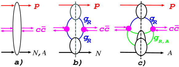
Figure 8: (a) The Kancheli-Mueller diagram for the $c\bar{c}$ jet spectrum, (b) its explicit form in terms of the emission of a $c\bar{c}$ pair off reggeized gluons $g_{R}$ in proton-nucleon collisions, (d) the same as (b) for proton-nucleus collisions in terms of two cut nuclear pomerons ${\bf I\!P}_{A,g}$ composed of effective nuclear reggeized gluons $g_{R,A}$ and the vertex of emission of a $c\bar{c}$ in a transition from reggeized gluon $g_{R}$ to two effective nuclear gluons $g_{R,A}$.

Now, following our early discussion in SingleJet , we comment that the above multiregge form for mid-rapidity, Fig. 7e, is quite likely to be an exclusive property of single gluon production, and the multipomeron version, Fig. 7f, is not an artefact. Indeed, a jet can well be formed by a fixed-mass two-parton or higher multiplicity multiparton state. As an illustration we look at the universality class of mid-rapidity open charm pair $c\bar{c}$ when the transverse momentum much larger than the mass of the diparton. The factorization properties of mid-rapidity $c\bar{c}$ production were studied in QuarkGluonDijet ; Nonuniversality ; Paradigm ; SingleJet . The principal finding is a full fledged nonlinear $k_{\perp}$-factorization for mid-rapidity $c\bar{c}$ production. Consequently, in the corresponding $3\to 3$ Kancheli-Mueller diagram the exchange between the $c\bar{c}$ jet and the target nucleus can not be described by the single nuclear pomeron.

It is sufficient to consider the $g\to c\bar{c}$ excitation and Born cross sections to the large $N_{c}$ approximation. Regarding the color properties, at large $N_{c}$ the $c\bar{c}$ pair is a composite gluon. Let $z$ and $\bar{z}=1-z$ be a partition of the $c\bar{c}$ jet momentum between the quark and antiquark, $p$ the total transverse momentum of the open charm jet, and $k$ the transverse momentum of the quark with respect to the jet, so that

$$M_{\perp,c\bar{c}}^{2}={\mbox{\boldmath$k$}^{2}+m_{c}^{2}\over z(1-z)}+\mbox{\boldmath$p$}^{2}.$$ (128)

The differential form of Eq. (23) of Ref. SingleJet gives the free-nucleon spectrum

$${2(2\pi)^{2}d\sigma_{N}(g^{*}\to c\bar{c})\over dzd^{2}\mbox{\boldmath$p$}d^{2}\mbox{\boldmath$k$}}=2\alpha_{S}P_{qg}(z)f(\mbox{\boldmath$p$})$$

$$\times[K(z\mbox{\boldmath$p$}+\mbox{\boldmath$k$},\mbox{\boldmath$k$})+K((1-z)\mbox{\boldmath$p$}-\mbox{\boldmath$k$},-\mbox{\boldmath$k$})],$$

(129)

Here a square of the vertex of emission of the $c\bar{c}$ pair from a reggeized gluon, $(c\bar{c})g_{R}g_{R}$ in Fig. 8b, is $\propto P_{qg}(z)[K(z\mbox{\boldmath$p$}+\mbox{\boldmath$k$},\mbox{\boldmath$k$})+K((1-z)\mbox{\boldmath$p$}-\mbox{\boldmath$k$},-\mbox{\boldmath$k$})]$. The nuclear $c\bar{c}$ jet spectrum equals

$${2(2\pi)^{2}d\sigma_{A}(g^{*}\to Q\bar{Q})\over d^{2}\mbox{\boldmath$b$}dzd^{2}\mbox{\boldmath$p$}d^{2}\mbox{\boldmath$k$}}=$$

$$=2\alpha_{S}P_{qg}(z)\int d^{2}\mbox{\boldmath$\kappa$}_{1}d^{2}\mbox{\boldmath$\kappa$}_{2}\delta(\mbox{\boldmath$p$}-\mbox{\boldmath$\kappa$}_{1}-\mbox{\boldmath$\kappa$}_{2})$$

$$\times\Phi_{g}(\mbox{\boldmath$b$},x_{A},\mbox{\boldmath$\kappa$}_{1})\Phi_{g}(\mbox{\boldmath$b$},x_{A},\mbox{\boldmath$\kappa$}_{2})$$

$$\times[K(z\mbox{\boldmath$p$}+\mbox{\boldmath$k$}-\mbox{\boldmath$\kappa$}_{1},\mbox{\boldmath$k$})$$

$$+K((1-z)\mbox{\boldmath$p$}-\mbox{\boldmath$k$}-\mbox{\boldmath$\kappa$}_{1},-\mbox{\boldmath$k$})]$$ (130)

and corresponds to the Kancheli-Mueller diagram of Fig. 8c with two cut nuclear pomerons $P_{A,g}$. Then Eq. (130) gives an explicit form of the quark loop contribution to the fully cut triple-pomeron vertex, and a comparison with Eq. (129) suggests a simple correspondence between this triple-pomeron vertex and the square of the $(c\bar{c})g_{R}g_{R}$ vertex. Eq. (130) is the Born approximation, the discussion of LL${1\over x}$ iterations in Sec. V.D suggests that upon the pQCD radiative corrections $\Phi_{g}(\mbox{\boldmath$b$},x_{A},\mbox{\boldmath$\kappa$})\Phi_{g}(\mbox{\boldmath$b$},x_{A},\mbox{\boldmath$\kappa$}_{2})$ is substituted by the LL${1\over x}$ evolved $\Phi_{g}(\mbox{\boldmath$b$},x,\mbox{\boldmath$\kappa$})\Phi_{g}(\mbox{\boldmath$b$},x,\mbox{\boldmath$\kappa$}_{2})$, although this conjecture must be checked.

Finally, we briefly comment on a possible structure of the related Kancheli-Mueller diagrams for digluon jets, a more detailed analysis will be reported elsewhere NSZ_AGK . We recall that the mid-rapidity open charm production belongs to the universality class of nonlinear $k$-factorization which is free of coherent distortions of the dipole wave functions. Also, at large $N_{c}$ it is a single-channel problem. In contrast to that, intranuclear evolution of digluons is a full fledged multichannel non-Abelian problem, the pattern of nonlinear $k$-factorization depends on the color state of digluons and there are coherent distortions of the color dipole wave function which change from one universality class to another and depend on the depth in a nucleus at which digluons in color representations higher than the adjoint representation are excited Nonuniversality ; Paradigm ; GluonGluonDijet . The corresponding Kancheli-Mueller diagrams for digluons will be similar to Fig. 8c complemented by uncut pomeron exchanges on both sides of the unitarity cut, which describe the nuclear distortions of the corresponding partially cut multipomeron vertices. In the universality class of digluons in higher color representations these partially cut multipomeron vertices must be averaged over the depth in a nucleus.

VI Summary and conclusions

We reported a derivation of the transverse momentum dependent LPM effect for leading jets in the beam fragmentation of proton-proton and proton-nucleus collisions. In conjunction with the LL${1\over x}$ evolution for the collective nuclear unintegrated glue, our results offer a basis for a viable pQCD phenomenology of the LPM effect – the radiation driven quenching – of leading jets in $pp$ and $pA$ collisions in the finite energy range from RHIC to LHC.

The first novelty of our work is the derivation of the virtual radiative correction to the spectrum of leading jets. The quenching of forward jets is caused by radiation of hard gluons and, by virtue of the unitarity relation, the opening of the radiation channel is followed by the renormalization of the radiationless process. Our derivation of this renormalization, i.e., of the virtual radiative correction, is based on an explicit solution of the $s$-channel unitarity relation. While for the free-nucleon target both the real emission and virtual radiative corrections are linear $k_{\perp}$-factorizable, for nuclear targets the quantitative description of the LPM effect for forward dijets requires the full-fledged nonlinear $k_{\perp}$-factorization.

The second novelty of our work is an establishment of the LPM effect-deconvoluted, i.e., the LL${1\over x}$ approximation, spectrum of leading partons as a unique linear probe of the collective unintegrated nuclear glue as defined through the excitation of coherent diffractive dijets off nuclei. This must be contrasted to the manifestly nonlinear $k_{\perp}$-factorization for all dijet observables and the LPM effect for single-jet spectra. Although both real-emission and virtual radiative corrections to the leading jet spectrum are described by nonlinear $k_{\perp}$-factorization, our new finding is that this nonlinear $k_{\perp}$-factorization for leading jets exactly matches the equally nonlinear $k_{\perp}$-factorization for the LL${1\over x}$ evolution of the nuclear glue. The two nonlinear evolving observables prove to be proportional to each other: the leading jet production maps linearly the collective nuclear glue. Our focus was on the impact of gluons radiated in the rapidity space between the observed leading jet and the target nucleus, but all our observations on the combined effect of the VRC and REC are fully applicable to production of mid-rapidity jets too. Here our nonlinear $k_{\perp}$ factorization results suggest interesting reggeon field theory properties of the Kancheli-Mueller diagrams for multiparton jets.

For the free-nucleon targets such a linear $k_{\perp}$-factorization for, and the BFKL evolution property of, the leading jet spectrum are valid to all orders of the LL${1\over x}$ BFKL evolution. While the above specified definition of the collective nuclear glue in terms of coherent diffraction off nuclei is viable to all orders of the LL${1\over x}$ evolution, our proof of the linear $k_{\perp}$-factorization for leading jets off nuclei is rigorous only to the first iteration of the LL${1\over x}$ evolution. Even this result is sufficient for the quantitative predictions of the quenching of leading jets at RHIC because of the not so large energy of RHIC. A similar description of the experimental data at the much higher energies of LHC requires several – two to three – steps of the LL${1\over x}$ evolution. We argue that for such a small number of iterations, the treatment of heavy nuclei as a dilute uncorrelated gas of nucleons is still viable, and in the finite energy range from RHIC to LHC, one can perform this evolution in the Balitsky-Kovchegov approximation. After such an evolution, our evaluation of the LPM effect for leading jets will be fully applicable to a comparison of $pp$ and $pA$ collisions at LHC.

Our analysis of the nonlinear $k_{\perp}$-factorization properties of the BK approximation revealed a remarkable feature: the evolution equation can be cast in the form of fully linear BFKL evolution for the collective nuclear glue complemented by a nonlinear term which for hard gluons is a pure higher twist correction. To our opinion, this new form of the evolution is best suited for several iterations needed to bridge the energy range from RHIC to LHC.

We conclude by noting that one process which invites an application of the found linear $k_{\perp}$-factorization for leading jets is the coherent diffractive deep inelastic scattering scattering off nucleons and nuclei. The differential cross section of forward diffractive DIS is a sum of differential cross section of elastic scattering of multiparton Fock states of the photon NZ92 ; NZ94 . As such, diffractive DIS is an inherently nonlinear process to be described by nonlinear $k_{\perp}$-factorization. One can insist, though, on the linear color dipole representation of the diffractive cross section similar to that of inclusive DIS NZ94 ; NSZZdiffrValence . Such a representation would entail a certain nonlinear $k_{\perp}$-factorization form of the unintegrated glue in the pomeron. On the other hand, motivated by the above discussion, one may try to define the glue in the pomeron in terms of the transverse momentum spectrum of leading (anti)quark jets in the high-mass diffractive system. The recent finding is that the two definitions of the unintegrated glue in the pomeron would differ one from another - one must be cautious with the unitarity cut reinterpretation of the color dipole representation for diffraction 3POMglue .

Appendix: Still more linear form of the nonlinear evolution

After we partly vindicated the utility of the BK approximation for finite-energy evolution and heavy nuclei, we report here an interesting alternative form of this equation (the preliminary discussion was reported elsewhere NonlinearBFKL ), which offers a fresh view at the distinction between the linear and genuinely nonlinear components of the evolution equation for the triplet-antitriplet dipoles (LABEL:eq:5.C.5). An obvious drawback of this form is a reference to the explicit Glauber-Gribov form of the nuclear attenuation factor. However, making use of the sum rule $\int d^{2}\mbox{\boldmath$\kappa$}\Phi(\mbox{\boldmath$b$},x_{0},\mbox{\boldmath$\kappa$})=1$, i.e., $\int d^{2}\mbox{\boldmath$\kappa$}\phi(\mbox{\boldmath$b$},x,\mbox{\boldmath$\kappa$})=1-\textsf{S}[\mbox{\boldmath$b$};\sigma_{q\bar{q}0}(x_{0})]$, one can bring it into the form,

$${\partial\phi(\mbox{\boldmath$b$},x,\mbox{\boldmath$p$})\over\partial\log(1/x)} ={\cal{K}}_{BFKL}\otimes\phi(\mbox{\boldmath$b$},x,\mbox{\boldmath$p$})$$ (A.1)

$$+{\cal{Q}}[\phi](\mbox{\boldmath$b$},x,\mbox{\boldmath$p$})\,,$$

where the nonlinear $k_{\perp}$-factorization (quadratic) functional ${\cal{Q}}[\phi]$ is given by

$${\cal{Q}}[\phi](\mbox{\boldmath$b$},x,\mbox{\boldmath$p$}) = \int d^{2}\mbox{\boldmath$q$}d^{2}\mbox{\boldmath$\kappa$}\phi(\mbox{\boldmath$b$},x,\mbox{\boldmath$q$})\Big{\{}\Big{[}K(\mbox{\boldmath$p$}+\mbox{\boldmath$\kappa$},\mbox{\boldmath$p$}+\mbox{\boldmath$q$})-K(\mbox{\boldmath$p$},\mbox{\boldmath$\kappa$}+\mbox{\boldmath$p$})-K(\mbox{\boldmath$p$},\mbox{\boldmath$q$}+\mbox{\boldmath$p$})\Big{]}$$ (A.2)

$$\times \phi(\mbox{\boldmath$b$},x,\mbox{\boldmath$\kappa$})-\phi(\mbox{\boldmath$b$},x,\mbox{\boldmath$p$})\Big{[}K(\mbox{\boldmath$\kappa$},\mbox{\boldmath$\kappa$}+\mbox{\boldmath$q$}+\mbox{\boldmath$p$})-K(\mbox{\boldmath$\kappa$},\mbox{\boldmath$\kappa$}+\mbox{\boldmath$p$})\Big{]}\Big{\}}\,.$$

The first iteration of (A.1) with $x=x_{0}=x_{A}$ in the rhs is exact. The so-defined ${\cal{Q}}[\phi](\mbox{\boldmath$b$},x_{0},\mbox{\boldmath$p$})$ is free of $\textsf{S}[\mbox{\boldmath$b$};\sigma_{0}(x_{0})]$ and we view it as a better candidate for finite-energy iterations as discussed in Sec. V.E. If one would identify $\phi(\mbox{\boldmath$b$},x,\mbox{\boldmath$p$})$ with the exchange by collective nuclear pomeron, then ${\cal{Q}}[\phi]$ describes the fusion of two nuclear pomerons, each of which is a nonlinear functional of, and sums a multiple exchange by, the free-nucleon pomerons.

In the case of the azimuthally symmetric $\phi(\mbox{\boldmath$b$},x,\mbox{\boldmath$p$})$, i.e., the conformal spin zero in the $t$-channel, the nonlinear $k_{\perp}$-factorization functional ${\cal{Q}}[\phi]$ takes a remarkably simple form. In this case the azimuthal averaging can be performed explicitly and leads to enormous simplifications. For instance, when $\varepsilon^{2}$ can be neglected compared to all the momenta, we make use of

$$\Big{\langle}{\mbox{\boldmath$\kappa$}+\mbox{\boldmath$p$}\over(\mbox{\boldmath$\kappa$}+\mbox{\boldmath$p$})^{2}}\Big{\rangle}_{\mbox{\boldmath$\kappa$}} = {\mbox{\boldmath$p$}\over\mbox{\boldmath$p$}^{2}}\,\theta(\mbox{\boldmath$p$}^{2}-\mbox{\boldmath$\kappa$}^{2})\,,$$ (A.3)

the related result for a finite $\varepsilon^{2}$ in the wave function (57) is found in NZ92 ; NZsplit , see also below. Here the subscript indicates the azimuthal angle of the momentum the averaging is performed over.

First we notice that for negligible small $\varepsilon^{2}=\mu_{g}^{2}$

$$K(\mbox{\boldmath$p$}+\mbox{\boldmath$\kappa$},\mbox{\boldmath$p$}+\mbox{\boldmath$q$})-K(\mbox{\boldmath$p$},\mbox{\boldmath$\kappa$}+\mbox{\boldmath$p$})-K(\mbox{\boldmath$p$},\mbox{\boldmath$q$}+\mbox{\boldmath$p$})=$$ (A.4)

$$= 2\Big{[}{\mbox{\boldmath$p$}\over\mbox{\boldmath$p$}^{2}}\cdot{\mbox{\boldmath$\kappa$}+\mbox{\boldmath$p$}\over(\mbox{\boldmath$\kappa$}+\mbox{\boldmath$p$})^{2}}+{\mbox{\boldmath$p$}\over\mbox{\boldmath$p$}^{2}}\cdot{\mbox{\boldmath$q$}+\mbox{\boldmath$p$}\over(\mbox{\boldmath$q$}+\mbox{\boldmath$p$})^{2}}$$

$$- {\mbox{\boldmath$\kappa$}+\mbox{\boldmath$p$}\over(\mbox{\boldmath$\kappa$}+\mbox{\boldmath$p$})^{2}}\cdot{\mbox{\boldmath$q$}+\mbox{\boldmath$p$}\over(\mbox{\boldmath$q$}+\mbox{\boldmath$p$})^{2}}-{1\over\mbox{\boldmath$p$}^{2}}\Big{]}.$$

Upon the averaging over the azimuthal angles of $\kappa$ and $q$ we obtain

$$\Big{\langle}\Big{\langle}K(\mbox{\boldmath$p$}+\mbox{\boldmath$\kappa$},\mbox{\boldmath$p$}+\mbox{\boldmath$q$})-K(\mbox{\boldmath$p$},\mbox{\boldmath$\kappa$}+\mbox{\boldmath$p$})-K(\mbox{\boldmath$p$},\mbox{\boldmath$q$}+\mbox{\boldmath$p$})\Big{\rangle}\Big{\rangle}_{\mbox{\boldmath$q$},\mbox{\boldmath$\kappa$}}=-{2\over\mbox{\boldmath$p$}^{2}}\theta(\mbox{\boldmath$\kappa$}^{2}-\mbox{\boldmath$p$}^{2})\theta(\mbox{\boldmath$q$}^{2}-\mbox{\boldmath$p$}^{2})\,.$$ (A.5)

In the second piece of (A.2) we make first a judicious shift of the integration variable $\kappa$ in the convergent integral: $K(\mbox{\boldmath$\kappa$},\mbox{\boldmath$\kappa$}+\mbox{\boldmath$q$}+\mbox{\boldmath$p$})-K(\mbox{\boldmath$\kappa$},\mbox{\boldmath$\kappa$}+\mbox{\boldmath$p$})\Rightarrow K(\mbox{\boldmath$\kappa$}-\mbox{\boldmath$p$},\mbox{\boldmath$\kappa$}+\mbox{\boldmath$q$})-K(\mbox{\boldmath$\kappa$},\mbox{\boldmath$\kappa$}+\mbox{\boldmath$p$})$. Next, we perform the averaging over the azimuthal angles of $q$ and the external variable $p$. There emerges the convergent, and vanishing, integral

$$\int d^{2}\mbox{\boldmath$\kappa$}\Biggl{[}{1\over\mbox{\boldmath$\kappa$}^{2}}-{1\over(\mbox{\boldmath$\kappa$}+\mbox{\boldmath$q$})^{2}}\Biggr{]}=0.$$ (A.6)

Upon this cancellation, for negligible small $\varepsilon^{2}$,

$$\Big{\langle}\Big{\langle}K(\mbox{\boldmath$\kappa$}-\mbox{\boldmath$p$},\mbox{\boldmath$\kappa$}+\mbox{\boldmath$q$})-K(\mbox{\boldmath$\kappa$},\mbox{\boldmath$\kappa$}+\mbox{\boldmath$p$})\Big{\rangle}\Big{\rangle}_{\mbox{\boldmath$p$},\mbox{\boldmath$q$}}=$$ (A.7)

$$= 2\Big{\langle}\Big{\langle}{\mbox{\boldmath$\kappa$}\over\mbox{\boldmath$\kappa$}^{2}}\cdot{\mbox{\boldmath$\kappa$}+\mbox{\boldmath$p$}\over(\mbox{\boldmath$\kappa$}+\mbox{\boldmath$p$})^{2}}-{\mbox{\boldmath$\kappa$}-\mbox{\boldmath$p$}\over(\mbox{\boldmath$\kappa$}-\mbox{\boldmath$p$})^{2}}\cdot{\mbox{\boldmath$\kappa$}+\mbox{\boldmath$q$}\over(\mbox{\boldmath$\kappa$}+\mbox{\boldmath$q$})^{2}}\Big{\rangle}\Big{\rangle}_{\mbox{\boldmath$p$},\mbox{\boldmath$q$}}$$

$$= {2\over\mbox{\boldmath$\kappa$}^{2}}\theta(\mbox{\boldmath$\kappa$}^{2}-\mbox{\boldmath$p$}^{2})\theta(\mbox{\boldmath$q$}^{2}-\mbox{\boldmath$\kappa$}^{2})\,$$

Putting it all together the quadratic functional ${\cal{Q}}[\phi]$ assumes the very simple form,

$${\cal{Q}}[\phi](\mbox{\boldmath$b$},x,\mbox{\boldmath$p$}) = -{2{\cal K}_{0}\over\mbox{\boldmath$p$}^{2}}\int d^{2}\mbox{\boldmath$q$}d^{2}\mbox{\boldmath$\kappa$}\phi(\mbox{\boldmath$b$},x,\mbox{\boldmath$q$})\phi(\mbox{\boldmath$b$},x,\mbox{\boldmath$p$})\theta(\mbox{\boldmath$q$}^{2}-\mbox{\boldmath$p$}^{2})\theta(\mbox{\boldmath$\kappa$}^{2}-\mbox{\boldmath$p$}^{2})$$

$$-2{\cal K}_{0}\phi(\mbox{\boldmath$b$},x,\mbox{\boldmath$p$})\int{d^{2}\mbox{\boldmath$\kappa$}\over\mbox{\boldmath$\kappa$}^{2}}\int d^{2}\mbox{\boldmath$q$}\phi(\mbox{\boldmath$b$},x,\mbox{\boldmath$q$})\theta(\mbox{\boldmath$\kappa$}^{2}-\mbox{\boldmath$p$}^{2})\theta(\mbox{\boldmath$q$}^{2}-\mbox{\boldmath$\kappa$}^{2})$$

$$=-{2{\cal K}_{0}\over\mbox{\boldmath$p$}^{2}}\Biggl{[}\int_{\mbox{\boldmath$p$}^{2}}^{\infty}d^{2}\mbox{\boldmath$q$}\phi(\mbox{\boldmath$b$},x,\mbox{\boldmath$q$})\Biggr{]}^{2}-2{\cal K}_{0}\phi(\mbox{\boldmath$b$},x,\mbox{\boldmath$p$})\int_{\mbox{\boldmath$p$}^{2}}^{\infty}{d^{2}\mbox{\boldmath$\kappa$}\over\mbox{\boldmath$\kappa$}^{2}}\int_{\mbox{\boldmath$\kappa$}^{2}}^{\infty}d^{2}\mbox{\boldmath$q$}\phi(\mbox{\boldmath$b$},x,\mbox{\boldmath$q$}),$$

valid for the transverse momenta larger than the infrared regularization $\mu_{g}$, for the effects of finite $\mu_{g}$ see equations (LABEL:eq:Append.15 - LABEL:eq:Append.19) below.

It is instructive to reformulate it in terms of the collective nuclear glue per bound nucleon, ${\cal F}_{A}(\mbox{\boldmath$b$},x,\mbox{\boldmath$p$})$:

$$\phi(\mbox{\boldmath$b$},x,\mbox{\boldmath$p$})={2\pi\alpha_{S}(\mbox{\boldmath$p$}^{2})\over N_{c}p^{4}}T(\mbox{\boldmath$b$}){\cal F}_{A}(\mbox{\boldmath$b$},x,\mbox{\boldmath$p$}).$$ (A.9)

One readily obtains

$${\partial{\cal F}_{A}(\mbox{\boldmath$b$},x,\mbox{\boldmath$p$})\over\partial\log{1\over x}}={\partial^{2}G_{A}(\mbox{\boldmath$b$},x,\mbox{\boldmath$p$})\over\partial\log\mbox{\boldmath$p$}^{2}\partial\log{1\over x}}$$

$$= {\cal K}_{BFKL}\otimes{\cal F}_{A}(\mbox{\boldmath$b$},x,\mbox{\boldmath$p$})$$

$$- {4\pi{\cal K}_{0}\over N_{c}}\alpha_{S}(\mbox{\boldmath$p$}^{2})T(\mbox{\boldmath$b$})\Biggl{\{}\mbox{\boldmath$p$}^{2}\Bigl{[}\int_{\mbox{\boldmath$p$}^{2}}^{\infty}{d^{2}\mbox{\boldmath$q$}\over q^{4}}{\cal F}_{A}(\mbox{\boldmath$b$},x,\mbox{\boldmath$q$})\Bigr{]}^{2}$$

$$+ {\cal F}_{A}(\mbox{\boldmath$b$},x,\mbox{\boldmath$p$})\int_{\mbox{\boldmath$p$}^{2}}^{\infty}{d^{2}\mbox{\boldmath$\kappa$}\over\mbox{\boldmath$\kappa$}^{2}}\int_{\mbox{\boldmath$\kappa$}^{2}}^{\infty}{d^{2}\mbox{\boldmath$q$}\over q^{4}}{\cal F}_{A}(\mbox{\boldmath$b$},x,\mbox{\boldmath$q$})\Biggr{\}},$$

The fusion term is of manifestly negative, i.e., shadowing, sign. As such, Eq. (A.2) is the better candidate for the definition of of the triple-pomeron vertex for nuclear pomerons than Eq. (LABEL:eq:5.C.5). Such a representation for the fusion term is a new result, it is exact for all momenta, both above the saturation scale, $\mbox{\boldmath$p$}^{2}\mathrel{\hbox to0.0pt{\lower 4.0pt\hbox{\hskip 1.0pt$\sim$}\hss}\raise 1.0pt\hbox{$>$}}Q_{A}^{2}$, and under the saturation scale, $\mbox{\boldmath$p$}^{2}\mathrel{\hbox to0.0pt{\lower 4.0pt\hbox{\hskip 1.0pt$\sim$}\hss}\raise 1.0pt\hbox{$<$}}Q_{A}^{2}$, provided that $\mbox{\boldmath$p$}^{2}\mathrel{\hbox to0.0pt{\lower 4.0pt\hbox{\hskip 1.0pt$\sim$}\hss}\raise 1.0pt\hbox{$>$}}\mu_{g}^{2}$.

Now we shall argue that at large momenta above the the saturation scale the fusion term is of pure higher twist. We focus on $x=x_{0}$, where one can rely upon the saturation, antishadowing and hard momentum properties of $\phi(\mbox{\boldmath$b$},x_{0},\mbox{\boldmath$p$})$ found in NSSdijet ; Nonlinear ; SingleJet . Here we need the large-momentum approximation

$$\phi(\mbox{\boldmath$b$},x_{0},\mbox{\boldmath$p$}) \approx {1\over 2}T(\mbox{\boldmath$b$})f(x_{0},\mbox{\boldmath$p$})\propto{1\over(\mbox{\boldmath$p$}^{2})^{\gamma}}$$

where the exponent $\gamma\approx 2$, see Eq. (14). Making the explicit use of this asymptotic behavior, we obtain

$${1\over\mbox{\boldmath$p$}^{2}}\Biggl{[}\int_{\mbox{\boldmath$p$}^{2}}^{\infty}d^{2}\mbox{\boldmath$q$}\phi(\mbox{\boldmath$b$},x_{0},\mbox{\boldmath$q$})\Biggr{]}^{2}\approx$$

$$\approx\phi(\mbox{\boldmath$b$},x_{0},\mbox{\boldmath$p$})\int_{\mbox{\boldmath$p$}^{2}}^{\infty}{d^{2}\mbox{\boldmath$\kappa$}\over\mbox{\boldmath$\kappa$}^{2}}\int_{\mbox{\boldmath$\kappa$}^{2}}^{\infty}d^{2}\mbox{\boldmath$q$}\phi(\mbox{\boldmath$b$},x_{0},\mbox{\boldmath$q$})$$

$$\approx{\pi^{2}\over(\gamma-1)^{2}}\mbox{\boldmath$p$}^{2}\phi^{2}(\mbox{\boldmath$b$},x_{0},\mbox{\boldmath$p$}^{2}).$$ (A.12)

The fusion term takes the form of the boundary condition glue times the higher twist factor,

$${\cal{Q}}[\phi](\mbox{\boldmath$b$},x_{0},\mbox{\boldmath$p$})\approx$$ (A.13)

$$- {4\pi^{2}{\cal K}_{0}\over(\gamma-1)^{2}}\phi(\mbox{\boldmath$b$},x_{0},\mbox{\boldmath$p$})\cdot\{\mbox{\boldmath$p$}^{2}\phi(\mbox{\boldmath$b$},x_{0},\mbox{\boldmath$p$})\}$$

$$\approx {2\pi\alpha_{S}(\mbox{\boldmath$p$}^{2})\over(\gamma-1)^{2}\alpha_{S}(Q_{A}^{2}(\mbox{\boldmath$b$},x_{0}))G(x_{0},Q_{A}^{2}(\mbox{\boldmath$b$},x_{0}))}$$

$$\times {Q_{A}^{2}(\mbox{\boldmath$b$},x_{0})\over\mbox{\boldmath$p$}^{2}}\cdot\phi(\mbox{\boldmath$b$},x_{0},\mbox{\boldmath$p$}^{2}),$$

where the scale for the higher twist is set by the saturation scale. In terms of the collective glue per bound nucleon, this amounts to

$${\partial{\cal F}_{A}(\mbox{\boldmath$b$},x,\mbox{\boldmath$p$})\over\partial\log{1\over x}}={\cal K}_{BFKL}\otimes{\cal F}_{A}(\mbox{\boldmath$b$},x_{0},\mbox{\boldmath$p$})$$

$$- {8{\cal K}_{0}\pi^{3}\alpha_{S}(\mbox{\boldmath$p$}^{2})T(\mbox{\boldmath$b$})\over(\gamma-1)^{2}N_{c}\mbox{\boldmath$p$}^{2}}{\cal F}_{A}^{2}(\mbox{\boldmath$b$},x_{0},\mbox{\boldmath$p$}).$$

In contrast to the exact integral form (LABEL:eq:Append.10) of the fusion term, the local in the gluon momentum form (LABEL:eq:Append.14) is an approximation valid for the specific parameterization (LABEL:eq:Append.11), for alternative forms of the fusion correction see GLR ; MuellerQiu . The further discussion of (LABEL:eq:Append.10) and (LABEL:eq:Append.14) goes beyond the scope of this communication. We restrict ourselves to the comment that the fusion term does not exhaust the nuclear higher twist corrections – we recall that also the boundary condition ${\cal F}_{A}(\mbox{\boldmath$b$},x_{0},\mbox{\boldmath$p$}^{2})$ contains a substantial and very similar, but positive valued, i.e., antishadowing, linear BFKL-evolving nuclear higher twist correction proportional to ${\cal F}_{A}(\mbox{\boldmath$b$},x_{0},\mbox{\boldmath$p$}^{2})G_{A}(\mbox{\boldmath$b$},x_{0},Q^{2})T(\mbox{\boldmath$b$})/\mbox{\boldmath$p$}^{2}$ NSSdijet ; NSSdijetJETPLett ; Nonlinear . The shadowing and antishadowing nuclear higher twist corrections both have their origin in unitarity, the impact of the antishadowing correction was not given a proper discussion earlier.

For the sake of completeness, we show the integral form of the fusion term in Eq. (LABEL:eq:Append.10) subject to the infrared regularization (85), i.e. in all wave functions, $K(\mbox{\boldmath$p$},\mbox{\boldmath$q$})$ and ${\cal K}_{BFKL}$ we put $\varepsilon^{2}=\mu_{g}^{2}$. Following NZ92 ; NZsplit we can write

$$\Big{\langle}{\mbox{\boldmath$\kappa$}+\mbox{\boldmath$p$}\over(\mbox{\boldmath$\kappa$}+\mbox{\boldmath$p$})^{2}+\mu_{g}^{2}}\Big{\rangle}_{\mbox{\boldmath$\kappa$}} = {\mbox{\boldmath$p$}\over\mbox{\boldmath$p$}^{2}+\mu_{g}^{2}}\,\theta(\mbox{\boldmath$p$}^{2},\mbox{\boldmath$\kappa$}^{2},\mu_{g}^{2}),$$

where

$$\theta(\mbox{\boldmath$p$}^{2},\mbox{\boldmath$\kappa$}^{2},\mu_{g}^{2})={\mbox{\boldmath$p$}^{2}+\mu_{g}^{2}\over 2\mbox{\boldmath$p$}^{2}}$$

$$\times\left(1+{\mbox{\boldmath$p$}^{2}-\mu_{g}^{2}-\mbox{\boldmath$\kappa$}^{2}\over\sqrt{(\mbox{\boldmath$p$}^{2}-\mu_{g}^{2}-\mbox{\boldmath$\kappa$}^{2})^{2}+4\mbox{\boldmath$p$}^{2}\mu_{g}^{2}}}\right).$$

(A.16)

Eqs. (A.5) and  (A.5) take the form

$$\Big{\langle}\Big{\langle}K(\mbox{\boldmath$p$}+\mbox{\boldmath$\kappa$},\mbox{\boldmath$p$}+\mbox{\boldmath$q$})-K(\mbox{\boldmath$p$},\mbox{\boldmath$\kappa$}+\mbox{\boldmath$p$})-K(\mbox{\boldmath$p$},\mbox{\boldmath$q$}+\mbox{\boldmath$p$})\Big{\rangle}\Big{\rangle}_{\mbox{\boldmath$q$},\mbox{\boldmath$\kappa$}}=$$ (A.17)

$$= -{2\mbox{\boldmath$p$}^{2}\over(\mbox{\boldmath$p$}^{2}+\mu_{g}^{2})^{2}}[1-\theta(\mbox{\boldmath$p$}^{2},\mbox{\boldmath$\kappa$}^{2},\mu_{g}^{2})][1-\theta(\mbox{\boldmath$p$}^{2},\mbox{\boldmath$q$}^{2},\mu_{g}^{2})],$$

$$\Big{\langle}\Big{\langle}K(\mbox{\boldmath$\kappa$}-\mbox{\boldmath$p$},\mbox{\boldmath$\kappa$}+\mbox{\boldmath$q$})-K(\mbox{\boldmath$\kappa$},\mbox{\boldmath$\kappa$}+\mbox{\boldmath$p$})\Big{\rangle}\Big{\rangle}_{\mbox{\boldmath$p$},\mbox{\boldmath$q$}}={2\mbox{\boldmath$\kappa$}^{2}\over(\mbox{\boldmath$\kappa$}^{2}+\mu_{g}^{2})^{2}}\theta(\mbox{\boldmath$\kappa$}^{2},\mbox{\boldmath$p$}^{2},\mu_{g}^{2})[1-\theta(\mbox{\boldmath$\kappa$}^{2},\mbox{\boldmath$q$}^{2},\mu_{g}^{2})].$$ (A.18)

The infrared-regularization modifies the evolution equation (LABEL:eq:Append.10) as follows:

$${\partial{\cal F}_{A}(\mbox{\boldmath$b$},x,\mbox{\boldmath$p$})\over\partial\log{1\over x}} = {\cal K}_{BFKL}\otimes{\cal F}_{A}(\mbox{\boldmath$b$},x,\mbox{\boldmath$p$})$$

$$- {4\pi{\cal K}_{0}\over N_{c}}\alpha_{S}(\mbox{\boldmath$p$}^{2})T(\mbox{\boldmath$b$})\Biggl{\{}{p^{6}\over(\mbox{\boldmath$p$}^{2}+\mu_{g}^{2})^{2}}\Bigl{[}\int{d^{2}\mbox{\boldmath$q$}\over q^{4}}[1-\theta(\mbox{\boldmath$p$}^{2},\mbox{\boldmath$q$}^{2},\mu_{g}^{2})]{\cal F}_{A}(\mbox{\boldmath$b$},x,\mbox{\boldmath$q$})\Bigr{]}^{2}$$

$$+ {\cal F}_{A}(\mbox{\boldmath$b$},x,\mbox{\boldmath$p$})\int\int{d^{2}\mbox{\boldmath$\kappa$}d^{2}\mbox{\boldmath$q$}\over(\mbox{\boldmath$\kappa$}^{2}+\mu_{g}^{2})^{2}q^{4}}\theta(\mbox{\boldmath$\kappa$}^{2},\mbox{\boldmath$p$}^{2},\mu_{g}^{2})[1-\theta(\mbox{\boldmath$\kappa$}^{2},\mbox{\boldmath$q$}^{2},\mu_{g}^{2})]{\cal F}_{A}(\mbox{\boldmath$b$},x,\mbox{\boldmath$q$})\Biggr{\}}.$$

References

- (1) B. G. Zakharov, JETP Lett. 63 (1996) 952; JETP Lett. 65 (1997) 615; Phys. Atom. Nucl. 61 (1998) 838 [Yad. Fiz. 61 (1998) 924].
- (2) R. Baier, D. Schiff and B. G. Zakharov, Ann. Rev. Nucl. Part. Sci. 50 (2000) 37.
- (3) J. Jalilian-Marian and Y. V. Kovchegov, Prog. Part. Nucl. Phys. 56, 104 (2006).
- (4) E. Leader and E. Predazzi, Introduction to Gauge Theories and Modern Particle Physics, vols.1 & 2, Cambridge University Press, Cambridge, 1996; G. Sterman, An Introduction to Quantum Field Theory, Cambridge University Press, Cambridge, 1993; R. K. Ellis, W. J. Stirling and B. R. Webber, “QCD and collider physics,” Cambridge Monogr. Part. Phys. Nucl. Phys. Cosmol. 8, 1 (1996).
- (5) J. C. Collins and X. Zu, JHEP 0503, 059 (2005); J. Collins and H. Jung, arXiv:hep-ph/0508280.
- (6) V. S. Fadin, E. A. Kuraev and L. N. Lipatov, Phys. Lett. B 60, 50 (1975); E. A. Kuraev, L. N. Lipatov and V. S. Fadin, Sov. Phys. JETP 45, 199 (1977); [Zh. Eksp. Teor. Fiz. 72, 377 (1977)].
- (7) I. I. Balitsky and L. N. Lipatov, Sov. J. Nucl. Phys. 28, 822 (1978); [Yad. Fiz. 28, 1597 (1978)].
- (8) B. Andersson et al. [Small x Collaboration], Eur. Phys. J. C 25, 77 (2002); J. R. Andersen et al. [Small x Collaboration], Eur. Phys. J. C 35, 67 (2004).
- (9) A. Szczurek, Acta Phys. Polon. B 34, 3191 (2003).
- (10) N. N. Nikolaev, W. Schäfer, B. G. Zakharov and V. R. Zoller, J. Exp. Theor. Phys. 97, 441 (2003); [Zh. Eksp. Teor. Fiz. 124, 491 (2003)].
- (11) N. N. Nikolaev, W. Schäfer, B. G. Zakharov and V. R. Zoller, Phys. At. Nucl. 68, 661 (2005); [Yad. Fiz. 68, 692 (2005)].
- (12) N. N. Nikolaev, W. Schäfer, B. G. Zakharov and V. R. Zoller, Phys. Rev. D 72, 034033 (2005).
- (13) N. N. Nikolaev, W. Schäfer and B. G. Zakharov, Phys. Rev. Lett. 95, 221803 (2005).
- (14) N. N. Nikolaev, W. Schäfer and B. G. Zakharov, Phys. Rev. D 72, 114018 (2005).
- (15) N. N. Nikolaev, W. Schäfer, B. G. Zakharov and V. R. Zoller, JETP Lett. 82, 325 (2005) [Pisma Zh. Eksp. Teor. Fiz. 82, 364 (2005)].
- (16) I. Arsene et al. [BRAHMS Collaboration], Phys. Rev. Lett. 93, 242303 (2004) J. J. Gaardhoje et al. [BRAHMS Collaboration], Eur. Phys. J. C 43, 287 (2005).
- (17) N. N. Nikolaev and W. Schäfer, Phys. Rev. D 71, 014023 (2005).
- (18) J. Jalilian-Marian and Y. V. Kovchegov, Phys. Rev. D 70, 114017 (2004) [Erratum-ibid. D 71, 079901 (2005)].
- (19) J. P. Blaizot, F. Gelis and R. Venugopalan, Nucl. Phys. A 743, 57 (2004).
- (20) R. Baier, A. Kovner, M. Nardi and U. A. Wiedemann, Phys. Rev. D 72, 094013 (2005).
- (21) V. S. Fadin, R. Fiore, M. G. Kozlov and A. V. Reznichenko, arXiv: hep-ph/0602006.
- (22) L. D. McLerran and R. Venugopalan, Phys. Rev. D 49 (1994) 2233; J. Jalilian-Marian, A. Kovner, L. D. McLerran and H. Weigert, Phys. Rev. D 55 (1997) 5414; A. H. Mueller, “Parton saturation: An overview,” QCD perspectives on hot and dense matter, NATO science series II: Mathematics, physics and chemistry, v. 87, edited by J.-P. Blaizot and E. Iancu, Dordrecht, Netherlands: Kluwer Academic (2002); E. Iancu, A. Leonidov and L. McLerran, “The colour glass condensate: An introduction,” QCD perspectives on hot and dense matter, NATO science series II: Mathematics, physics and chemistry, v. 87, edited by J.-P. Blaizot and E. Iancu, Dordrecht, Netherlands: Kluwer Academic (2002); E. Iancu and R. Venugopalan, “The color glass condensate and high energy scattering in QCD,” Quark gluon plasma 3, edited by R.C Hwa and X.N. Wang, Singapore: World Scientific (2004).
- (23) H. Fujii, F. Gelis and R. Venugopalan, Phys. Rev. Lett. 95, 162002 (2005); Eur. Phys. J. C 43, 139 (2005).
- (24) N. N. Nikolaev, W. Schäfer and G. Schwiete, Phys. Rev. D 63, 014020 (2001).
- (25) N. N. Nikolaev, W. Schäfer and G. Schwiete, JETP Lett. 72, 405 (2000). [Pisma Zh. Eksp. Teor. Fiz. 72, 583 (2000)].
- (26) N. N. Nikolaev and B. G. Zakharov, Phys. Lett. B 332, 177 (1994).
- (27) J. C. Collins, Acta Phys. Polon. B 34, 3103 (2003)
- (28) A. Kovner, Acta Phys. Polon. B 36, 3551 (2005) D. N. Triantafyllopoulos, Acta Phys. Polon. B 36, 3593 (2005);
- (29) I. Balitsky, Nucl. Phys. B 463, 99 (1996).
- (30) Y. V. Kovchegov, Phys. Rev. D 60, 034008 (1999).
- (31) N. N. Nikolaev, W. Schäfer, B. G. Zakharov and V. R. Zoller, Proceedings of Workshop on Hadron Structure and QCD: From Low to High Energies (HSQCD 2004), St. Petersburg, Repino, Russia, 18-22 May 2004. arXiv: hep-ph/0501002; N. N. Nikolaev, International Workshop on Diffraction in High-Energy Physics, Cala Gonone, Sardinia, Italy, 18-23 Sep 2004 Nucl. Phys. Proc. Suppl. 146, 220 (2005).
- (32) V. N. Gribov and L. N. Lipatov, Sov. J. Nucl. Phys. 15, 438 (1972) [Yad. Fiz. 15, 781 (1972)]; L. N. Lipatov, Sov. J. Nucl. Phys. 20 (1975) 94 [Yad. Fiz. 20 (1974) 181]. G. Altarelli and G. Parisi, Nucl. Phys. B 126, 298 (1977); Y. L. Dokshitzer, Sov. Phys. JETP 46, 641 (1977) [Zh. Eksp. Teor. Fiz. 73, 1216 (1977)].
- (33) E. M. Levin, M. G. Ryskin, Y. M. Shabelski and A. G. Shuvaev, Sov. J. Nucl. Phys. 53, 657 (1991) [Yad. Fiz. 53, 1059 (1991)]; S. Catani, M. Ciafaloni and F. Hautmann, Nucl. Phys. B 366, 135 (1991). J. C. Collins and R. K. Ellis, Nucl. Phys. B 360, 3 (1991).
- (34) N. N. Nikolaev and B. G. Zakharov, Phys. Lett. B 332, 184 (1994).
- (35) I. P. Ivanov and N. N. Nikolaev, Phys. Atom. Nucl. 64 (2001) 753 [Yad. Fiz. 64 (2001) 813]; Phys. Rev. D 65 (2002) 054004
- (36) B. G. Zakharov, Yad. Fiz. 46, 148 (1987) [Sov. J. Nucl. Phys. 46, 92 (1987)].
- (37) N. N. Nikolaev, G. Piller and B. G. Zakharov, J. Exp. Theor. Phys. 81 (1995) 851 [Zh. Eksp. Teor. Fiz. 108 (1995) 1554]; Z. Phys. A 354 (1996) 99.
- (38) N. N. Nikolaev and B. G. Zakharov, J. Exp. Theor. Phys. 78, 598 (1994); [Zh. Eksp. Teor. Fiz. 105, 1117 (1994)]; N. N. Nikolaev and B. G. Zakharov, Z. Phys. C 64, 631 (1994).
- (39) N. N. Nikolaev, B. G. Zakharov and V. R. Zoller, JETP Lett. 59, 6 (1994).
- (40) N.N. Nikolaev and V.I. Zakharov, Sov. J. Nucl. Phys. 21, 227 (1975) [Yad. Fiz. 21, 434 (1975)]. Phys. Lett. B 55, 397 (1975).
- (41) R. J. Glauber, in Lectures in Theoretical Physics, edited by W. E. Brittin et al. (Interscience Publishers, Inc., New York, 1959), Vol. 1, p. 315.
- (42) V. N. Gribov, Sov. Phys. JETP 29, 483 (1969); [Zh. Eksp. Teor. Fiz. 56, 892 (1969)].
- (43) N. N. Nikolaev, W. Schäfer, B. G. Zakharov and V. R. Zoller, JETP Lett. 76, 195 (2002); [Pisma Zh. Eksp. Teor. Fiz. 76, 231 (2002)].
- (44) E.V. Shuryak, Rev. Mod. Phys. 65, 1 (1993); E. Meggiolaro, Phys. Lett. B 451, 414 (1999);J. H. Field, Phys. Rev. D 66, 013013 (2002).
- (45) K. Rummukainen and H. Weigert, Nucl. Phys. A 739, 183 (2004); A. H. Mueller and A. I. Shoshi, Nucl. Phys. B 692, 175 (2004); A. H. Mueller, A. I. Shoshi and S. M. H. Wong, Nucl. Phys. B 715, 440 (2005); N. Armesto and J. G. Milhano, Phys. Rev. D 73, 114003 (2006).
- (46) N. N. Nikolaev, J. Speth and V. R. Zoller, Phys. Lett. B 473, 157 (2000).
- (47) N. N. Nikolaev, B. G. Zakharov and V. R. Zoller, J. Exp. Theor. Phys. 78, 806 (1994) [Zh. Eksp. Teor. Fiz. 105, 1498 (1994)].
- (48) N. N. Nikolaev, B. G. Zakharov and V. R. Zoller, Phys. Lett. B 328, 486 (1994).
- (49) D. Ashery, Prog. Part. Nucl. Phys. 56, 279 (2006).
- (50) J. Breitweg et al. [ZEUS Collaboration], Eur. Phys. J. C 7, 609 (1999); C. Adloff et al. [H1 Collaboration], Phys. Lett. B 520, 183 (2001).
- (51) M. M. Block and R. N. Cahn, Rev. Mod. Phys. 57, 563 (1985). M. M. Block, E. M. Gregores, F. Halzen and G. Pancheri, Phys. Rev. D 60, 054024 (1999)
- (52) A. B. Kaidalov, Phys. Usp. 46, 1121 (2003) [Usp. Fiz. Nauk 46, 1153 (2003)].
- (53) L. N. Lipatov, Nucl. Phys. B 452, 369 (1995); E. N. Antonov, L. N. Lipatov, E. A. Kuraev and I. O. Cherednikov, Nucl. Phys. B 721, 111 (2005)
- (54) Y. V. Kovchegov and A. H. Mueller, Nucl. Phys. B 529, 451 (1998); Y. V. Kovchegov and K. Tuchin, Phys. Rev. D 65, 074026 (2002).
- (55) O. V. Kancheli, JETP Lett. 11, 267 (1970) [ZhETF Pis. Red. 11, 397 (1970)]; V. A. Abramovsky, O. V. Kancheli and I. D. Mandzhavidze, Yad. Fiz. 13 (1971) 1102; A. H. Mueller, Phys. Rev. D 2 (1970) 2963.
- (56) I. Balitsky, Phys. Rev. D 70, 114030 (2004)
- (57) V. A. Abramovsky, V. N. Gribov and O. V. Kancheli, Yad. Fiz. 18, 595 (1973) [Sov. J. Nucl. Phys. 18, 308 (1974)].
- (58) N. N. Nikolaev, W. Schäfer, B. G. Zakharov and V. R. Zoller, arXiv:hep-ph/0511285.
- (59) N. N. Nikolaev, W. Schäfer and B. G. Zakharov, paper in preparation.
- (60) A. Capella, A. Kaidalov and J. Tran Thanh Van, Heavy Ion Phys. 9, 169 (1999)
- (61) M. A. Braun, Eur. Phys. J. C 42, 169 (2005)
- (62) M. A. Braun, arXiv:hep-ph/0603060.
- (63) N. N. Nikolaev, W. Schäfer, B. G. Zakharov and V. R. Zoller, JETP Lett. 83, 192 (2006).
- (64) N. N. Nikolaev and B. G. Zakharov, Z. Phys. C 53, 331 (1992).
- (65) N. N. Nikolaev, W. Schäfer, B. G. Zakharov and V. R. Zoller, JETP Lett. 80, 371 (2004) [Pisma Zh. Eksp. Teor. Fiz. 80, 423 (2004)].
- (66) L. V. Gribov, E. M. Levin and M. G. Ryskin, Phys. Rept. 100, 1 (1983).
- (67) A. H. Mueller and J. W. Qiu, Nucl. Phys. B 268, 427 (1986).