Abstract

Two of the most important and pressing questions in cosmology and particle physics are: (1) What is the nature of cold dark matter? and (2) Will near-future experiments on neutrinoless double beta decay be able to ascertain that the neutrino is a Majorana particle, i.e. its own antiparticle? We show that these two seemingly unrelated issues are intimately connected if neutrinos acquire mass only because of their interactions with dark matter.

The existence of cold dark matter in the Universe is now well accepted [1]. From the viewpoint of particle physics, it should consist of a weakly interacting yet-to-be-discovered neutral stable fermion or boson. A prime candidate is the lightest supersymmetric particle (LSP) in the minimal supersymmetric standard model (MSSM). More generally, we need only an exactly conserved $Z_{2}$ symmetry [2, 3] and some new particles which are odd under it, keeping all known particles even. In the MSSM, this $Z_{2}$ symmetry is called $R$ parity, and the new particles are the squarks, sleptons, gauginos, and higgsinos.

Consider now the interactions of the neutrino with particles in this new class. To realize the well-known dimension-five operator for Majorana neutrino mass [4],

$${\cal L}_{eff}={f_{\alpha\beta}\over\Lambda}(\nu_{\alpha}\phi^{0}-l_{\alpha}\phi^{+})(\nu_{\beta}\phi^{0}-l_{\beta}\phi^{+})+H.c.,$$ (1)

where $(\nu_{\alpha},l_{\alpha})$ and $\Phi=(\phi^{+},\phi^{0})$ are the usual lepton and Higgs doublets of the standard model (SM), it is clear that the new particles must form a loop with four external legs given by $\nu_{\alpha}\nu_{\beta}\phi^{0}\phi^{0}$. There are generically three such one-loop diagrams [5]. In the MSSM, this does not happen because this operator also requires lepton number to change by two units. However, if a neutral singlet superfield $N$ is added, then Figure 1 is generated as a radiative contribution to the neutrino mass.

Figure 1: One-loop radiative neutrino mass in supersymmetry.

We note that the particles in the loop all have odd $R$ parity. Of course, in the context of supersymmetry, this also implies that $\nu$ couples to $N$ directly through $\phi_{u}^{0}$, so that a Dirac mass already appears, and together with the heavy Majorana mass of $N$, the famous seesaw mechanism [6] allows $\nu$ to obtain a tree-level Majorana mass. That is why Figure 1 is always negligible in the MSSM with the addition of $N$. However, in a more general framework, the new particles in the loop may be the only source of neutrino mass [7, 8], and in that case there will be interesting phenomenological implications on lepton flavor transitions and neutrinoless double beta decay, as shown below.

Basically, the argument goes as follows. In order for the new particles in the loop to be identified as cold dark matter with the correct value of their relic density in the Universe at present, their interactions with neutrinos and charged leptons must not be too weak. On the other hand, they are also responsible for the masses of neutrinos and their observed mixing in neutrino oscillations. This implies necessarily flavor changing transitions such as $\mu\to e\gamma$. In order to suppress the latter, the parameter space of neutrino masses is limited, thereby enforcing a lower bound on neutrinoless double beta decay.

Of the three generic one-loop diagrams giving rise to a radiative neutrino mass, the simplest in terms of new particle content is given in Ref. [8]. The standard model is extended by adding three neutral singlet fermions $N_{i}$ and a second scalar doublet $(\eta^{+},\eta^{0})$, which are odd under an exactly conserved $Z_{2}$ symmetry, keeping all SM particles even. In that case, the analog of Figure 1 is Figure 2, as depicted below.

Figure 2: One-loop radiative neutrino mass in the model of Ref. [8].

We note again that the particles in the loop are all odd, and that lepton number changes by two units as in Figure 1. The $Z_{2}$ invariant Higgs potential is given by

$$V = m_{1}^{2}\Phi^{{\dagger}}\Phi+m_{2}^{2}\eta^{{\dagger}}\eta+\frac{1}{2}\lambda_{1}(\Phi^{{\dagger}}\Phi)^{2}+\frac{1}{2}\lambda_{2}(\eta^{{\dagger}}\eta)^{2}+\lambda_{3}(\Phi^{{\dagger}}\Phi)(\eta^{{\dagger}}\eta)$$ (2)

$$+~{}\lambda_{4}(\Phi^{{\dagger}}\eta)(\eta^{{\dagger}}\Phi)+\frac{1}{2}\lambda_{5}[(\Phi^{{\dagger}}\eta)^{2}+H.c.],$$

with $\langle\phi^{0}\rangle=v$ and $\langle\eta^{0}\rangle=0$. Let us choose the bases where $N_{i}$ and $l_{\alpha},l^{c}_{\alpha}$ are diagonal, and consider the interactions of $(\nu_{\alpha},l_{\alpha})$ with $N_{i}$ and $(\eta^{+},\eta^{0})$, i.e.

$${\cal L}_{N} = h_{\alpha i}(\nu_{\alpha}\eta^{0}-l_{\alpha}\eta^{+})N_{i}+H.c.$$ (3)

Since $\langle\eta^{0}\rangle=0$ is required to preserve the exact $Z_{2}$ symmetry, there are no Dirac masses linking $\nu_{\alpha}$ with $N_{i}$. In other words, even though $N_{i}$ have heavy Majorana masses, the canonical seesaw mechanism is not operative. Further, the lightest among the new particles will be stable and becomes an excellent candidate for the cold dark matter of the Universe. We see thus that neutrinos acquire mass here only because of their interactions with dark matter.

We note that Figure 2 depends on the existence of the $\lambda_{5}$ coupling of Eq. (2). If it were zero, we could assign the exactly conserved additive lepton number $-1$ to $(\eta^{+},\eta^{0})$ and 0 to $N_{i}$, in which case the neutrinos would stay massless. This means that it is natural for $\lambda_{5}$ to be very small, which we will assume from here on. Without loss of generality, $\lambda_{5}$ may also be chosen to be real. We now define $\eta^{0}=(\eta_{R}+i\eta_{I})/\sqrt{2}$ and obtain $m^{2}_{R}-m^{2}_{I}=2\lambda_{5}v^{2}$, where $m_{R}(m_{I})$ is the mass of $\eta_{R}(\eta_{I})$. Using $m_{0}^{2}=(m_{R}^{2}+m_{I}^{2})/2$, the radiative neutrino mass matrix is then given by [8]

$$({\cal M}_{\nu})_{\alpha\beta}=\sum_{i}{h_{\alpha i}h_{\beta i}I(M_{i}^{2}/m_{0}^{2})\over M_{i}},$$ (4)

where

$$I(x)={\lambda_{5}v^{2}\over 8\pi^{2}}\left({x\over 1-x}\right)\left[1+{x\ln x\over 1-x}\right].$$ (5)

Assuming that atmospheric neutrino mixing is maximal, the neutrino mixing matrix $U$ which diagonalizes ${\cal M}_{\nu}$ can be written as $U={\hat{U}}P$, where ${\hat{U}}$ is approximately given by

$${\hat{U}} \simeq \pmatrix{c_{12}&s_{12}&s_{13}e^{-i\delta}\cr-s_{12}/\sqrt{2}+c_{12}s_{13}e^{i\delta}/\sqrt{2}&c_{12}/\sqrt{2}+s_{12}s_{13}e^{i\delta}/\sqrt{2}&-1/\sqrt{2}\cr-s_{12}/\sqrt{2}-c_{12}s_{13}e^{i\delta}/\sqrt{2}&c_{12}/\sqrt{2}-s_{12}s_{13}e^{i\delta}/\sqrt{2}&1/\sqrt{2}},$$ (6)

$$P = \pmatrix{e^{i\alpha_{1}/2}&0&0\cr 0&e^{i\alpha_{2}/2}&0\cr 0&0&1},$$ (7)

and $c_{12}=\cos\theta_{12}$, $s_{12}=\sin\theta_{12}$, $s_{13}=\sin\theta_{13}$, with $\tan^{2}\theta_{12}\simeq 0.45$, and $s_{13}\mathrel{\mathchoice{\vbox{\offinterlineskip\halign{$\m@th\displaystyle\hfil#\hfil$\cr<\crcr\sim\crcr} }}{\vbox{\offinterlineskip\halign{$\m@th\textstyle\hfil#\hfil$\cr<\crcr\sim\crcr} }}{\vbox{\offinterlineskip\halign{$\m@th\scriptstyle\hfil#\hfil$\cr<\crcr\sim\crcr} }}{\vbox{\offinterlineskip\halign{$\m@th\scriptscriptstyle\hfil#\hfil$\cr<\crcr\sim\crcr} }}}0.2$.

We now assume the lightest $N$ to be dark matter. Call it $N_{k}$. We need to calculate its relic density as a function of its interaction strengths $h_{\alpha k}$, its mass $M_{k}$, and the masses of $\eta^{\pm}$, $\eta_{R}$, and $\eta_{I}$, which we take for simplicity to be all given by $m_{0}$, with $m_{0}>M_{k}$. Our goal is to obtain the observed dark-matter relic density of $\Omega_{d}h^{2}\simeq 0.12$ [9, 10].

The thermally averaged cross section for the annihilation of two $N_{k}$’s into two leptons is computed by expanding the corresponding relativistic cross section $\sigma$ in powers of their relative velocity and keeping only the first two terms. Using the result of Ref. [11], and recognizing that lepton masses are very small, we have

$$\langle\sigma v\rangle=a+b_{k}v^{2}+\cdots,~{}~{}~{}~{}~{}a=0,~{}~{}~{}b_{k}=\frac{y_{k}^{4}r_{k}^{2}(1-2r_{k}+2r_{k}^{2})}{24\pi M_{k}^{2}},$$ (8)

where

$$r_{k}=M_{k}^{2}/(m_{0}^{2}+M_{k}^{2}),~{}~{}~{}y_{k}^{4}=\sum_{\alpha\beta}|h_{\alpha k}h_{\beta k}^{*}|^{2}.$$ (9)

Following Ref. [12], the relic density of $N_{k}$ is then given by $\Omega_{d}h^{2}=Y_{\infty}s_{0}M_{k}h^{2}/\rho_{c}$, where $Y_{\infty}$ is the asymptotic value of the ratio $n_{N_{k}}/s$, with $Y_{\infty}^{-1}=0.264g_{*}^{1/2}M_{\rm Pl}M_{k}(3b_{k}/x_{f}^{2})$, $s_{0}=2970/\mbox{cm}^{3}$ is the entropy density at present, $\rho_{c}=3H^{2}/8\pi G=1.05\times 10^{-5}h^{2}~{}\mbox{GeV}/\mbox{cm}^{3}$ is the critical density, $h$ is the dimensionless Hubble parameter, $M_{\rm Pl}=1.22\times 10^{19}~{}\mbox{GeV}$ is the Planck energy, and $g_{*}$ is the number of effectively massless degrees of freedom at the freeze-out temperature. Further, $x_{f}$ is the ratio $M_{k}/T$ at the freeze-out temperature and is given by

$$x_{f} = \ln\frac{0.0764M_{\rm Pl}(6b_{k}/x_{f})c(2+c)M_{k}}{(g_{*}x_{f})^{1/2}}.$$ (10)

Using $g_{*}^{1/2}=10$ and $c=1/2$ as in Ref. [12], we obtain

$$\left[\frac{M_{k}}{\mbox{GeV}}\right] = 5.86\times 10^{-8}~{}x^{-1/2}_{f}~{}e^{x_{f}}~{}\left[\frac{\Omega_{d}h^{2}}{0.12}\right],$$ (11)

$$\left[\frac{b_{k}}{\mbox{(GeV)}^{-2}}\right] = 2.44\times 10^{-11}~{}x_{f}^{2}~{}\left[\frac{0.12}{\Omega_{d}h^{2}}\right],$$ (12)

where $b_{k}$ and $y_{k}$ are given in Eqs. (8) and (9). Since $b_{k}/y_{k}^{4}$ is a function of $M_{k}$ and $m_{0}$, Eqs. (11) and (12) allow us to calculate $M_{k}$ and $m_{0}$ in units of GeV for a given set of $y_{k}^{2},x_{f}$ and $\Omega_{d}h^{2}$.

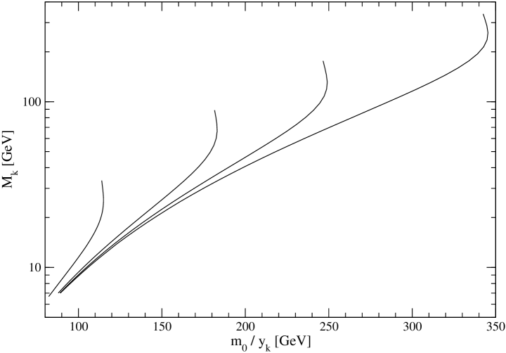
Figure 3: $M_{k}$ versus $m_{0}/y_{k}$ for $y_{k}=0.3,0.5,0.7,1.0$ (left to right) for $\Omega_{d}h^{2}=0.12$, where $y_{k}$ is defined in Eq. (9).

In Figure 3, we plot $M_{k}$ versus $m_{0}/y_{k}$ for $y_{k}=0.3,0.5,0.7,1.0$. As we can see from the figure, the dark matter constraint requires that $M_{k}$ increases as $m_{0}$ increases and for each value of $m_{0}$, it may be as large as $m_{0}$. We also see that $m_{0}/y_{k}$ cannot exceed $350$ GeV or so in the perturbative regime $y_{k}\mathrel{\mathchoice{\vbox{\offinterlineskip\halign{$\m@th\displaystyle\hfil#\hfil$\cr<\crcr\sim\crcr} }}{\vbox{\offinterlineskip\halign{$\m@th\textstyle\hfil#\hfil$\cr<\crcr\sim\crcr} }}{\vbox{\offinterlineskip\halign{$\m@th\scriptstyle\hfil#\hfil$\cr<\crcr\sim\crcr} }}{\vbox{\offinterlineskip\halign{$\m@th\scriptscriptstyle\hfil#\hfil$\cr<\crcr\sim\crcr} }}}1$. This is a very strong constraint, because $m_{0}/y_{k}$ sets the scale also for lepton flavor transitions such as $\mu\to e\gamma$ and the experimental upper bound of its branching fraction cannot be satisfied, unless some cancellation mechanism is at work.

The branching fraction of $\mu\to e\gamma$ is given in this model by [13]

$$B(\mu\to e\gamma)=\frac{3\alpha}{64\pi(G_{F}m_{0}^{2})^{2}}C^{4}\simeq\left(\frac{30~{}\mbox{GeV}}{m_{0}/C}\right)^{4},$$ (13)

where

$$C^{2}=\left|\sum_{i}h_{\mu i}h^{*}_{ei}F_{2}(M_{i}^{2}/m_{0}^{2})\right|,$$ (14)

and

$$F_{2}(x)={1-6x+3x^{2}+2x^{3}-6x^{2}\ln x\over 6(1-x)^{4}}.$$ (15)

Since $M_{k}<m_{0}$ should be satisfied for $N_{k}$ dark matter, the function $F_{2}(x_{k})$ can vary only between $1/12(x_{k}=1)$ and $1/6(x_{k}=0)$. To suppress the branching fraction $B(\mu\to e\gamma)$ which is inversely proportional to the fourth power of $m_{0}$, we need a large value of $m_{0}$. On the other hand, the observed dark matter relic density $\Omega_{d}h^{2}\simeq 0.12$ requires $m_{0}$ to be below 350 GeV for $y_{k}=(\sum_{\alpha\beta}|h_{\alpha k}h_{\beta k}^{*}|^{2})^{1/4}\mathrel{\mathchoice{\vbox{\offinterlineskip\halign{$\m@th\displaystyle\hfil#\hfil$\cr<\crcr\sim\crcr} }}{\vbox{\offinterlineskip\halign{$\m@th\textstyle\hfil#\hfil$\cr<\crcr\sim\crcr} }}{\vbox{\offinterlineskip\halign{$\m@th\scriptstyle\hfil#\hfil$\cr<\crcr\sim\crcr} }}{\vbox{\offinterlineskip\halign{$\m@th\scriptscriptstyle\hfil#\hfil$\cr<\crcr\sim\crcr} }}}1$. This means that if $|\sum_{i}h_{\mu i}h^{*}_{ei}|$ appearing in Eq. (14) is also of order 1, then $B(\mu\to e\gamma)\mathrel{\mathchoice{\vbox{\offinterlineskip\halign{$\m@th\displaystyle\hfil#\hfil$\cr>\crcr\sim\crcr} }}{\vbox{\offinterlineskip\halign{$\m@th\textstyle\hfil#\hfil$\cr>\crcr\sim\crcr} }}{\vbox{\offinterlineskip\halign{$\m@th\scriptstyle\hfil#\hfil$\cr>\crcr\sim\crcr} }}{\vbox{\offinterlineskip\halign{$\m@th\scriptscriptstyle\hfil#\hfil$\cr>\crcr\sim\crcr} }}}5\times 10^{-7}$, which is several orders of magnitude above the experimental upper bound of $1.2\times 10^{-11}$.

To satisfy the $\mu\to e\gamma$ constraint, we consider the possibility that $M_{1,2,3}$ are nearly degenerate. In that limit,

$$({\cal M}_{\nu})_{\alpha\beta}={I(M^{2}/m_{0}^{2})\over M}\sum_{i}h_{\alpha i}h_{\beta i}={\hat{U}}^{*}\pmatrix{m_{1}e^{-i\alpha_{1}}&0&0\cr 0&m_{2}e^{-i\alpha_{2}}&0\cr 0&0&m_{3}}{\hat{U}}^{\dagger},$$ (16)

where ${\hat{U}}$ is given by Eq. (6). A simple solution is then

$$h_{\alpha i}=\left[{Mm_{i}\over I(M^{2}/m_{0}^{2})}\right]^{1/2}~{}e^{-i\alpha_{i}/2}~{}{\hat{U}}_{\alpha i}^{*}~{}\mbox{with}~{}\alpha_{3}=0.$$ (17)

Then we obtain

$$C^{2} = {F_{2}(M^{2}/m_{0}^{2})M\over I(M^{2}/m_{0}^{2})}\left|\sum_{i}{\hat{U}}_{\mu i}{\hat{U}}^{*}_{ei}m_{i}\right|$$ (18)

$$= {F_{2}(M^{2}/m_{0}^{2})M\over I(M^{2}/m_{0}^{2})}\left|{s_{12}c_{12}\over\sqrt{2}}(m_{2}-m_{1})+{s_{13}e^{-i\delta}\over\sqrt{2}}(c_{12}^{2}m_{1}+s_{12}^{2}m_{2}-m_{3})\right|.$$

Thus the suppression of $C^{2}$ is possible because $m_{2}-m_{1}$ is related to $\Delta m^{2}_{sol}$ and $c_{12}^{2}m_{1}+s_{12}^{2}m_{2}-m_{3}$ is related to $\Delta m^{2}_{atm}$ in neutrino oscillations [13, 14].

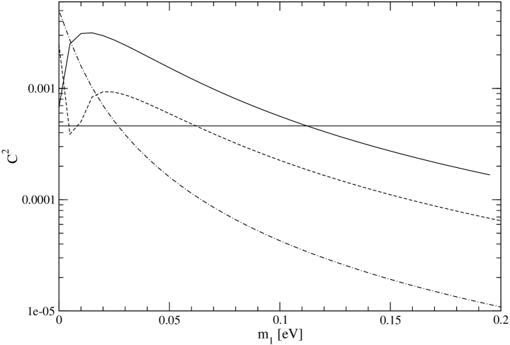
Figure 4: $C^{2}$ versus $m_{1}$ in the case of normal ordering for $s_{13}=0.1~{}(\mbox{solid}),0.05~{}(\mbox{dash}),0.01~{}(\mbox{dot-dash})$, where $C^{2}=4.6\times 10^{-4}$ (horizontal line) corresponds to the experimental upper bound $B(\mu\to e\gamma)=1.2\times 10^{-11}$.

Let us assume $\delta=0$ and consider the normal ordering of neutrino masses, i.e. $m_{3}$ is the largest mass. We then set $h_{3}=\left(\sum_{\alpha}|h_{\alpha 3}|^{2}\right)^{1/2}=1$ which is equivalent to having $Mm_{3}/I(M^{2}/m_{0}^{2})=1$. Hence

$$C^{2}\simeq\left({0.067\over m_{3}}\right)|c_{12}(s_{12}-s_{13}c_{12})(m_{2}-m_{1})-s_{13}(m_{3}-m_{2})|<4.6\times 10^{-4},$$ (19)

where $F_{2}=0.0948$ (corresponding to $m_{0}=345$ GeV and $M=290$ GeV). Using $\Delta m^{2}_{21}=\Delta m^{2}_{sol}=7.9\times 10^{-5}$ eV² and $\Delta m_{32}^{2}=\Delta m^{2}_{atm}=2.3\times 10^{-3}$ eV², we plot $C^{2}$ versus $m_{1}$ in Figure 4 for $s_{13}=0.1,0.05,0.01$. The horizontal line is the experimental bound $C^{2}=4.6\times 10^{-4}$ corresponding to $B(\mu\to e\gamma)=1.2\times 10^{-11}$. We find that for $s_{13}\mathrel{\mathchoice{\vbox{\offinterlineskip\halign{$\m@th\displaystyle\hfil#\hfil$\cr>\crcr\sim\crcr} }}{\vbox{\offinterlineskip\halign{$\m@th\textstyle\hfil#\hfil$\cr>\crcr\sim\crcr} }}{\vbox{\offinterlineskip\halign{$\m@th\scriptstyle\hfil#\hfil$\cr>\crcr\sim\crcr} }}{\vbox{\offinterlineskip\halign{$\m@th\scriptscriptstyle\hfil#\hfil$\cr>\crcr\sim\crcr} }}}0.26$, this constraint cannot be satisfied. For $s_{13}$ less than its experimental bound of $0.2$, there is a lower bound on $m_{1}$ according to the approximate empirical formula

$$\left[{m_{1}\over{\rm eV}}\right]\mathrel{\mathchoice{\vbox{\offinterlineskip\halign{$\m@th\displaystyle\hfil#\hfil$\cr>\crcr\sim\crcr} }}{\vbox{\offinterlineskip\halign{$\m@th\textstyle\hfil#\hfil$\cr>\crcr\sim\crcr} }}{\vbox{\offinterlineskip\halign{$\m@th\scriptstyle\hfil#\hfil$\cr>\crcr\sim\crcr} }}{\vbox{\offinterlineskip\halign{$\m@th\scriptscriptstyle\hfil#\hfil$\cr>\crcr\sim\crcr} }}}0.02+1.4|s_{13}-0.02|-2.9|s_{13}-0.02|^{2},$$ (28)

except for a tiny region near $m_{1}=0$ and $s_{13}=0.09$, and a small region near $m_{1}=0.01$ eV and $s_{13}=0.04$. In Figure 4, we can see that the plot for $s_{13}=0.1$ is getting close to the first region from its dip at $m_{1}=0$, and that the plot for $s_{13}=0.05$ has a small allowed range near $m_{1}=0.01$ eV.

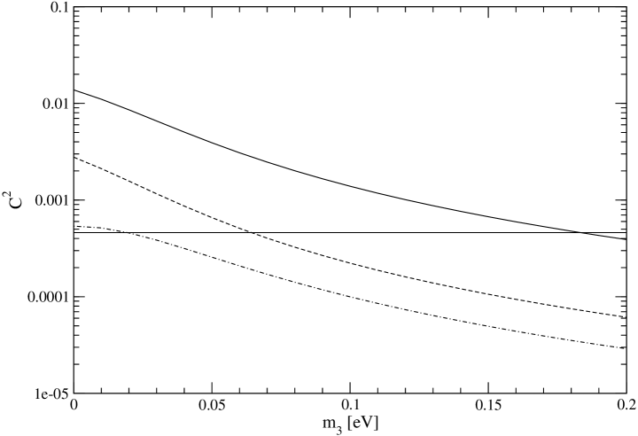
Figure 5: $C^{2}$ versus $m_{3}$ in the case of inverted ordering for $s_{13}=0.2~{}(\mbox{solid}),-0.05~{}(\mbox{dash}),0.0~{}(\mbox{dot-dash})$.

In the case of inverted ordering, i.e. $m_{2}$ is the largest mass, we are already guaranteed that $m_{1,2}>\sqrt{\Delta m^{2}_{32}}\simeq 0.048$ eV. For completeness, we set $h_{2}=1$ and plot $C^{2}$ versus $m_{3}$ in Figure 5 for $s_{13}=0.2,-0.05,0.0$. Here, for $s_{13}\mathrel{\mathchoice{\vbox{\offinterlineskip\halign{$\m@th\displaystyle\hfil#\hfil$\cr>\crcr\sim\crcr} }}{\vbox{\offinterlineskip\halign{$\m@th\textstyle\hfil#\hfil$\cr>\crcr\sim\crcr} }}{\vbox{\offinterlineskip\halign{$\m@th\scriptstyle\hfil#\hfil$\cr>\crcr\sim\crcr} }}{\vbox{\offinterlineskip\halign{$\m@th\scriptscriptstyle\hfil#\hfil$\cr>\crcr\sim\crcr} }}}0.24$ and $s_{13}\mathrel{\mathchoice{\vbox{\offinterlineskip\halign{$\m@th\displaystyle\hfil#\hfil$\cr<\crcr\sim\crcr} }}{\vbox{\offinterlineskip\halign{$\m@th\textstyle\hfil#\hfil$\cr<\crcr\sim\crcr} }}{\vbox{\offinterlineskip\halign{$\m@th\scriptstyle\hfil#\hfil$\cr<\crcr\sim\crcr} }}{\vbox{\offinterlineskip\halign{$\m@th\scriptscriptstyle\hfil#\hfil$\cr<\crcr\sim\crcr} }}}-0.27$, the experimental constraint cannot be satisfied. In other words, the constraint on $\theta_{13}$ from $\mu\to e\gamma$ coincides roughly also with that from neutrino oscillations.

For the simple solution of Eq. (16), as we can see from Figure 4 and 5, all the neutrino masses may be assumed to be degenerate to satisfy the $\mu\to e\gamma$ constraint; hence the effective mass $\langle m_{ee}\rangle$ in neutrinoless double beta decay is approximately given by

$$\langle m_{ee}\rangle\simeq m_{1}|0.572+0.428\cos(\alpha_{1}-\alpha_{2})|^{1/2}.$$ (29)

We also allow the heavy $N_{i}$ masses $M_{1,2,3}$ to be slightly different, so that our approximation that only one of them is the candidate for dark matter remains valid. Note that $\Delta M/M$ only needs to be of order $10^{-3}$ for Eq. (18) to be valid. In analogy to $\mu\to e\gamma$, there are also dark-matter contributions to $\tau\to\mu\gamma$, $\tau\to e\gamma$, and the anomalous magnetic moment of the muon. However, they are at least one or more orders of magnitude below the present experimental bounds.

In conclusion, we have shown how cold dark matter and neutrinoless double beta decay may be connected if neutrinos acquire mass only because of their interactions with dark matter. We repeat the basic argument presented earlier. The existence of dark matter requires a class of new particles which are odd with respect to an exactly conserved $Z_{2}$ symmetry. Their interactions with neutrinos and charged leptons must not be too weak to be identified as cold dark matter with the correct value of their relic density in the Universe at present. On the other hand, they are also responsible for the masses of neutrinos and their observed mixing in neutrino oscillations. This implies necessarily flavor changing transitions such as $\mu\to e\gamma$. In order to suppress the latter, the parameter space of neutrino masses is limited, thereby enforcing a lower bound on neutrinoless double beta decay. For $N$ as dark matter, this is typically of order 0.05 eV, even though much lower values are still allowed from accidental cancellations. More importantly, this connection between cold dark matter and neutrinoless double beta decay can be tested in the near future at the Large Hadron Collider and complemented by a host of experiments on neutrino oscillations and neutrinoless double beta decay already under way and being planned.

This work was supported in part by the U. S. Department of Energy under Grant No. DE-FG03-94ER40837. We thank Haruhiko Terao for valuable discussions. EM also thanks the Institute for Theoretical Physics, Kanazawa University for hospitality during a recent visit.

References

[1] For a recent review, see for example G. Bertone,
D. Hooper, and J. Silk, Phys. Rept. 405, 279 (2005).
[2] E. Ma, Phys. Lett. B625, 76 (2005).
[3] R. Barbieri, L. J. Hall, and V. S. Rychkov,
hep-ph/0603188.
[4] S. Weinberg, Phys. Rev. Lett. 43, 1566 (1979).
[5] E. Ma, Phys. Rev. Lett. 81, 1171 (1998).
[6] M. Gell-Mann, P. Ramond, and R. Slansky, in
Supergravity, eds. P. van Nieuwenhuizen and D. Z. Freedman
(North-Holland, 1979), p. 315; T. Yanagida,
in Proc. of the Workshop on
the Unified Theory and the Baryon Number in the Universe,
eds. O. Sawada and
A. Sugamoto, KEK Report No. 79-18 (Tsukuba, Japan, 1979),
p. 95; R. N. Mohapatra and G. Senjanovic,
Phys. Rev. Lett. 44, 912 (1980).
[7] L. M. Krauss, S. Nasri, and M. Trodden, Phys. Rev. D67,
085002 (2003).
[8] E. Ma, Phys. Rev. D73, 077301 (2006).
[9]
D. N. Spergel et al.,
WMAP Collaboration, Astrophys. J. Suppl. 148, 175 (2003).
[10]
M. Tegmark et al., SDSS Collaboration,
Phys. Rev. D69, 103501 (2004).
[11]
K. Griest, Phys. Rev. D38, 2357 (1988).
[12]
K. Griest, M. Kamionkowski, and M. S. Turner,
Phys. Rev. D41, 3565 (1990).
[13] E. Ma and M. Raidal, Phys. Rev. Lett. 87,
011802 (2001).