X

The Minimal Set of
Electroweak Precision Parameters

G. Cacciapaglia^a, C. Csáki^a, G. Marandella^b, and A. Strumia^c

^a Institute for High Energy Phenomenology
Newman Laboratory of Elementary Particle Physics
Cornell University, Ithaca, NY, 14853, USA
^b Department of Physics, University of California, Davis, CA 95616, USA
^c Dipartimento di Fisica dell’Università di Pisa and INFN, Italia

Abstract

We present a simple method for analyzing the impact of precision electroweak data above and below the $Z$-peak on flavour-conserving heavy new physics. We find that experiments have probed about ten combinations of new physics effects, which to a good approximation can be condensed into the effective oblique parameters $\hat{S},\hat{T},\hat{U},V,X,W,Y$ (we prove positivity constraints $W,Y\geq 0$) and three combinations of quark couplings (including a distinct parameter for the bottom). We apply our method to generic extra $Z^{\prime}$ vectors.

1 Introduction

The successes of the Standard Model (SM) became so boring that various physicists wonder if they contain an important message: the lack of evidence for new physics pushes many proposed solutions of the higgs mass hierarchy problem into more-or-less unnatural corners of their parameter space.

Global fits do not provide much intuition into the origin of the strongest constraints, or even on the number of new-physics parameters that are strongly constrained. Here we present an efficient and simple general analysis of electroweak precision data using an effective-theory description. Assuming that new physics is somewhat above the weak scale, its low-energy effects can be described by an effective Lagrangian that contains leading non-renormalizable terms. Even assuming that the new physics is generation independent (i.e. no new flavour physics), previous analyses identified an irreducible set of 10 gauge-invariant operators [1] contributing to precision measurements at and below the $Z$-pole. This list of operators has grown to about 20 [2], after that the relevance of LEP2 precision measurements above the $Z$-pole was pointed out [3].

We here show that experiments have so far precisely probed only about 10 combinations of the 20 operators. However, if one follows the traditional route of constraining new physics one must compute all operators and then perform a global fit to all 20 parameters: otherwise one cannot know if the new physics corresponds to a strongly or weakly constrained combination of higher dimensional operators.

The main aim of this paper is to develop a simpler strategy: we identify a minimal set of parameters that are strongly constrained, extending the $Z$-pole parameters of [4]. In this way, cancellations between the various operators, like the ones pointed out in [5], are already built-in to this formalism. The data requires almost all of these parameters to be compatible with the SM at the per mille level. Moreover, we want our minimal set to catch the main features of the measurements: a reasonably accurate bound on the scale of new physics can be extracted by just considering our minimal set of parameters and without the necessity of a complete analysis.

We start by identifying the sub-set of most precise measurements, mostly performed at $e^{+}e^{-}$ colliders (LEP1, LEP2, SLD). Those experiments studied all $f\bar{f}$ final states, but could measure leptonic final states more precisely than hadronic final states. We will show that the corrections to all leptonic data can be converted into oblique corrections to the vector boson propagators, and condensed into the seven parameters $\hat{S}$, $\hat{T}$, $W$, $Y$, $X$, $\hat{U}$ and $V$ defined in [3]. (Unlike in [3] we do not restrict our attention to oblique new physics). Indeed, starting with a generic set of higher-dimensional operators, one can use the three equations of motion for $W^{+},Z,\gamma$ to eliminate the three currents involving charged leptons from the higher dimensional operators:

$$\bar{e}_{L}\gamma_{\mu}e_{L},\qquad\bar{e}_{R}\gamma_{\mu}e_{R},\qquad\bar{e}_{L}\gamma_{\mu}\nu_{L}+\hbox{h.c.}\,.$$ (1.1)

Parameterizing the new physics in terms of corrections to vector boson propagators is convenient because: i) in many models the oblique parameters can be calculated directly [7, 3, 6], without having to first calculate the general set of induced higher dimensional operators; ii) it is also easier to compute how the observables are affected by oblique corrections; iii) it allows one to unambiguously identify the most relevant corrections to electroweak precision measurements in any generic model.

We will show that already this subset of parameters is enough to establish the correct bound on generic models within a ‘typical’ 20% accuracy. Thus for most models it suffices to calculate the seven generalized oblique parameters to establish a reasonably accurate bound on the scale of new physics, with the caveat that the approximation fails spectacularly if, for some reason, new physics is leptophobic (i.e. if quarks are much more strongly affected than leptons).

A more accurate approximation is obtained by adding more parameters in the quark sector. Basically, we keep the oblique approximation in the ${\rm U}(1)_{Y}$ sector but not in the ${\rm SU}(2)_{L}$ sector. In practice, this amounts to adding 2 more parameters that describe the coupling of the left-handed quarks (which is better measured because the larger SM coupling to the $Z$ enhances the interference term with respect to the right-handed components). Finally, we allow the third-generation of quarks to behave differently from lighter quarks, and describe this possibility by adding one extra parameter: the traditional $\varepsilon_{b}$ [8]. This choice is motivated by theoretical considerations (in many models of electroweak symmetry breaking the top sector is special), by experimental considerations ($b$-tagging allows to probe $b$-quarks more precisely than lighter quarks) and by phenomenological considerations (flavor universality can be significantly violated only in the third generation).

We finally present numerical fits for our $7+2+1$ new-physics parameters,

$$\hat{S},\hat{T},\hat{U},V,X,W,Y,C_{q},\delta\varepsilon_{q},\delta\varepsilon_{b}$$

emphasizing their combinations that are most strongly constrained. Furthermore, in section 5 we show that first principles imply positivity constraints on $W,Y\geq 0$.

The paper is organized as follows: in section 2 we introduce our formalism and identify the relevant parameters. In section 3 we fit these parameters and compare the results with the complete analysis, showing how accurate our approximation typically is. In sec 4 we apply the formalism to the specific case of various extra $Z^{\prime}$ bosons, compiling present constraints. In section 5 we demonstrate the positivity constraint on the oblique parameters $W$ and $Y$. In the appendix, we explicitly write the relation between our parameters and a general basis of gauge-invariant operators.

2 The minimal set of constrained parameters

The effects of heavy new physics on precision electroweak observables can be described by adding to the SM Lagrangian dimension 6 operators that depend on the SM fields: the gauge bosons $W^{\pm}$, $Z$ and the photon $A$, the Higgs vev $v$, the fermionic currents $J_{ff^{\prime}}=\bar{f}\gamma^{\mu}f^{\prime}$, and their derivatives:

$$\mathscr{L}_{\rm BSM}\,\big{(}W^{\pm}_{\mu},Z_{\mu},A_{\mu},\partial_{\mu},v,J_{ff^{\prime}}\big{)}\,.$$ (2.1)

We are interested here in terms that do not violate flavor and CP (and, of course, electric charge and color should also be conserved). The electroweak gauge symmetry ${\rm SU}(2)_{L}\otimes{\rm U}(1)_{Y}$, spontaneously broken by the Higgs vev, implies some relations among the coefficients of the dimension-6 terms. There are many such operators [9]. After eliminating the operators that do not affect precision data and the operators that on-shell are equivalent to combinations of other operators, one still has to deal with many operators: 10 if LEP2 is not included [1], and, including LEP2, 20 operators were considered in [2]. In agreement with [5] (where it was pointed out that two combinations can be expressed in terms of unconstrained operators) we find that precision data are affected by 18 independent operators, listed in Appendix A.

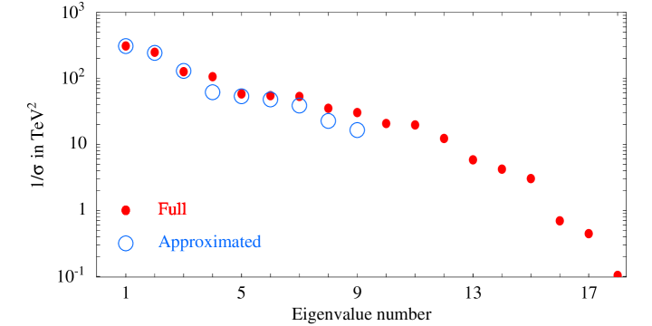
Figure 1: The red dots are the ordered eigenvalues of the full error matrix, that describe the sensitivity of present data (upper dots correspond to more precise combinations). Precision data significantly constrain only about 10 new-physics effects. The blue circles show the same eigenvalues recomputed making our simplifying approximation.

In practice, however, many combinations of different operators are poorly constrained. A global analysis contains this information: one can obtain electroweak precision bounds on a model by computing all induced higher dimensional operators. Our aim is to simplify this program by finding the suitable variables where possible cancellations are manifest, and drop the unnecessary information.

In order to find the number of parameters that are strongly constrained by the electroweak precision data we first perform the traditional global analysis including all relevant higher dimensional operators. In Fig. 1 we plot the eigenvalues of the error matrix, computed in the uniformly-normalized basis described in Appendix A. This automatically identifies all correlations of theoretical, experimental and accidental nature. For example: i) if one measurement constrains one combination of many operators, it will appear here as one constraint; ii) if a combination of operators does not affect any observable, it will appear here as a zero eigenvalue. Fig. 1 shows that precision data really constrain about 10 new-physics effects, and that a few constraints often dominate the global fit. We want to find a simple physically motivated basis for the electroweak parameters that automatically separates the strongly constrained combinations from the weakly constrained ones.

We will therefore use a different approach: once a specific set of higher dimensional operators of the form (2.1) is given, we can use the equations of motion of the 3 gauge bosons $W^{\pm},Z,\gamma$ to eliminate 3 fermionic currents: we choose to eliminate the currents involving charged leptons listed in eq. (1.1). The reason is that most of the precision measurements have been perfomed at $e^{+}e^{-}$ colliders (LEP1, LEP2 and SLD), strongly constraining operators involving charged leptons. Neutrinos on the other hand are experimentally more difficult to deal with than charged leptons. This is the reason why we have chosen to use the equations of motion in a way that is not explicitly ${\rm SU}(2)_{L}$ invariant. Muon-decay, which gives the most precise test of neutrino couplings, is fully described by oblique couplings because it involves charged currents and we eliminated all new physics involving the $\bar{e}_{L}\gamma_{\mu}\nu_{L}$ current.

In our formalism, the most general effective Lagrangian describing new physics can be split into two parts:

$$\mathscr{L}_{\rm BSM}=\mathscr{L}_{\rm oblique}+\mathscr{L}_{\rm couplings}+\dots$$ (2.2)

where the dots stand for terms that do not affect precision measurements. Note again that, due to our choice for the use of the equations of motion, $\mathscr{L}_{\rm couplings}$ will not contain any currents involving the charged leptons. Therefore the oblique terms in $\mathscr{L}_{\rm oblique}$ fully encode corrections to the most precisely measured precision observables involving charged lepton final states:

$$\alpha_{\rm em},~{}\Gamma(\mu),~{}M_{Z},~{}M_{W},~{}\Gamma(Z\to\ell\bar{\ell}),~{}A^{\ell}_{FB},~{}A^{\ell}_{LR},~{}A_{\rm pol}^{\tau},~{}\sigma_{\rm LEP2}(e\bar{e}\to\ell\bar{\ell}),~{}ee\to ee.$$

$\mathscr{L}_{\rm couplings}$, on the other hand, contains corrections to the couplings of quark and neutrino currents: it affects observables involving neutrinos and quarks :

$$\Gamma(Z\to\nu\bar{\nu}),~{}\Gamma(Z\to q\bar{q}),~{}A^{b}_{FB},~{}A^{b}_{LR},~{}A^{c}_{LR},~{}A^{c}_{FB},\sigma_{\rm LEP2}(e\bar{e}\to q\bar{q}),~{}Q_{W}\,.$$

This formalism therefore allows one to clearly distinguish which parameters are more constrained than others. This approach has already been used in the case of models with universal new physics [3] (e.g. gauge bosons in extra dimensions, most little Higgs models [12], Higgsless models [13]), where all corrections involving fermions only appear in combinations proportional to SM gauge currents. As a consequence, all fermion operators can be completely transformed into oblique operators by using the equations of motion for vectors. More importantly, in various concrete models one can bypass the step of identifying the set of induced dimension six operators: by integrating out the combinations of new-physics vectors not coupled to fermions (rather than the heavy mass eigenstates) directly gives the Lagrangian in terms of the oblique parameters. Thus this method simplifies both the intermediate computations and the final result. Here we show that this formalism is also useful in the case of generic non-universal models (e.g. fermions that live in different places in extra dimensions, some Little Higgs models [14], models with extra $Z^{\prime}$ bosons).

In the next part of this section, we review the standard parametrization of oblique new physics. We later present the generic form for $\mathscr{L}_{\rm couplings}$, emphasizing the (weak) restrictions imposed by ${\rm SU}(2)_{L}$-invariance, and discuss to which extent $\mathscr{L}_{\rm couplings}$ can be neglected. In Appendix A we also explicitly show how the equations of motion allow us to relate the standard basis of ${\rm SU}(2)_{L}$-invariant dimension 6 operators to our parametrization. These operators are assumed to have generic coefficients, such that Appendix A applies to generic new physics. More importantly, in section 4 we show, in a specific example of new physics (a heavy $Z^{\prime}$), how one can directly compute the full set of oblique parameters without having to pass trough the standard basis.

2.1 The oblique parameters

Here we review how generic heavy new physics can affect the kinetic terms of vector bosons, $\Pi_{33}(p^{2})$, $\Pi_{30}(p^{2})$, $\Pi_{30}(p^{2})$, $\Pi_{WW}(p^{2})$, defined by the effective Lagrangian

$$\mathscr{L}_{\rm oblique}=-\frac{1}{2}W^{3}_{\mu}\Pi_{33}(p^{2})W^{3\mu}-\frac{1}{2}B_{\mu}\Pi_{00}(p^{2})B^{\mu}-W^{3}_{\mu}\Pi_{30}(p^{2})B^{\mu}-W_{\mu}^{+}\Pi_{WW}(p^{2})W^{\mu}_{-}\,.$$ (2.3)

Since new physics is assumed to be heavy, we can expand the $\Pi$’s in powers of $p^{2}$:

$$\Pi(p^{2})=\Pi(0)+p^{2}\,\Pi^{\prime}(0)+\frac{(p^{2})^{2}}{2}\,\Pi^{\prime\prime}(0)+\dots$$ (2.4)

neglecting higher order terms, that for dimensional reasons correspond to operators of dimension higher than 6. This expansion contains 12 parameters: 3 can be reabsorbed in the definitions of the SM parameters $g$, $g^{\prime}$ and $v$ and 2 vanish because of electro-magnetic gauge invariance: the photon is massless and couples to $Q=T_{3}+Y$. New physics is described by 7 dimensionless oblique parameters, defined as (contrary to [3] we use canonically normalized kinetic terms)

$$\begin{array}[]{c}\displaystyle\hat{S}=\frac{g}{g^{\prime}}\Pi_{30}^{\prime}\,,\quad\hat{T}=\frac{\Pi_{33}-\Pi_{WW}}{M_{W}^{2}}\,,\quad W=\frac{M_{W}^{2}}{2}\;\Pi^{\prime\prime}_{33}\,,\quad Y=\frac{M_{W}^{2}}{2}\;\Pi^{\prime\prime}_{00}\,,\\ \displaystyle\hat{U}=\Pi^{\prime}_{WW}-\Pi^{\prime}_{33}\,,\qquad V=\frac{M_{W}^{2}}{2}\;(\Pi^{\prime\prime}_{33}-\Pi^{\prime\prime}_{WW})\,,\qquad X=\frac{M_{W}^{2}}{2}\;\Pi^{\prime\prime}_{30}\,,\end{array}$$ (2.5)

where all $\Pi$’s are computed at $p^{2}=0$. These parameters correct the propagators of the gauge bosons, affecting the precision observables. Only 6 combinations actually enter observables involving charged leptons: in particular, only the combination $\hat{U}-V$. $Z$-pole precision data can be encoded in the $\varepsilon$’s of [15]. Low energy data do not depend on $\hat{U},V$. The $e\bar{e}\to f\bar{f}$ cross sections measured at LEP2 are dominantly affected by $Y$, $W$ and $X$ [3].

Using ${\rm SU}(2)_{L}$-invariance one can show that $V\ll\hat{U}\ll\hat{T}$ and $X\ll\hat{S}$: in the case of universal new physics, the sub-leading form factors $\hat{U},V,X$ can therefore be neglected and new physics is fully described by $\hat{S},\hat{T},W,Y$ [3]. This argument however does not apply in our case, where the same parameters are applied in a different context: to describe how generic heavy new physics (not necessarily universal) affects observables that only involve charged leptons and vectors. To reach the basis in which charged-leptonic data are condensed into vector propagators we made a transformation which is not ${\rm SU}(2)_{L}$-invariant. As a consequence all oblique parameters generically arise at leading order.

2.2 Vertex corrections

Here we present the effective Lagrangian that describes new-physics corrections to $Z,\gamma$ couplings, taking into account a) that we eliminated currents involving charged leptons; b) that new physics is heavy, allowing a low-energy expansion in momenta; c) electromagnetic gauge invariance. A convenient parametrization is:

$$\mathscr{L}_{\rm couplings}=\sum_{f}(\bar{f}\gamma^{\mu}f)\left[e\,A_{\mu}\,\frac{C^{\gamma}_{f}}{M_{W}^{2}}\,p^{2}+\sqrt{g^{2}+{g^{\prime}}^{2}}\,Z_{\mu}\left(\frac{C^{Z}_{f}}{M_{W}^{2}}\,(p^{2}-M_{Z}^{2})+\delta g_{f}\right)\right]\,,$$ (2.6)

where $f={u_{L},d_{L},u_{R},d_{R},\nu_{L}}$, and higher orders in the momentum again correspond to subleading effects due to operators with dimensions greater than 6. The $\delta g$’s are corrections to on-shell $Z$ couplings, tested by measurements at the $Z$-pole. The $C^{\gamma}$ and $C^{Z}$ are equivalent to 4-fermion contributions to $e^{+}e^{-}\rightarrow q\bar{q}$: the $p$-dependence cancels the propagator of the gauge boson, and we are left with a constant ($p$-independent) contribution. They affect LEP2, atomic parity violation, etc. For the neutrinos only $\delta g_{\nu_{L}}$ is measured via the invisible decay ratio of the $Z$.

${\rm SU}(2)_{L}$ invariance implies some mild restrictions on these vertex parameters:

1. As shown in Appendix A, $\delta g_{L\nu}$ is fixed in terms of oblique parameters as:

   $$\delta g_{L\nu}=V-\frac{1}{2}\hat{U}-\tan\theta_{W}X\,.$$ (2.7)

   Notice that it depends on a different combination of $\hat{U}$ and $V$ than the one entering corrections to the gauge boson propagators. This means that considering all the 7 oblique parameters defined in the previous subsection is enough to include the relevant neutrino measurements.

2. In the quark sector we apparently have 12 new parameters: $\delta g_{L,R\,u,d}$ and $C^{Z,\gamma}_{L,R\,u,d}$. However only 11 of them are independent, and correspond to the 11 quark operators of [2]. Indeed, as explicitly shown in Appendix A, the following relation holds between the 4-fermion coefficients of the left-handed quarks:

   $$(C^{\gamma}_{dL}-C^{\gamma}_{uL})=\cos^{2}\theta_{W}(C^{Z}_{dL}-C^{Z}_{uL})+\frac{X}{\tan\theta_{W}}.$$ (2.8)

2.3 A simple approximation

We can now proceed with the final counting. We have 18 independent coefficients: the 7 oblique parameters $\hat{S},\hat{T},\hat{U},V,X,Y,W$, 4 $\delta g$’s for the quarks, 4 quark $C^{Z}_{q}$’s and 3 independent $C^{\gamma}_{q}$’s. The counting agrees with the results of [5], that shows how 2 combinations of the 21 operators of [2] can be eliminated. (18 arises as $21-2-1$: one further operator, that only affects $e^{-}e^{+}\to W^{+}W^{-}$, is ignored here because we do not view this as a ‘precision’ measurement. This view is corroborated by the numerical results of [2, 5].) In other words, the unconstrained combinations pointed out in [5] are automatically eliminated in our formalism.

Our basis makes a clear separation of which parameters contribute to which measurements. Corrections to observables involving leptons only are expressed in terms of the seven oblique parameters (which as we have seen also include neutrinos). Observables involving quarks in the final state at the $Z$-pole involve in addition only the four $\delta g$’s. The $C^{\gamma,Z}_{q}$’s are only necessary for $\sigma(e\bar{e}\to q\bar{q})$ at LEP2 and atomic parity violation.

As leptonic final states are generically better measured than hadronic ones, this separation already suggests that describing the precision measurements in terms of only the 7 oblique parameters could be a reasonable approximation (oblique approximation). In the next section we will check numerically that this indeed happens. This approximation also includes the constraints on neutrinos.

In order to be more accurate, we want to add a minimal set of parameters describing corrections in the hadronic sector. In fact, not all the quark observables are well measured, so that only a small subset of parameters will actually contribute most strongly to the bound. At the $Z$-pole, the better measured quantity is the hadronic branching ratio of the $Z$. It depends on the combination:

$$g^{\rm SM}_{qL}\,\delta g_{qL}+g^{\rm SM}_{qR}\,\delta g_{qR}\,.$$

Due to the fact that the couplings of the right-handed components to the $Z$ are generically smaller than the couplings of the left-handed component (by a factor of 0.18 for the down type quarks, and 0.44 for the up type), we expect in general that only the corrections involving left-handed quarks will be relevant. Moreover, when the contribution of up and down quarks are summed, the result is proportional to:

$$\delta g_{uL}-\delta g_{dL}-\frac{\tan^{2}\theta_{W}}{3}\,(\delta g_{uL}+\delta g_{dL})\,,$$

so that the difference between the two parameters seems to be more relevant than the sum.

Similar arguments apply for the hadronic cross section measured at LEP2. The main difference is the presence of interference with the SM diagram with a photon exchange, and the presence of 4-fermion operators. We first notice that the interference with the photon is generically suppressed by the gauge coupling $e$ versus $\sqrt{g^{2}+{g^{\prime}}^{2}}$: this results in a suppression of order $\sin\theta_{W}$. The contribution of the $\delta g$’s will therefore enter in the same way as in the hadronic branching ratio. A very similar argument can be applied to the 4-fermion contribution, so that only the combinations $C^{Z}_{Lu}-C^{Z}_{Ld}$ and $C^{\gamma}_{Lu}-C^{\gamma}_{Ld}$ are constrained: as already mentioned in (2.8) these two parameters are related to each other, so that they correspond to a single parameter. From this rough argument we can thus infer that 2 parameters will be most relevant in the quark sector:

$$\halign to=0.0pt{\@eqnsel\hskip\@centering$\displaystyle{#}$&\global\@eqcnt\@ne\hskip 2\arraycolsep\hfil${#}$\hfil& \global\@eqcnt\tw@\hskip 2\arraycolsep$\displaystyle{#}$\hfil&\llap{#}\cr 0.0pt plus 1000.0pt$\displaystyle{\delta\varepsilon_{q} &10.0pt\hfil${= &10.0pt$\displaystyle{\delta g_{uL} - \delta g_{dL}\,, \\ \delta C_{q} &\hbox to0.0pt{\hss= &C^{Z}_{uL}-C^{Z}_{dL}\,.&(2.9)\cr}}}}}$$

Again, in the next section we will numerically show that this is indeed the case.

Until now we have assumed flavor universality including the third generation, and in particular the bottom quark. However, in many models of electroweak symmetry breaking the third generation of quarks is special due to the heavyness of the top quark, and it is differently affected by new physics. For this reason, we will relax the flavor universality for the bottom quark, and deal with it separately. This is also necessary since the bottom final state is well measured. At LEP1, only $\delta g_{bL}$ is well measured, because the SM coupling of the right-handed component is smaller, thus we can define:

$$\delta g_{bL}=-\frac{1}{2}\delta\varepsilon_{b}\,;$$ (2.10)

here the parameter $\delta\varepsilon_{b}$ coincides with the standard definition given in [8]. Notice that the anomalous $A_{FB}^{b}$ measurement gives a subleading contribution to the determination of $\delta\varepsilon_{b}$. The cross section $\sigma(e\bar{e}\to b\bar{b})$ at LEP2 also depends on a combination of 4-fermion operators. In general an extra parameter should also be added to the fit: however, in model of electroweak symmetry breaking involving the top quark, we expect corrections to $\delta\varepsilon_{b}$ to be more important. The reason is that the 4-fermion operators with the bottom will also involve couplings of new physics with the electron, already tightly constrained by the oblique parameters. This is the case, for example, in models with dynamical symmetry breaking [16], gauge-Higgs unification [17] or Higgsless models [13]. Thus, in order to simplify the analysis, we will approximate a flavour-universal contribution to the bottom 4-fermion operators. In this way, only one parameter is sufficient to describe the bottom.

3 Global fit

In this section we study the fit of the precision electroweak measurements, and show that the approximations proposed in the previous section are actually sensible, and give a sufficiently reliable bound on generic models of new physics. One can express all the observables in terms of the following 18 parameters: the 7 oblique parameters $\hat{S}$, $\hat{T}$, $\hat{U}$, $W$, $Y$, $V$ and $X$, 4 corrections to the couplings of the $Z$ with quarks $\delta g_{uR}$, $\delta g_{dR}$, $\delta g_{uL}$, $\delta g_{dL}$, and 7 4-fermion parameters (4 involving right-handed quarks $C^{\gamma}_{uR}$, $C^{\gamma}_{dR}$, $C^{Z}_{uR}$, $C^{Z}_{dR}$, and 3 involving left-handed quarks $C^{Z}_{uL}$, $C^{Z}_{dL}$, and $C^{\gamma}_{uL}+C^{\gamma}_{dL}$). Note that in doing this we are not yet introducing any approximation: we are just choosing a particular basis for the dimension 6 operators affecting electroweak precision observables.

The two approximations we want to pursue are the following: first we consider only the 7 oblique parameters $\hat{S}$, $\hat{T}$, $\hat{U}$, $W$, $Y$, $V$ and $X$ (oblique approximation) and set all the others to zero: this allows us to exactly describe the observables only involving vectors and leptons (charged and neutrinos), but, in general, does not correctly describe corrections to quark observables. Next, as argued in the previous section, in the quark sector two parameters should have the strongest effect on the bound on new physics. They are related to corrections to the couplings to the $Z$ and 4-fermion operators involving left-handed components, $\delta\varepsilon_{q}$ and $\delta C_{q}$.

We now check how good our approximations are for guessing the bound on the scale $\Lambda$ of new physics in generic models. To do that, we generated many random models by writing each parameter as $r/\Lambda^{2}$, where $-1\leq r\leq 1$ are random numbers. This is an reasonably arbitrary procedure. We then extract the bound on $\Lambda$ both from the exact fit and the approximate fits. The result is graphically shown in Fig. 2: in case (a) we show the oblique approximation; in (b) we add the two parameters $\delta C_{q}$ and $\delta\varepsilon_{q}$ for the quarks to the oblique parameters; in (c) we include all the parameters except $\delta C_{q}$ and $\delta\varepsilon_{q}$. In the following table we report, for the same cases, the average value and the variance of $\Lambda_{\rm approx}/\Lambda_{\rm true}$.

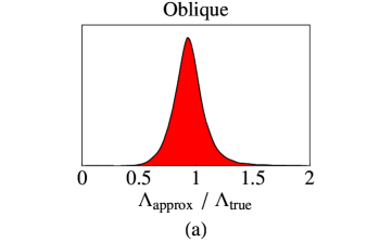
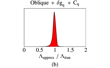
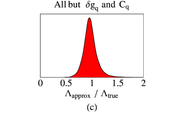
Figure 2: Distibutions of the ratios between the approximate over true bound in various approximations. In the first “oblique” panel we include in the fit only $\hat{S}$, $\hat{T}$, $\hat{U}$, $W$, $Y$, $V$ and $X$. In the second panel we add the two parameters $\delta C_{q}$ and $\delta\varepsilon_{q}$ for the quarks. Finally we include all the parameters except $\delta C_{q}$ and $\delta\varepsilon_{q}$.

Approximation	$\Lambda_{\rm approx}/\Lambda_{\rm true}$
Oblique	$0.95\pm 0.16$
Oblique plus $C_{q}$, $\delta\varepsilon_{q}$	$0.98\pm 0.06$
All but $C_{q}$, $\delta\varepsilon_{q}$	$0.98\pm 0.15$

We see that the oblique approximation is already reasonable: in most of the cases the approximate bound is less than $25\%$ away from the correct one. Adding the two parameters $\delta C_{q},\delta\varepsilon_{q}$ improves the approximation significantly: in more than $90\%$ of the cases the approximate bound reproduces the exact one within $10\%$. Furthermore, it is important to notice that considering a fit where all the parameters except $\delta C_{q},\delta\varepsilon_{q}$ are added does not improve much the approximation with respect to the oblique case. This is telling us that in the quark sector it is indeed $\delta C_{q}$ and $\delta\varepsilon_{q}$ which are the most constrained parameters, while all the others are much less constrained (and mostly negligible for establishing a reliable bound on the scale of new physics). The arguments we have discussed in section 2.2 thus find a quantitative verification here. Out of the 18 initial parameters only 9 are truly constrained. The remaining 9 can be safely neglected.

Fig. 1 compares the eigenvalues of the full error matrix with the eigenvalues recomputed using our simplified approximation (using of course the same normalization in the two cases). We see that the approximation catches the main constraints, ignoring the remaining weakly constrained combinations. We do not show the full eigenvalues extracted from the global fit of [2], that show a similar level of agreement.

We now present how data determine our 10 parameters by presenting the ‘eigenvectors’ of the global $\chi^{2}$, i.e. we show the orthogonal combinations that have been determined with no statistical correlation with the other combinations, such that a model is excluded if any one of these combinations contradicts experimental data. We order them starting from the most precise ones. They are:

$$R\cdot\left(\begin{array}[]{c}\hat{S}\\ \hat{T}\\ \hat{U}\\ V\\ W\\ X\\ Y\\ \delta C_{q}\\ \delta\varepsilon_{b}\\ \delta\varepsilon_{q}\end{array}\right)=10^{-3}\left(\begin{array}[]{c}-0.04+0.54\ell\pm 0.21\\ +0.13+0.08\ell\pm 0.43\\ +0.41+0.21\ell\pm 0.50\\ +0.16+0.72\ell\pm 0.54\\ -0.36-0.33\ell\pm 0.75\\ 0+0.16\ell\pm 1.2\\ -0.9-0.12\ell\pm 1.5\\ -5.6-0.31\ell\pm 2.0\\ -0.4+0.18\ell\pm 8.7\\ -26+0.66\ell\pm 18\end{array}\right)$$ (3.21)

where the factor $\ell=\ln(m_{h}/M_{Z})$ encodes the approximate dependence on the Higgs mass and the orthogonal matrix $R$ equals

$$R=10^{-3}\left(\begin{array}[]{cccccccccc}-404&353&-133&173&137&-753&276&4&18&27\\ -245&-19&492&-747&30&-37&280&15&-40&-235\\ -16&208&146&-152&-724&-224&-407&319&33&260\\ -222&691&-76&5&-120&550&285&-129&55&216\\ -17&-330&177&-36&114&-31&273&-12&1&876\\ 3&232&-7&-283&303&-118&-589&-581&-175&209\\ -42&-68&132&31&-44&-37&-66&-288&939&-33\\ -203&-200&350&375&-445&-9&126&-587&-282&-124\\ -642&-381&-575&-219&-161&147&-112&-41&9&11\\ 519&0&-458&-341&-329&-199&376&-337&-1&2\end{array}\right).$$

The two last combinations have large uncertainties and can be ignored. The flavour-universal limit is obtained by setting $\delta\varepsilon_{b}=\delta\varepsilon_{q}$.

4 Example: a generic $Z^{\prime}$

We now apply our results to a specific concrete example: a generic heavy non-universal $Z^{\prime}$ vector boson, with mass $M_{Z^{\prime}}$, gauge coupling $g_{Z^{\prime}}$ and gauge charges $Z_{X}$ under the various SM fields $X=\{H,E,L,Q,U,D\}$. The parameters defined in section 2 can be computed in various ways. One can integrate out the heavy mass eigenstate, obtaining a set of effective operators that can be converted into our parameters using the expressions in Appendix A. A simpler technique [7] allows to directly compute our parameters. In the specific case of a $Z^{\prime}$ this technique was described in section 7 of [6]: it consists of integrating out the combination of $Z^{\prime}$ and $Z$ (which, in general, is not a mass eigenstate) that does not couple to charged leptons. Operatively, one rewrites the Lagrangian in terms of

$$\tilde{B}_{\mu}=B_{\mu}-\frac{g_{Z^{\prime}}Z_{E}}{g^{\prime}Y_{E}}Z^{\prime}_{\mu},\;\;\;\;\;\;\;\tilde{W}_{\mu}^{3}=W_{\mu}^{3}-\frac{2g_{Z^{\prime}}}{gY_{E}}(Z_{E}Y_{L}-Z_{L}Y_{E})Z^{\prime}_{\mu}$$ (4.1)

such that in the new basis $Z^{\prime}$ no longer couples to charged leptons and can be integrated out without generating any operator involving charged leptons. One can then directly extract our 9 parameters from the effective Lagrangian, since it already is in the form of eq. (2.2). The explicit result is:

$$\halign to=0.0pt{\@eqnsel\hskip\@centering$\displaystyle{#}$&\global\@eqcnt\@ne\hskip 2\arraycolsep\hfil${#}$\hfil& \global\@eqcnt\tw@\hskip 2\arraycolsep$\displaystyle{#}$\hfil&\llap{#}\cr 0.0pt plus 1000.0pt$\displaystyle{\hat{S} &10.0pt\hfil${=&10.0pt$\displaystyle{\frac{2 M_{W}^{2} g_{Z'}^{2}}{g^{2} g'^{2} M_{Z'}^{2}} (Z_{E}-Z_{H}+Z_{L})(g^{2} Z_{E} +g'^{2} (Z_{E}+2Z_{L})) \,,\\ \hat{T} &\hbox to0.0pt{\hss=&\frac{4M_{W}^{2}g_{Z^{\prime}}^{2}}{g^{2}M_{Z^{\prime}}^{2}}(Z_{E}-Z_{H}+Z_{L})^{2}\,,\\\hat{U}&=&\frac{4M_{W}^{2}g_{Z^{\prime}}^{2}}{g^{2}M_{Z^{\prime}}^{2}}(Z_{E}-Z_{H}+Z_{L})(Z_{E}+2Z_{L})\,,\\W&=&\frac{M_{W}^{2}g_{Z^{\prime}}^{2}}{g^{2}M_{Z^{\prime}}^{2}}(Z_{E}+2Z_{L})^{2}\,,\\Y&=&\frac{M_{W}^{2}g_{Z^{\prime}}^{2}}{g^{\prime 2}M_{Z^{\prime}}^{2}}Z_{E}^{2}\,,\\V&=&\frac{M_{W}^{2}g_{Z^{\prime}}^{2}}{g^{2}M_{Z^{\prime}}^{2}}(Z_{E}+2Z_{L})^{2}\,,\\X&=&-\frac{M_{W}^{2}g_{Z^{\prime}}^{2}}{gg^{\prime}M_{Z^{\prime}}^{2}}Z_{E}(Z_{E}+2Z_{L})\,,\\\delta\varepsilon_{q}&=&\frac{2M_{W}^{2}g_{Z^{\prime}}^{2}}{g^{2}M_{Z^{\prime}}^{2}}Z_{H}(Z_{E}+2Z_{L})\,,\\\delta C_{q}&=&\frac{2M_{W}^{2}g_{Z^{\prime}}^{2}}{(g^{2}+g^{\prime 2})M_{Z^{\prime}}^{2}}(Z_{E}+2Z_{L})(Z_{E}+Z_{L})\,.&(4.2)\cr}}}}}$$

It is important to notice a point missed in section 7 of [6]: $\hat{U}$, $V$ and $X$ are not subdominant with respect to $\hat{S}$, $\hat{T}$, $W$, $Y$. (The bounds presented here numerically differ from the ones in [6] also because we here updated the measurement of the top mass [10]). One can check that only with the correct full expressions of eq. (4.1) the corrections to the parameters $\delta\varepsilon_{1,2,3}$ that summarize LEP1 observables are all proportional to $Z_{H}$ and therefore all vanish if the Higgs is neutral under the heavy $Z^{\prime}$. This must happen because $Z_{H}=0$ means no $Z/Z^{\prime}$ mixing and the $Z^{\prime}$ manifests itself only as 4-fermion operators invisible at LEP1 and dominantly constrained by LEP2.

$$\begin{array}[]{cc|cccccc|ccc}\hbox{U(1)}&\hbox{universal?}&Z_{H}&Z_{L}&Z_{D}&Z_{U}&Z_{Q}&Z_{E}&\hbox{full}&\hbox{approx}&\hbox{oblique}\\ \hline\cr H&\hbox{yes}&1&0&0&0&0&0&6.7&6.7&6.7\\ B^{\prime}&\hbox{yes}&\frac{1}{2}&-\frac{1}{2}&\frac{1}{3}&-\frac{2}{3}&\frac{1}{6}&1&6.7&6.7&6.7\\ B^{\prime}_{F}&\hbox{yes}&0&-\frac{1}{2}&\frac{1}{3}&-\frac{2}{3}&\frac{1}{6}&1&4.8&4.8&4.8\\ B-L&\hbox{no}&0&-1&-\frac{1}{3}&-\frac{1}{3}&\frac{1}{3}&1&6.7&7.1&7.1\\ L&\hbox{no}&0&1&0&0&0&-1&6.3&7.1&7.1\\ 10&\hbox{no}&0&0&0&1&1&1&2.5&2.9&3.4\\ 5&\hbox{no}&0&1&1&0&0&0&3.8&3.2&5.6\\ Y&\hbox{no}&\frac{2}{3}&1&1&-\frac{1}{3}&-\frac{1}{3}&-\frac{1}{3}&4.8&5.0&6.0\\ 16&\hbox{no}&0&1&1&1&1&1&4.4&4.7&6.5\\ \hbox{SLH}&\hbox{no}&\lx@intercol\hfil\hbox{Simplest little Higgs~{}\cite[cite]{[\@@bibref{}{simplest}{}{}]}}\hfil\lx@intercol\vrule\lx@intercol&2.7&2.5&2.7\\ \hbox{SU6}&\hbox{no}&\lx@intercol\hfil\hbox{Super little Higgs~{}\cite[cite]{[\@@bibref{}{superlittle}{}{}]}}\hfil\lx@intercol\vrule\lx@intercol&3.1&3.3&3.3\\ \end{array}$$

Table 1: $99\%$ CL bounds on the ratio $M_{Z^{\prime}}/g_{Z^{\prime}}$ in TeV for a set of frequently studied $Z^{\prime}$.

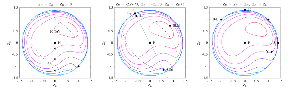
Figure 3: Bounds on $M_{Z^{\prime}}/g_{Z^{\prime}}$ in $\,{\rm TeV}$ at $99\%$ CL for different $Z^{\prime}$ models. Their effect dominantly depends on the charge of the Higgs and the leptons: we here assume the normalization $Z_{L}^{2}+Z_{E}^{2}+Z_{H}^{2}=2$ such that $Z_{H}=0$ at the boundary of the circles. The three plots, done assuming different sets of quark charges (zero, universal-like and SU(5)-unified) are almost identical, confirming the validity of an approximate analysis. The dashed line corresponds to a universal $Z^{\prime}$, and the dashed ellipse to a $Z^{\prime}$ compatible with SM Yukawa couplings. The dots show some well-known $Z^{\prime}$s.

In table 1 we report the $99\%$ CL bounds on $M_{Z^{\prime}}/g_{Z^{\prime}}$ for a set of $Z^{\prime}$s, theoretically motivated by extra dimensions, unification models, little Higgs models. We compare the bound obtained by performing an exact fit, that includes the effects of all the 18 relevant parameters, an approximate fit including the 9 parameters, and the purely oblique approximation. It is interesting to notice that the approximate bounds reproduce the exact one accurately in almost all the cases. There are few exceptions where the effect of quarks is relevant, and the oblique bound is overestimated. On the other hand, the 9-parameter approximation is always successful.

Fig. 3 shows iso-contours of bounds on $M_{Z^{\prime}}/g_{Z^{\prime}}$ (computed assuming a light Higgs) that approximately apply to all $Z^{\prime}$. Indeed the constraint dominantly depends only on the leptonic and Higgs $Z^{\prime}$ charges: $Z_{H},Z_{L},Z_{E}$. We here fixed their arbitrary overall normalization by assuming $Z_{H}^{2}+Z_{L}^{2}+Z_{E}^{2}=2$. Without loss of generality we can choose $Z_{H}\geq 0$, such that all the information lies on the surface of a half-sphere, and is plotted in fig. 3. The different panels show three different arbitrary choices for the quark $Z^{\prime}$ charges: vanishing (left panel), universal (middle panel), SU(5)-unified (right panel). Each panel shows the exact bound on $M_{Z^{\prime}}/g_{Z^{\prime}}$: one sees that there are very minor differences between the bounds in the three panels, confirming that leptonic data dominate the present global fit. The dots show the locations of the theoretically-motivated $Z^{\prime}$ listed in table 1. The dashed lines show special sub-classes of $Z^{\prime}$: universal $Z^{\prime}$ (oblique line) and $Z^{\prime}$s that do not forbid the SM Yukawa couplings (ellipse). For example, only two $Z^{\prime}$ have both these properties: a) the one denoted as $B^{\prime}$: a duplicate of the SM hypercharge; b) the one denoted as ‘SU6’ $Z^{\prime}$, that arises in little-Higgs models [6].

5 Proof for $W,Y\geq 0$

So far, the oblique parameters $W,Y$ have been computed in various models (in extra dimensions, Higgsless models, and litte Higgs at tree level [3, 6], and in supersymmetry [19] and Minimal Dark Matter [20] at one-loop level). In all of these cases it has been found that $W,Y\geq 0$. Next we discuss the general reason behind this result. The Källen–Lehmann representation implied by unitarity [21] tells us that propagators can be written as

$$\frac{1}{\Pi(p^{2})}=\int_{0}^{\infty}dm^{2}\frac{\rho(m^{2})}{p^{2}-m^{2}-i\varepsilon}\qquad\hbox{with}\qquad\rho(m^{2})\geq 0.$$ (5.1)

One can compute $\Pi^{\prime\prime}(0)$ and write in an appropriate form such that positivity is manifest:

$$\Pi^{\prime\prime}(0)=\frac{\int\!\int dm_{1}^{2}dm_{2}^{2}\,\rho(m_{1}^{2})\rho(m_{2}^{2})(m_{1}^{2}-m_{2}^{2})^{2}/m_{1}^{6}m_{2}^{6}}{[\int dm^{2}\,\rho(m^{2})/m^{2}]^{3}}\geq 0.$$

We could similarly prove that $\Pi^{\prime}(0)\geq 0$, and this indicates a potential caveat. The Källen–Lehmann representations applies to correlators of gauge invariant operators. In models where the SM gauge group is a subgroup of some larger non-abelian gauge group the relevant propagators are not gauge-invariant quantities: they can have matrix elements with unphysical negative-norm states, possibly giving $\Pi^{\prime\prime}(0)<0$. As well known, this is indeed what happens in the case of $\Pi^{\prime}(0)$, that contributes to the $\beta$-function of gauge couplings: non-abelian vectors negatively contribute to the $\beta$-function. Littlest-Higgs models with $T$-parity [22] might realize this caveat: the one-loop corrections to physical observables must be computed including the full gauge-invariant set of oblique, vertex and box diagrams.

6 Conclusions

We presented a simple and efficient general analysis of the constraints on heavy new physics from electroweak precision data measured below, at and above the $Z$-peak. We found that, out of a complete basis of 18 independent operators, precision data significantly constrain only about 10 combinations of new-physics parameters, see fig. 1. We have condensed the dominant precision data into 7 generalized oblique parameters $\hat{S},\hat{T},\hat{U},V,X,Y,W$ (that fully describe how new physics affects vectors and leptons), plus two parameters that describe the main corrections involving quarks: $\delta\varepsilon_{q}$, that describes corrections to the on-shell $q\bar{q}Z$ vertex, and $C_{q}$, that describes the size of $e\bar{e}q\bar{q}$ four fermion operators. A 10th parameter, the traditional $\delta\varepsilon_{b}$, is necessary if (as in most models) third generation quarks have unique properties.

We have shown that in most cases the simple oblique approximation (where only the seven oblique parameters are turned on) reasonably estimates the constraints on new physics, and that adding all 9 (or 10) parameters gives a bound that typically is within 10% of the exact bound. We have shown how to calculate these parameters from a generic set of higher dimensional operators, and emphasized that an added advantage of our parameters is that in many cases they can be directly computed via integrating out proper combinations of heavy new physics. We applied our methods giving approximate bounds on generic $Z^{\prime}$s (see fig. 3), and compared them with exact results in the specific cases of frequently-studied $Z^{\prime}$ (see table 1).

Finally, we have shown that first principles demand positivity constraints $W,Y\geq 0$ on these oblique parameters.

Appendix A The minimal parameters for a general Lagrangian

In this appendix we explicitly show how to transform a Lagrangian with generic ${\rm SU}(2)_{L}$-covariant dimension 6 operators to the parametrization advocated here. To start, we fix the notations for the dimension 6 operators. We define the Higgs and fermion currents as

$$J_{\mu H}=H^{\dagger}i\mathcal{D}_{\mu}H,\qquad J_{\mu H}^{a}=H^{\dagger}\tau^{a}i\mathcal{D}_{\mu}H,\qquad J_{\mu F}=\sum\bar{F}\gamma_{\mu}F,\qquad J_{\mu D}^{a}=\sum\bar{D}\gamma_{\mu}\tau^{a}D$$ (A.1)

where $\tau^{a}$ are the Pauli matrices (normalized such that $\mbox{Tr}\,(\tau^{a}\tau^{b})=2\delta^{ab}$), $F=\{E,L,Q,U,D\}$ and $D=\{L,Q\}$ and the currents are summed over the three flavors. In our notation the hypercharges are $Y_{E}=1$, $Y_{L}=-1/2$, $Y_{U}=-2/3$, $Y_{D}=1/3$, $Y_{Q}=1/6$, $Y_{H}=1/2$ and $\langle H\rangle=(0,v)$. As discussed in section 2, we split doublets $D=(u,d)$ in components and define

$$J_{\mu D}=J_{\mu}^{u_{L}}+J_{\mu}^{d_{L}}=\bar{u}_{L}\gamma_{\mu}u_{L}+\bar{d}_{L}\gamma_{\mu}d_{L},\qquad J^{-}_{\mu D}=\bar{u}_{L}\gamma_{\mu}d_{L},\qquad J^{+}_{\mu D}=\bar{d}_{L}\gamma_{\mu}u_{L}$$

To shorten the notation, we define $s=\sin\theta_{W}$, $c=\cos\theta_{W}$ and $t=\tan\theta_{W}$.

We start from a complete list of dimension 6 operators that are relevant for the precision measurements at LEP: following the notation of [1, 2], the operators are

• 7 operators involving one fermion current (vertex operators):

  $$\mathcal{O}_{HF}=J_{\mu H}J_{\mu F}+\hbox{h.c.}=-2\frac{M_{W}^{2}}{g^{2}}(gW^{3}_{\mu}-g^{\prime}B_{\mu})J_{f}^{\mu}\,+\cdots\\$$ (A.2)

  where $F=\{L,E,Q,U,D\}$ and

  $$\mathcal{O}^{\prime}_{HD}=J_{\mu H}^{a}J^{a}_{\mu D}+\hbox{h.c.}=2\frac{M_{W}^{2}}{g^{2}}(gW^{3}_{\mu}-g^{\prime}B_{\mu})(J_{\mu}^{u_{L}}-J_{\mu}^{d_{L}})+4\frac{M_{W}^{2}}{g^{2}}\frac{g}{\sqrt{2}}\left(W^{+}_{\mu}J^{-}_{D\mu}+\hbox{h.c.}\right)+\cdots$$ (A.3)

  where $D=\{L,Q\}$.

• 11 operators involving two fermion currents (4-fermion operators):

  $$\mathcal{O}_{FF^{\prime}} = \frac{J_{\mu F}J_{\mu F^{\prime}}}{1+\delta_{FF^{\prime}}}$$ (A.4)

  $$\mathcal{O}^{\prime}_{DD^{\prime}} = \frac{J^{a}_{\mu D}J^{a}_{\mu D^{\prime}}}{1+\delta_{DD^{\prime}}}=\frac{(J^{u_{L}}-J^{d_{L}})\cdot(J^{u^{\prime}_{L}}-J^{d^{\prime}_{L}})+2(J^{+}_{D}\cdot J^{-}_{D^{\prime}}+J^{-}_{D}\cdot J^{+}_{D^{\prime}})}{1+\delta_{DD^{\prime}}}.$$ (A.5)

  Precision data at and below the $Z$-peak are affected only by $\mathcal{O}^{\prime}_{LL}$ [1]. To study also LEP2 data above the $Z$-peak, [2] added 10 more 4-fermion operators. The full list of the 11 4-fermion operators involving leptons is then given by:

  $$\mathcal{O}_{EE},\mathcal{O}_{LL},\mathcal{O}_{EL},\mathcal{O}_{EU},\mathcal{O}_{ED},\mathcal{O}_{EQ},\mathcal{O}_{LU},\mathcal{O}_{LD},\mathcal{O}_{LQ},\mathcal{O}^{\prime}_{LL},\mathcal{O}^{\prime}_{LQ}$$

In total this makes 18 operators. We here also consider 4 more oblique operators (i.e.  operators that do not involve fermions):

$$\halign to=0.0pt{\@eqnsel\hskip\@centering$\displaystyle{#}$&\global\@eqcnt\@ne\hskip 2\arraycolsep\hfil${#}$\hfil& \global\@eqcnt\tw@\hskip 2\arraycolsep$\displaystyle{#}$\hfil&\llap{#}\cr 0.0pt plus 1000.0pt$\displaystyle{\mathcal{O}_{WB} &10.0pt\hfil${=&10.0pt$\displaystyle{\left( H^{\dagger}\tau^{a} H \right)\, W^{a}_{\mu\nu} B^{\mu\nu} = -2 \frac{M_{W}^{2}}{g^{2}}\, W^{3}_{\mu\nu} B^{\mu\nu} +\cdots\,;\\ \mathcal{O}_{HH} &\hbox to0.0pt{\hss=&|J_{\mu H}|^{2}=\left(\frac{M_{W}^{2}}{g^{2}}\right)^{2}(gW^{3}_{\mu}-g^{\prime}B_{\mu})^{2}+\cdots\,;\\\mathcal{O}_{WW}&=&\frac{(\mathcal{D}_{\rho}W^{a}_{\mu\nu})^{2}}{2}\\\mathcal{O}_{BB}&=&\frac{(\mathcal{D}_{\rho}B_{\mu\nu})^{2}}{2}&(A.6)\cr}}}}}$$

Using the equations of motion for the two neutral gauge bosons (see [5] for a recent discussion), these oblique operators can be reduced to combinations of the previous 18, up to poorly constrained operators, e.g. operators that affect couplings among vectors:

$$iB_{\mu\nu}\mathcal{D}^{\mu}H^{\dagger}\mathcal{D}^{\nu}H,\qquad iW^{a}_{\mu\nu}\mathcal{D}^{\mu}H^{\dagger}\tau^{a}\mathcal{D}^{\nu}H.$$ (A.7)

This operator basis can be converted into the basis discussed in the main text by using the equations of motion for the gauge bosons $W^{\pm},W^{3},B$ to eliminate all the charged lepton currents from $\mathscr{L}_{\rm BSM}$. At leading order in the operator coefficients, we only need the equations of motion that follow from $\mathscr{L}_{\rm SM}$:

$$\halign to=0.0pt{\@eqnsel\hskip\@centering$\displaystyle{#}$&\global\@eqcnt\@ne\hskip 2\arraycolsep\hfil${#}$\hfil& \global\@eqcnt\tw@\hskip 2\arraycolsep$\displaystyle{#}$\hfil&\llap{#}\cr 0.0pt plus 1000.0pt$\displaystyle{\partial^{\nu}B_{\nu\mu} + \frac{M_{W}^{2}}{g^{2}} g' (g' B_{\mu}- g W^{3}_{\mu}) + g' \sum_{F} Y_{F} J^{f}_{\mu} &10.0pt\hfil${=&10.0pt$\displaystyle{0 +\ldots\\ \partial^{\nu}W^{3}_{\nu\mu} + \frac{M_{W}^{2}}{g^{2}} g (g W^{3}_{\mu}- g' B_{\mu}) + g \sum_{f} T_{3} J^{f}_{\mu}&\hbox to0.0pt{\hss=&0+\ldots\\\partial^{\nu}W^{\pm}_{\nu\mu}+M_{W}^{2}W^{+}_{\mu}+\frac{g}{\sqrt{2}}\sum_{F}J^{\pm}_{\mu F}&=&0+\ldots&(A.8)\cr}}}}}$$

where we neglected on the r.h.s. operators that are poorly measured. We now solve the equations of motion in terms of

$$J^{e_{R}}_{\mu}\equiv J_{\mu E}=\bar{e}_{R}\gamma_{\mu}e_{R},\qquad J^{e_{L}}_{\mu}\equiv\bar{e}_{L}\gamma_{\mu}e_{L},\qquad J^{+}_{L\mu}\equiv\bar{e}_{L}\gamma_{\mu}\nu_{L}$$ (A.9)

and plug the result into the Lagrangian generated by the new physics. In this way we replace $\mathscr{L}_{\rm BSM}$ with an equivalent version that does not contain corrections to $Ze^{+}e^{-}$ and $W^{+}e^{-}\nu$ vertices nor 4-fermion operators involving charged leptons. The effects of new physics have been completely recast on the propagators of the gauge bosons and in the couplings of the gauge bosons to quarks and neutrinos, and we obtain a Lagrangian in the form of eq. (2.2). Thus, we can read off the parameters of section 2 in terms of the coefficients of the operators we listed above.

A.1 Oblique corrections and neutrinos

For the oblique parameters we find:

$$\halign to=0.0pt{\@eqnsel\hskip\@centering$\displaystyle{#}$&\global\@eqcnt\@ne\hskip 2\arraycolsep\hfil${#}$\hfil& \global\@eqcnt\tw@\hskip 2\arraycolsep$\displaystyle{#}$\hfil&\llap{#}\cr 0.0pt plus 1000.0pt$\displaystyle{\hat{S} &10.0pt\hfil${=&10.0pt$\displaystyle{\frac{M_{W}^{2}}{g g'}\bigg{[}4c_{WB} + 4 t\, (c'_{HL}- c'_{LL}) + \frac{2}{t}\, (c_{HE}-c_{EE}- c_{EL} ) + \\ &\hbox to0.0pt{\hss&+2t\,(c_{HE}+2c_{HL}-c_{EE}-2c_{LL}-3c_{EL})\bigg{]}\,,\\\hat{T}&=&\frac{M_{W}^{2}}{g^{2}}\bigg{[}-2c_{HH}+8(c_{HL}+c_{HE})-4(c_{LL}+c_{EE}+2c_{EL})\bigg{]}\,,\\\hat{U}&=&\frac{M_{W}^{2}}{g^{2}}\bigg{[}4(c_{HE}+2c_{HL})-4(c_{EE}+2c_{LL}+3c_{EL})\bigg{]}\,,\\V&=&-\frac{M_{W}^{2}}{g^{2}}\bigg{[}c_{EE}+4c_{LL}+4c_{EL}\bigg{]}\,,\\X&=&\frac{M_{W}^{2}}{gg^{\prime}}\bigg{[}c_{EE}+2c_{EL}\bigg{]}\,,\\Y&=&\frac{M_{W}^{2}}{g^{\prime 2}}\bigg{[}2c_{BB}{g^{\prime}}^{2}-c_{EE}\bigg{]}\,,\\W&=&\frac{M_{W}^{2}}{g^{2}}\bigg{[}2c_{WW}g^{2}-4c^{\prime}_{LL}-(c_{EE}+4c_{LL}+4c_{EL})\bigg{]}.&(A.10)\cr}}}}}$$

Next, we give the expressions for the non-oblique terms defined in eq. (2.6). The correction to the on-shell neutrino/$Z$ couplings is

$$\delta g_{L\nu} = -\frac{2M_{W}^{2}}{g^{2}}\Big{[}c_{HE}+2c_{HL}\Big{]}\,=V-\frac{1}{2}\hat{U}-tX\,.$$ (A.11)

We see that it can be re-expressed in terms of the oblique parameters. This is true also for the corrections to the off-shell couplings $C^{\gamma}_{L\nu}$ and $C^{Z}_{L\nu}$: we do not give their explicit expressions because experiments negligibly constrain them. This shows that the 7 oblique parameters fully describe charged leptons and neutrinos.

A.2 Vertex corrections

As discussed in the text, in the quark sector our approximation includes only two more important combinations of effects. They are:

$$\delta\varepsilon_{q} = \frac{2M_{W}^{2}}{g^{2}}\Big{[}2(c^{\prime}_{HQ}-c^{\prime}_{HL})-(c_{HE}+2c_{HL})\Big{]}\,=$$

$$= \frac{4M_{W}^{2}}{g^{2}}(c^{\prime}_{HQ}-c^{\prime}_{HL})+V-\frac{1}{2}\hat{U}-tX\,,$$

$$\delta C_{q} = \frac{2M_{W}^{2}}{g^{2}+{g^{\prime}}^{2}}\Big{[}2(c^{\prime}_{LQ}-c^{\prime}_{LL})-(c_{EE}+3c_{LE}+2c_{LL})\Big{]}\,=$$

$$= \frac{4M_{W}^{2}}{g^{2}+{g^{\prime}}^{2}}(c^{\prime}_{LQ}-c^{\prime}_{LL})+c^{2}V-csX\,.$$

Besides oblique terms, they only depend on the operators involving SU(2)_L currents. The oblique approximation, therefore, fails only in the SU(2) sector.

For completeness, we also list the other parameters in the quark sector that we neglect: the 6 parameters involving left-handed quarks are

$$\delta g_{Lq} = -2\frac{M_{W}^{2}}{g^{2}}\Big{[}(c_{HQ}-Y_{Q}c_{HE})\pm(c^{\prime}_{HL}-c^{\prime}_{HQ})\pm\frac{1}{2}\,(c_{HE}+2c_{HL})\Big{]}\,,$$ (A.14)

$$C^{\gamma}_{Lq} = \frac{M_{W}^{2}}{e^{2}}\Big{[}(c_{EQ}-Y_{Q}c_{EE})(c^{2}-s^{2})-2(c_{LQ}-Y_{Q}c_{LE})s^{2}\pm 2(c^{\prime}_{LQ}-c^{\prime}_{LL})s^{2}+$$ (A.15)

$$\pm\frac{c^{2}}{2}(c_{EE}+2c_{EL})\mp\frac{s^{2}}{2}(c_{EE}+4c_{LL}+4c_{EL})\Big{]}\,,$$

$$C^{Z}_{Lq} = -\frac{2M_{W}^{2}}{g^{2}+{g^{\prime}}^{2}}\Big{[}(c_{EQ}+c_{LQ})-Y_{Q}(c_{EE}+c_{LE})\pm(c^{\prime}_{LL}-c^{\prime}_{LQ})+$$ (A.16)

$$\pm\frac{1}{2}(c_{EE}+3c_{LE}+2c_{LL})\Big{]}\,,$$

where $q$ stands for $u$ and $d$ and the signs refer to the up/down component of the doublet. They depend on 5 coefficients $c_{HQ}$, $c^{\prime}_{HQ}$, $c_{EQ}$, $c_{LQ}$, $c^{\prime}_{LQ}$: only the differences $C^{Z}_{Lu}-C^{Z}_{Ld}$ and $C^{\gamma}_{Lu}-C^{\gamma}_{Ld}$ depend on $c^{\prime}_{LQ}$, and are related by

$$(C^{\gamma}_{uL}-C^{\gamma}_{dL})=c^{2}(C^{Z}_{uL}-C^{Z}_{dL})-\frac{1}{t}X\,.$$ (A.17)

In practice, we neglect $C^{Z}_{Lu}+C^{Z}_{Ld}$ and $C^{\gamma}_{Lu}+C^{\gamma}_{Ld}$, and $C^{\gamma}_{Lu}-C^{\gamma}_{Ld}$ is determined in terms of $\delta C_{q}$ and oblique parameters.

The corrections to the right-handed quark couplings are described by the following 6 parameters:

$$\delta g_{Rq} = -2\frac{M_{W}^{2}}{g^{2}}\Big{[}c_{Hq}-Y_{q}c_{HE}\Big{]}\,,$$ (A.18)

$$C^{\gamma}_{Rq} = \frac{M_{W}^{2}}{e^{2}}\Big{[}(c_{Eq}-Y_{q}c_{EE})(c^{2}-s^{2})-2(c_{Lq}-Y_{q}c_{EL})s^{2}\Big{]}\,,$$ (A.19)

$$C^{Z}_{Rq} = -\frac{2M_{W}^{2}}{g^{2}+{g^{\prime}}^{2}}\Big{[}c_{Eq}+c_{Lq}-Y_{q}(c_{EE}+c_{EL})\Big{]}\,,$$ (A.20)

where $q$ stands for $U$ and $D$. They depend on the 6 coefficients $c_{HU}$, $c_{HD}$, $c_{EU}$, $c_{ED}$, $c_{LU}$, $c_{LD}$, and are independent. Their effect on precisio measurements is negligible.

Corrections to the quark/$W$ couplings are determined in terms of our parameters: we do not give explicit expressions as experiments negligibly constrain these couplings.

For the bottom, $\delta\varepsilon_{b}$ can be read off from eq. (A.14):

$$\delta\varepsilon_{b}=\frac{M_{W}^{2}}{g^{2}}\Big{[}(c^{\prime}_{HQ_{3}}-c^{\prime}_{HL})+c_{HQ_{3}}-c_{HL}-\frac{2}{3}c_{HE}\Big{]}\,.$$ (A.21)

In the flavour universal limit, it can be written in terms of the light quark parameters in the following way:

$$\delta\varepsilon_{b} = \delta\varepsilon_{q}-(\delta g_{uL}+\delta g_{dL})\,.$$ (A.22)

A.3 The universal limit

One can verify that in the limit of heavy universal new physics, our expressions reduce to the $\hat{S},\hat{T},W,Y$ parameters only, with all other parameters vanishing. Indeed in the ‘universal’ case only the following combinations of currents can appear in $\mathscr{L}_{\rm BSM}$:

$$J_{Y}^{\mu}=\sum_{f}Y_{F}J_{F}^{\mu},\;\;\;\;\;J^{a}=\sum_{D}J_{D}^{\mu,a}.$$ (A.23)

This restricts the coefficients of the operators to be of the form

$$c_{HF}=Y_{F}\,c_{v}\,,\quad c^{\prime}_{HF}=c^{\prime}_{v}\,,\quad c_{FF^{\prime}}=Y_{F}Y_{F^{\prime}}\,c_{4f}\,,\quad c^{\prime}_{FF^{\prime}}=c^{\prime}_{4f}\,,$$ (A.24)

such that the non-vanishing $\hat{S},\hat{T},W,Y$ parameters are

$$\halign to=0.0pt{\@eqnsel\hskip\@centering$\displaystyle{#}$&\global\@eqcnt\@ne\hskip 2\arraycolsep\hfil${#}$\hfil& \global\@eqcnt\tw@\hskip 2\arraycolsep$\displaystyle{#}$\hfil&\llap{#}\cr 0.0pt plus 1000.0pt$\displaystyle{\hat{S} &10.0pt\hfil${=&10.0pt$\displaystyle{\frac{M_{W}^{2}}{g g'}\bigg{[}4 c_{WB} + 4 t\, (c'_{v} - c'_{4f}) + \frac{2}{t}\, c_{v} - \frac{1}{t}\, c_{4f} \bigg{]} \,,\\ \hat{T} &\hbox to0.0pt{\hss=&\frac{M_{W}^{2}}{g^{2}}\bigg{[}-2c_{HH}+4c_{v}+c_{4f}\bigg{]}\,,\\Y&=&\frac{M_{W}^{2}}{g^{\prime 2}}\bigg{[}2c_{BB}{g^{\prime}}^{2}-c_{4f}\bigg{]}\,,\\W&=&\frac{M_{W}^{2}}{g^{2}}\bigg{[}2c_{WW}g^{2}-c^{\prime}_{4f}\bigg{]}.&(A.25)\cr}}}}}$$

These expressions explicitly show how the 4 oblique operators in eq. (A) are equivalent to appropriate universal combinations of non-oblique operators.

References

- [1] R. Barbieri and A. Strumia, Phys. Lett. B 462 (1999) 144 [hep-ph/9905281].
- [2] Z. Han and W. Skiba, Phys. Rev. D 71 (2005) 075009 [hep-ph/0412166].
- [3] R. Barbieri, A. Pomarol, R. Rattazzi and A. Strumia, Nucl. Phys. B 703 (2004) 127 [hep-ph/0405040].
- [4] M. E. Peskin and T. Takeuchi, Phys. Rev. Lett. 65, 964 (1990).
- [5] C. Grojean, W. Skiba and J. Terning, hep-ph/0602154.
- [6] G. Marandella, C. Schappacher and A. Strumia, Phys. Rev. D 72 (2005) 035014 [hep-ph/0502096].
- [7] R. Barbieri, A. Pomarol and R. Rattazzi, Phys. Lett. B 591 (2004) 141 [hep-ph/0310285].
- [8] G. Altarelli, R. Barbieri and F. Caravaglios, Nucl. Phys. B 405 (1993) 3.
- [9] W. Buchmüller, D. Wyler, Nucl. Phys. B268 (1986) 621.
- [10] T. E. W. Group, hep-ex/0603039.
- [11] NuTeV collaboration, Phys. Rev. Lett. 88 (2002) 091802 [Erratum-ibid. 90 (2003) 239902] [hep-ex/0110059].
- [12] for a review, see M. Schmaltz and D. Tucker-Smith, hep-ph/0502182.
- [13] C. Csaki, C. Grojean, L. Pilo and J. Terning, Phys. Rev. Lett. 92, 101802 (2004) [hep-ph/0308038]; G. Cacciapaglia, C. Csaki, C. Grojean and J. Terning, Phys. Rev. D 71, 035015 (2005) [hep-ph/0409126].
- [14] M. Schmaltz, JHEP 0408, 056 (2004) [hep-ph/0407143].
- [15] G. Altarelli and R. Barbieri, Phys. Lett. B 253, 161 (1991).
- [16] K. Agashe, R. Contino and A. Pomarol, Nucl. Phys. B 719, 165 (2005) [hep-ph/0412089]; K. Agashe and R. Contino, hep-ph/0510164.
- [17] G. Cacciapaglia, C. Csaki and S. C. Park, JHEP 0603, 099 (2006) [hep-ph/0510366]; G. Panico, M. Serone and A. Wulzer, Nucl. Phys. B 739, 186 (2006) [hep-ph/0510373].
- [18] C. Csaki, G. Marandella, Y. Shirman and A. Strumia, Phys. Rev. D 73, 035006 (2006) [hep-ph/0510294].
- [19] G. Marandella, C. Schappacher and A. Strumia, Nucl. Phys. B 715 (2005) 173 [hep-ph/0502095].
- [20] M. Cirelli, N. Fornengo and A. Strumia, hep-ph/0512090.
- [21] See e.g. the book by M.E. Peskin, D.V. Schroeder, ‘An introduction to Quantum Field Theory’.
- [22] I. Low, JHEP 0410, 067 (2004) [hep-ph/0409025]; J. Hubisz, P. Meade, A. Noble and M. Perelstein, JHEP 0601, 135 (2006) [hep-ph/0506042].