Nuclear shadowing

Abstract

The phenomenon of shadowing of nuclear structure functions at small values of Bjorken-$x$ is analyzed. First, multiple scattering is discussed as the underlying physical mechanism. In this context three different but related approaches are presented: Glauber-like rescatterings, Gribov inelastic shadowing and ideas based on high-density Quantum Chromodynamics. Next, different parametrizations of nuclear partonic distributions based on fit analysis to existing data combined with Dokshitzer-Gribov-Lipatov-Altarelli-Parisi evolution, are reviewed. Finally, a comparison of the different approaches is shown, and a few phenomenological consequences of nuclear shadowing in high-energy nuclear collisions are presented.

1 Introduction

The fact that nuclear structure functions in nuclei are different from the superposition of those of their constituents nucleons is a well known phenomenon since the early seventies, see references in the reviews [1, 2]. For example, for $F_{2}$ the nuclear ratio is defined as the nuclear structure function per nucleon divided by the nucleon structure function,

$$R_{F_{2}}^{A}(x,Q^{2})={F_{2}^{A}(x,Q^{2})\over A\,F_{2}^{\rm nucleon}(x,Q^{2})}\,.$$ (1)

Here, $A$ is the nuclear mass number (number of nucleons in the nucleus). The variables $x$ and $Q^{2}$ are defined as usually in leptoproduction or deep inelastic scattering (DIS) experiments: in the scattering of a lepton with four-momentum $k$ on a nucleus with four-momentum $Ap$ mediated by photon exchange (the dominant process at $Q^{2}\ll m_{{\rm Z}^{0}}^{2},m_{\rm W}^{2}$ where most nuclear data exist),

$$l(k)+A(Ap)\longrightarrow l(k^{\prime})+X(Ap^{\prime}),$$

$$q=k-k^{\prime},\ \ W^{2}=(q+p)^{2},\ \ x={-q^{2}\over 2p\cdot q}={-q^{2}\over W^{2}-q^{2}-m_{\rm nucleon}^{2}},$$ (2)

see Fig. 1. The variable $x$ has the meaning of the momentum fraction of the nucleon in the nucleus carried by the parton with which the photon has interacted. $Q^{2}=-q^{2}>0$ represents the squared inverse resolution of the photon as a probe of the nuclear content. And $W^{2}$ is the center-of-mass-system energy of the virtual photon-nucleon collision (lepton masses have been neglected and $m_{\rm nucleon}$ is the nucleon mass), see e.g. [3] for full explanations. The nucleon structure function is usually defined through measurements on deuterium, $F_{2}^{\rm nucleon}=F_{2}^{\rm deuterium}/2$, assuming nuclear effects in deuterium to be negligible.

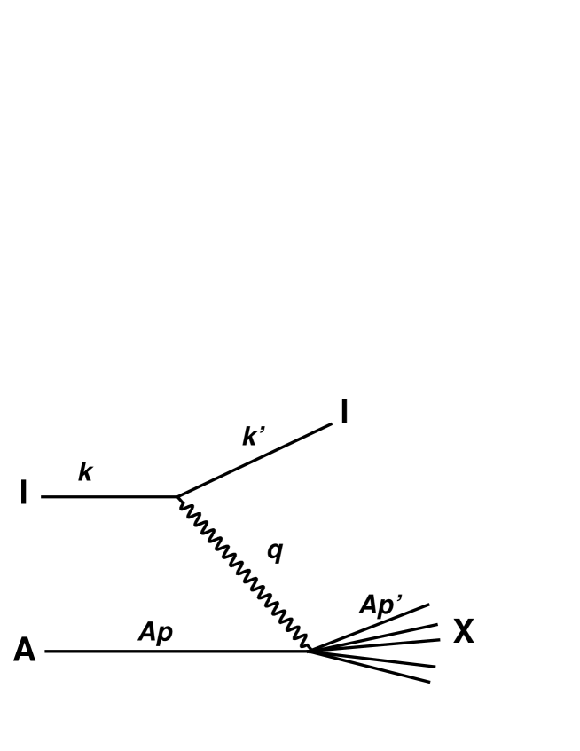
Figure 1: Diagram of leptoproduction on a nucleus through virtual photon exchange.

The behaviour of $R_{F_{2}}^{A}(x,Q^{2})$ as a function of $x$ for a given fixed $Q^{2}$ is shown schematically in Fig. 2. It can be divided into four regions:

• $R_{F_{2}}^{A}>1$ for $x\gtrsim 0.8$: the Fermi motion region.

• $R_{F_{2}}^{A}<1$ for $0.25\div 0.3\lesssim x\lesssim 0.8$: the EMC region (EMC stands for European Muon Collaboration).

• $R_{F_{2}}^{A}>1$ for $0.1\lesssim x\lesssim 0.25\div 0.3$: the antishadowing region.

• $R_{F_{2}}^{A}<1$ for $x\lesssim 0.1$: the shadowing region.

Figure 2: Schematic behaviour of $R_{F_{2}}^{A}(x,Q^{2})$ as a function of $x$ for a given fixed $Q^{2}$.

This review will be focused in the small $x$ region i.e. that of shadowing, see [1, 2] for discussions on the other regions. The most recent experimental data [4, 5, 6, 7, 8, 9] (see [1, 2, 10, 11, 12] for previous experimental results), confined to a limited region of not very low $x$ and small or moderate $Q^{2}$ (and with a strong kinematical correlation between small $x$ and small $Q^{2}$, see Fig. 3), indicate that: i) shadowing increases with decreasing $x$, though at the smallest available values of $x$ the behaviour is compatible with either a saturation or a mild decrease [8]; ii) shadowing increases with the mass number of the nucleus [6]; and iii) shadowing decreases with increasing $Q^{2}$ [7]. On the other hand, the existing experimental data do not allow a determination of the dependence of shadowing on the centrality of the collision.

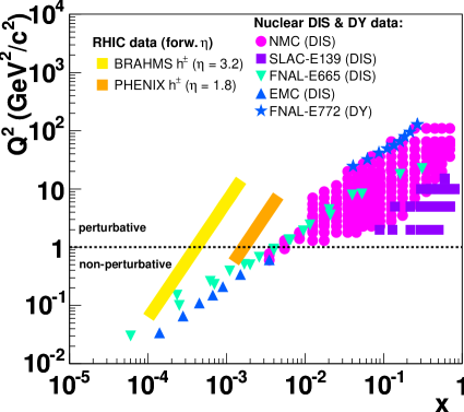
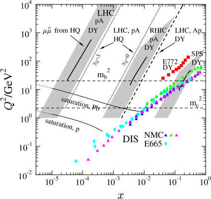
Figure 3: Plot on the left: Kinematical range in the $x$-$Q^{2}$ plane probed in nuclear DIS [4, 5, 6, 7, 8, 9, 10, 11, 12] and Drell-Yan [13] processes, and in d-Au at forward rapidities [14, 15] at RHIC. [Figure taken from [16].] Plot on the right: The average values of $x$ and $Q^{2}$ of the DIS data from the New Muon Collaboration [4, 5, 6, 7] (triangles) and E665 [8, 9] (diamonds) in $l$-$A$, and of $x_{2}$ and $M^{2}$ of the Drell-Yan dilepton data [13] (squares) in p-$A$. The heavy quark mass scales are shown by the horizontal dashed lines. Those lines labeled saturation indicate the estimated saturation scale in proton and Pb. The different bands and lines show the values of $x$ and $Q^{2}$ which are or will be probed in Drell-Yan or heavy flavour production at SPS, RHIC and LHC, for rapidities different from central ones when indicated. [Figure taken from [17].] See also the text in Subsection 2.3 and in Section 5.

In the region of small $x$, partonic distributions are dominated by sea quarks and gluons. Thus isospin effects, partially corrected in practice by the use of deuterium as reference and of isoscalar nuclei, are negligible and will not be discussed in the following. In most approaches, the origin of the depletion of the nuclear ratios in this region is related with the hadronic behaviour of the virtual photon [18]. This resolved hadronic component of the photon wave function at high collision energies - equivalent to small values of $x$, see (2) - and at relatively low values of $Q^{2}$, will interact several times with the different nucleons in the nucleus i.e. will experience multiple scattering. As I will discuss in the next Section, this results in a reduction of the corresponding cross sections - shadowing, related to the structure functions through

$$F^{A}_{2}(x,Q^{2})={Q^{2}(1-x)\over 4\pi^{2}\alpha_{\rm EM}}\,\sigma_{\gamma^{*}-A}\,,$$ (3)

with $\alpha_{\rm EM}$ the fine structure constant. Thus, the phenomenon of multiple scattering is sometimes referred to as shadowing corrections.

The importance of the phenomenon of nuclear shadowing is twofold: First, on the theoretical side it offers an experimentally accessible testing ground for our understanding of Quantum Chromodynamics (QCD) in the high-energy regime [19]. Multiple scattering is unavoidable in a quantum field theory as a consequence of such a basic requirement of the theory as unitarity. The nuclear size gives the possibility to control the amount of multiple scattering at given values of momentum fraction $x$ and scale $Q$. Besides, by varying the scale and the energy of the collision the interplay between the soft non-perturbative and the hard perturbative regimes can be addressed. Second, experimental studies on high-energy nuclear collisions like those at the Relativistic Heavy Ion Collider (RHIC) [20, 21, 22, 23] at the Brookhaven National Laboratory (BNL) are presently carried out. New possibilities like the Large Hadron Collider (LHC) [17] at CERN or the Electron-Ion Collider (EIC) [24] under consideration, will become available in the future. They test the behaviour of parton densities inside nuclei at larger energies/smaller $x$ than those presently available in fixed target studies like those at the Super Proton Synchrotron (SPS) at CERN. These new experimental data offer the possibility to further constrain our knowledge on the behaviour of nuclear cross sections and structure functions, both for observables characterized by a large scale for which standard perturbation theory can be applied, and for those with intermediate and small scales where new methods have been developed.

The plan of the review is the following: In Section 2 models based on multiple scattering will be reviewed. In Section 3 those models which do not try to address the origin of nuclear shadowing but rather to study its evolution through the Dokshitzer-Gribov-Lipatov-Altarelli-Parisi (DGLAP) equations [25, 26, 27], will be discussed. A comparison of the different models will be shown in Section 4. Next, some consequences on high-energy nuclear collisions will be presented in Section 5. Finally, in Section 6 some conclusions will be drawn. I have mainly focused on the most recent approaches roughly starting from the early nineties, please have a look at [1] for an extensive list of references on earlier theoretical and experimental work.

2 Models based on multiple scattering

As commented in the Introduction, the usual explanation for the origin of shadowing is multiple scattering [28, 29, 30, 31, 32, 33, 34, 35, 36, 37, 38, 39, 40, 41, 42, 43, 44, 45, 46, 47, 48, 49, 50, 51, 52, 53, 54, 55]. While the basis of the explanation is common, phenomenological details of its application vary from model to model. For example, the hadronic component of the virtual photon may be given a partonic structure like in the dipole model [36], see the next Subsection, or modeled [28, 29, 31, 32, 33] as a superposition of hadronic states with the photon quantum numbers - vector meson dominance, or some combination of both approaches e.g. [34]. Besides, what is seen as multiple scattering in the rest frame of the nucleus corresponds to recombination in the infinite momentum frame [49, 50]. Just to mention a few differences between the results of the models, the behaviour of models [36, 37, 38] is dominated by hadronic configurations of large size, so the results turns out to be basically $Q^{2}$-independent. On the other hand, models which consider an expansion in power-suppressed corrections in $1/Q$, either a fixed number of terms [50, 51, 52] or some re-summation [54], show a clear $Q^{2}$ dependence. Some models rely on an eikonal approximation [39, 41, 54], see below, and are unable to reproduce the return of $F_{2}$ nuclear ratios to 1 at $x\sim 0.1$, while others [42, 43, 44, 45, 46, 47, 48] include effects of finite coherence length, see below, and are able to reproduce such a behaviour.

In this Section I will start by working out a little exercise which shows how multiple scattering leads to shadowing. This exercise should also clarify the origin of coherence effects. Then, in the Subsections models based on Glauber-like rescatterings, on Gribov inelastic shadowing, and finally the ideas based on high-energy QCD [19], will be reviewed.

For the exercise I consider the contribution coming from one and two scatterings, to the high-energy cross section of a massless scalar particle on a nucleus with mass number $A$. The scattering centers plus the interaction vertex are represented by the projectile-nucleon forward scattering amplitude times the nuclear density (see Fig. 4). This example follows the spirit of the Glauber-Gribov theory [57, 58, 59]; technical details can be found in Section 3.1 and Appendix A in [60] for the case of scalar QCD at high energy.

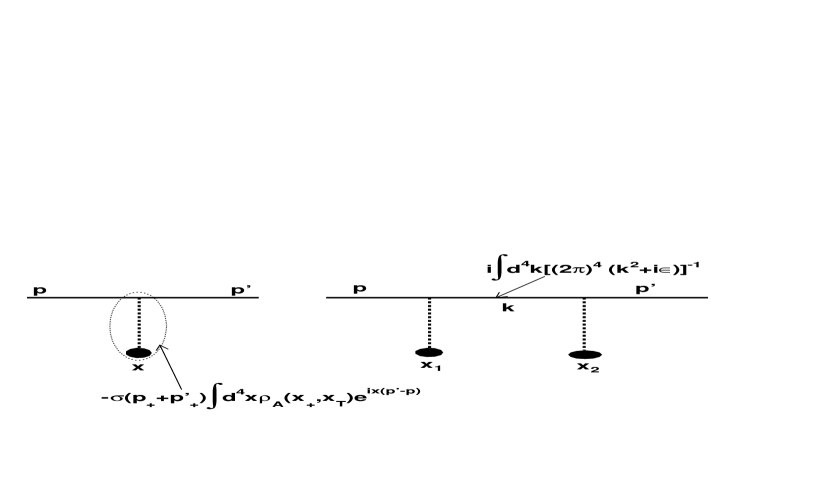
Figure 4: One- (left) and two- (right) scattering diagrams, with the corresponding Feynman rules written on them.

I will use light-cone coordinates $a_{\pm}=a_{0}\pm a_{z}$, $a=(a_{0},a_{T},a_{z})=(a_{+},a_{-},a_{T})$ with $a_{T}=(a_{x},a_{y})$ the two-dimensional transverse vector, assume dominance of the $+$-components for the projectile, and define $q=p^{\prime}-p$. I will employ the optical theorem for purely imaginary amplitudes, $i{t}(q=0)=it_{\rm forw}=-\sigma$ for projectile-nucleon and $i{\cal T}_{n}(q=0)=-\sigma_{A}^{n}$ for the $n$-scattering contribution for projectile-nucleus collisions. Then the amplitude with one scattering (Fig. 4 left) reads:

$$c(p_{+},p^{\prime}_{+})i{\cal T}_{1}(q) = i{t}_{\rm forw}\ A(p_{+}+p^{\prime}_{+})\int d^{4}x\,\rho_{A}(x_{+},x_{T})e^{ix\cdot(p^{\prime}-p)}$$ (4)

$$= i{t}_{\rm forw}\ c(p_{+},p^{\prime}_{+})A\int d^{2}x_{T}\,T_{A}(x_{T})e^{-ix_{T}\cdot(p_{T}^{\prime}-p_{T})}.$$

$\rho_{A}(x_{+},x_{T})$ is the nuclear density normalized to 1,

$$T_{A}(x_{T})=\int_{-\infty}^{+\infty}dx_{+}\,\rho_{A}(x_{+},x_{T})$$ (5)

the nuclear profile, $|x_{T}|=b$ the impact parameter and $c(p_{+},p^{\prime}_{+})=(2\pi)2p_{+}\delta(p^{\prime}_{+}-p_{+})$ a normalization factor. For the forward scattering case $q=0$, (4) gives

$$\sigma_{A}^{1}=A\,\sigma$$ (6)

as expected. The two-scattering contribution (Fig. 4 right) reads

$$c(p_{+},p^{\prime}_{+})i{\cal T}_{2}(q)=iA(A-1)(i{t}_{\rm forw})^{2}\int{d^{4}k\over(2\pi)^{4}}d^{4}x_{1}d^{4}x_{2}\,e^{ix_{1}\cdot(k-p)}$$

$$\times e^{ix_{2}\cdot(p^{\prime}-k)}{(p_{+}+k_{+})(k_{+}+p^{\prime}_{+})\over k^{2}+i\epsilon}\rho_{A}(x_{1+},x_{1T})\rho_{A}(x_{2+},x_{2T})$$

$$=c(p_{+},p^{\prime}_{+})A(A-1)(i{t}_{\rm forw})^{2}$$ (7)

$$\times\int{d^{2}k_{T}\over(2\pi)^{2}}dx_{1+}dx_{2+}d^{2}x_{1T}d^{2}x_{2T}\,e^{-ik_{T}^{2}(x_{2+}-x_{1+})/(2p_{+})}$$

$$\times e^{-i[x_{1T}\cdot(k_{T}-p_{T})+x_{2T}\cdot(p^{\prime}_{T}-k_{T})]}\rho_{A}(x_{1+},x_{1T})\rho_{A}(x_{2+},x_{2T})\theta(x_{2+}-x_{1+}),$$

with $\theta(x)$ the step function. The second equality follows from doing the $dk_{-}$ integral closing the integration contour with an infinite semicircle in the lower half-plane and simplifying the remaining $\delta$-functions.

Coherence effects are contained in the factor $\exp{[-ik_{T}^{2}(x_{2+}-x_{1+})/(2p_{+})]}$ which can be written as $\exp{[-i(x_{2+}-x_{1+})/l_{c}]}$, with $l_{c}=2p_{+}/k_{T}^{2}$ the coherence length. In the low energy limit $p_{+}\to 0$ this factor leads to $i{\cal T}_{2}(q)\to 0$ (the same happens for contributions with more than two scatterings). Then all rescattering corrections vanish, so the total cross section results equal to the superposition of single scatterings (6) - this limit is thus called the incoherent limit. This would imply a nuclear ratio equal to 1, so shadowing vanishes for low energies i.e. large values of $x$. On the other hand, in the large energy, totally coherent limit $p_{+}\to\infty$, $\exp{[-i(x_{2+}-x_{1+})/l_{c}]}\to 1$ and (7) gives

$$i{\cal T}_{2}(q)={A(A-1)\over 2}(i{t}_{\rm forw})^{2}\int d^{2}x_{T}\,e^{-ix_{T}\cdot(p_{T}^{\prime}-p_{T})}T_{A}^{2}(x_{T}),$$ (8)

which in the forward case gives

$$\sigma_{A}^{2}=-{A(A-1)\over 2}\int d^{2}x_{T}\,[T_{A}(x_{T})\sigma]^{2}.$$ (9)

This correction turns out to be negative so the cross section is smaller than the superposition of independent collisions of the projectile with every nucleon in the nucleus, and the nuclear ratio results lower than one. In this way, multiple scattering offers an explanation for shadowing. Furthermore, from this example it becomes evident that shadowing increases with increasing $\sigma$ and mass number $A$ (and, if the integration over $x_{T}$ is not performed, increasing centrality equivalent to decreasing $x_{T}$). The cross section $\sigma$ increases with increasing energy (equivalent to decreasing $x$) or decreasing $Q^{2}$ (equivalent to increasing size of the hadronic component of the virtual photon, see the next Subsection). Most of these features, as indicated in the Introduction, are seen in the experimental data. The differences between the models mentioned at the beginning of this Section come both from the modeling of $\sigma$ and to the way in which multiple scattering is considered. Both aspects are the subject of the following Subsections.

In the coherent limit the hadronic fluctuation of the virtual photon interacts with the target as a whole. The kinematical region where this happens can be discussed using a simple argument: In the laboratory frame where the nuclear target is at rest, the lifetime of the hadronic fluctuation of a $\gamma^{*}$ with squared virtuality $Q^{2}$ can be estimated using the uncertainty principle and the Lorentz dilation in this frame,

$$\tau\sim{1\over Q}\times{E_{\rm lab}\over Q}\simeq{W^{2}\over 2m_{\rm nucleon}Q^{2}}\simeq{1\over 2m_{\rm nucleon}x}\,,$$ (10)

where I have used (2) for $2m_{\rm nucleon}E_{lab}\simeq W^{2}\gg Q^{2}$. This lifetime increases with decreasing $x$ or increasing energy. For the hadronic fluctuation to interact with the nuclear target as a whole, the lifetime has to be greater than the nuclear radius, $\tau>R_{A}$. This implies $x\lesssim 1/(2m_{\rm nucleon}R_{A})$. Using typical values $R_{A}\sim A^{1/3}$ fm, we get $x\lesssim 0.1A^{-1/3}$ which roughly coincides with the experimentally measured values of $x$ for which the transition from antishadowing to shadowing takes place.

2.1 Glauber-like rescatterings

Some models try to address the origin of nuclear shadowing through the Glauber-Gribov formalism in the totally coherent limit [39, 41, 63]. A proper treatment of coherence effects requires the consideration of the mass spectrum of intermediate fluctuations and will be discussed in detail in the next Subsection, though some models [40] include coherence in an effective way.

The Glauber-Gribov theory [57, 58, 59] considers the multiple scattering of the hadronic component of the virtual photon with a nucleus made of nucleons whose binding energy is neglected. This hadronic component keeps a fixed size during the scattering process - the eikonal approximation, and is usually limited to its lowest-order Fock state, a $q\bar{q}$ pair - the so-called dipole model [36, 65, 66]. Then the total dipole-nucleus cross section reads

$$\sigma_{{\rm dipole}-A}(x,r)=\int d^{2}b\ \ 2\left[1-\exp{\left(-\frac{1}{2}AT_{A}(b)\sigma_{\rm dipole-nucleon}(x,r)\right)}\right],$$ (11)

with $b$ the impact parameter of the center of the dipole relative to the center of the nucleus and $r$ the size of the dipole. This cross section is then related to the nuclear $F_{2}$ through (3) and

$$\sigma_{\gamma^{*}-A}(x,Q^{2})=\int d^{2}r\,\rho(r,Q^{2})\,\sigma_{{\rm dipole}-A}(x,r),$$ (12)

where $\rho(r,Q^{2})$ are the distributions of colour dipoles of size $r$ created by splitting of the incident photon into a $q\bar{q}$ pair [36, 65, 66]. These distributions provide a definite relation between increasing $Q$ and decreasing $r$ (or vice versa).

The differences between realizations of this approach come mainly from the model used for the dipole-nucleon cross section (equivalent to the dipole-proton cross section at the small values of $x$ where this approach is applicable). For example, in [41] a parametrization based on a saturation model [67] is used, while in [39] a form based on the Balitsky-Fadin-Kuraev-Lipatov (BFKL) pomeron [68, 69] is employed, see Subsection 2.3. On the other hand, in [40] forms based on the double-leading-log (DLL) approximation to the DGLAP evolution equations are taken, see [70] for a discussion of the relation of scales in the dipole model and DGLAP. All of them give a reasonable description of the data on nuclear shadowing for $x\lesssim 0.01$, see e.g. Fig. 5, although the effective introduction of coherence effects in [40] allows to describe the whole shadowing region. The $Q^{2}$-dependence of nuclear ratios [7] is also reproduced [41]. It must be stressed that once the dipole-nucleon cross section is fixed, the extension to the nuclear case is essentially parameter-free, making the agreement with the nuclear experimental data more remarkable.

Figure 5: Plots on the left: Nuclear size dependence of the $F_{2}$-ratios in the Glauber model in [41] for two fixed values of $x$, compared with experimental data [6] (filled points). Plots on the right: $Q^{2}$-dependence of the nuclear $F_{2}$-ratios for two fixed values of $x$, compared with experimental data [7] (filled points). Open triangles and circles in the plots on the left, and solid and dashed lines in the plots on the right, correspond to different models for the dipole-nucleon cross section. In the experimental points, inner error bars correspond to statistical errors, and the outer ones to statistical plus systematic errors added in quadrature. [Figures taken from [41].]

Apart from their intrinsic interest (see e.g. an application to exclusive vector meson photoproduction in [71]), these models have also been used as initial conditions at not very small $x\sim 0.01$, for evolution towards smaller values of $x$ in the framework of high-density QCD, see Subsection 2.3. Also there I will discuss the issues of the saturation scale which can be extracted in this framework.

2.2 Gribov inelastic shadowing

In the classical Glauber model [57] subsequent interactions of the projectile with nucleons in the nucleus occur, and the intermediate states of the projectile are the same as the initial one i.e. elastic. In the relativistic Gribov theory [58, 59], subsequent interactions are suppressed at high energies and the collision proceeds through simultaneous interactions of the projectile with the nucleons in the nucleus. The intermediate states are no longer the same as the initial state and are called inelastic. The use of Reggeon calculus [72] and the Abramovsky-Gribov-Kancheli (AGK) cutting rules [73] (see an updated discussion in [74]) allow to write a relation between the cross section for diffractive dissociation of the projectile and the two-scattering contribution to the projectile-target cross section, see Fig. 6.

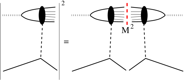
Figure 6: Diagrams relating diffraction with the two-scattering contribution to the total cross section.

The first correction to the non-additivity of cross sections comes from the second-order rescattering $\sigma_{A}^{2}$. In Fig. 7 diffractive DIS is shown both in the infinite momentum frame and in the rest frame of the nucleon. From Fig. 6 it becomes clear that the square of such contribution is equivalent to a double exchange with a cut between the exchanged amplitudes, a so-called diffractive cut. To compute the first contribution to nuclear shadowing $\sigma_{A}^{2}$ which comes from these two exchanges, one needs its total contribution to the $\gamma^{*}$-nucleon cross section. This contribution arises from cutting the two-exchange amplitude in all possible ways: between the amplitudes and the amplitudes themselves in all possible manners. For purely imaginary amplitudes, it can be shown [72, 73] that this total contribution is identical to minus the contribution from the diffractive cut. Thus diffractive DIS is directly related to the first contribution to nuclear shadowing. The final expression reads

$$\sigma_{A}^{2}=-4\pi A(A-1)\int d^{2}b\ T_{A}^{2}(b)\int_{M^{2}_{min}}^{M^{2}_{max}}dM^{2}\left.\frac{d\sigma^{\mathcal{D}}_{\gamma^{*}-{\rm p}}}{dM^{2}dt}\right|_{t=0}F_{A}^{2}(t_{min}),$$ (13)

with $M^{2}$ the mass of the diffractively produced system, $M^{2}_{min}\simeq 4m_{\pi}^{2}$ and $M^{2}_{max}=Q^{2}\left(x_{Pmax}/x-1\right)$ with $x_{Pmax}\sim 0.1$, see [48]. The usual variables for diffractive DIS: $Q^{2}$, $x$, $M^{2}$ and $t$, or $x_{P}=x/\beta$, $\beta=Q^{2}/(Q^{2}+M^{2})$, are shown in Fig. 7.

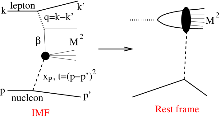
Figure 7: Diffractive dissociation in the infinite momentum frame (IMF), with the corresponding kinematical variables, and in the rest frame of the hadron.

$d\sigma^{\mathcal{D}}_{\gamma^{*}-{\rm p}}/dM^{2}dt$ is the differential cross section for diffractive dissociation of the virtual photon. Coherence effects are taken into account through

$$F_{A}(t_{min})=\int d^{2}b\ J_{0}(b\sqrt{-t_{min}})T_{A}(b),$$ (14)

with $t_{min}=-m_{\rm nucleon}^{2}x_{P}^{2}$. This function is equal to 1 at $x\to 0$ and decreases with increasing $x$ due to the loss of coherence for $x\gtrsim(2m_{\rm nucleon}R_{A})^{-1}$, see (10). Details can be found in the corresponding references [42, 43, 44, 45, 46, 47, 48].

The differences between available realizations come from the consideration of real parts in the pomeron amplitude [46, 47], or from the model or parametrization used for the diffractive cross section: phenomenological models and parametrizations [45, 46, 47, 48] which reproduce the existing experimental data, or a model which considers the evolution of a diffractive $q\bar{q}$ state in [42, 43, 44] (see the method in [76]). Differences also come from the extension of the models to include higher order rescatterings. Such extensions are model-dependent. Some models consider that all intermediate states in the subsequent rescatterings have the same structure [45, 46, 47, 48], in the form of a Schwimmer [77]

$$\sigma^{Sch}_{\gamma^{*}-A}=\sigma_{\gamma^{*}-{\rm nucleon}}\int d^{2}b\,\frac{AT_{A}(b)}{1+(A-1)f(x,Q^{2})T_{A}(b)}$$ (15)

or an eikonal unitarized cross section

$$\sigma^{eik}_{\gamma^{*}-A}=\sigma_{\gamma^{*}-{\rm nucleon}}\int d^{2}b\,\frac{A\left\{1-\exp{\left[-2(A-1)T_{A}(b)f(x,Q^{2})\right]}\right\}}{2(A-1)f(x,Q^{2})}$$ (16)

(with $f(x,Q^{2})$ defined to get consistency with (13) when these equations are expanded to second order). Other models take into account the possibility of different intermediate states [42, 43, 44].

Several comments are in order. First, once the model or parametrization for the diffractive cross section is provided, the extension to the nuclear case is parameter-free - except for the modeling of higher order rescatterings (15) and (16). These models, together with those in Subsection 2.1, provide an impact parameter dependence of nuclear shadowing. In this way, this approach and the one presented in the previous Subsection offer a link between the nucleon and nuclear cases. Second, these models can be used as initial conditions for DGLAP evolution as done in [46, 47], see the next Section. Third, both models for the diffractive cross section and their extension to the nuclear case [45, 48] do not correspond to any definite order in a power expansion in $1/Q$ but perform a re-summation of all powers. Finally, in these models the comparison with experimental data, when such comparison is available, turns out to be reasonable, see Fig. 8 - although the $Q^{2}$-dependence of the nuclear ratios results too smooth compared to data [7], which apparently indicates the need of additional DGLAP evolution.

Figure 8: $x$-dependence of the nuclear $F_{2}$-ratios in the model in [48] for different nuclei, compared with experimental data [8, 9] (circles). Solid lines correspond to Schwimmer (15) and dashed lines to eikonal (16) unitarization. Error bars in the experimental points follow the same convention as in Fig. 5. In the ratios Xe/D, filled circles correspond to the analysis with hadron requirement and open circles to that with electromagnetic cuts, see the experimental paper [8] for more details. Both the experimental results and the theoretical ones, joined by lines, correspond to different average $Q^{2}$ for every different value of $x$. [Figure taken from [48].]

2.3 High-density QCD

High-density QCD - the domain of large gluon densities - has become a very fashionable subject in the last fifteen years. It deals with the behaviour of QCD at very large energies. Regarding the contents of this review, it offers a definite theoretical framework to compute shadowing corrections although the high-energy approximations involved make its applicability to the present experimental situation a subject of intense debate. The literature on this matter is vast and I will not cite but a few papers, referring the reader to the contributions in [19] and to the recent reviews [78, 79, 80, 81] where all the relevant references can be found.

In high-density QCD the small $x$ partons (slow gluons) are treated classically due to the high occupation number $\propto 1/\alpha_{s}$. This number is as high as it can be - thus this field is often referred to as saturation physics. The source term for the classical equations of motion comes from the fast partons e.g. valence quarks with large $x$ (see Fig. 9). The gluon density per unit impact parameter and transverse momentum of the gluon, the so-called unintegrated gluon density at fixed impact parameter, computed in this way for an ultra-relativistic large nucleus - the McLerran-Venugopalan (MV) model [82, 83, 84] - reads

$${dN^{A}_{g}\over dy\,d^{2}b\,d^{2}k_{T}}\equiv{d(xg_{A})\over d^{2}b\,d^{2}k_{T}}\propto{1\over\alpha_{s}}\int{d^{2}x_{T}\over x_{T}^{2}}\,e^{-ix_{T}\cdot k_{T}}\left(1-e^{-x_{T}^{2}Q_{s}^{2}/4}\right).$$ (17)

$Q_{s}^{2}\propto AT_{A}(b)xg_{\rm nucleon}$ is the squared saturation momentum or saturation scale, which corresponds to the typical gluon transverse momentum and to the scale at which the exponential in (17) starts to give large corrections. This saturation scale increases with increasing nuclear size and increasing energy or decreasing $x$. So it is plausible that at some given high energy, $\alpha_{s}$ becomes small enough for perturbative methods to be applied reliably.

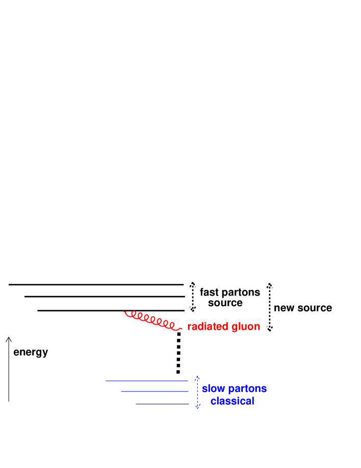
Figure 9: Diagram showing the separation between fast and slow partons, and the contribution from radiated gluons.

With increasing energy, radiation processes start to contribute, see Fig. 9. Additional gluons are radiated from the source in a kinematical region intermediate between the fast and slow ones, and are absorbed in a redefinition of the source. Mathematically this procedure results in a renormalization group equation for the distribution of colour sources in the hadron. Under several simplifications, this renormalization group equation gives a single closed non-linear equation for the dipole-hadron scattering amplitude, the Balitsky-Kovchegov (BK) equation [85, 86]. The use of the dipole model, see Subsection 2.1, provides its link with the nuclear structure functions. Note that in the MV model, the number of partons is not modified but they are only redistributed in transverse momentum, while non-linear BK evolution does diminish the number of gluons.

From the explicit form of the MV model (17), it is obvious that it corresponds to a Glauber-like re-summation of rescatterings in the totally coherent, high-energy limit. Indeed, the MV model can be used as initial condition at some not too small $x\sim 0.01$ for evolution towards smaller $x$ through the BK equation. Other initial conditions have been essayed in the literature. But it is a noticeable property of the BK equation that all initial conditions result in a universal form for the solution of the equation after large enough evolution [87, 88]. Such scaling implies, through the dipole model, that virtual photon-nucleon cross sections are not a function of $x$, $Q^{2}$ and nuclear size separately, but only of $Q^{2}/Q_{s}^{2}$ where all dependence on $x$ and nuclear size is included in $Q_{s}$. This scaling has been found in leptoproduction data on nucleon and nuclear targets [89, 90, 91]. Nevertheless the situation is not yet clear: numerical solutions [92, 93] of the BK equation show that the asymptotic scaling behaviour appears at rapidities larger than those presently available, which are still dominated by the initial conditions. Besides the effects of a running coupling, not included in the derivation of the equation, are large.

Predictions [94, 95, 96] for nuclear structure functions of large nuclei at very small $x$ have been computed in this framework. Some of them are presented in Fig. 10.

Figure 10: Plot on the left: $F_{2}$ for Pb at small $x$ for different $Q^{2}$ computed [95] through the BK equation and the dipole model. Plot on the right: nuclear dependence $\alpha$, $F_{2}^{A}(x,Q^{2})=A^{\alpha(x,Q^{2})}F_{2}^{A=1}(x,Q^{2})$ versus $x$ for different $Q^{2}$. [Figures taken from [95].]

As the main results in this approach, the nuclear structure function at very small $x$ increases as $\ln^{2}{x}$ with decreasing $x$. It also shows a $Q^{2}$-dependence weaker than $\propto Q^{2}$ and a very strong nuclear dependence, with $\alpha(x,Q^{2})$ ($F_{2}^{A}(x,Q^{2})=A^{\alpha(x,Q^{2})}F_{2}^{A=1}(x,Q^{2})$) getting smaller than the geometrical 2/3 factor for very small values of $x$ . Different realizations [94, 95, 96] differ in the initial conditions, in the consideration of impact parameter, and in the treatment of large-size dipoles and of the evolution for not very small $x$. They turn out to give results which may vary as much as a factor 10 for $x\sim 10^{-7}$. Predictions for heavy flavour production also exist [95, 97].

The saturation scale computed within BK evolution behaves like $Q_{s}^{2}\propto x^{-d\alpha_{s}}$, with $d=4\div 5$. Its dependence on the nuclear size is not yet fully determined; in the most widely employed approximation valid for a very large nucleus, the $A$-dependence follows that of the initial conditions, usually $\propto A^{1/3}$. Besides, running coupling effects modify both dependencies dramatically [93]. The saturation scale can also be studied within phenomenological approaches [41, 67, 89, 90, 91]. For example, a value for the saturation scale can be obtained from Glauber approaches (11) as the value of $Q^{2}$ for which the effect of the exponential factor in this equation becomes sizable (other geometrical criteria have also been essayed, like percolation [98]). Values extracted from this kind of studies are $Q_{s}^{2}\sim A^{\delta}(x/0.01)^{-0.3}$ GeV², with $\delta\gtrsim 1/3$.

Finally, other approach to the problem considers power-suppressed corrections in $1/Q$. Such power-suppressed contributions are enhanced by the nuclear size. The first power-suppressed correction to DGLAP evolution [50, 51] results in a non-linear equation. From the equality of the linear and non-linear terms, a value for the saturation scale can be extracted [17] which results in rough agreement with the estimations previously discussed, see the solid black lines in Fig. 3 [17]. More recently, such power-suppressed contributions have been re-summed [54] in the high-energy eikonal limit, resulting in a rescaling of the $x$ variable whose results reasonably describe the experimental data, see Fig. 11. Besides they are in agreement with available data on the nuclear effects on the longitudinal to transverse cross sections [100]. Also more phenomenological studies [55] are in agreement with the experimental data.

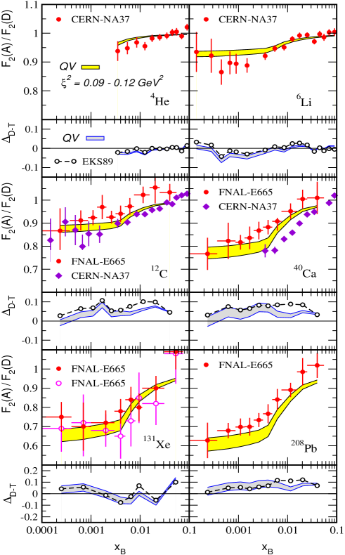
Figure 11: $x$-dependence of the ratios in the model in [54] for different nuclei, compared with experimental data [4, 5, 8, 9] (filled points). The band corresponds to different choices of the scale of power corrections $\xi^{2}$ in [54]. $\Delta_{D-T}={\rm Data}-{\rm Theory}$, and the open circles joined by dashed lines in these plots show the comparison to the approach in [99]. The $(x,Q^{2})$ correlation of the experimental points is taken into account in the theoretical results shown here, as it was in those in Fig. 8. [Figure taken from [54].]

3 Models based on DGLAP evolution

Another type of models do not try to address the origin of nuclear shadowing (or of modifications of parton densities in nuclei in general) but to study the $Q^{2}$-evolution of nuclear ratios of parton densities,

$$R_{i}^{A}(x,Q^{2})={f_{i}^{A}(x,Q^{2})\over A\,f_{i}^{\rm nucleon}(x,Q^{2})}\,,\ \ f_{i}=q,\bar{q},g,$$ (18)

through the DGLAP evolution equations [25, 26, 27], see also [3]. From the very first attempts [101], several analysis have appeared [46, 47, 99, 102, 103, 104, 105, 106]. They try to perform for the nuclear case the same program developed for the nucleon: Nuclear ratios are parametrized at some value $Q_{0}^{2}\sim 1\div 2$ GeV² which is assumed large enough for perturbative DGLAP evolution to be applied reliably. These initial parametrizations for every parton density have to cover the full $x$ range $0<x<1$. In the nuclear case, the nuclear size appears as an additional variable. Then these initial conditions are evolved through the DGLAP equations towards larger values of $Q^{2}$ and compared with experimental data. From this comparison the initial parametrizations are adjusted.

Different approaches differ in several details, see [17]:

• The form of the parametrizations at the initial scale. For example, in [99, 103] shadowing saturates for very small $x$, contrary to [106]. Also the value of $Q_{0}^{2}$ varies e.g. from $\sim 0.4$ GeV² [106] to 2.25 GeV² [99, 103]. The parametrizations for sea quarks and gluons in [104] do not show any EMC effect. Special mention has to be done to the approach of [46, 47] where the initial gluon density is taken from diffractive nucleon data at $Q_{0}^{2}=4$ GeV² as discussed in Subsection 2.2 and no attempt is made to modify it from the comparison with experimental data.

• The use of different sets of experimental data. For example, Drell-Yan data [13] are used in [99, 103, 105, 106] but not in [104]. These data give the main constraint to the valence and sea contributions in the antishadowing region in [99, 103] but the parametrizations in [105] do not show antishadowing for sea quarks. HERMES data [108] are used in [105]. Also the data on the $Q^{2}$-dependence of nuclear ratios [7] are included in [99, 103, 105, 106] but not in [104]; they give the main constrain on the gluon distribution at small and moderate $x$, see below.

• The order of DGLAP evolution. The evolution is made at leading order (LO) in [99, 103] and at next-to-leading (NLO) order in  [104, 105, 106]. This turns out to modify the $Q^{2}$-dependence of nuclear ratios.

• The treatment of isospin effects and the use of sum rules as additional constraints for evolution. For example, isospin symmetry of the nuclear ratios is assumed in [99, 103] but not in [104]. Momentum, charge and baryon number conservation are used in [104, 106], but charge conservation is not used in [99, 103]. In practice, these differences result numerically small.

• The different nucleon partons densities used in the analysis. In practice this choice is of little importance at the level of the nuclear ratios, as its effect appears in both the numerator and denominator in (18) and cancels to a large extent.

A comparison of different approaches can be found in Fig. 12; see also Section 4. The differences are noticeable, even more when one considers that all approaches have been designed to reproduce available experimental data (but see below the discussion on the $Q^{2}$-dependence of nuclear ratios), see [17] for comments. Concerning shadowing, it turns out that the nuclear ratios for gluons are almost unconstrained for $x<0.02$, and for sea quarks for $x<0.005$. The stronger constraint on gluons in the region $0.02<x<0.2$ comes from the $Q^{2}$-dependence of nuclear ratios which I will discuss now.

Figure 12: Nuclear ratios for Ca versus $x$ computed for different partons densities, for two different values of $Q^{2}$. Results from [106] (solid), [99] (dashed) and [104] (dotted lines) are compared. [Figure taken from [106].]

The DGLAP equations establish a relation between the logarithmic $Q^{2}$-evolution of the structure functions and the gluon distribution [109]. Such relation, valid at LO and small $x$, has been extended to the nuclear ratios [110]:

$$\frac{\partial R_{F_{2}}^{A}(x,Q^{2})}{\partial\ln Q^{2}}\approx\frac{10\alpha_{s}}{27\pi}\frac{xg(2x,Q^{2})}{\frac{1}{2}F_{2}^{\rm deuterium}(x,Q^{2})}\biggl{\{}R_{g}^{A}(2x,Q^{2})-R_{F_{2}}^{A}(x,Q^{2})\biggr{\}}.$$ (19)

In this way, $R_{g}^{A}(2x,Q^{2})>R_{F_{2}}^{A}(x,Q^{2})$ implies a positive $Q^{2}$ slope, while $R_{g}^{A}(2x,Q^{2})<R_{F_{2}}^{A}(x,Q^{2})$ gives a negative slope. The available data on the $Q^{2}$-dependence of nuclear ratios [7] allow to constraint within the DGLAP evolution scheme, the relation between the nuclear gluon distribution and the nuclear ratio for $F_{2}$. In Fig. 13 the result of $Q^{2}$-evolution of the nuclear $F_{2}$-ratio for Sn over C is shown [110] for different models [99, 104], and also for DGLAP-evolved parametrizations [111, 112] (these parametrizations were originally proposed as $Q^{2}$-independent). While in the parametrization [112] the ratio for all flavours is equal at the initial scale $Q_{0}^{2}$, and thus it gives a too small but positive slope, in the parametrization of  [111] the shadowing for gluons is much larger than that for sea and valence quarks so it results in a negative slope at the smallest $x$ and $Q^{2}$. Therefore, from the comparison with experimental data [7], DGLAP analysis favours those sets in which gluons are less shadowed than quarks for $x\sim 0.01$. This is at variance with some approaches e.g. [46, 47] where gluons are more shadowed than quarks, see the next Section. As commented in Subsection 2.2, the discrepancy between the data and the results of this model when evolved to smaller values of $Q^{2}$ from $Q_{0}^{2}=4$ GeV² is considered as evidence of the existence of large power-suppressed contributions.

Figure 13: Results of the models [99] (solid) and [104] (dashed-dotted), and of DGLAP evolution of initial conditions from [112] (dashed) and [111] (dotted lines), for the $Q^{2}$-evolution of the ratio Sn/C at different values of $x$, compared with the experimental data [7]. [Figure taken from [110].]

While DGLAP approaches do not address the fundamental problem of the origin of shadowing, they are of great practical interest. They provide the parton densities required to compute cross sections for observables characterized by a hard scale for which collinear factorization [113] can be applied, see Section 5 and [17] for discussions and further references. As a final comment, the centrality dependence of shadowing is not addressed in these models as the existing experimental data do not allow its determination, although some approaches e.g. [111, 114] provide an ansatz for such a dependence.

4 Comparison among different models

In Fig. 14 a comparison of the results of different models for $R_{F_{2}}^{\rm Pb}$ is shown. The results coincide within $\sim 15$ % in the region $x\sim 0.01$ where experimental data exists. But they strongly disagree for smaller values of $x$, the difference being almost a factor 2 at $x\sim 10^{-5}$. In general, models [46, 48] based on Gribov inelastic shadowing give a larger shadowing than those based in Glauber-like rescatterings [40, 41]. The model [96] based on high-density QCD gives less shadowing. Among the models based on DGLAP evolution, [99, 103] gives larger shadowing than [104] and to the one in [106], see Fig. 12 for sea quarks which determine $F_{2}$ for small $x$. But one should take into account that in DGLAP approaches the small $x$ behaviour at $Q^{2}$ close to $Q_{0}^{2}$ comes mainly from the assumptions for the initial conditions. The model [107] gives results for $R_{F_{2}}^{\rm Pb}$ at $Q^{2}=2.25$ GeV² very close to those of [99, 103] at $x=0.01$ where the considered high-density corrections are almost negligible, but sizably smaller, $R_{F_{2}}^{\rm Pb}\simeq 0.43$, at $x=10^{-5}$. These predictions could be checked in the EIC [24], where values of $x\sim 3\cdot 10^{-4}$ at $Q^{2}\sim 1$ GeV² should become accessible, or in ultra-peripheral proton-ion or ion-ion collisions (UPC) [115, 116].

Figure 14: $F_{2}$-ratios for Pb versus $x$ at fixed $Q^{2}=3$ GeV² from the models: Armesto et al. (“this work”) [48], HKM [104], Sarcevic [40], Bartels [96], Frankfurt [46] (at $Q^{2}=4$ GeV²), Armesto [41] and EKS98 [99, 103]. [Figure taken from [48].]

Now let me turn to the nuclear gluon density. In those approaches [40, 41] which rely on the dipole model, the gluon density is obtained from the unintegrated gluon distribution through

$$xg_{A}(x,Q^{2})=\int_{\Lambda^{2}}^{Q^{2}}d^{2}k_{T}\int d^{2}b\,{d(xg_{A})\over d^{2}b\,d^{2}k_{T}}\,,$$ (20)

where $\Lambda^{2}$ is some infrared cut-off, if required. This identification is only true for $Q^{2}\gg Q_{\rm sat}^{2}$ [117, 118, 119]. In models based on Gribov inelastic shadowing [46, 120], the nuclear gluon density is obtained from (13)-(16) but using the gluon density in the pomeron instead of the diffractive structure function of the proton.

In Fig. 15 a comparison of the results of different models for $R_{g}^{\rm Pb}$ is shown. At variance to the case of $R_{F_{2}}^{\rm Pb}$, now there are large discrepancies also at $x\sim 0.01$, see the discussion on the $Q^{2}$-dependence of the nuclear ratios at the end of Section 3. This is due to the fact that the gluon density is only indirectly constrained by experimental data - $F_{2}$ is mainly determined by the sea quarks at such values of $x$. The discrepancy between the different approaches is roughly a factor 2 at $x\sim 0.01$ and a factor 3 at $x\sim 10^{-5}$. Among the DGLAP approaches the results of [111], in which gluon shadowing is fixed to reproduce the multiplicity in Au-Au collisions at RHIC (see the next Section), are clearly below those from [99, 103] and [104], as discussed at the end of Section 3. Again, these DGLAP results are mainly determined by the initial parametrizations. The results of Glauber-like models are similar at $x\sim 10^{-5}$ but those of [41] are smaller than the ones in [40] at $x\sim 0.01$. Results from Gribov inelastic shadowing [46] show a strong shadowing: see Fig. 15 and the mentioned discussion in Section 3; [120] gives $R_{g}^{\rm Pb}\sim 0.7$ at $x=0.01$ and $\sim 0.2$ at $x=10^{-5}$ for $Q^{2}=6.5$ GeV². The model [107] gives results for $R_{g}^{\rm Pb}$ at $Q^{2}=2.25$ GeV² very close to those of [99, 103] at $x=0.01$ - as it was the case for $R_{F_{2}}$, but sizably smaller, $R_{F_{2}}^{\rm Pb}\simeq 0.37$, at $x=10^{-5}$. Finally, [42] gives $R_{g}^{\rm Pb}\sim 0.95$ at $x=0.01$ and $\sim 0.75$ at $x=10^{-4}$ for $Q^{2}=4$ GeV².

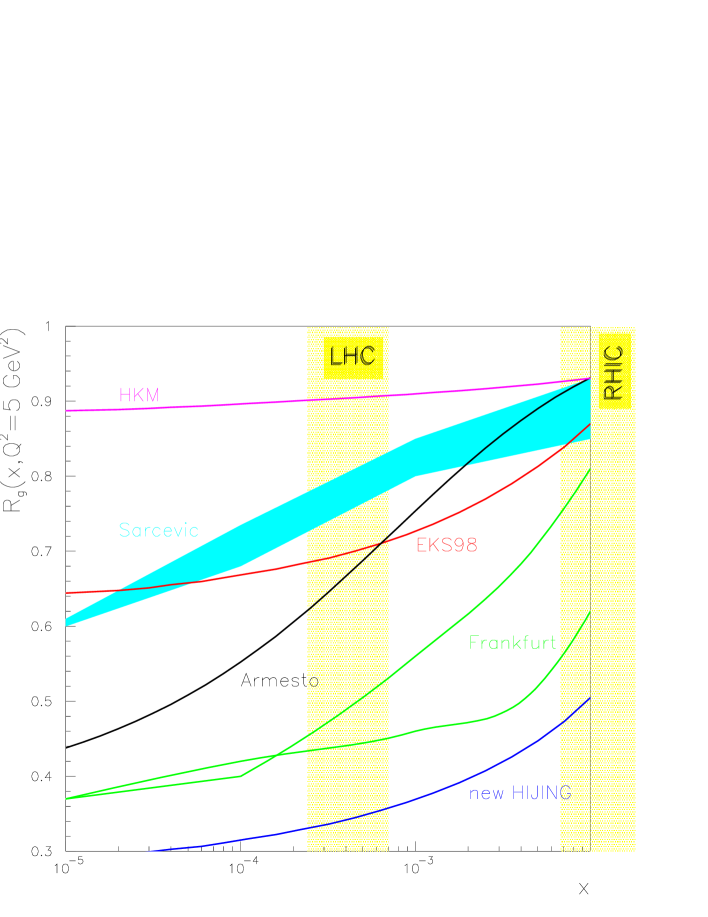
Figure 15: Ratios of gluon distribution functions for Pb versus $x$ from different models at $Q^{2}=5$ GeV²: HKM [104], Sarcevic [40], EKS98 [99, 103], Frankfurt [46], Armesto [41] and new HIJING [111]. RHIC and LHC point the ranges of $x=(Q/\sqrt{s_{{}_{\it{NN}}}})e^{y}$ for processes with $|y|\leq 0.5$, $Q^{2}=5$ GeV² at RHIC ($\sqrt{s_{{}_{\it{NN}}}})=200$ GeV) and LHC ($\sqrt{s_{{}_{\it{NN}}}})=5.5$ TeV) respectively. [Figure taken from [17].]

Contrary to $F_{2}$ which is directly measurable, the gluon distribution is only indirectly constrained both at an EIC [24], in proton-nucleus or nucleus-nucleus collisions at RHIC [20, 21, 22, 23] and the LHC [17], and in UPC [115, 116]. Some of these indirect constraints in proton-nucleus and nucleus-nucleus collisions will be discussed in the next Section.

5 Shadowing and particle production in high-energy nuclear collisions

In this Section I will discuss some consequences of the phenomenon of shadowing in high-energy nuclear collisions. I will devote most of the Section to proton(deuteron)-nucleus collisions, and only at the end I will briefly refer to nucleus-nucleus collisions.

Particle production is related to the parton densities in the projectile and target through a factorization theorem, which in general takes the schematic form

$$\sigma_{A-B\to CX}\propto\phi_{i/A}(x_{A})\otimes\phi_{j/B}(x_{B})\otimes\hat{\sigma}_{ij\to C}(x_{A},x_{B},Q_{C}).$$ (21)

In this formula, integration over the relevant variable is implicit. $\hat{\sigma}$ is a scattering matrix for partons $i,j$ to give the produced parton/particle $C$. $Q_{C}$ is a scale (e.g. mass, transverse momentum,$\dots$) characteristic of $C$. And $\phi_{i/A}(x_{A})$ are the probabilities of finding parton $i$ in hadron/nucleus $A$ with momentum fraction $x_{A}$. Depending on the type of factorization, collinear for $\Lambda_{\rm QCD}\ll Q_{C}\ll\sqrt{s}$ [113] or $k_{T}$ for $\Lambda_{\rm QCD}\ll Q_{C}\lesssim\sqrt{s}$ [121, 122, 123], the matrix elements are different and the partons distributions are integrated or unintegrated respectively [119]. For the status of collinear factorization in collisions involving nuclei, see [17]. The validity and exact form of $k_{T}$ factorization in proton-nucleus collisions - here proton means a hadron in which the parton density is small - is under discussion, see e.g. [124, 125, 126] and references therein. For nucleus-nucleus [129, 130, 131], arguments exist which indicate that it is not valid [132, 133], but the size of the violations has not been fully quantified yet. Therefore, most of the discussions in the literature assume the validity of such factorizations in the nuclear case, which will be done in the following.

In a $2\to 2$ process the relation between rapidity $y$ and transverse mass $m_{T}=\sqrt{m^{2}+p_{T}^{2}}$ of the final partons/particles and their fractional momenta $x_{A,B}$ is

$$x_{A,B}={m_{T}\over\sqrt{s}}\,\exp{(\pm y)}.$$ (22)

At midrapidity at RHIC, only particle production with small $p_{T}\lesssim 1\div 2$ GeV will be sensitive to the shadowing region in parton densities. At the LHC, the region of transverse momenta will be much larger, see Fig. 3 for the relevant kinematical regions which will be studied in proton-nucleus collisions at RHIC and the LHC for different observables. In [17] extensive studies of the impact of parton densities on particle production with a large scale (e.g. transverse momentum or mass) at the LHC can be found.

Most of the discussions at RHIC are done in terms of the so-called nuclear modification factors:

$$R_{A-B}={{\rm produced\ in}\ A-B\over{\rm expected\ in}\ A-B}={N_{A-B}\over N_{coll}\times N_{\rm nucleon-nucleon}}\,.$$ (23)

Here $N_{A-B}$ is the number of produced particles of a given type in some kinematical region, in $A$-$B$ collisions. $N_{coll}$ is the number of binary incoherent nucleon-nucleon collisions with which particle production is expected to scale in collinear factorization, so $R_{A-B}\to 1$ for a large scale of the produced particle.

In Fig. 16 the nuclear modification factor for neutral pion production in d-Au collisions at RHIC for pseudorapidity $\eta\simeq 0$ is shown and compared with results from collinear factorization [106]. Nuclear effects in deuterium, as stated previously, are usually neglected and, in any case, very small. From this Figure it becomes clear that at midrapidities only the region of small transverse momentum ($p_{T}\lesssim 1$ GeV) is sensitive to the amount of shadowing in parton densities. Above $p_{T}\sim 3$ GeV, one can see a (small) enhancement of particle production in nuclear targets - a phenomenon known as the Cronin effect for more than 20 years [135].

Figure 16: Nuclear modification factor for neutral pions at $\eta\simeq 0$ in d-Au collisions at $\sqrt{s_{{}_{\it{NN}}}}=200$ GeV. The curves are the results from [106] and the experimental data from [134]. [Figure taken from [106].]

A large quark mass also provides a scale which gives some justification to the use of collinear factorization. Thus heavy flavour production can be employed to constrain parton densities inside nuclei [136, 137] and their impact parameter dependence [138]. At RHIC, direct measurements of open heavy flavour production are still at the beginning [139]. Most of the existing data are obtained from electrons from semi-leptonic decays [140, 141] which are weakly correlated with the parent heavy flavour. On the other hand, there exist studies of charmonium production. In Fig. 17 results for J/$\psi$ production in d-Au collisions at RHIC [142] for different pseudorapidities are shown and compared [143] to models for partons densities, using collinear factorization. Such models imply for forward rapidities, see (22), an additional suppression (i.e. gluon shadowing as heavy flavour production is mostly sensitive to the gluon channel) on top of the nuclear absorption of quarkonium in nuclei [144, 145]. From Fig. 17 right, models which do not consider a very strong gluon shadowing [99, 103] are apparently favoured over those which consider a large shadowing [46], see also the discussion at the end of Section 3. But the large error bars in the experimental data and the remaining uncertainty in the amount of nuclear absorption and its behaviour with rapidity [63, 64], make it difficult to extract any definite conclusion.

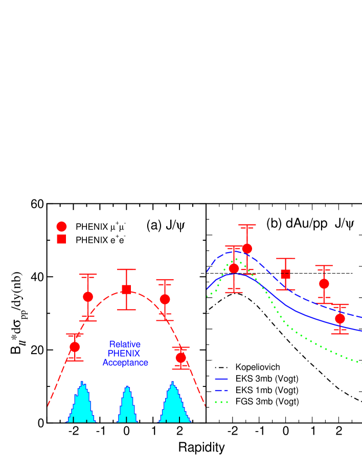
Figure 17: Plot on the left: rapidity distribution of the J/$\psi$ cross section. Plot on the right: nuclear modification factor for J/$\psi$ [142] in d-Au collisions at $\sqrt{s_{{}_{\it{NN}}}}=200$ GeV. The curves in this plot labeled Vogt [143] correspond to different nuclear absorption cross sections and different models for nuclear parton densities EKS [99, 103] and FGS [46], while that labeled Kopeliovich corresponds to [64]. [Figure taken from [142].]

A striking finding in d-Au collisions at RHIC has been the change from an enhancement of the nuclear modification factor for light particles at central pseudorapidities (the Cronin effect, see Fig. 16) to a suppression, at all measured transverse momenta, at forward pseudorapidities [14, 15, 146, 147] (Fig. 18), see the review [148]. In Glauber-like models as the MV model, the Cronin effect results naturally from the transverse momentum broadening due to multiple scattering. But it has been taken as a great success of saturation physics that non-linear small-$x$ evolution was able to predict the suppression at all transverse momentum from initial conditions which contained the Cronin effect [92, 149, 150, 151]. Studies within collinear factorization [152] indicate that shadowing has to be stronger than usually considered in DGLAP or Gribov inelastic shadowing [153] approaches, in order to justify these forward data, and that other effects are at work. In any case the clear conclusion can be drawn that such data require a large amount of shadowing, even more considering that the average values of $x$ probed in the nucleus are not very small, $\langle x\rangle\sim 0.01$ (assuming $2\to 2$ processes) [152]. Other observables like Drell-Yan production [17, 154, 155, 156, 157], and midrapidity production of high-$p_{T}$ hadrons in proton-nucleus collisions at the LHC, should further clarify this issue.

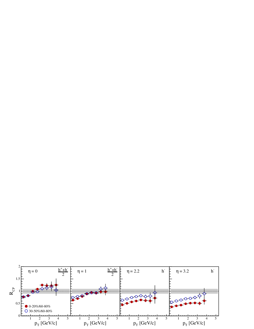
Figure 18: Ratio of nuclear modification factors for different centrality classes, for charged (two leftmost plots) and negative (two rightmost plots) particles at different pseudorapidities for central/peripheral (filled points) and semicentral/peripheral (open points) d-Au collisions at $\sqrt{s_{{}_{\it{NN}}}}=200$ GeV [14]. [Figure taken from [14].]

d-Au collisions at RHIC have been crucial to establish the baseline on top of which final state effects due to a new state of deconfined matter, the Quark Gluon Plasma, can be searched for and eventually characterized [158]. Due to this possibility, the determination of nuclear shadowing in nucleus-nucleus collisions is far more complex than in proton-nucleus, as many other effects can be at work. In any case, the influence of shadowing on bulk particle production will be large, resulting in a strong reduction of multiplicities in Au-Au collisions at RHIC and Pb-Pb collisions at the LHC, see e.g. the reviews [159, 160], or [130, 131, 161]. For example, in the approach [48] based on Gribov inelastic shadowing and assuming some kind of factorization based on the AGK rules, reduction factors in head-on heavy ion collisions $\sim 2$ at RHIC and $\sim 4$ at the LHC can be expected for particle production at mid-rapidity, compared to $p$-$p$ collisions scaled by the number of binary collisions. Other approaches [91] based on saturation ideas which directly relate the shadowing measured in lepton-nucleus collisions to multiplicities in proton-nucleus and nucleus-nucleus collisions, also predict large suppressions and result in agreement with experimental data, see Fig. 19. Nevertheless it must be stressed that the uncertainties on the separation of effects in the nuclear wave functions from other effects due to the collision are large, as there is no well established factorization scheme presently available for nucleus-nucleus collisions.

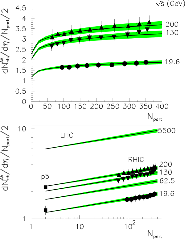
Figure 19: Energy and centrality dependence (in terms of the number $N_{\rm part}$ of nucleons participating in the collision) of the multiplicity of charged particles at midrapidity divided by $N_{\rm part}$, in Au-Au collisions at several RHIC energies and for LHC energies. The results [91] of $(2/N_{\rm part})[dN^{A-A}_{\rm ch}/d\eta](\eta\sim 0)=0.47[\sqrt{s_{{}_{\it{NN}}}}]^{0.288}N_{\rm part}^{0.089}$ are compared to PHOBOS data [162, 163]. Also shown in the lower panel are the ${\bar{p}}$-$p$ data [164, 165], as quoted in [163]. [Figure taken from [91].]

6 Conclusions

The phenomenon of shadowing is of large importance from a theoretical point of view: the behaviour of the nuclear wave function at high energies provides useful information for our understanding of QCD in such regime. It has also very strong practical implications: parton densities in nuclei are required to predict and understand particle production in collisions involving nuclei. In this article the phenomenon of nuclear shadowing has been introduced. I have discussed multiple scattering as the underlying physical mechanism illustrated through a simple example of two scatterings, and presented several models which make use of it. Then I have analyzed the DGLAP approach which does not address the origin of shadowing but only the evolution of nuclear parton densities through the DGLAP equations. Next I have shown a comparison of the different models for $F_{2}$ and $xg$. Finally, I have reviewed the results in nuclear collisions for which shadowing is expected to play a large role, with special emphasis on proton(deuteron)-nucleus collisions at RHIC.

The uncertainties on gluon shadowing at small $x\lesssim 10^{-2}$ are as large as a factor 3, see Fig. 15. Multiple scattering approaches suggest a large amount of shadowing and tend to indicate that shadowing for gluons is stronger than that for quarks. But DGLAP evolution disfavours such situation in view of the existing data on $Q^{2}$-evolution of the nuclear modification factors, at least for $x\sim 0.01$ where experimental data lie. In this $x$-region the uncertainties in multiple scattering approaches are large due to finite coherence length effects. Besides, at the existing values of $Q^{2}$ for small $x$ the validity of pure DGLAP evolution or the need of power-suppressed corrections, re-summed in the totally coherent limit in some approaches like high-density QCD, is not yet clear. So more data at smaller $x$, eventually coming from a large energy lepton-nucleus collider like the EIC [24], or from UPC [115, 116], are needed.

d-Au collisions at RHIC provide very useful information if the validity of some form of factorization is assumed. J/$\psi$ production data in the forward (deuteron) direction constrain, within collinear factorization, shadowing for gluons, apparently favouring models with not very large shadowing. On the other hand, nuclear modification factors for charged or negative particles in the forward direction show a suppression for all transverse momenta first predicted in the framework of high-density QCD. They seem to indicate that shadowing has to be larger than in most available models. Both sets of experimental data truly imply more physical mechanisms than nuclear shadowing, and some sizable uncertainty still comes from the use of any kind of factorization.

Nucleus-nucleus collisions at RHIC and the LHC will be strongly affected by shadowing. Thus, the quantification of shadowing effects will be crucial for the eventual characterization of a dense medium where many additional physical processes may be at work. In this respect, in the near future the LHC will open new possibilities, both with the heavy ion program and, mainly, with proton-nucleus runs [17].

References

References

- [1] Arneodo M 1994 Phys. Rept. 240 301
- [2] Geesaman D F, Saito K and Thomas A W 1995 Ann. Rev. Nucl. Part. Sci. 45 337
- [3] Roberts R G 1990 The structure of the proton (Cambridge University Press)
- [4] Amaudruz P et al. [New Muon Collaboration] 1995 Nucl. Phys. B 441 3
- [5] Arneodo M et al. [New Muon Collaboration] 1995 Nucl. Phys. B 441 12
- [6] Arneodo M et al. [New Muon Collaboration] 1996 Nucl. Phys. B 481 3
- [7] Arneodo M et al. [New Muon Collaboration] 1996 Nucl. Phys. B 481 23
- [8] Adams M R et al. [E665 Collaboration] 1992 Phys. Rev. Lett.68 3266
- [9] Adams M R et al. [E665 Collaboration] 1995 Z. Phys. C 67 403
- [10] Arnold R G et al. [E139 Collaboration] 1984 Phys. Rev. Lett.52 727
- [11] Arneodo M et al. [European Muon Collaboration] 1988 Phys. Lett.B 211 493
- [12] Arneodo M et al. [European Muon Collaboration] 1990 Nucl. Phys.B 333 1
- [13] Alde D M et al. [E772 Collaboration] 1990 Phys. Rev. Lett.64 2479
- [14] Arsene I et al. [BRAHMS Collaboration] 2004 Phys. Rev. Lett.93 242303
- [15] Adler S S et al. [PHENIX Collaboration] 2005 Phys. Rev. Lett.94 082302
- [16] d’Enterria D 2004 J. Phys. G 30 S767 [Erratum-ibid. G31 283]
- [17] Accardi A et al. 2004 CERN Yellow Report on Hard probes in Heavy-Ion Collisions at the LHC (CERN-2004-009), Chapter 1: pdf’s, shadowing and pA collisions (Geneva: CERN Scientific Information Service) (Preprint hep-ph/0308248)
- [18] Brodsky S J, Close F E and Gunion J F 1972 Phys. Rev.D 6 177
- [19] Blaizot J-P and Iancu E (eds) 2002 QCD Perspectives on Hot and Dense Matter (NATO Science Series II: Mathematics, Physics and Chemistry vol. 87) (Kluwer Academic Publishers)
- [20] Adcox K et al. [PHENIX Collaboration] 2005 Nucl. Phys. A 757 184
- [21] Back B B et al. [PHOBOS Collaboration] 2005 Nucl. Phys. A 757 28
- [22] Arsene I et al. [BRAHMS Collaboration] 2005 Nucl. Phys. A 757 1
- [23] Adams J et al. [STAR Collaboration] 2005 Nucl. Phys. A 757 102
- [24] Deshpande A, Milner R, Venugopalan R and Vogelsang W 2005 Ann. Rev. Nucl. Part. Sci. 55 165
- [25] Dokshitzer Y L 1977 Sov. Phys. JETP 46 641
- [26] Gribov V N and Lipatov L N 1972 Sov. J. Nucl. Phys. 15 438
- [27] Altarelli G and Parisi G 1977 Nucl. Phys.B 126 298
- [28] Stodolsky L 1967 Phys. Rev. Lett.18 135
- [29] Schildknecht D 1973 Nucl. Phys.B 66 398
- [30] Nikolaev N N and Zakharov V I 1975 Phys. Lett.B 55 397
- [31] Shaw G 1989 Phys. Lett.B 228 125
- [32] Kulagin S A, Piller G and Weise W 1994 Phys. Rev.C 50 1154
- [33] Kwiecinski J and Badelek B 1988 Phys. Lett.B 208 508
- [34] Frankfurt L L and Strikman M I 1989 Nucl. Phys.B 316 340
- [35] Brodsky S J and Lu H J 1990 Phys. Rev. Lett.64 1342
- [36] Nikolaev N N and Zakharov B G 1991 Z. Phys. C 49 607
- [37] Barone V, Genovese M, Nikolaev N N, Predazzi E and Zakharov B G 1993 Z. Phys. C 58 541
- [38] Kopeliovich B Z and Povh B 1996 Phys. Lett.B 367 329
- [39] Armesto N and Braun M A 1997 Z. Phys. C 76 81
- [40] Huang Z, Lu H J and Sarcevic I 1998 Nucl. Phys.A 637 79
- [41] Armesto N 2002 Eur. Phys. J. C 26 35
- [42] Kopeliovich B Z, Schäfer A and Tarasov A V 2000 Phys. Rev.D 62 054022
- [43] Kopeliovich B Z, Raufeisen J and Tarasov A V 2000 Phys. Rev.C 62 035204
- [44] Nemchik J 2003 Phys. Rev.C 68 035206
- [45] Capella A, Kaidalov A B, Merino C, Pertermann D and Tran Thanh Van J 1998 Eur. Phys. J. C 5 111
- [46] Frankfurt L L, Guzey V, McDermott M and Strikman M I 2002 JHEP 0202 027
- [47] Frankfurt L L, Guzey V and Strikman M I 2005 Phys. Rev.D 71 054001
- [48] Armesto N, Capella A, Kaidalov A B, Lopez-Albacete J and Salgado C A 2003 Eur. Phys. J. C 29 531
- [49] Gribov L V, Levin E M and Ryskin M G 1983 Phys. Rept. 100 1
- [50] Mueller A H and Qiu J W 1986 Nucl. Phys.B 268 427
- [51] Qiu J W 1987 Nucl. Phys.B 291 746
- [52] Berger E L and Qiu J W 1988 Phys. Lett.B 206 141
- [53] Close F E and Roberts R G 1988 Phys. Lett.B 213 91
- [54] Qiu J W and Vitev I 2004 Phys. Rev. Lett.93 262301
- [55] Castorina P 2005 Phys. Rev.D 72 097503
- [56] Smirnov G I 1995 Phys. Lett.B 364 87
- [57] Glauber R J 1959 Lectures in Theoretical Physics vol 1 ed W E Brittin et al. (New York: Interscience) p 315
- [58] Gribov V N 1969 Sov. Phys. JETP 29 483
- [59] Gribov V N 1970 Sov. Phys. JETP 30 709
- [60] Hebecker A 2000 Phys. Rept. 331 1
- [61] Klein S 1999 Rev. Mod. Phys.71 1501
- [62] Baier R, Schiff D and Zakharov B G 2000 Ann. Rev. Nucl. Part. Sci. 50 37
- [63] Braun M A, Pajares C, Salgado C A, Armesto N and Capella A 1998 Nucl. Phys.B 509 357
- [64] Kopeliovich B Z, Tarasov A and Hufner J 2001 Nucl. Phys.A 696 669
- [65] Mueller A H 1994 Nucl. Phys.B 415 373
- [66] Mueller A H and Patel B 1994 Nucl. Phys.B 425 471
- [67] Golec-Biernat K and Wusthoff M 1999 Phys. Rev.D 59 014017
- [68] Kuraev E A, Lipatov L N and Fadin V S 1977 Sov. Phys. JETP 45 199
- [69] Balitsky I I and Lipatov L N 1978 Sov. J. Nucl. Phys. 28 822
- [70] Frankfurt L L, Radyushkin A and Strikman M I 1997 Phys. Rev.D 55 98
- [71] Goncalves V P and Machado M V T 2004 Eur. Phys. J. C 38 319
- [72] Gribov V N 1968 Sov. Phys. JETP 26 414
- [73] Abramovsky V A, Gribov V N and Kancheli O V 1974 Sov. J. Nucl. Phys. 18 308
- [74] Bartels J, Salvadore M and Vacca G P 2005 Eur. Phys. J. C 42 53
- [75] Collins J C 1998 Phys. Rev.D 57 3051 [Erratum 2000 Phys. Rev.D 61 019902]
- [76] Zakharov B G 1998 Phys. Atom. Nucl. 61 838
- [77] Schwimmer A 1975 Nucl. Phys.B 94 445
- [78] Iancu E and Venugopalan R 2003 Quark Gluon Plasma 3 ed R C Hwa and X N Wang (World Scientific) p 249 (Preprint hep-ph/0303204)
- [79] McLerran L D 2005 Nucl. Phys.A 752 355
- [80] Kovner A 2005 Acta Phys. Polon. B 36 3551
- [81] Triantafyllopoulos D N 2005 Acta Phys. Polon. B 36 3593
- [82] McLerran L D and Venugopalan R 1994 Phys. Rev.D 49 2233
- [83] McLerran L D and Venugopalan R 1994 Phys. Rev.D 49 3352
- [84] McLerran L D and Venugopalan R 1994 Phys. Rev.D 50 2225
- [85] Balitsky I I 1996 Nucl. Phys.B 463 99
- [86] Kovchegov Y V 1999 Phys. Rev.D 60 034008
- [87] Armesto N and Braun M A 2001 Eur. Phys. J. C 20 517
- [88] Lublinsky M 2001 Eur. Phys. J. C 21 513
- [89] Stasto A M, Golec-Biernat K and Kwiecinski J 2001 Phys. Rev. Lett.86 596
- [90] Freund A, Rummukainen K, Weigert H and Schafer A 2003 Phys. Rev. Lett.90 222002
- [91] Armesto N, Salgado C A and Wiedemann U A 2005 Phys. Rev. Lett.94 022002
- [92] Albacete J L, Armesto N, Kovner A, Salgado C A and Wiedemann U A 2004 Phys. Rev. Lett.92 082001
- [93] Albacete J L, Armesto N, Milhano J G, Salgado C A and Wiedemann U A 2005 Phys. Rev.D 71 014003
- [94] Levin E and Lublinsky M 2001 Nucl. Phys.A 696 833
- [95] Armesto N and Braun M A 2001 Eur. Phys. J. C 22 351
- [96] Bartels J, Gotsman J, Levin E M, Lublinsky M and Maor U 2003 Phys. Rev.D 68 054008
- [97] Goncalves V P and Machado M V T 2003 Eur. Phys. J. C 30 387
- [98] Armesto N and Salgado C A 2001 Phys. Lett.B 520 124
- [99] Eskola K J, Kolhinen V J and Salgado C A 1999 Eur. Phys. J. C 9 61
- [100] Abe K et al. [E143 Collaboration] 1999 Phys. Lett.B 452 194
- [101] Eskola K J 1993 Nucl. Phys.B 400 240
- [102] Indumathi D and Zhu W 1997 Z. Phys. C 74 119
- [103] Eskola K J, Kolhinen V J and Ruuskanen P V 1998 Nucl. Phys.B 535 351
- [104] Hirai M, Kumano S and Miyama M 2001 Phys. Rev.D 64 034003
- [105] Hirai M, Kumano S and Nagai T H 2004 Phys. Rev.C 70 044905
- [106] de Florian D and Sassot R 2004 Phys. Rev.D 69 074028
- [107] Ayala Filho A L and Goncalves V P 2001 Eur. Phys. J. C 20 343
- [108] Ackerstaff K et al. [HERMES Collaboration] 2000 Phys. Lett.B 475 386 [Erratum-ibid. B 567 339]
- [109] Prytz K 1993 Phys. Lett.B 311 286
- [110] Eskola K J, Honkanen H, Kolhinen V J and Salgado C A 2002 Phys. Lett.B 532 222
- [111] Li S y and Wang X N 2002 Phys. Lett.B 527 85
- [112] Czyzewski J, Eskola K J and Qiu J W 1995 III International Workshop on Hard Probes of Dense Matter (ECT*, Trento, June 1995)
- [113] Collins J C, Soper D E and Sterman G 1988 Adv. Ser. Direct. High Energy Phys. 5 1
- [114] Emel’yanov V, Khodinov A, Klein S R and Vogt R 2000 Phys. Rev.C 61 044904
- [115] Bertulani C A, Klein S R and Nystrand J 2005 Ann. Rev. Nucl. Part. Sci. 55 271
- [116] Gonçalves V P and Machado M V T 2006 Phys. Rev.C 73 044902
- [117] Kovchegov Y V and Mueller A H 1998 Nucl. Phys.B 529 451
- [118] Mueller A H 1999 Nucl. Phys.B 558 285
- [119] Collins J C 2003 Acta Phys. Polon. B 34 3103
- [120] Tywoniuk K, Arsene I C, Bravina L, Kaidalov A B and Zabrodin E 2005 (Preprint hep-ph/0510371)
- [121] Catani S, Ciafaloni M and Hautmann F 1991 Nucl. Phys.B 366 135
- [122] Collins J C and Ellis R K 1991 Nucl. Phys.B 360 3
- [123] Levin E M, Ryskin M G, Shabelski Y M and Shuvaev A G 1991 Sov. J. Nucl. Phys. 53 657
- [124] Braun M A 2006 (Preprint hep-ph/0603060)
- [125] Kovchegov Y V and Tuchin K 2002 Phys. Rev.D 65 074026
- [126] Nikolaev N N, Schafer W and Zakharov B G 2005 Phys. Rev. Lett.95 221803
- [127] Nikolaev N N , Schafer W and Schwiete G 2001 Phys. Rev.D 63 014020
- [128] Nikolaev N N and Schafer W 2005 Phys. Rev.D 71 014023
- [129] Braun M A 2000 Phys. Lett.B 483 105
- [130] Kharzeev D E and Nardi M 2001 Phys. Lett.B 507 121
- [131] Kharzeev D E and Levin E M 2001 Phys. Lett.B 523 79
- [132] Balitsky I I 2004 Phys. Rev.D 70 114030
- [133] Fujii H, Gelis F and Venugopalan R 2005 Phys. Rev. Lett.95 162002
- [134] Adler S S et al. [PHENIX Collaboration] 2003 Phys. Rev. Lett.91 072303
- [135] Cronin J W et al. 1975 Phys. Rev.D 11 3105
- [136] Armesto N, Pajares C, Salgado C A and Shabelski Y M 1996 Phys. Lett.B 366 276
- [137] Armesto N, Pajares C, Salgado C A and Shabelski Y M 1998 Phys. Atom. Nucl. 61 125
- [138] Klein S R and Vogt R 2003 Phys. Rev. Lett.91 142301
- [139] Tai A et al. [STAR Collaboration] 2004 J. Phys. G 30 S809
- [140] Adler S S et al. [PHENIX Collaboration] 2006 Phys. Rev. Lett.96 032301
- [141] Bielcik J et al. [STAR Collaboration] 2005 (Preprint nucl-ex/0511005)
- [142] Adler S S et al. [PHENIX Collaboration] 2006 Phys. Rev. Lett.96 012304
- [143] Vogt R 2005 Phys. Rev.C 71 054902
- [144] Capella A, Casado J A, Pajares C, Ramallo A V and Tran Thanh Van J 1988 Phys. Lett.B 206 354
- [145] Gerschel C and Hufner J 1988 Phys. Lett.B 207 253
- [146] Back B B et al. [PHOBOS Collaboration] 2004 Phys. Rev.C 70 061901
- [147] Adams J et al. [STAR Collaboration] 2006 (Preprint nucl-ex/0602011)
- [148] Jalilian-Marian J and Kovchegov Y V 2006 Prog. Part. Nucl. Phys. 56 104
- [149] Kharzeev D E, Levin E M and McLerran L D 2003 Phys. Lett.B 561 93
- [150] Baier R, Kovner A and Wiedemann U A 2003 Phys. Rev.D 68 054009
- [151] Kharzeev D E, Kovchegov Y V and Tuchin K 2003 Phys. Rev.D 68 094013
- [152] Guzey V, Strikman M and Vogelsang W 2004 Phys. Lett.B 603 173
- [153] Capella A, Ferreiro E G, Kaidalov A B and Sousa D 2005 Eur. Phys. J. C 40 129
- [154] Kopeliovich B Z, Raufeisen J, Tarasov A V and Johnson M B 2003 Phys. Rev.C 67 014903
- [155] Gelis F and Jalilian-Marian J 2002 Phys. Rev.D 66 094014
- [156] Baier R, Mueller A H and Schiff D 2004 Nucl. Phys.A 741 358
- [157] Betemps M A and Gay Ducati M B 2004 Phys. Rev.D 70 116005
- [158] Gyulassy M and McLerran L D 2005 Nucl. Phys.A 750 30
- [159] Armesto N and Pajares C 2000 Int. J. Mod. Phys. A 15 2019
- [160] Armesto N 2005 J. Phys. Conf. Ser. 5 219
- [161] Braun M A and Pajares C 2006 (Preprint hep-ph/0603184)
- [162] Back B B et al. [PHOBOS Collaboration] 2002 Phys. Rev.C 65 061901
- [163] Back B B et al. [PHOBOS Collaboration] 2004 Phys. Rev.C 70 021902
- [164] Thome W et al. [Aachen-CERN-Heidelberg-Munich Collaboration] 1977 Nucl. Phys.B 129 365
- [165] Alner G J et al. [UA5 Collaboration] 1986 Z. Phys. C 33 1