HD-THEP-04-18

IFUM-790-FT

ECT^∗-05-19

hep-ph/0604087

Towards a Nonperturbative Foundation
of the Dipole Picture:
II. High Energy Limit

Carlo Ewerz ^a,b,c,1, Otto Nachtmann ^a,2

^a Institut für Theoretische Physik, Universität Heidelberg
Philosophenweg 16, D-69120 Heidelberg, Germany

^b Dipartimento di Fisica, Università di Milano and INFN, Sezione di Milano
Via Celoria 16, I-20133 Milano, Italy

^c ECT ^∗, Strada delle Tabarelle 286, I-38050 Villazzano (Trento), Italy

This is the second of two papers in which we study real and virtual photon-proton scattering in a nonperturbative framework. In the first paper we have identified the leading contributions to this process at high energies and have derived expressions for them which take into account the renormalisation of the photon-quark-antiquark vertex. In the present paper we investigate the approximations and assumptions that are necessary to obtain the dipole model of high energy scattering from the results derived in the first paper. We discuss the gauge invariance of different contributions to the scattering amplitude and point out some subtleties related to gauge invariance in the correct definition of a perturbative photon wave function. As a phenomenological consequence of the dipole picture we derive a bound on the ratio of the cross sections for longitudinally and transversely polarised photons. This bound is independent of any particular model for the dipole-proton cross section and allows one to test the validity of the assumptions leading to the dipole picture in particular at low photon virtualities. We conclude that the naive dipole model formula should be supplemented by two additional terms which can potentially become large at small photon virtualities.

  ¹ email: Ewerz@ect.it
² email: O.Nachtmann@thphys.uni-heidelberg.de

1 Introduction

In this paper we continue our study of real and virtual photon-proton scattering in a nonperturbative framework which we have initiated in [1], hereafter referred to as I. Sections of that paper will be referred to as I.2.1 and equations as (I.1) etc. We use the same notation and conventions as in I, and definitions made there will not be repeated here. In the present paper we include only references that are directly relevant to the material treated here, for a more extensive list of references we refer the reader to I.

In the first paper we have classified the contributions to the process of real or virtual photon-proton scattering, see section I.2.1, figure I.2. We have identified the leading contributions at high energies in sect. I.2.2 and have derived expressions for them which take into account the renormalisation of the photon-quark-antiquark vertex. In the present paper we study in detail the high energy limit. We investigate the approximations and assumptions that are necessary to derive the dipole model of high energy scattering from the results obtained in the first paper. We point out that the naive dipole model formula should be supplemented by two additional terms which can potentially become large at small photon virtualities.

Gauge invariance is known to place strong constraints on current-induced scattering amplitudes. We find it therefore interesting to study the gauge invariance of different contributions to the scattering amplitude. It turns out that at finite energies the part of the Compton amplitude from which the dipole picture emerges is not gauge invariant separately. This also leads to subtleties in the definition of the wave function of longitudinally polarised photons which we discuss in some detail.

As a key result of the present paper we identify the assumptions and approximations that lead us from the most general description of the Compton amplitude to the usual dipole picture. We consider it a very important task to test the validity of those assumptions and approximations for the experimentally accessible ranges of the kinematic variables. In the dipole picture the total photon-proton cross section is a convolution of the square of the photon wave function with the reduced cross section describing the scattering of a colour dipole off the proton. At present, the reduced cross section cannot be derived from first principles and one has to retreat to models based on ideas like saturation. One finds that the currently available data permit considerable freedom for models of the reduced cross section. If one is to find phenomenological tests of the dipole picture (and hence of the assumptions on which it is based) one should thus concentrate on the other convolution factor in the dipole formula, that is on the photon wave function. This motivates us to study in some detail the properties of the wave function.

As an immediate consequence of the dipole formula for the total virtual photon-proton cross section we derive a bound on the ratio $R$ of the cross sections for longitudinally and transversely polarised photons that results only from the respective photon wave functions. Although there are only few data points available at energies sufficiently high for one reasonably to expect the dipole model to be applicable the bound turns out to give some indication as to the photon virtualities below which the dipole model becomes questionable. In this region the two additional terms mentioned above should become relevant.

In the dipole picture one talks about a quark-antiquark pair scattering on a target. If we want to be rigorous we have to face the question how far we can go treating quarks as asymptotic states. Of course, quarks are confined and do not have a mass shell. In this paper we shall nevertheless assume – as is usually done – that we can treat quarks and antiquarks as asymptotic particles. As we shall show we can then make a precise connection between the photon induced reaction and the reaction where the photon is replaced by a superposition of quark-antiquark states. We leave the investigation of the realistic case of quarks which have no mass shell for future work. At present we may give the following simple argument. Let us assume that the two-point functions for quarks have a Källen-Lehmann representation with standard properties, but with no mass shell. This is indicated by calculations using lattice as well as Schwinger-Dyson equation methods, see for example [2]. We can then think that the mass-distribution function of a quark propagator may have a strong peak at some value $m_{q}$ which we shall call the quark mass. If the peak is approximated by a $\delta$-function we have effectively a quark mass shell.

This second paper is organised as follows. We start by discussing the high energy limit of the parts of the Compton amplitude that are leading at high energies and identify their asymptotic behaviour in section 2. In section 3 we investigate the separate gauge invariance of different parts of the amplitude. The derivation of the photon wave function is performed in section 4 where we also discuss the gauge non-invariance of this object and its consequences for the choice of the photon polarisation vectors. In section 5 we generalise our findings to the case of more general amplitudes with incoming and outgoing photons and define dipole states. In section 6 we finally obtain the usual dipole picture and identify all underlying assumptions and approximations. Here we also study the properties of the photon wave function. In section 7 we derive a bound on the ratio of the cross sections for longitudinally and transversely polarised virtual photons that needs to be satisfied if the usual dipole picture is valid, and compare this bound to the available experimental data. Our conclusions are presented in section 8. In appendix A we collect some technical details relevant to the discussion of the high energy limit in sections 2 and 4. Appendix B supplements section 3 with further discussion of the separate gauge invariance of different parts of the Compton amplitude which are subleading at high energies.

2 The high energy limit

In this section we shall study the high energy limit of the real or virtual Compton amplitude (I.LABEL:2.3), $|\mathbf{q}|\rightarrow\infty$ with $Q^{2}$ fixed. Our aim is to obtain eventually the usual dipole picture of high energy photon-proton scattering. As was discussed in section I.LABEL:sec:relsize in the high energy limit the two amplitudes $\mathcal{M}^{(a)}$ and $\mathcal{M}^{(b)}$ give the leading contribution to the full amplitude. However, it is only the amplitude $\mathcal{M}^{(a)}$ from which we expect the usual dipole picture to emerge. In the present section we will therefore study mainly that amplitude $\mathcal{M}^{(a)}$ (I.LABEL:2.8), (I.LABEL:2.20). But it should be kept in mind that at low photon virtuality an important correction to the dipole picture can arise from the amplitude $\mathcal{M}^{(b)}$, see the discussion in section I.LABEL:sec:relsize.

We will mainly be concerned here with the term $\mathcal{M}^{(a,1)}$ (I.LABEL:2.33) of $\mathcal{M}^{(a)}$ which we will find to be leading in the high energy limit, whereas the terms $\mathcal{M}^{(a,2)}$ to $\mathcal{M}^{(a,4)}$ are subleading. In the amplitude $\mathcal{M}^{(a,1)}$ by definition only the momentum $k^{\prime(1)}$ occurs but not the momenta $k^{\prime(2)}$ to $k^{\prime(4)}$ which correspond to the other three parts of amplitude $\mathcal{M}^{(a)}$, see (I.LABEL:B.20)-(I.LABEL:B.23). Therefore we now simplify our notation and write $k^{\prime}$ instead of $k^{\prime(1)}$ and $\mathbf{k}^{\prime}$ instead of $\mathbf{k}^{\prime(1)}$.

Let us now consider the term $\mathcal{M}^{(a,1)}$ which we have obtained in (I.LABEL:2.33) in the form

$$\mathcal{M}^{(a,1)\mu\nu}_{s^{\prime}s}(p^{\prime},p,q)\! = \!\frac{1}{2\pi}\sum_{q}Q^{2}_{q}\int\frac{d\omega}{\omega+i\epsilon}\int\frac{d^{3}k}{(2\pi)^{3}2k^{0}}(q^{0}-k^{0}-k^{\prime 0}-\omega+i\epsilon)^{-1}$$

$${}(2k^{\prime 0})^{-1}\sum_{r^{\prime},r}\langle\gamma(q^{\prime},\mu),p(p^{\prime},s^{\prime})|\mathcal{T}^{(a)}|\bar{q}(k^{\prime}_{\omega},r^{\prime}),q(k_{\omega},r),p(p,s)\rangle$$

$${}\bar{u}_{r}(k)\left\{\Gamma^{(q)\nu}(k,-k^{\prime})+\sum_{q^{\prime}}\int K^{(q,q^{\prime})}S^{(q^{\prime})}_{F}\Gamma^{(q^{\prime})\nu}S^{(q^{\prime})}_{F}\right\}v_{r^{\prime}}(k^{\prime})\,,$$

and let us in particular concentrate on the integration over $\omega$ in the complex $\omega$-plane. Recall that $\omega$ is the off-shell part of the energy of the quark on the left-hand side of the diagram in figure I.LABEL:fig4a, see (I.LABEL:B.3). We expect the matrix element of $\mathcal{T}^{(a)}$ to be regular in the vicinity of $\omega=0$. Thus we have the two explicit pole factors in the integrand (2) with the poles in $\omega$ situated at $\omega=-i\epsilon$ and at $\omega=-\Delta E+i\epsilon$ with

$$\Delta E=k^{0}+k^{\prime 0}-q^{0}\,,$$ (2)

see figure 1.

Figure 1: The singularities of the integrand of $\mathcal{M}^{(a,1)}$ (2) in the $\omega$-plane. There are poles at $\omega=-i\epsilon$ and $\omega=-\Delta E+i\epsilon$.

One finds that always $\Delta E>0$. The poles will contribute a factor of order $1/q^{0}$ in the amplitude unless there is a pinching of the two singularities, that is for

$$-\Delta E=q^{0}-k^{0}-k^{\prime 0}\rightarrow 0\,.$$ (3)

The conditions for this to happen are easily derived and in principle well known. To make the article self-contained we discuss them here in detail. We have from (I.LABEL:B.20)

$$\mathbf{q}-\mathbf{k}-\mathbf{k}^{\prime} = 0\,,$$

$$q^{0} = \sqrt{\mathbf{q}^{2}-Q^{2}}$$

$$k^{0} = \sqrt{\mathbf{k}^{2}+m^{2}_{q}}\,,$$

$$k^{\prime 0} = \sqrt{\mathbf{k}^{\prime 2}+m^{2}_{q}}\,.$$ (4)

We set

$$\mathbf{k} = \alpha\mathbf{q}+\mathbf{k}_{T},$$

$$\mathbf{k}^{\prime} = (1-\alpha)\mathbf{q}-\mathbf{k}_{T}\,,$$ (5)

where we suppose

$$\mathbf{q}\,\mathbf{k}_{T}=0\,,$$ (6)

that is, longitudinal and transverse directions are defined relative to $\mathbf{q}$. We then get

$$\Delta E = {}(q^{0}+k^{0}+k^{\prime 0})^{-1}\left[(k^{0}+k^{\prime 0})^{2}-(q^{0})^{2}\right]$$ (7)

$$= {}(q^{0}+k^{0}+k^{\prime 0})^{-1}\left[Q^{2}+2m^{2}_{q}+2k^{0}k^{\prime 0}-2\mathbf{k}\,\mathbf{k}^{\prime}\right]$$

$$= {}2(q^{0}+k^{0}+k^{\prime 0})^{-1}\bigg{[}\,\frac{1}{2}\,Q^{2}+(\alpha^{2}\mathbf{q}^{2}+\mathbf{k}^{2}_{T}+m^{2}_{q})^{1/2}$$

$${}\left((1-\alpha)^{2}\mathbf{q}^{2}+\mathbf{k}^{2}_{T}+m^{2}_{q}\right)^{1/2}-\alpha(1-\alpha)\mathbf{q}^{2}+\mathbf{k}^{2}_{T}+m_{q}^{2}\bigg{]}\,.$$

For large $|\mathbf{q}|$ the energy difference $\Delta E$ becomes small only if the terms proportional to $\mathbf{q}^{2}$ in the square brackets cancel. This happens for $\alpha\neq 0,1$ if and only if

$$|\alpha(1-\alpha)|-\alpha(1-\alpha)=0\,,$$ (8)

that is for

$$0<\alpha<1\,.$$ (9)

Thus we get a pinch and a large contribution only if the splitting of the photon $q$ is into a quark-antiquark pair where the longitudinal momenta are both in the direction $\mathbf{q}$. Note again that we have used no arguments related to perturbation theory to arrive at this conclusion.

We can rewrite (7) in yet another form:

$$\Delta E=\frac{Q^{2}+\tilde{m}^{2}(\alpha,\mathbf{k}_{T})}{q^{0}+k^{0}+k^{\prime 0}}\,,$$ (10)

where

$$\tilde{m}^{2}(\alpha,\mathbf{k}_{T})=2(\mathbf{k}^{2}_{T}+m^{2}_{q})$$ (11)

$$\left[\,1+\frac{\left(\alpha^{2}+(1-\alpha)^{2}\right)\mathbf{q}^{2}+\mathbf{k}^{2}_{T}+m^{2}_{q}}{(\alpha^{2}\mathbf{q}^{2}+\mathbf{k}^{2}_{T}+m^{2}_{q})^{\frac{1}{2}}\left((1-\alpha)^{2}\mathbf{q}^{2}+\mathbf{k}^{2}_{T}+m^{2}_{q}\right)^{\frac{1}{2}}+\alpha(1-\alpha)\mathbf{q}^{2}}\right].$$

In figure 2 we show the range in $\mathbf{k}^{2}_{T}+m^{2}_{q}$ corresponding to

$$\tilde{m}^{2}(\alpha,\mathbf{k}_{T})\leq\bar{Q}^{2}\,,$$ (12)

where $\bar{Q}$ is some chosen fixed mass scale for which we always suppose $\bar{Q}^{2}\geq 4m^{2}_{q}$ and $0\leq\alpha\leq 1$.

Figure 2: The upper limit of k${}^{2}_{T}+m^{2}_{q}$ corresponding to $\tilde{m}^{2}(\alpha,$k${}_{T})\leq\bar{Q}^{2}$ (see (13), (14)).

We see that (12) corresponds to

$$\mathbf{k}^{2}_{T}+m^{2}_{q}\,\leq\,\frac{\bar{Q}^{4}}{4(\mathbf{q}^{2}+\bar{Q}^{2})}$$ (13)

for $\alpha=0$ and $\alpha=1$ , and to

$$\mathbf{k}_{T}^{2}+m^{2}_{q}\,\leq\,\frac{1}{4}\bar{Q}^{2}$$ (14)

for $\alpha=1/2$. Thus the pinch condition in the form

$$\Delta E\leq\frac{Q^{2}+\bar{Q}^{2}}{q^{0}+k^{0}+k^{\prime 0}}$$ (15)

is only fulfilled for $\alpha\rightarrow 0$ and $1$ for very small $\mathbf{k}^{2}_{T}+m^{2}_{q}$ whereas for $\alpha\approx 1/2\quad\mathbf{k}^{2}_{T}+m^{2}_{q}$ ranges up to $\mathcal{O}(\bar{Q}^{2})$. This is discussed in more detail in appendix A.1.

Taking now only the contribution from the pinch in (2) we obtain asymptotically for large $|\mathbf{q}|$

$$\mathcal{M}^{(a,1)\mu\nu}_{s^{\prime}s}(p^{\prime},p,q) = i\sum_{q}Q^{2}_{q}\int\frac{d^{3}k}{(2\pi)^{3}2k^{0}2k^{\prime 0}}\,(\Delta E)^{-1}\,\theta\left(\bar{Q}^{2}-\tilde{m}^{2}(\alpha,\mathbf{k}_{T})\right)$$

$${}\sum_{r^{\prime},r}\,\langle\gamma(q^{\prime},\mu),p(p^{\prime},s^{\prime})|\mathcal{T}^{(a)}|\bar{q}(k^{\prime},r^{\prime}),q(k,r),p(p,s)\rangle$$

$${}\bar{u}_{r}(k)\left\{\Gamma^{(q)\nu}(k,-k^{\prime})+\sum_{q^{\prime}}\int K^{(q,q^{\prime})}S^{(q^{\prime})}_{F}\Gamma^{(q^{\prime})\nu}S^{(q^{\prime})}_{F}\right\}v_{r^{\prime}}(k^{\prime})\,.$$

Here the four-momenta $k,k^{\prime}$ are given as in (2) and (2) with $0\leq\alpha\leq 1$. We have inserted a $\theta$-function to ensure the pinch condition in the form (15). This limits $\mathbf{k}^{2}_{T}$ as shown in figure 2; see also the discussion in appendix A.1.

We note that in $\mathcal{M}^{(a,2)}$ to $\mathcal{M}^{(a,4)}$, (I.LABEL:2.23)-(I.LABEL:2.25), no pinch of the explicit pole terms in $\omega$ occurs and we expect these terms to be suppressed relative to the leading term (2) by a factor of the order

$$\frac{\Delta E}{q^{0}}\approx\frac{Q^{2}+\bar{Q}^{2}}{(q^{0})^{2}}$$ (17)

for large $|\mathbf{q}|$.

In (2) we already see something like the dipole picture emerging. The photon splits into a $q\bar{q}$ pair with both the quark and the antiquark on the mass shell $m_{q}$. This on-shell pair interacts with the proton to produce the final state. But the photon ‘wave function’ is not simply the vertex function. There is also the piece containing the kernel $K^{(q,q^{\prime})}$ which in a way represents rescattering corrections of the $q\bar{q}$-pair.

We should keep in mind also the contribution from the amplitude $\mathcal{M}^{(b)}$. In complete analogy to the discussion above we start from (I.LABEL:2.45) and find a pinch singularity also for that amplitude. The leading term in $\mathcal{M}^{(b)}$ for large $|\mathbf{q}|$ then asymptotically becomes

$$\mathcal{M}^{(b,1)\mu\nu}_{s^{\prime}s}(p^{\prime},p,q) = i\sum_{q^{\prime\prime},q}Q_{q^{\prime\prime}}Q_{q}\int\frac{d^{3}k}{(2\pi)^{3}2k^{0}2k^{\prime 0}}\,(\Delta E)^{-1}\,\theta\left(\bar{Q}^{2}-\tilde{m}^{2}(\alpha,\mathbf{k}_{T})\right)$$

$${}\sum_{r^{\prime},r}\,\langle\gamma(q^{\prime},\mu),p(p^{\prime},s^{\prime})|\mathcal{T}^{(q^{\prime\prime},b)}|\bar{q}(k^{\prime},r^{\prime}),q(k,r),p(p,s)\rangle$$

$${}\bar{u}_{r}(k)\left\{\Gamma^{(q)\nu}(k,-k^{\prime})+\sum_{q^{\prime}}\int K^{(q,q^{\prime})}S^{(q^{\prime})}_{F}\Gamma^{(q^{\prime})\nu}S^{(q^{\prime})}_{F}\right\}v_{r^{\prime}}(k^{\prime})\,.$$

The discussion of the high energy limit presented here is consistent with the well-known space-time picture of photon-hadron scattering at high energies that is the origin of the dipole picture. The quantity $\Delta E$ is the energy imbalance between the photon and the quark-antiquark pair, see (2). According to the energy-time uncertainty relation the quark-antiquark pair into which the photon fluctuates can therefore live at most for a time $(\Delta E)^{-1}$. In the high energy limit we have $\Delta E\to 0$ (for fixed $Q^{2}$) such that the maximal lifetime of the pair increases with increasing energy. In the rest frame of the proton, for example, the photon typically splits into the quark-antiquark pair already at a large distance from the proton. The actual interaction of the pair with the proton then takes place on much shorter timescales. Some typical values of $\Delta E$ in realistic situations are given in appendix A.

In order to extract the dipole picture explicitly from the formulae obtained above it will turn out to be useful to address first the problem of gauge invariance of various parts of the amplitude.

3 Gauge invariance

In this section we want to study the question of electromagnetic gauge invariance of the real or virtual Compton amplitude. In particular we are interested in the question whether the different parts of the amplitude arising from the decompositions that we have performed up to this point are separately gauge invariant. In the following we will therefore consider the general amplitude without imposing the high energy limit. Only in section 3.3 we will come back to this limit.

The full Compton amplitude (I.LABEL:2.3) obviously exhibits electromagnetic gauge invariance. More precisely, electromagnetic current conservation implies

$$q_{\nu}\mathcal{M}^{\mu\nu}_{s^{\prime}s}(p^{\prime},p,q)=0\,.$$ (19)

Here and in the following we always consider current conservation for the incoming photon, hence the contraction with $q_{\nu}$. The outgoing photon can be treated analogously.

3.1 Skeleton decomposition of the full amplitude

We first consider the general decomposition of the amplitude derived in section I.LABEL:nonpertsect and do not yet impose the high energy limit.

Again we are in particular interested in the contributions $\mathcal{M}^{(a)}$ and $\mathcal{M}^{(b)}$ represented by figures I.LABEL:fig2a and I.LABEL:fig2b, which are not suppressed at high energies. Let us first consider the contribution $\mathcal{M}^{(a)}$, that is the term from which the usual dipole picture emerges at high energies, as we will see in the following sections.

We start from expression (I.LABEL:2.8) in which we recognise that the $q$-dependence of $\mathcal{M}^{(a)}$ is fully contained in the term $A^{(q)\mu\nu}(q)$ given in (I.LABEL:2.8a). We therefore consider the expression

$$q_{\nu}A^{(q)\mu\nu}(q) = \int d^{4}x\,\left(q_{\nu}e^{-iqx}\right)\mathrm{Tr}\left[\gamma^{\mu}S_{F}^{(q)}(0,x;G)\gamma^{\nu}S_{F}^{(q)}(x,0;G)\right]$$ (20)

$$= {}\int d^{4}x\,\left(i\frac{\partial}{\partial x^{\nu}}\,e^{-iqx}\right)\mathrm{Tr}\left[\gamma^{\mu}S_{F}^{(q)}(0,x;G)\gamma^{\nu}S_{F}^{(q)}(x,0;G)\right]$$

$$= {}-\int d^{4}x\,e^{-iqx}\,i\frac{\partial}{\partial x^{\nu}}\mathrm{Tr}\left[\gamma^{\mu}S_{F}^{(q)}(0,x;G)\gamma^{\nu}S_{F}^{(q)}(x,0;G)\right]\,,$$

where we have integrated by parts. This contains the following expression, in which we can complete the derivatives to full covariant derivatives in order to obtain inverse quark propagators,

$$i\frac{\partial}{\partial x^{\nu}}\mathrm{Tr}\left[\gamma^{\mu}S_{F}^{(q)}(0,x;G)\gamma^{\nu}S_{F}^{(q)}(x,0;G)\right]$$ (21)

$$= {}\mathrm{Tr}\left[\gamma^{\mu}S_{F}^{(q)}(0,x;G)\left(i\!\stackrel{{\scriptstyle\leftarrow}}{{\!\not\!\partial}}_{x}+i\!\stackrel{{\scriptstyle\rightarrow}}{{\!\not\!\partial}}_{x}\right)S_{F}^{(q)}(x,0;G)\right]$$

$$= {}\mathrm{Tr}\left\{\gamma^{\mu}S_{F}^{(q)}(0,x;G)\left[\left(i\!\stackrel{{\scriptstyle\leftarrow}}{{\not\!\!D}}_{x}+m_{q}^{(0)}\right)+\left(i\!\stackrel{{\scriptstyle\rightarrow}}{{\not\!\!D}}_{x}-m_{q}^{(0)}\right)\right]S_{F}^{(q)}(x,0;G)\right\}\,.$$

Inserting this back in (20) we obtain with (I.LABEL:A.4) and (I.LABEL:A.4b)

$$q_{\nu}A^{(q)\mu\nu}(q) = -\int d^{4}x\,e^{-iqx}\,\mathrm{Tr}\left[\gamma^{\mu}\delta^{(4)}(x)S_{F}^{(q)}(x,0;G)-\gamma^{\mu}\delta^{(4)}(x)S_{F}^{(q)}(0,x;G)\right]$$ (22)

$$= 0\,.$$

Consequently, the amplitude $\mathcal{M}^{(a)}$ is separately gauge invariant,

$$q_{\nu}\mathcal{M}^{(a)\mu\nu}_{s^{\prime}s}(p^{\prime},p,q)=0\,.$$ (23)

Next we turn to the amplitude $\mathcal{M}^{(b)}$. The factor in that amplitude which is relevant for our considerations here is according to (I.LABEL:Mbexpl) given by $A_{b}^{(q)\nu}(q)$, see (I.LABEL:C.3). Its contraction with $q_{\nu}$ gives

$$q_{\nu}A_{b}^{(q)\nu}(q) = q_{\nu}\int d^{4}x\,e^{-iqx}\,\mathrm{Tr}\left[\gamma^{\nu}S_{F}^{(q)}(x,x;G)\right]$$ (24)

$$= {}-\int d^{4}x\,e^{-iqx}\,i\frac{\partial}{\partial x^{\nu}}\mathrm{Tr}\left[\gamma^{\nu}S_{F}^{(q)}(x,x;G)\right]\,,$$

where we have again integrated by parts. The derivative of the trace then becomes

$$i\frac{\partial}{\partial x^{\nu}}\mathrm{Tr}\left[\gamma^{\nu}S_{F}^{(q)}(x,x;G)\right] = \mathrm{Tr}\left[i\!\stackrel{{\scriptstyle\rightarrow}}{{\!\not\!\partial}}_{x}S_{F}^{(q)}(x,x;G)\right]$$ (25)

$$= {}\left.\mathrm{Tr}\left[i\!\stackrel{{\scriptstyle\rightarrow}}{{\!\not\!\partial}}_{x}S_{F}^{(q)}(x,x^{\prime};G)+S_{F}^{(q)}(x,x^{\prime};G)i\!\stackrel{{\scriptstyle\leftarrow}}{{\!\not\!\partial}}_{x^{\prime}}\right]\right|_{x^{\prime}=x}$$

Here we can again complete full covariant derivatives and obtain for (24) with (I.LABEL:A.4) and (I.LABEL:A.4b)

$$q_{\nu}A_{b}^{(q)\nu}(q) = -\int d^{4}x\,e^{-iqx}\,\mathrm{Tr}\left[\left(i\!\stackrel{{\scriptstyle\rightarrow}}{{\not\!\!D}}_{x}-m_{q}^{(0)}\right)S_{F}^{(q)}(x,x^{\prime};G)\right.$$ (26)

$${}\hskip 85.35826pt\left.+\,S_{F}^{(q)}(x,x^{\prime};G)\left.\left(i\!\stackrel{{\scriptstyle\leftarrow}}{{\not\!\!D}}_{x^{\prime}}+m_{q}^{(0)}\right)\right]\right|_{x^{\prime}=x}$$

$$= {}\left.\int d^{4}x\,e^{-iqx}\,\mathrm{Tr}\left[\delta^{(4)}(x-x^{\prime})-\delta^{(4)}(x-x^{\prime})\right]\right|_{x^{\prime}=x}$$

$$= {}0\,.$$

Hence also the amplitude $\mathcal{M}^{(b)}$ is separately gauge invariant,

$$q_{\nu}\mathcal{M}^{(b)\mu\nu}_{s^{\prime}s}(p^{\prime},p,q)=0\,.$$ (27)

Finally we consider the remaining parts of the amplitude in the skeleton decomposition, $\mathcal{M}^{(c)}$ – $\mathcal{M}^{(g)}$, which are subleading in the high energy limit. Here we find that $\mathcal{M}^{(c)}$ taken together with $\mathcal{M}^{(d)}$ is gauge invariant,

$$q_{\nu}\left(\mathcal{M}^{(c)\mu\nu}_{s^{\prime}s}(p^{\prime},p,q)+\mathcal{M}^{(d)\mu\nu}_{s^{\prime}s}(p^{\prime},p,q)\right)=0\,,$$ (28)

whereas each of the remaining three amplitudes $\mathcal{M}^{(e)}$, $\mathcal{M}^{(f)}$ and $\mathcal{M}^{(g)}$ is gauge invariant by itself,

$$q_{\nu}\mathcal{M}^{(e)\mu\nu}_{s^{\prime}s}(p^{\prime},p,q)=q_{\nu}\mathcal{M}^{(f)\mu\nu}_{s^{\prime}s}(p^{\prime},p,q)=q_{\nu}\mathcal{M}^{(g)\mu\nu}_{s^{\prime}s}(p^{\prime},p,q)=0\,.$$ (29)

The derivation of these results is presented in appendix B.

3.2 Decomposition of the amplitudes ${\cal M}^{(a)}$ and ${\cal M}^{(b)}$

Among the contributions to the skeleton decomposition of the full amplitude we have identified $\mathcal{M}^{(a)}$ and $\mathcal{M}^{(b)}$ as the ones that will be leading at high energies. We now turn to the spin sum decomposition which we have performed for these two amplitudes. At this point we still consider the general decomposition of these amplitudes performed before taking the high energy limit.

We have decomposed $\mathcal{M}^{(a)}$ into the four terms $\mathcal{M}^{(a,j)}$, $j=1,\dots,4$, see (I.LABEL:2.20)-(I.LABEL:2.25) and the graphical illustration in figure I.LABEL:fig4. According to (23) we clearly have

$$q_{\nu}\sum_{j=1}^{4}\mathcal{M}^{(a,j)\mu\nu}_{s^{\prime}s}(p^{\prime},p,q)=0\,.$$ (30)

Since we have obtained the dipole picture only from $\mathcal{M}^{(a,1)}$, it is now interesting to see whether that part is gauge invariant by itself. We use the expression (2) for $\mathcal{M}^{(a,1)}$ and remember that the terms in curly brackets in that equation equal $Z_{q}\gamma^{\nu}$ via (I.LABEL:2.31). Hence the contraction $q_{\nu}\mathcal{M}^{(a,1)\mu\nu}_{s^{\prime}s}(p^{\prime},p,q)$ contains as the relevant factor in the integrand the expression

$$q_{\nu}\bar{u}_{r}(k)Z_{q}\gamma^{\nu}v_{r^{\prime}}(k^{\prime}) = Z_{q}\bar{u}_{r}(k)\!\not\!q\,v_{r^{\prime}}(k^{\prime})$$ (31)

$$= {}Z_{q}\bar{u}_{r}(k)\left[(\not\!k-m_{q})+(\not\!k^{\prime}+m_{q})-(\Delta E)\gamma^{0}\right]v_{r^{\prime}}(k^{\prime})$$

$$= {}-(\Delta E)Z_{q}\bar{u}_{r}(k)\gamma^{0}v_{r^{\prime}}(k^{\prime})\,,$$

where we have used (2), (2), and that by definition the spinors $u$ and $v$ are solutions of the free Dirac equation,

$$\bar{u}_{r}(k)(\not\!k-m_{q}) = {}0\,,$$

$$(\not\!k^{\prime}+m_{q})v_{r^{\prime}}(k^{\prime}) = {}0\,.$$ (32)

Clearly, (31) is in general different from zero. Inserting that term back into the full expression (2) for $\mathcal{M}^{(a,1)}$ we thus find that the resulting expression does in general not vanish. Hence the amplitude $\mathcal{M}^{(a,1)}$ does in general not fulfil electromagnetic gauge invariance separately.

Similar considerations hold for each of the other three terms $\mathcal{M}^{(a,j)}$, $j=2,3,4$, in (I.LABEL:2.20). None of them is gauge invariant separately.

The situation for the spin sum decomposition (I.LABEL:C.11) of the amplitude ${\cal M}^{(b)}$ into the terms ${\cal M}^{(b,j)}$ ($j=1,\dots,4$) is completely analogous. None of the terms ${\cal M}^{(b,j)}$ given in (I.LABEL:C.13) - (I.LABEL:C.16) is gauge invariant by itself. In particular, the term ${\cal M}^{(b,1)}$ (I.LABEL:C.14) gives rise to the same relevant factor (31) proportional to $\Delta E$ when contracted with the photon momentum.

Finally, we turn to the decomposition of the photon vertex $Z_{q}\gamma^{\nu}$ in the amplitude ${\cal M}^{(a,1)}$ into the renormalised vertex term and the rescattering term, see (I.LABEL:2.31) and the expression in curly brackets in (2). It is easy to see that none of the two contributions to ${\cal M}^{(a,1)}$ arising from these two terms is gauge invariant separately. Let us consider for example the renormalised vertex term. Contracting ${\cal M}^{(a,1)}$ of (2) with $q_{\nu}$ the term containing the renormalised vertex gives rise to a factor

$$q_{\nu}\bar{u}_{r}(k)\Gamma^{(q)\nu}(k,-k^{\prime})v_{r^{\prime}}(k^{\prime})$$ (33)

$$= {}\bar{u}_{r}(k)(k+k^{\prime})_{\nu}\Gamma^{(q)\nu}(k,-k^{\prime})v_{r^{\prime}}(k^{\prime})-(\Delta E)\bar{u}_{r}(k)\Gamma^{(q)0}(k,-k^{\prime})v_{r^{\prime}}(k^{\prime})$$

$$= {}\bar{u}_{r}(k)\left[S_{F}^{(q)-1}(k)-S_{F}^{(q)-1}(-k^{\prime})\right]v_{r^{\prime}}(k^{\prime})-(\Delta E)\bar{u}_{r}(k)\Gamma^{(q)0}(k,-k^{\prime})v_{r^{\prime}}(k^{\prime})$$

$$= {}-(\Delta E)\bar{u}_{r}(k)\Gamma^{(q)0}(k,-k^{\prime})v_{r^{\prime}}(k^{\prime})\,,$$

where we have used the QED Ward identity and the Dirac equation (3.2), and have assumed the existence of a mass shell for quarks, that is $S_{F}^{(q)-1}(m_{q})=0$. The remaining expression does not vanish and hence the corresponding term in ${\cal M}^{(a,1)}$ is not gauge invariant separately. One can show that also the rescattering term is not gauge invariant separately.

The same considerations hold for the analogous decomposition (I.LABEL:2.31) of the amplitude ${\cal M}^{(b,1)}$ as applied in (I.LABEL:2.45).

3.3 High energy limit of ${\cal M}^{(a,1)}$ and ${\cal M}^{(b,1)}$

So far we have seen that the amplitudes $\mathcal{M}^{(a)}$ and $\mathcal{M}^{(b)}$ are gauge invariant by themselves, but their most interesting parts in the high energy limit, $\mathcal{M}^{(a,1)}$ and $\mathcal{M}^{(b,1)}$ respectively, are not. Now we want to see what happens to the latter in the high energy limit.

We start with the formula (2) for $\mathcal{M}^{(a,1)\mu\nu}$ in the high energy limit. After contracting that amplitude with $q_{\nu}$ the terms in curly brackets together with the two spinors give exactly the expression (31) proportional to $\Delta E$, and this factor cancels against $(\Delta E)^{-1}$ in (2). Thus, $q_{\nu}\mathcal{M}^{(a,1)\mu\nu}$ has no $(\Delta E)^{-1}$ enhancement factor and is not of leading order at high energies. Consequently, we have for the ratio

$$\frac{q_{\nu}\mathcal{M}^{(a,1)\mu\nu}}{|\mathbf{q}|\mathcal{M}^{(a,1)\mu 0}}={\cal{O}}\left(\frac{\Delta E}{|\mathbf{q}|}\right)\,,$$ (34)

where we have chosen the component with $\nu=0$ in the denominator as a reference for the typical magnitude of the components of $\mathcal{M}^{(a,1)\mu\nu}$. Since $\Delta E={\cal{O}}(|\mathbf{q}|^{-1})$ (see (A.10)) this ratio tends to zero as $|\mathbf{q}|\to\infty$. This can be considered an approximate gauge invariance of $\mathcal{M}^{(a,1)\mu\nu}$ in the high energy limit in the sense that $q_{\nu}\mathcal{M}^{(a,1)\mu\nu}$ is suppressed by two powers of $|\mathbf{q}|$ compared to the nominal power counting of the two factors of that contraction.

It is a separate question whether $q_{\nu}\mathcal{M}^{(a,1)\mu\nu}$ itself vanishes in the high energy limit $|\mathbf{q}|\to\infty$. That is in general not the case. We will see this explicitly when we discuss the proper choice for the polarisation vector in the photon wave function for longitudinally polarised photons in section 4.3 below.

By the same argument as just given for $\mathcal{M}^{(a,1)}$ also the gauge invariance of $\mathcal{M}^{(b,1)}$ is restored asymptotically in the high energy limit, again in the sense that

$$\frac{q_{\nu}\mathcal{M}^{(b,1)\mu\nu}}{|\mathbf{q}|\mathcal{M}^{(b,1)\mu 0}}={\cal{O}}\left(\frac{\Delta E}{|\mathbf{q}|}\right)\,.$$ (35)

Finally, we turn to the decomposition (I.LABEL:2.31) of the photon vertex $Z_{q}\gamma^{\nu}$ into renormalised vertex and rescattering term. In (33) above we have seen that the contraction of the renormalised vertex term with $q_{\nu}$ gives rise to an expression proportional to $\Delta E$. We can hence use the same argument as given above for the amplitude ${\cal M}^{(a,1)}$: again, the $(\Delta E)^{-1}$ in (2) is cancelled by the factor $\Delta E$ from (33). It then immediately follows from (I.LABEL:2.31) and (31) that the same happens for the rescattering term. We conclude that approximate gauge invariance in the sense of (34) holds separately for the renormalised vertex term and for the rescattering term. The same conclusions hold also for the corresponding decomposition of the amplitude ${\cal M}^{(b,1)}$.

Note that the photon-quark-antiquark vertex $Z_{q}\gamma^{\nu}$ does not involve any momentum arguments. However, its separation (I.LABEL:2.31) into renormalised vertex and rescattering terms makes it necessary to assign momentum arguments for the quark lines in the latter two. In (33) we have made use of the particular choice (I.LABEL:2.32). Other choices for the momentum assignment would have given different results not necessarily giving rise to the separate approximate gauge invariance for the renormalised vertex and the rescattering term in the high energy limit. Therefore the separate approximate gauge invariance of the two terms a posteriori justifies the momentum assignment (I.LABEL:2.32).

4 Photon wave function at leading order

4.1 Definitions and general formulae

In this section we stay in the high energy limit and derive the perturbative photon wave function at leading order from the results obtained above in (2) and (2). We will do this explicitly starting from the amplitude $\mathcal{M}^{(a)}$. Exactly the same steps can be performed also for $\mathcal{M}^{(b)}$.

In the following we assume that the photon virtuality is sufficiently large so that we can apply perturbation theory. We work in the high energy limit and suppose furthermore

$$\alpha\,|\mathbf{q}| \gg |\mathbf{k}_{T}|,\,m_{q}\,,$$

$$(1-\alpha)\,|\mathbf{q}| \gg |\mathbf{k}_{T}|,\,m_{q}\,.$$ (36)

This explicitly excludes the end points in longitudinal momentum, $\alpha=0$ and $\alpha=1$.

In leading order of perturbation theory we have

$$\Gamma^{(q)\nu}=\gamma^{\nu}\,,$$ (37)

while the rescattering term vanishes in this order,

$$K^{(q,q^{\prime})}=0\,.$$ (38)

We insert this in the leading contribution to the amplitude $\mathcal{M}^{(a)}$ at high energies as given in (2). Applying (2) we arrive at

$$\left.\mathcal{M}^{(a)\mu\nu}_{s^{\prime}s}(p^{\prime},p,q)\right|_{\mathrm{asympt}}\! = \!i\sum_{q}Q_{q}\int_{0}^{1}d\alpha\int\frac{d^{2}k_{T}}{(2\pi)^{2}}\sum_{A^{\prime},A}\,\sum_{\lambda^{\prime},\lambda}\frac{1}{N}\delta_{A^{\prime}A}\,$$ (39)

$${}\langle\gamma(q^{\prime},\mu),p(p^{\prime},s^{\prime})|\mathcal{T}^{(a)}|\bar{q}(k^{\prime},\lambda^{\prime},A^{\prime}),q(k,\lambda,A),p(p,s)\rangle$$

$${}\tilde{\psi}^{(q)\nu}_{\gamma,\lambda\lambda^{\prime}}(\alpha,\mathbf{k}_{T},Q)\,,$$

where we have defined

$$\tilde{\psi}^{(q)\nu}_{\gamma,\lambda\lambda^{\prime}}(\alpha,\mathbf{k}_{T},Q)=Q_{q}\,\frac{N}{\Delta E}\frac{|\mathbf{q}|}{2\pi 2k^{0}2k^{\prime 0}}\,\bar{u}_{\lambda}(k)\gamma^{\nu}v_{\lambda^{\prime}}(k^{\prime})\,\theta\left(\bar{Q}^{2}-\tilde{m}^{2}(\alpha,\mathbf{k}_{T})\right)\,.$$ (40)

Note that we have separated the sums over $r,r^{\prime}$ into sums over Dirac indices $\lambda,\lambda^{\prime}$ and colour indices $A,A^{\prime}$. In the following sections we will determine the leading contribution to this expression in the high energy limit.

We have introduced a normalisation factor $N$ here which could in principle still be chosen freely at this stage. In order to conform with the usual normalisation of the photon wave function used in the literature we will pick the choice

$$N=-2\sqrt{N_{c}\pi}\,e\,\sqrt{\alpha(1-\alpha)}$$ (41)

with the proton charge $e=\sqrt{4\pi\alpha_{\rm em}}$ and the number of colours $N_{c}=3$. Note that the freedom in choosing $N$ at this stage also involves a dependence on the fractions $\alpha$ and $(1-\alpha)$ of the longitudinal momentum of the photon which are carried by the quark and antiquark, respectively. The particular dependence chosen here will be motivated later on by the way in which the remaining $T$-matrix element is related to dipole matrix elements and in which the latter depend on $\alpha$ and $(1-\alpha)$, see sections 5.2 and 6.2 below.

Note further that (40) includes the theta function involving the mass scale $\bar{Q}$ introduced in section 2. We first notice that the function $\tilde{m}^{2}(\alpha,\mathbf{k}_{T})$ becomes independent of $\mathbf{q}$ in the high energy limit $|\mathbf{q}|\to\infty$, see (A.12). Therefore this theta function naturally provides a regularisation of any singularities that might occur in the photon wave function at large transverse momenta $|\mathbf{k}_{T}|$, or equivalently at small distances $|\mathbf{R}_{T}|$ in transverse position space. In the end of our calculation we want to choose the momentum scale $\bar{Q}$ asymptotically large, thereby effectively removing the theta function. In view of this we will drop it already from now on in order to simplify the notation. However, it is very important to keep in mind that in our derivation of the photon wave function all possible singularities at small distances in position space are naturally regularised. Therefore in our opinion the physical significance of any effects depending on the divergences of the photon wave function at small distances is doubtful.

The Fourier transformation from transverse momentum to transverse coordinate space is given by

$$\psi^{(q)\nu}_{\gamma,\lambda\lambda^{\prime}}(\alpha,\mathbf{R}_{T},Q)=\int\frac{d^{2}k_{T}}{(2\pi)^{2}}\,e^{i\mathbf{k}_{T}\mathbf{R}_{T}}\,\tilde{\psi}^{(q)\nu}_{\gamma,\lambda\lambda^{\prime}}(\alpha,\mathbf{k}_{T},Q)\,.$$ (42)

We now define the photon wave function for transversely and longitudinally polarised photons in momentum space as the contraction of $\tilde{\psi}^{(q)\nu}_{\gamma,\lambda\lambda^{\prime}}$ in (40) with the respective photon polarisation vectors. For transversely polarised photons we define

$$\tilde{\psi}^{(q)\pm}_{\gamma,\lambda\lambda^{\prime}}(\alpha,\mathbf{k}_{T},Q)=-\varepsilon_{\pm\nu}\,\tilde{\psi}^{(q)\nu}_{\gamma,\lambda\lambda^{\prime}}(\alpha,\mathbf{k}_{T},Q)\,,$$ (43)

and for longitudinally polarised photons we define

$$\tilde{\psi}^{(q)L}_{\gamma,\lambda\lambda^{\prime}}(\alpha,\mathbf{k}_{T},Q)=-\varepsilon^{\prime}_{L\nu}\,\tilde{\psi}^{(q)\nu}_{\gamma,\lambda\lambda^{\prime}}(\alpha,\mathbf{k}_{T},Q)\,.$$ (44)

The corresponding wave functions $\psi^{(q)\pm}_{\gamma,\lambda\lambda^{\prime}}(\alpha,\mathbf{R}_{T},Q)$ and $\psi^{(q)L}_{\gamma,\lambda\lambda^{\prime}}(\alpha,\mathbf{R}_{T},Q)$ in coordinate space are obtained via the Fourier transformation (42). Suitable choices for the polarisation vectors will be discussed in the following sections, where we give $\varepsilon_{\pm\nu}$ explicitly in (51) and $\varepsilon^{\prime}_{L\nu}$ in (57). Already here we should point out that the correct choice of a suitable polarisation vector in the case of longitudinally polarised photons involves some subtleties. As a consequence of that our definition (44) contains a polarisation vector $\varepsilon^{\prime}_{L}$ which differs from the most commonly used polarisation vector $\varepsilon_{L}$, see (55) and (56) below.

For the discussion in the following sections it is convenient to define the coordinate unit vectors in Minkowski space

$$e^{(0)}=\left(\begin{array}[]{c}1\\ 0\\ 0\\ 0\end{array}\right)\,,\quad\quad e^{(1)}=\left(\begin{array}[]{c}0\\ 1\\ 0\\ 0\end{array}\right)\,,\quad\quad e^{(2)}=\left(\begin{array}[]{c}0\\ 0\\ 1\\ 0\end{array}\right)\,,\quad\quad e^{(3)}=\left(\begin{array}[]{c}0\\ 0\\ 0\\ 1\end{array}\right)$$ (45)

such that $\mathbf{q}$ points in the positive 3-direction, $\mathbf{q}=|\mathbf{q}|\,\mathbf{e}^{(3)}$.

We choose conventions [3] for our spinors such that

$$u_{\lambda}(k)=\frac{1}{\sqrt{k^{0}+m_{q}}}\left(\begin{array}[]{c}(k^{0}+m_{q})\chi_{\lambda}\\ \mbox{\boldmath$\sigma$}\mathbf{k}\,\chi_{\lambda}\end{array}\right)$$ (46)

and

$$v_{\lambda}(k)=\frac{-1}{\sqrt{k^{0}+m_{q}}}\left(\begin{array}[]{c}\mbox{\boldmath$\sigma$}\mathbf{k}\,\epsilon\chi_{\lambda}^{*}\\ (k^{0}+m_{q})\epsilon\chi_{\lambda}^{*}\end{array}\right)\,,$$ (47)

where $\sigma^{i}$ are the Pauli matrices and

$$\epsilon=\left(\begin{array}[]{cc}0&1\\ -1&0\end{array}\right)\,,$$ (48)

and for the $2$-spinors $\chi_{\lambda}$ we have the basis

$$\chi_{+\frac{1}{2}}=\left(\begin{array}[]{c}1\\ 0\end{array}\right)\,,\quad\quad\quad\chi_{-\frac{1}{2}}=\left(\begin{array}[]{c}0\\ 1\end{array}\right)\,.$$ (49)

It will be useful to introduce the quantity

$$\epsilon_{q}=\sqrt{\alpha(1-\alpha)Q^{2}+m_{q}^{2}}\,.$$ (50)

4.2 Transversely polarised photons

We start with transversely polarised photons, for which we choose the polarisation vectors

$$\left(\varepsilon_{\pm}^{\nu}\right)=\mp\frac{1}{\sqrt{2}}\left(e^{(1)}\pm ie^{(2)}\right)=\mp\frac{1}{\sqrt{2}}\left(\begin{array}[]{c}0\\ 1\\ \pm i\\ 0\end{array}\right)\,.$$ (51)

Here the signs are chosen such that they are in agreement with the canonical Condon-Shortley sign conventions for angular momenta.

With these polarisation vectors and with (40) the wave functions (43) for transversely polarised photons become

$$\tilde{\psi}^{(q)\pm}_{\gamma,\lambda\lambda^{\prime}}(\alpha,\mathbf{k}_{T},Q)=\mp\frac{N}{\sqrt{2}}\,Q_{q}(\Delta E)^{-1}\frac{|\mathbf{q}|}{2\pi 2k^{0}2k^{\prime 0}}\,\bar{u}_{\lambda}(k)(\gamma^{1}\pm i\gamma^{2})v_{\lambda^{\prime}}(k^{\prime})\,.$$ (52)

Using elementary algebra of Dirac and Pauli matrices and the expansions (A.7)-(A.11) given in appendix A.2 we obtain the leading contribution to this expression in the high energy limit as

$$\tilde{\psi}_{\gamma,\lambda\lambda^{\prime}}^{(q)\pm}(\alpha,\mathbf{k}_{T},Q) = {}{\sqrt{2N_{c}}}\,\sqrt{\alpha_{\rm em}}\,Q_{q}\,\frac{1}{\alpha(1-\alpha)Q^{2}+\mathbf{k}_{T}^{2}+m_{q}^{2}}$$ (53)

$${}\left\{\pm(k_{T1}\pm ik_{T2})\left[\alpha\,\delta_{\lambda,\pm\frac{1}{2}}\delta_{\lambda^{\prime},-\lambda}-(1-\alpha)\,\delta_{\lambda,\mp\frac{1}{2}}\delta_{\lambda^{\prime},-\lambda}\right]\right.$$

$${}\left.\hskip 5.69046pt+\,m_{q}\,\delta_{\lambda,\pm\frac{1}{2}}\delta_{\lambda^{\prime},\lambda}\right\}\,.$$

Interestingly, terms proportional to $|\mathbf{q}|$ occur when the components of spinors and Dirac matrices are multiplied out in (52), but they cancel in the sum. We therefore have the important result that the photon wave function remains finite in the high energy limit.

In order to obtain the wave function in transverse position space we apply the Fourier transformation (42) which gives with (A.13) and (A.14)

$$\psi_{\gamma,\lambda\lambda^{\prime}}^{(q)\pm}(\alpha,\mathbf{R}_{T},Q) = {}\frac{\sqrt{N_{c}}}{\sqrt{2}\pi}\sqrt{\alpha_{\rm em}}\,Q_{q}$$ (54)

$${}\left\{\pm\,ie^{\pm i\phi_{R}}\left[\alpha\,\delta_{\lambda,\pm\frac{1}{2}}\delta_{\lambda^{\prime},-\lambda}-(1-\alpha)\,\delta_{\lambda,\mp\frac{1}{2}}\delta_{\lambda^{\prime},-\lambda}\right]\epsilon_{q}K_{1}(\epsilon_{q}R_{T})\right.$$

$${}\left.\hskip 5.69046pt+\,m_{q}\,\delta_{\lambda,\pm\frac{1}{2}}\delta_{\lambda^{\prime},\lambda}K_{0}(\epsilon_{q}R_{T})\right\}\,,$$

where $\phi_{R}=\arg(R_{T1}+iR_{T2})$ and $K_{j}(x)$ are the modified Bessel functions. The results (53) and (54) are in agreement with those found in the literature up to the use of different phase conventions, see for example [4].

4.3 Longitudinally polarised photons

Now we turn to longitudinally polarised photons. For these one often chooses the polarisation vector

$$\left(\varepsilon_{L}^{\nu}\right)=\frac{1}{Q}\left(|\mathbf{q}|e^{(0)}+q^{0}e^{(3)}\right)=\frac{1}{Q}\left(\begin{array}[]{c}|\mathbf{q}|\\ 0\\ 0\\ q^{0}\end{array}\right)\,.$$ (55)

As we will explain momentarily, this choice is not appropriate for calculating the photon wave function in the high energy limit starting from the amplitude $\mathcal{M}^{(a,1)}$ found above. The correct result for the wave function of longitudinally polarised photons is obtained if one instead chooses the polarisation vector

$$\varepsilon_{L}^{\prime\nu}=\varepsilon_{L}^{\nu}-\frac{q^{\nu}}{Q}\,,$$ (56)

or explicitly in components

$$\left(\varepsilon_{L}^{\prime\nu}\right)=\frac{|\mathbf{q}|-q^{0}}{Q}\left(e^{(0)}-e^{(3)}\right)=\frac{Q}{|\mathbf{q}|+q^{0}}\left(e^{(0)}-e^{(3)}\right)=\frac{1}{Q}\left(\begin{array}[]{c}|\mathbf{q}|-q^{0}\\ 0\\ 0\\ q^{0}-|\mathbf{q}|\end{array}\right)\,.$$ (57)

With this choice for the polarisation vector and with (40) the wave function for the longitudinal photon (44) in transverse momentum space becomes

$$\tilde{\psi}^{(q)L}_{\gamma,\lambda\lambda^{\prime}}(\alpha,\mathbf{k}_{T},Q)=-NQ_{q}(\Delta E)^{-1}\frac{|\mathbf{q}|}{2\pi 2k^{0}2k^{\prime 0}}\,\frac{|\mathbf{q}|-q^{0}}{Q}\,\bar{u}_{\lambda}(k)(\gamma^{0}+\gamma^{3})v_{\lambda^{\prime}}(k^{\prime})\,.$$ (58)

Using again the expansions (A.6)-(A.10) and

$$q^{0}=|\mathbf{q}|+{\cal{O}}\left(\frac{Q^{2}}{|\mathbf{q}|}\right)$$ (59)

we obtain for the wave function for a longitudinally polarised photon in transverse momentum space

$$\tilde{\psi}_{\gamma,\lambda\lambda^{\prime}}^{(q)L}(\alpha,\mathbf{k}_{T},Q)=-2\sqrt{N_{c}}\,\sqrt{\alpha_{\rm em}}\,Q_{q}\,\frac{\alpha(1-\alpha)Q}{\alpha(1-\alpha)Q^{2}+\mathbf{k}_{T}^{2}+m_{q}^{2}}\,\delta_{\lambda^{\prime},-\lambda}\,.$$ (60)

Hence the wave function remains finite for $|\mathbf{q}|\to\infty$ also in the case of longitudinally polarised photons. In position space we obtain using (A.13)

$$\psi_{\gamma,\lambda\lambda^{\prime}}^{(q)L}(\alpha,\mathbf{R}_{T},Q)=-\frac{\sqrt{N_{c}}}{\pi}\sqrt{\alpha_{\rm em}}\,Q_{q}Q\,\alpha(1-\alpha)\,\delta_{\lambda^{\prime},-\lambda}\,K_{0}(\epsilon_{q}R_{T})\,,$$ (61)

again in agreement with the well-known result, see for example [4].

We now come to the problem of correctly choosing a polarisation vector for longitudinally polarised photons which we have already mentioned before. While the simplest possible choice for such a polarisation vector is $\varepsilon_{L}^{\nu}$ as given by (55) one can easily see that also

$$\left(\varepsilon_{L}^{\prime\prime\nu}\right)=\left(\varepsilon_{L}^{\nu}+\kappa\,\frac{q^{\nu}}{Q}\right)=\frac{|\mathbf{q}|+\kappa q^{0}}{Q}\,e^{(0)}+\frac{q^{0}+\kappa|\mathbf{q}|}{Q}\,e^{(3)}$$ (62)

describes a longitudinally polarised photon for any real or complex number $\kappa$. Indeed, since $\varepsilon_{L}^{\prime\prime\nu}$ and $\varepsilon_{L}^{\nu}$ differ only by a multiple of $q^{\nu}$ one can invoke electromagnetic current conservation (19) to show that the contraction of the full Compton amplitude $\mathcal{M}^{\mu\nu}$ with $\varepsilon_{L}^{\prime\prime\nu}$ gives the same result as the contraction with $\varepsilon_{L}^{\nu}$,

$$\varepsilon_{L\nu}^{\prime\prime}\mathcal{M}^{\mu\nu}_{s^{\prime}s}(p^{\prime},p,q)=\varepsilon_{L\nu}\mathcal{M}^{\mu\nu}_{s^{\prime}s}(p^{\prime},p,q)\,.$$ (63)

The same is true for the contraction of the two choices of a polarisation vector with the amplitude $\mathcal{M}^{(a)\mu\nu}$,

$$\varepsilon_{L\nu}^{\prime\prime}\mathcal{M}^{(a)\mu\nu}_{s^{\prime}s}(p^{\prime},p,q)=\varepsilon_{L\nu}\mathcal{M}^{(a)\mu\nu}_{s^{\prime}s}(p^{\prime},p,q)\,,$$ (64)

because of (23). Due to (27) the same holds also for the amplitude $\mathcal{M}^{(b)\mu\nu}$. Therefore the polarisation vector $\varepsilon_{L\nu}^{\prime\prime}$ is completely equivalent to $\varepsilon_{L\nu}$ as long as it is contracted with a gauge invariant amplitude, as expected on general grounds. The crucial point is now that in the definition of the wave function of longitudinally polarised photons (see (40) and (44) for the correct choice) the polarisation vector is contracted with an expression that is not gauge invariant, namely with $\bar{u}_{\lambda}(k)\gamma^{\nu}v_{\lambda^{\prime}}(k^{\prime})$ which occurs in the amplitude $\mathcal{M}^{(a,1)\mu\nu}$. We have in fact seen explicitly in (31) that gauge invariance does not hold for this expression separately.

Let us see which concrete consequences this general observation has for the wave function of longitudinally polarised photons. For that we calculate the analogue of (44) for $\varepsilon_{L\nu}^{\prime\prime}$,

$$-\varepsilon_{L\nu}^{\prime\prime}\,\tilde{\psi}^{(q)\nu}_{\gamma,\lambda\lambda^{\prime}}(\alpha,\mathbf{k}_{T},Q)\,,$$ (65)

which would naively appear to be a reasonable definition of the photon wave function for general $\kappa$. With (40) and (62) we find for this contraction

$$-NQ_{q}(\Delta E)^{-1}\frac{|\mathbf{q}|}{2\pi 2k^{0}2k^{\prime 0}}\,\,\frac{1}{Q}\,\bar{u}_{\lambda}(k)\left[\left(|\mathbf{q}|+\kappa\,q^{0}\right)\gamma^{0}-\left(q^{0}+\kappa|\mathbf{q}|\right)\gamma^{3}\right]v_{\lambda^{\prime}}(k^{\prime})\,.$$ (66)

Now the product of the two spinors $\bar{u}_{\lambda}(k)$ and $v_{\lambda^{\prime}}(k^{\prime})$ with $\gamma^{0}$ occurring here gives the leading term

$$\bar{u}_{\lambda}(k)\gamma^{0}v_{\lambda^{\prime}}(k^{\prime})=-\,\frac{1}{\sqrt{k^{0}+m_{q}}}\frac{1}{\sqrt{k^{\prime 0}+m_{q}}}\left[\,2\alpha(1-\alpha)|\mathbf{q}|^{2}\,\delta_{\lambda^{\prime},-\lambda}+{\cal{O}}(m_{q}|\mathbf{q}|,|\mathbf{k}_{T}||\mathbf{q}|)\right]\,,$$ (67)

and interestingly their product with $\gamma^{3}$ gives exactly the same leading term,

$$\bar{u}_{\lambda}(k)\gamma^{3}v_{\lambda^{\prime}}(k^{\prime})=-\,\frac{1}{\sqrt{k^{0}+m_{q}}}\frac{1}{\sqrt{k^{\prime 0}+m_{q}}}\left[\,2\alpha(1-\alpha)|\mathbf{q}|^{2}\,\delta_{\lambda^{\prime},-\lambda}+{\cal{O}}(m_{q}|\mathbf{q}|,|\mathbf{k}_{T}||\mathbf{q}|)\right]\,,$$ (68)

where we have again used (A.6)-(A.9). One finds in fact that even the terms proportional to $m_{q}|\mathbf{q}|$ and to $|\mathbf{k}_{T}||\mathbf{q}|$, that is the next-to-leading terms in the expansion in $1/|\mathbf{q}|$, are identical in (67) and (68), but we will not need those terms here. For the square brackets and the spinors in (66) one then obtains

$$\left(|\mathbf{q}|+\kappa\,q^{0}\right)-\left(q^{0}+\kappa|\mathbf{q}|\right)=(1-\kappa)\left(|\mathbf{q}|-q^{0}\right)$$ (69)

times the expression (67). Applying (A.6)-(A.10) and (59) and taking into account the prefactors in (66) we finally have

$$-\varepsilon_{L\nu}^{\prime\prime}\,\tilde{\psi}^{(q)\nu}_{\gamma,\lambda\lambda^{\prime}}(\alpha,\mathbf{k}_{T},Q)=-(1-\kappa)\sqrt{N_{c}}\,\sqrt{\alpha_{\rm em}}\,Q_{q}\,\frac{\alpha(1-\alpha)Q}{\alpha(1-\alpha)Q^{2}+\mathbf{k}_{T}^{2}+m_{q}^{2}}\,\delta_{\lambda^{\prime},-\lambda}\,.$$ (70)

Obviously, this expression strongly depends on $\kappa$ which reflects the fact that $\tilde{\psi}^{(q)\nu}_{\gamma,\lambda\lambda^{\prime}}$ is not gauge invariant. Choosing arbitrary values for $\kappa$ here would lead to completely arbitrary wave functions for longitudinally polarised photons.

What happens here is that cancellations take place between terms coming from different components in the contraction with the polarisation vector. If the chosen polarisation vector contains large terms proportional to $|\mathbf{q}|$ or $q^{0}$, subleading terms in the amplitude (or in the product of spinors) can at the same time be enhanced due to these factors when the high energy limit $|\mathbf{q}|\to\infty$ is taken. Those subleading terms, however, cannot be correctly determined only from $\tilde{\psi}^{(q)\nu}_{\gamma,\lambda\lambda^{\prime}}$ which was extracted only from the amplitude $\mathcal{M}^{(a,1)}$. Instead, one would have to take into account also the subleading terms $\mathcal{M}^{(a,2)}$ to $\mathcal{M}^{(a,4)}$. Those terms do not have a pinch singularity (see the discussion in section 2) and are therefore difficult to identify in a nonperturbative framework using the methods that we have used here. We will comment on the situation in lowest order of perturbation theory at the end of the section.

If one wants to determine the correct wave function from the leading term at high energies alone, that is only from $\mathcal{M}^{(a,1)}$ and hence from $\tilde{\psi}^{(q)\nu}_{\gamma,\lambda\lambda^{\prime}}$, one must therefore choose a polarisation vector which remains finite in the high energy limit. Using (59) one sees that the only possible choice for $\kappa$ in (62) consistent with this requirement is

$$\kappa=-1+\mathcal{O}\left(\frac{Q}{|\mathbf{q}|}\right)\,,$$ (71)

up to subleading terms as indicated. The leading term in this expression turns (62) into the correct choice $\varepsilon_{L}^{\prime\nu}$ (56) all components of which remain finite in the high energy limit $|\mathbf{q}|\to\infty$. With that choice one obtains in fact the correct wave function (60) for longitudinally polarised photons as described above.

Note that a similar problem with the choice of a polarisation vector would also occur for transversely polarised photons if one decided to add terms proportional to $q^{\nu}$ to $\varepsilon_{\pm}^{\nu}$ (51). There, however, the simplest choices for the polarisation vectors do not involve any factors of $|\mathbf{q}|$ or $q^{0}$. Therefore the gauge invariance problem is usually not discussed in the case of transversely polarised photons.

Let us finally comment on the situation in lowest order of perturbation theory where the interaction of the quark-antiquark pair with the proton is given by two-gluon exchange, possibly including the resummation of soft or collinear logarithms. Here the problem of choosing appropriate polarisation vectors can be studied explicitly, and the above results are found to be confirmed. In the perturbative situation it is possible to compute the photon wave function to lowest order starting from a gauge invariant expression, as it has been done for example in [4]. There one starts with a set of diagrams in which the incoming and outgoing photons couple to a quark loop with two gluons attached in all possible ways. That amounts to four diagrams one of which is shown in figure I.LABEL:fig200. This set of diagrams is exactly the expansion of our amplitude $\mathcal{M}^{(a)\mu\nu}$ (see figure I.LABEL:fig2a) to lowest nontrivial order and constitutes a gauge invariant expression. For such a gauge invariant set of diagrams due to (64) and its perturbative expansion the different choices of photon polarisation vectors are fully equivalent. One can then compute the leading contribution to the quark loop at high energy and subsequently split the result into factors corresponding to the incoming and outgoing photon. More precisely, it is then possible to identify the perturbative photon wave functions from the different combinations of transversely and longitudinally polarised photons by invoking conservation of quark helicities at high energy. The resulting photon wave functions are in complete agreement with the results obtained above.

5 Real and virtual photons in the initial and final states

5.1 General formulae

In this section we summarise our findings for the transition from photon to dipole scattering in the high energy limit. We give general formulae for real and virtual photons in the initial and final states. Let $|a,\mbox{in}\rangle$ be some initial, $|b,\mbox{out}\rangle$ some final state and let $R_{1}(y_{1}),\dots,R_{N}(y_{N})$ be some local operators. We consider the matrix element of figure 3,

Figure 3: Diagram for the matrix element (72).

$${\cal M}^{\nu}(q,y_{1},\dots,y_{N})=\int d^{4}x~{}e^{-iqx}\langle b,\textup{out}|{\rm T}^{*}R_{1}(y_{1})\dots R_{N}(y_{N})J^{\nu}(x)|a,\textup{in}\rangle\,.$$ (72)

Here ${\rm T}^{*}$ is the covariantised T-product. In the following we will for the sake of brevity suppress the arguments $y_{i}$ and denote the above expression simply by ${\cal M}^{\nu}(q)$. For the case that no operators $R_{i}$ are present ${\cal M}^{\nu}(q)$ is the amplitude for

$$\gamma^{(*)}(q)+a\rightarrow b\,.$$ (73)

As in previous sections we suppose

$$q^{2}=-Q^{2}\leq 0\,.$$ (74)

We should point out that in general we do not have $q_{\nu}{\cal M}^{\nu}=0$ for the amplitude (72) due to the T-ordering. Instead, $q_{\nu}{\cal M}^{\nu}$ vanishes only if for all $i=1,\dots,N$

$$\left[J^{0}(x),R_{i}(y)\right]\delta(x^{0}-y^{0})=0\,.$$ (75)

If the $R_{i}$ are interpolating field operators for asymptotic states though, the full amplitude will be described by the LSZ formula which then contains additional factors. If for example $R_{i}$ corresponds to an outgoing particle with spin 1/2 and mass $m_{i}$, the LSZ formula will contain the additional integration

$$i\int d^{4}y_{i}\,e^{ip_{i}y_{i}}\bar{u}_{s_{i}}(p_{i})(-i\!\stackrel{{\scriptstyle\rightarrow}}{{\!\not\!\partial}}_{y_{i}}+m_{i})\,{\cal M}^{\nu}(q,\dots,y_{i},\dots)\,.$$ (76)

The contraction of that full amplitude with $q_{\nu}$ will then vanish. An example for this general mechanism is the separate gauge invariance of the amplitude ${\cal M}^{(f)}$ which is discussed in detail in appendix B. For the case that $R_{i}$ is an electromagnetic current, on the other hand, the condition (75) holds in any case. Hence for interesting operators $R_{i}$ current conservation for ${\cal M}^{\nu}$ (or for the full scattering amplitude with LSZ factors for the case of interpolating fields $R_{i}$) is fulfilled.

Our discussion in I and in section 2 can easily be adapted to the study of the high energy limit of the matrix element (72). We get for the leading term of ${\cal M}^{\nu}(q)$ for $|\mathbf{q}|\rightarrow\infty$ and fixed $Q^{2}$

$${\cal M}^{\nu}(q) \xrightarrow[|\mathbf{q}|\rightarrow\infty]{~{}}{} i\sum_{q}\sum_{r^{\prime},r}\int\frac{d^{3}k}{(2\pi)^{3}2k^{0}2k^{\prime 0}}\frac{1}{\Delta E}$$ (77)

$${}\hskip 28.45274pt\langle b,\textup{out}|{\rm T}^{*}R_{1}(y_{1})\dots R_{N}(y_{N})|\bar{q}(k^{\prime},r^{\prime}),q(k,r),a,\textup{in}\rangle$$

$${}\hskip 28.45274ptQ_{q}\bar{u}_{r}(k)\left[\Gamma^{(q)\nu}(k,-k^{\prime})+L^{(q)\nu}(k,-k^{\prime})\right]v_{r^{\prime}}(k^{\prime})\,.$$

Here $k,k^{\prime},\Delta E$ are as in (2), (2), (2), and $L^{(q)\nu}(k,-k^{\prime})$ denotes the rescattering term as contained in (I.LABEL:2.31),

$$L^{(q)\nu}(k,-k^{\prime})=\sum_{q^{\prime}}\int K^{(q,q^{\prime})}S^{(q^{\prime})}_{F}\Gamma^{(q^{\prime})\nu}S^{(q^{\prime})}_{F}\,,$$ (78)

with the momentum assignments as in figure I.LABEL:fig6. Note that the quark-antiquark state in the matrix element contains the appropriate renormalisation factor $Z_{q}^{-1}$ as required by the LSZ formula as was made explicit in (I.LABEL:2.26)-(I.LABEL:2.29) for the case of the Compton amplitude.

We have – of course having in mind the caveats pointed out in section 1 – also made the assumption that the quarks $q$ have a mass shell. Furthermore a cutoff in transverse momenta is understood to ensure the pinch condition (15), see also the discussion concerning the corresponding theta function in section 4.1.

Now we will use $CPT\equiv\Theta$ invariance to derive the analogue of (77) for real or virtual photons in the final state. Here and in the following we use the notation and general formulae for $\Theta$-invariance as in [3]. With the antiunitary operator $V(\Theta)$ representing a $\Theta$-transformation we have for the electromagnetic current

$$\left(V(\Theta)J^{\nu}(x)V^{-1}(\Theta)\right)^{\dagger}=-J^{\nu}(-x)\,.$$ (79)

Let us define local operators $R^{\Theta}_{j}(y)$ by

$$R^{\Theta}_{j}(y)=\left(V(\Theta)R_{j}(-y)V^{-1}(\Theta)\right)^{\dagger}\hskip 42.67912pt(j=1,\dots,N)\,.$$ (80)

For state vectors we set

$$V(\Theta)|a,\textup{in}\rangle = |a^{\Theta},\textup{out}\rangle\,,$$

$$V(\Theta)|b,\textup{out}\rangle = |b^{\Theta},\textup{in}\rangle\,.$$ (81)

For – hypothetical – asymptotic quark and antiquark states we have

$$V(\Theta)|q(k,r),\textup{out}\rangle = {}-\sum_{t}|\bar{q}(k,t),\textup{in}\rangle\,E_{tr}\,,$$

$$V(\Theta)|\bar{q}(k,r),\textup{out}\rangle = {}\sum_{t}|q(k,t),\textup{in}\rangle\,E_{tr}\,.$$ (82)

Here $r=(\lambda,A)$, $t=(\tau,B)$ denote again the combination of spin and colour indices as in I, and we have

$$E_{tr}=\epsilon_{\tau\lambda}\,\delta_{BA}\,.$$ (83)

Our starting point is (72), but with $|a,\textup{in}\rangle$ replaced by $|b^{\Theta},\textup{in}\rangle$ and $|b,\textup{out}\rangle$ by $|a^{\Theta},\textup{out}\rangle$. Furthermore we replace the $R_{j}(y_{j})$ by $R^{\Theta}_{j}(y^{\prime}_{j})$ and take them in reversed order. This choice is possible since the states $a$ and $b$ and the operators $R_{j}(y_{j})$ in the general formulae are arbitrary. We get for arbitrary points $y^{\prime}_{1},\dots,y^{\prime}_{N}$ using (77) and (I.LABEL:2.31)

$$\int d^{4}x^{\prime}~{}e^{-iqx^{\prime}}\langle a^{\Theta},\textup{out}|{\rm T}^{*}R^{\Theta}_{N}(y^{\prime}_{N})\dots R^{\Theta}_{1}(y^{\prime}_{1})J^{\mu}(x^{\prime})|b^{\Theta},\textup{in}\rangle$$

$$\xrightarrow[|\mathbf{q}|\rightarrow\infty]{~{}}{} {}i\sum_{q}\sum_{r^{\prime},r}\int\frac{d^{3}k}{(2\pi)^{3}2k^{0}2k^{\prime 0}}\frac{1}{\Delta E}\,Q_{q}Z_{q}\bar{u}_{r}(k)\gamma^{\mu}v_{r^{\prime}}(k^{\prime})$$

$${}\hskip 14.22636pt\langle a^{\Theta},\textup{out}|{\rm T}^{*}R^{\Theta}_{N}(y^{\prime}_{N})\dots R^{\Theta}_{1}(y^{\prime}_{1})|\bar{q}(k^{\prime},r^{\prime}),q(k,r),b^{\Theta},\textup{in}\rangle\,.$$

From (79) and (80) we have

$${\rm T}^{*}R^{\Theta}_{N}(y^{\prime}_{N})\dots R^{\Theta}_{1}(y^{\prime}_{1})=\left(V(\Theta)[{\rm T}^{*}R_{1}(y_{1})\dots R_{N}(y_{N})]V^{-1}(\Theta)\right)^{\dagger}$$ (85)

and

$${\rm T}^{*}R^{\Theta}_{N}(y^{\prime}_{N})\dots R^{\Theta}_{1}(y^{\prime}_{1})J^{\mu}(x^{\prime})=\left(V(\Theta)[{\rm T}^{*}(-J^{\mu}(x))R_{1}(y_{1})\dots R_{N}(y_{N})]V^{-1}(\Theta)\right)^{\dagger}\,,$$ (86)

where $y_{j}=-y^{\prime}_{j}$ and $x=-x^{\prime}$. Inserting this in (5.1) and using the rules of antiunitary operators we get

$$\int d^{4}x~{}e^{iqx}\langle b,\textup{out}|{\rm T}^{*}(-J^{\mu}(x))R_{1}(y_{1})\dots R_{N}(y_{N})|a,\textup{in}\rangle$$ (87)

$$\xrightarrow[|\mathbf{q}|\rightarrow\infty]{~{}}{} {}i\sum_{q}\sum_{r^{\prime},r}\sum_{t^{\prime},t}\int\frac{d^{3}k}{(2\pi)^{3}2k^{0}2k^{\prime 0}}\frac{1}{\Delta E}\,(-E_{t^{\prime}r^{\prime}}E_{tr})\,Q_{q}Z_{q}\bar{u}_{r}(k)\gamma^{\mu}v_{r^{\prime}}(k^{\prime})$$

$${}\hskip 28.45274pt\langle q(k^{\prime},t^{\prime}),\bar{q}(k,t),b,\textup{out}|{\rm T}^{*}R_{1}(y_{1})\dots R_{N}(y_{N})|a,\textup{in}\rangle\,.$$

Now we use

$$\sum_{r}E_{tr}\,u_{r}(k) = \gamma_{5}v_{t}(k)\,,$$

$$\sum_{r^{\prime}}E_{t^{\prime}r^{\prime}}\,v_{r^{\prime}}(k^{\prime}) = -\gamma_{5}u_{t^{\prime}}(k^{\prime})$$ (88)

for the Dirac times colour spinors, see (I.LABEL:colorspinoru) and (I.LABEL:colorspinorv), and get from (87)

$$\int d^{4}x~{}e^{iqx}\langle b,\textup{out}|{\rm T}^{*}(-J^{\mu}(x))R_{1}(y_{1})\dots R_{N}(y_{N})|a,\textup{in}\rangle$$ (89)

$$\xrightarrow[|\mathbf{q}|\rightarrow\infty]{~{}}{} {}i\sum_{q}\sum_{t^{\prime},t}\int\frac{d^{3}k}{(2\pi)^{3}2k^{0}2k^{\prime 0}}\frac{1}{\Delta E}\,Q_{q}Z_{q}\bar{v}_{t}(k)\gamma^{\mu}u_{t^{\prime}}(k^{\prime})$$

$${}\hskip 28.45274pt\langle q(k^{\prime},t^{\prime}),\bar{q}(k,t),b,\textup{out}|{\rm T}^{*}R_{1}(y_{1})\dots R_{N}(y_{N})|a,\textup{in}\rangle\,.$$

We interchange $q$ and $\bar{q}$ in the final state, relabel the summation and integration variables, and use (I.LABEL:2.31) in order to obtain

$$\int d^{4}x~{}e^{iqx}\langle b,\textup{out}|{\rm T}^{*}J^{\mu}(x)R_{1}(y_{1})\dots R_{N}(y_{N})|a,\textup{in}\rangle$$ (90)

$$\xrightarrow[|\mathbf{q}|\rightarrow\infty]{~{}}{} {}i\sum_{q}\sum_{r^{\prime},r}\int\frac{d^{3}k}{(2\pi)^{3}2k^{0}2k^{\prime 0}}\frac{1}{\Delta E}\,Q_{q}\bar{v}_{r^{\prime}}(k^{\prime})\left[\Gamma^{(q)\mu}(-k^{\prime},k)+L^{(q)\mu}(-k^{\prime},k)\right]u_{r}(k)$$

$${}\hskip 28.45274pt\langle\bar{q}(k^{\prime},r^{\prime}),q(k,r),b,\textup{out}|{\rm T}^{*}R_{1}(y_{1})\dots R_{N}(y_{N})|a,\textup{in}\rangle\,.$$

This is our general result for the high energy limit of an amplitude with a real or virtual photon in the final state.

5.2 Leading order formulae and dipole states

In applications of the dipole formalism one frequently uses the photon wave function only to lowest order in $\alpha_{s}$. That is one makes the following replacements in (77)

$$\Gamma^{(q)\nu}(k,-k^{\prime}) \rightarrow \gamma^{\nu},$$

$$L^{(q)\nu}(k,-k^{\prime}) \rightarrow 0\,,$$ (91)

and similarly in (90):

$$\Gamma^{(q)\mu}(-k^{\prime},k) \rightarrow \gamma^{\mu}\,,$$

$$L^{(q)\mu}(-k^{\prime},k) \rightarrow 0\,.$$ (92)

This is justified for high enough $Q^{2}$ where $\alpha_{s}(Q^{2})$ is small.

Using now the definition of the lowest order photon wave function, see (40) and (41), we get from (77)

$$e{\cal M}^{\nu}(q) \xrightarrow[|\mathbf{q}|\rightarrow\infty]{~{}}{} -i\sum_{q}\sum_{\lambda^{\prime},\lambda}\sum_{A^{\prime},A}\int_{0}^{1}d\alpha\int\frac{d^{2}k_{T}}{(2\pi)^{2}}$$ (93)

$${}\hskip 28.45274pt\langle b,\textup{out}|{\rm T}^{*}R_{1}(y_{1})\dots R_{N}(y_{N})|\bar{q}(k^{\prime},\lambda^{\prime},A^{\prime}),q(k,\lambda,A),a,\textup{in}\rangle$$

$${}\hskip 28.45274pt\delta_{A^{\prime}A}\,\frac{1}{2\sqrt{N_{c}\pi}}\frac{1}{\sqrt{\alpha(1-\alpha)}}\,\tilde{\psi}^{(q)\nu}_{\gamma,\lambda\lambda^{\prime}}(\alpha,\mathbf{k}_{T},Q)\,.$$

With the Fourier transform (42) this reads

$$e{\cal M}^{\nu}(q) \xrightarrow[|\mathbf{q}|\rightarrow\infty]{~{}}{} -i\sum_{q}\sum_{\lambda^{\prime},\lambda}\int^{1}_{0}d\alpha\int d^{2}R_{T}$$ (94)

$${}\hskip 28.45274pt\langle b,\textup{out}|{\rm T}^{*}R_{1}(y_{1})\dots R_{N}(y_{N})|D^{(q)}(\mathbf{q},\alpha,\mathbf{R}_{T},\lambda^{\prime},\lambda),a,\textup{in}\rangle$$

$${}\hskip 28.45274pt\psi^{(q)\nu}_{\gamma,\lambda\lambda^{\prime}}(\alpha,\mathbf{R}_{T},Q)\,,$$

where we have defined dipole states

$$|D^{(q)}(\mathbf{q},\alpha,\mathbf{R}_{T},\lambda^{\prime},\lambda)\rangle = \sum_{A^{\prime},A}\int\frac{d^{2}k_{T}}{(2\pi)^{2}}\,e^{-i\mathbf{k}_{T}\mathbf{R}_{T}}\frac{1}{2\sqrt{N_{c}\pi}}\frac{1}{\sqrt{\alpha(1-\alpha)}}$$ (95)

$${}\hskip 14.22636pt\delta_{A^{\prime}A}\,|\bar{q}(k^{\prime},\lambda^{\prime},A^{\prime}),q(k,\lambda,A)\rangle\,.$$

Treating quark and antiquark as asymptotic states we find that these dipole states are eigenstates of three-momentum with eigenvalue $\mathbf{q}$,

$$\mathbf{P}\,|D^{(q)}(\mathbf{q},\alpha,\mathbf{R}_{T},\lambda^{\prime},\lambda)\rangle=\mathbf{q}\,|D^{(q)}(\mathbf{q},\alpha,\mathbf{R}_{T},\lambda^{\prime},\lambda)\rangle\,,$$ (96)

and satisfy for the kinematic region (4.1) the normalisation condition

$$\langle D^{(\tilde{q})}(\tilde{\mathbf{q}},\tilde{\alpha},\tilde{\mathbf{R}}_{T},\tilde{\lambda}^{\prime},\tilde{\lambda})|D^{(q)}(\mathbf{q},\alpha,\mathbf{R}_{T},\lambda^{\prime},\lambda)\rangle\! = \!\delta_{\tilde{q}q}\,\delta_{\tilde{\lambda}^{\prime}\lambda^{\prime}}\,\delta_{\tilde{\lambda}\lambda}(2\pi)^{3}\,2|\mathbf{q}|\,\delta(\tilde{\alpha}-\alpha)$$ (97)

$${}\delta^{(3)}(\tilde{\mathbf{q}}-\mathbf{q})\,\delta^{(2)}(\tilde{\mathbf{R}}_{T}-\mathbf{R}_{T})\,.$$

A dipole state of the form (95) is for fixed $\mathbf{R}_{T}$ and $\alpha$ a superposition of quark-antiquark states with squared invariant masses $(k+k^{\prime})^{2}$ for which we have at high energy due to (A.8)

$$(k+k^{\prime})^{2}\xrightarrow[|\mathbf{q}|\rightarrow\infty]{~{}}{}\,\frac{\mathbf{k}_{T}^{2}+m_{q}^{2}}{\alpha(1-\alpha)}\,\geq\,\frac{m_{q}^{2}}{\alpha(1-\alpha)}\,.$$ (98)

Note that the mass of the quark-antiquark states is independent of $Q^{2}$ in the high energy limit. The action of the squared four-momentum operator $P^{2}$ on the dipole states then gives in the high energy limit $|\mathbf{q}|\to\infty$

$$P^{2}|D^{(q)}(\mathbf{q},\alpha,\mathbf{R}_{T},\lambda^{\prime},\lambda)\rangle = {}\sum_{A^{\prime},A}\int\frac{d^{2}k_{T}}{(2\pi)^{2}}\,e^{-i\mathbf{k}_{T}\mathbf{R}_{T}}\frac{1}{2\sqrt{N_{c}\pi}}\frac{1}{\sqrt{\alpha(1-\alpha)}}\,\delta_{A^{\prime}A}$$ (99)

$${}\hskip 14.22636pt\frac{\mathbf{k}_{T}^{2}+m_{q}^{2}}{\alpha(1-\alpha)}\,|\bar{q}(k^{\prime},\lambda^{\prime},A^{\prime}),q(k,\lambda,A)\rangle\,.$$

Note that also the mass of the dipole state is independent of $Q^{2}$ at high energy.

For photons in the final state we get a relation to dipole states analogous to (94) from (90) using the assumption (5.2):

$$e\int d^{4}x~{}e^{iqx}~{}\langle b,\textup{out}|{\rm T}^{*}J^{\mu}(x)R_{1}(y_{1})\dots R_{N}(y_{N})|a,\textup{in}\rangle$$

$$\xrightarrow[|\mathbf{q}|\rightarrow\infty]{~{}}{} {}-i\sum_{q}\sum_{\lambda^{\prime},\lambda}\int^{1}_{0}d\alpha\int d^{2}R_{T}\left(\psi^{(q)\mu}_{\gamma,\lambda\lambda^{\prime}}(\alpha,\mathbf{R}_{T},Q)\right)^{*}$$

$${}\hskip 28.45274pt\langle D^{(q)}(\mathbf{q},\alpha,\mathbf{R}_{T},\lambda^{\prime},\lambda),b,\textup{out}|{\rm T}^{*}R_{1}(y_{1})\dots R_{N}(y_{N})|a,\textup{in}\rangle\,.$$

In the following section we will apply the general formulae (94) and (5.2) to the case of deep inelastic scattering.

At this point a remark is in order concerning the interpretation of the dipole states introduced above. Frequently one thinks of dipole states as hadron states. However, there is still a small problem with the states (95) in this respect since they do not have the usual normalisation condition for hadrons. In particular, their normalisation depends on transverse position and the longitudinal momentum fraction of the quark and antiquark. But when considering the colour dipole as a hadron, these are continuous internal degrees of freedom which should not occur in the normalisation of the full hadronic state. This situation can be remedied by using dipole states smeared out in $\alpha$ and $\mathbf{R}_{T}$. Consider smearing functions

$$f_{T}(\mathbf{R}_{T})\! \geq \!0\,,$$

$$f_{L}(\alpha)\! \geq \!0\,,$$ (101)

which are strongly peaked around $\mathbf{R}_{T}=0$ and $\alpha=0$, respectively, and satisfy

$$\int d^{2}R_{T}\,|f_{T}(\mathbf{R}_{T})|^{2}\! = \!1\,,$$

$$\int d\alpha\,|f_{L}(\alpha)|^{2}\! = \!1\,.$$ (102)

We can then define smeared dipole states as

$$|\bar{D}^{(q)}(\mathbf{q},\bar{\alpha},\bar{\mathbf{R}}_{T},\lambda^{\prime},\lambda)\rangle = \int d^{2}R_{T}\,f_{T}(\mathbf{R}_{T}-\bar{\mathbf{R}}_{T})\int^{1}_{0}d\alpha\,f_{L}(\alpha-\bar{\alpha})$$

$${}\hskip 5.69046pt|D^{(q)}(\mathbf{q},\alpha,\mathbf{R}_{T},\lambda^{\prime},\lambda)\rangle\,.$$

These states still satisfy (96), are normalised to

$$\langle\bar{D}^{(\tilde{q})}(\tilde{\mathbf{q}},\bar{\alpha},\mathbf{\bar{R}}_{T},\tilde{\lambda}^{\prime},\tilde{\lambda})|\bar{D}^{(q)}(\mathbf{q},\bar{\alpha},\mathbf{\bar{R}}_{T},\lambda^{\prime},\lambda)\rangle=\delta_{\tilde{q}q}\,\delta_{\tilde{\lambda}^{\prime}\lambda^{\prime}}\,\delta_{\tilde{\lambda}\lambda}(2\pi)^{3}\,2|\mathbf{q}|\,\delta^{(3)}(\tilde{\mathbf{q}}-\mathbf{q})\,,$$ (104)

and can be thought of as hadron analogues. For the matrix element of the squared four-momentum operator between two such states we have

$$\langle\bar{D}^{(\tilde{q})}(\tilde{\mathbf{q}},\bar{\alpha},\mathbf{\bar{R}}_{T},\tilde{\lambda}^{\prime},\tilde{\lambda})|P^{2}|\bar{D}^{(q)}(\mathbf{q},\bar{\alpha},\mathbf{\bar{R}}_{T},\lambda^{\prime},\lambda)\rangle$$ (105)

$${}\hskip 28.45274pt=\delta_{\tilde{\lambda}^{\prime}\lambda^{\prime}}\,\delta_{\tilde{\lambda}\lambda}(2\pi)^{3}\,2|\mathbf{q}|\,\delta^{(3)}(\tilde{\mathbf{q}}-\mathbf{q})\,\langle M^{2}\rangle_{\bar{\alpha},\mathbf{\bar{R}}_{T}}\,.$$

Comparing with the normalisation (104) we see that $\langle M^{2}\rangle_{\bar{\alpha},\mathbf{\bar{R}}_{T}}$ is the mean squared invariant mass of the smeared dipole state (5.2), and in the high energy limit we obtain using (99)

$$\langle M^{2}\rangle_{\bar{\alpha},\mathbf{\bar{R}}_{T}}=\int^{1}_{0}d\alpha\,|f_{L}(\alpha-\bar{\alpha})|^{2}\,\frac{1}{\alpha(1-\alpha)}\int\frac{d^{2}k_{T}}{(2\pi)^{2}}\,|\tilde{f}_{T}(\mathbf{k}_{T})|^{2}(\mathbf{k}_{T}^{2}+m_{q}^{2})\,,$$ (106)

where we have defined the Fourier transform $\tilde{f}_{T}$ of the the smearing function $f_{T}$ as

$$\tilde{f}_{T}(\mathbf{k}_{T})=\int d^{2}R_{T}\,e^{-i\mathbf{k}_{T}\mathbf{R}_{T}}f_{T}(\mathbf{R}_{T})\,.$$ (107)

The latter satisfies with (5.2)

$$\int\frac{d^{2}k_{T}}{(2\pi)^{2}}\,|\tilde{f}_{T}(\mathbf{k}_{T})|^{2}=\int d^{2}R_{T}\,|f_{T}(\mathbf{R}_{T})|^{2}=1\,.$$ (108)

From (106) we conclude that at high energy the mean invariant mass of the smeared dipole states (5.2) depends only on $\bar{\alpha}$, $m_{q}$ and on the shape of the smearing functions $f_{T}$ and $f_{L}$, but is independent of $Q^{2}$.

6 Dipole picture for deep inelastic scattering

6.1 Deep inelastic scattering

As an important application of the general formulae (77) and (90) we consider the Compton amplitude as in (I.LABEL:2.3) which we write now as follows

$$(2\pi)^{4}\delta^{(4)}(p^{\prime}+q^{\prime}-p-q){\cal M}^{\mu\nu}_{s^{\prime}s}(p^{\prime},p,q)$$ (109)

$${}=\frac{i}{2\pi m_{p}}\int d^{4}x^{\prime}~{}d^{4}x~{}e^{iq^{\prime}x^{\prime}}e^{-iqx}\langle p(p^{\prime},s^{\prime})|{\rm T}^{*}J^{\mu}(x^{\prime})J^{\nu}(x)|p(p,s)\rangle\,.$$

This amplitude should be understood as defined in the nonforward direction $p^{\prime}\neq p$ and the limit $p^{\prime}\to p$ is understood in the following when we write ${\cal M}^{\mu\nu}_{s^{\prime}s}(p,p,q)$. That amounts to taking into account only the connected part of the matrix element in (109).

The usual hadronic tensor of deep-inelastic electron-proton scattering is

$$W^{\mu\nu}(p,q)=\frac{1}{2}\sum_{s^{\prime},s}\frac{1}{2i}\left[{\cal M}^{\mu\nu}_{s^{\prime}s}(p,p,q)-\left({\cal M}^{\nu\mu}_{ss^{\prime}}(p,p,q)\right)^{*}\right]\,\delta_{s^{\prime}s}$$

$${}=-W_{1}(\nu,Q^{2})\left(g^{\mu\nu}-\frac{q^{\mu}q^{\nu}}{q^{2}}\right)+\frac{1}{m^{2}_{p}}W_{2}(\nu,Q^{2})\left(p^{\mu}-\frac{(pq)q^{\mu}}{q^{2}}\right)\left(p^{\nu}-\frac{(pq)q^{\nu}}{q^{2}}\right)$$

with $\nu=pq/m_{p}$. With Hand’s convention [5] the transverse and longitudinal $\gamma^{*}$-proton cross sections are [6]

$$\sigma_{T}(s,Q^{2}) = {}\frac{2\pi m_{p}}{s-m^{2}_{p}}\,\varepsilon^{\mu*}_{+}e^{2}W_{\mu\nu}~{}\varepsilon^{\nu}_{+}$$ (111)

$$= {}\frac{2\pi m_{p}}{s-m^{2}_{p}}\,\varepsilon^{\mu*}_{-}e^{2}W_{\mu\nu}~{}\varepsilon^{\nu}_{-}$$

$$= {}\frac{2\pi m_{p}}{s-m^{2}_{p}}\,e^{2}W_{1}(\nu,Q^{2})\,,$$

$$\sigma_{L}(s,Q^{2}) = {}\frac{2\pi m_{p}}{s-m^{2}_{p}}\,\varepsilon^{\prime\mu*}_{L}e^{2}W_{\mu\nu}\,\varepsilon^{\prime\nu}_{L}$$ (112)

$$= {}\frac{2\pi m_{p}}{s-m^{2}_{p}}\,\varepsilon^{\mu*}_{L}e^{2}W_{\mu\nu}\,\varepsilon^{\nu}_{L}$$

$$= {}\frac{2\pi m_{p}}{s-m^{2}_{p}}\,\left[e^{2}W_{2}(\nu,Q^{2})\,\frac{\nu^{2}+Q^{2}}{Q^{2}}-e^{2}W_{1}(\nu,Q^{2})\right]\,.$$

Here the $\gamma^{*}$-polarisation vectors are as in (51), (55), (57).

From (77) and (90) we get for the high energy limit of the Compton amplitude

$$\!\!\!\!\!\!(2\pi)^{4}\delta^{(4)}(p^{\prime}+q^{\prime}-p-q){\cal M}^{\mu\nu}_{s^{\prime}s}(p^{\prime},p,q)$$ (113)

$$\xrightarrow[|\mathbf{q}|,|\mathbf{q}^{\prime}|\rightarrow\infty]{~{}}{} {}\frac{i}{2\pi m_{p}}\,i\sum_{q^{\prime}}\sum_{t^{\prime},t}\int\frac{d^{3}l}{(2\pi)^{3}2l^{0}2l^{\prime 0}}\frac{1}{\Delta E^{\prime}}~{}i\sum_{q}\sum_{r^{\prime},r}\int\frac{d^{3}k}{(2\pi)^{3}2k^{0}2k^{\prime 0}}\frac{1}{\Delta E}$$

$${}\hskip 56.9055ptQ_{q^{\prime}}\bar{v}_{t^{\prime}}(l^{\prime})\left[\Gamma^{(q^{\prime})\mu}(-l^{\prime},l)+L^{(q^{\prime})\mu}(-l^{\prime},l)\right]u_{t}(l)$$

$${}\hskip 56.9055pt\langle\bar{q}^{\prime}(l^{\prime},t^{\prime}),q^{\prime}(l,t),p(p^{\prime},s^{\prime}),\textup{out}|~{}\bar{q}(k^{\prime},r^{\prime}),q(k,r),p(p,s),\textup{in}\rangle$$

$${}\hskip 56.9055ptQ_{q}\bar{u}_{r}(k)\left[\Gamma^{(q)\nu}(k,-k^{\prime})+L^{(q)\nu}(k,-k^{\prime})\right]v_{r^{\prime}}(k^{\prime})\,.$$

Here $\Delta E$, $k$ and $k^{\prime}$ are as in (2), (2), and similarly we define

$$l = \left(\begin{array}[]{c}\sqrt{\mathbf{l}^{2}+m^{2}_{q^{\prime}}}\\ \mathbf{l}\end{array}\right)\,,$$ (116)

$$l^{\prime} = \left(\begin{array}[]{c}\sqrt{(\mathbf{q}^{\prime}-\mathbf{l})^{2}+m^{2}_{q^{\prime}}}\\ \mathbf{q}^{\prime}-\mathbf{l}\end{array}\right)\,,$$ (119)

$$\Delta E^{\prime} = l^{0}+l^{\prime 0}-q^{\prime 0}\,.$$ (120)

Treating quarks and antiquarks in (113) as asymptotic states we can write

$$\langle\bar{q}^{\prime}(l^{\prime},t^{\prime}),q^{\prime}(l,t),p(p^{\prime},s^{\prime}),\textup{out}|~{}\bar{q}(k^{\prime},r^{\prime}),q(k,r),p(p,s),\textup{in}\rangle$$ (121)

$$= {}\delta_{fi}+i(2\pi)^{4}\delta^{(4)}(l^{\prime}+l+p^{\prime}-k^{\prime}-k-p)$$

$${}\langle\bar{q}^{\prime}(l^{\prime},t^{\prime}),q^{\prime}(l,t),p(p^{\prime},s^{\prime})|{\cal T}|\bar{q}(k^{\prime},r^{\prime}),q(k,r),p(p,s)\rangle\,,$$

where ${\cal T}$ represents the full $T$-matrix element for this scattering process with three incoming and three outgoing particles. The contribution $\delta_{fi}$ gives rise to the disconnected part of the matrix element in (109). It does not contribute to the cross section and will not be considered further here. In the high energy limit we have

$$\delta^{(4)}(l^{\prime}+l+p^{\prime}-k-k^{\prime}-p)\,\longrightarrow\,\delta^{(4)}(p^{\prime}+q^{\prime}-p-q)$$ (122)

neglecting the terms $\Delta E$ and $\Delta E^{\prime}$ in the energy sum on the l.h.s. With this we get from (113)

$${\cal M}^{\mu\nu}_{s^{\prime}s}(p^{\prime},p,q)\!\!\!\! \!\!\!\!\xrightarrow[|\mathbf{q}|,|\mathbf{q}^{\prime}|\rightarrow\infty]{~{}}{}\frac{1}{2\pi m_{p}}\sum_{q^{\prime}}\sum_{t^{\prime},t}\int\frac{d^{3}l}{(2\pi)^{3}2l^{0}2l^{\prime 0}}\frac{1}{\Delta E^{\prime}}\sum_{q}\sum_{r^{\prime},r}\int\frac{d^{3}k}{(2\pi)^{3}2k^{0}2k^{\prime 0}}\frac{1}{\Delta E}$$ (123)

$${}\hskip 62.59596ptQ_{q^{\prime}}\bar{v}_{t^{\prime}}(l^{\prime})\left[\Gamma^{(q^{\prime})\mu}(-l^{\prime},l)+L^{(q^{\prime})\mu}(-l^{\prime},l)\right]u_{t}(l)$$

$${}\hskip 59.75095pt\left.\langle\bar{q}^{\prime}(l^{\prime},t^{\prime}),q^{\prime}(l,t),p(p^{\prime},s^{\prime})|{\cal T}|\bar{q}(k^{\prime},r^{\prime}),q(k,r),p(p,s)\rangle\right|_{\rm asympt}$$

$${}\hskip 62.59596ptQ_{q}\bar{u}_{r}(k)\left[\Gamma^{(q)\nu}(k,-k^{\prime})+L^{(q)\nu}(k,-k^{\prime})\right]v_{r^{\prime}}(k^{\prime})\,.$$

Note that when taking the high energy limit of the Compton amplitude we want to keep only the contributions to the $T$-matrix element of (121) which are leading at high energies, as indicated by the subscript. In section I.LABEL:sec:relsize we have considered the high energy limit $|\mathbf{q}|\to\infty$ for the incoming photon and have found that the leading contributions are contained in the amplitudes ${\cal M}^{(a)}$ and ${\cal M}^{(b)}$ of our skeleton decomposition of the Compton amplitude. In both of these amplitudes the incoming and the outgoing photon can be treated in a completely symmetric way. That symmetry can be seen from the diagrams representing these classes in figure I.LABEL:fig2 and has also been indicated at the end of appendix I.LABEL:appA for the example of ${\cal M}^{(a)}$. It is therefore straightforward to establish that the leading contribution to the matrix element in (123) is contained in the diagram classes corresponding to the amplitudes ${\cal M}^{(a)}$ and ${\cal M}^{(b)}$ also for the simultaneous limit $|\mathbf{q}|,|\mathbf{q}^{\prime}|\to\infty$.

The result (123) is valid for forward as well as non-forward and real as well as virtual Compton scattering.

6.2 The usual dipole picture

To finally arrive at the standard formulae for the dipole model we consider forward Compton scattering. We need to make several assumptions (i)-(v) which we now discuss in detail.

We start with two assumptions which we have already used before:

• Quarks of flavour $q$ have a mass shell $m_{q}$ and can be considered as asymptotic states.

• The rescattering terms $L^{(q^{\prime})\mu}$ and $L^{(q)\nu}$ in (123) are dropped and the vertex functions $\Gamma^{(q^{\prime})\mu}$ and $\Gamma^{(q)\nu}$ are replaced by the lowest order terms in perturbation theory, that is $\Gamma^{(q^{\prime})\mu}\rightarrow\gamma^{\mu},\Gamma^{(q)\nu}\rightarrow\gamma^{\nu}$.

We have made use of assumption (i) when we defined dipole states in section 5 above. Assumption (ii) has been used for deriving the photon wave function at leading order in section 4, and was applied also when we obtained the corresponding formulae for photons in the final state in section 5.2. Since the rescattering terms $L^{(q)}$ start at order $\alpha_{s}$ in perturbation theory dropping them is consistent with keeping only the leading order contribution to the vertex function $\Gamma^{(q)}$. In higher orders there will be correction terms to both the vertex functions and the rescattering terms.

With these assumptions we find from (123) with the photon wave function to lowest order as given in (40), (42) and with (94) and (5.2)

$$\left.e^{2}{\cal M}^{\mu\nu}_{s^{\prime}s}(p,p,q)\right|_{\textup{asympt}}$$ (124)

$$= {}\frac{1}{2\pi m_{p}}\sum_{\tilde{q}}\sum_{\tilde{\lambda}^{\prime},\tilde{\lambda}}\int^{1}_{0}d\tilde{\alpha}\int d^{2}\tilde{R}_{T}\sum_{q}\sum_{\lambda^{\prime},\lambda}\int^{1}_{0}d\alpha\int d^{2}R_{T}\left(\psi^{(\tilde{q})\mu}_{\gamma,\tilde{\lambda}\tilde{\lambda}^{\prime}}(\tilde{\alpha},\tilde{\mathbf{R}}_{T},Q)\right)^{*}$$

$${}\langle D^{(\tilde{q})}(\mathbf{q},\tilde{\alpha},\tilde{\mathbf{R}}_{T},\tilde{\lambda}^{\prime},\tilde{\lambda}),p(p,s^{\prime})|{\cal T}|D^{(q)}(\mathbf{q},\alpha,\mathbf{R}_{T},\lambda^{\prime},\lambda),p(p,s)\rangle$$

$${}\psi^{(q)\nu}_{\gamma,\lambda\lambda^{\prime}}(\alpha,\mathbf{R}_{T},Q)\,,$$

where the subscript on the l.h.s. stands for the high energy limit, $|\mathbf{q}|\to\infty$, and $D$ are the dipole states defined in (95). At this stage only the leading contributions in the high energy limit should be included in the $T$-matrix element. As pointed out in section 6.1 above they are contained in the amplitudes ${\cal M}^{(a)}$ and ${\cal M}^{(b)}$ corresponding to the classes (a) and (b) of our skeleton decomposition of the Compton amplitude introduced in I. These two classes are shown again in figure 4, now for incoming and outgoing dipole states.

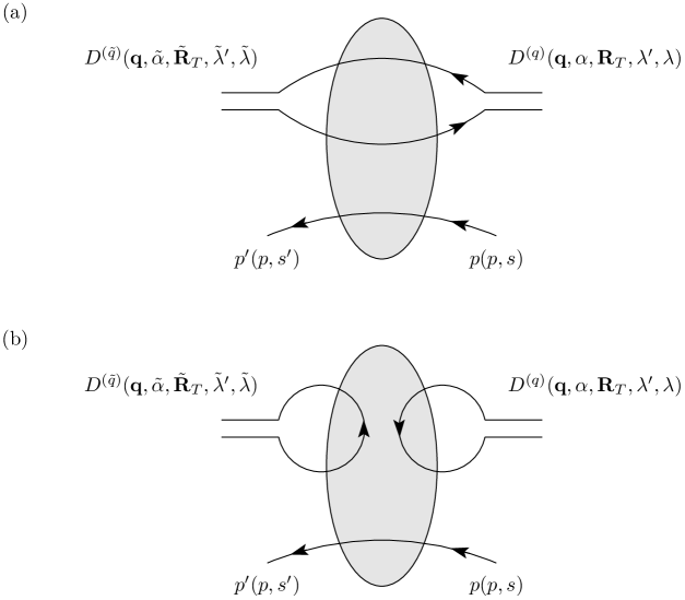
Figure 4: The diagram classes containing the leading contribution to the $T$-matrix element of dipole states in (124) in the high energy limit. The classes (a) and (b) result from the amplitudes ${\cal M}^{(a)}$ and ${\cal M}^{(b)}$ of figure I.LABEL:fig2, respectively.

The shaded blobs indicate again the functional integration over all gluon potentials with a functional measure including the fermion determinant. The discussion of typical diagrams and of the relative size of the diagram classes presented in section I.LABEL:sec:relsize for incoming and outgoing photons holds in exactly the same way here for dipole states. In the following we will generically denote the two contributions to the $T$-matrix for dipole states corresponding to the two diagram classes of figure 4 by ${\cal T}^{(a)}$ and ${\cal T}^{(b)}$, respectively.

The following assumptions will concern the $T$-matrix element of dipole states. Since the dipole picture is usually applied only to the scattering of photons off unpolarised protons we will in fact need to make these assumptions only for the proton spin averaged $T$-matrix element

$$\frac{1}{2}\sum_{s^{\prime},s}\delta_{s^{\prime}s}\langle D^{(\tilde{q})}(\mathbf{q},\tilde{\alpha},\tilde{\mathbf{R}}_{T},\tilde{\lambda}^{\prime},\tilde{\lambda}),p(p,s^{\prime})|{\cal T}|D^{(q)}(\mathbf{q},\alpha,\mathbf{R}_{T},\lambda^{\prime},\lambda),p(p,s)\rangle\,.$$ (125)

We will nevertheless formulate the next two assumptions for the $T$-matrix element before averaging and point out some interesting issues concerning the proton spin in our discussion.

Our third assumption is the following:

• The $T$-matrix element occurring in (124) is diagonal in the quark flavour, in $\alpha$ and $\mathbf{R}_{T}$, and is proportional to the unit matrix in the space of spin orientations of the quark and antiquark in the dipole.

As we will see this assumption is crucial for the dipole picture, but it is far from obvious whether it can be derived on general grounds.

Our assumption (iii) is known to hold for the simplest perturbative diagrams (one of them is shown in figure I.LABEL:fig200), both for the case without or with the resummation of leading logarithms of the energy, see for example [7]. These diagrams also illustrate well the intuitive picture of high energy scattering on which the more general assumption (iii) is based. According to this picture a highly energetic quark or antiquark follows a straight trajectory and does not change its transverse position or its longitudinal momentum by a sizable amount while being scattered in the very forward direction, and similarly one expects its helicity to be conserved. For a discussion of this in a nonperturbative framework see for instance [8, 9]. The interaction would correspondingly be diagonal in flavour, in $\alpha$ and $\mathbf{R}_{T}$, and in the helicity. This picture has been quite successful phenomenologically; it for example forms the basis of all eikonal formulations of high energy scattering. A fully nonperturbative derivation of this picture including an estimate of possible corrections could presumably be done along the lines of [8, 9], but this remains to be worked out.

Let us for instance consider the diagonality of the interaction in the transverse position of the quark. The idea that hadronic states in which the partons have fixed transverse positions become eigenstates of the $T$-matrix in the high energy limit has been put forward already in [10]. In the particular case of the dipole picture one often argues that the typical lifetime of the quark-antiquark pair into which the photon fluctuates is much longer than the typical timescale of the interaction with the proton and that therefore the transverse positions (or other properties) of the quark and antiquark should not change during that interaction. But this argument does not make any reference to the actual dynamics of the interaction and in our opinion would need more rigorous support. While for soft gluon exchanges that argument can be made more concrete [8] the situation remains to be clarified for general interactions. Interestingly, the results found in [11] indicate that the diagonality in $\mathbf{R}_{T}$ is violated already in perturbation theory if one goes beyond the leading logarithmic approximation by taking into account exact gluon kinematics in the framework of $k_{T}$-factorisation [12]. It would be very interesting to study this issue in more detail in the framework of a full calculation in next-to-leading logarithmic approximation. This could lead to a more solid test of the validity of assumption (iii) and hence of the foundation of the dipole picture at least in perturbation theory.

An interesting issue is also the assumption that the helicity of the quark and the antiquark are conserved in the interaction. This helicity conservation has already been found in the perturbative study of various QED processes at high energy, see for example [13, 14, 15]. The results obtained there for the leading terms at high energy can be applied also for gluon exchanges between quarks and hence also hold in QCD. In perturbation theory one finds that there are also contributions involving a helicity flip if one goes to the next-to-leading logarithmic approximation, see for example [16] and references therein. It hence remains an open question to which accuracy the conservation of quark helicities holds in general. An interesting possibility to address this question might be the study of spin-dependent structure functions as we will explain in section 6.3.

As we have pointed out the intuitive picture of high energy scattering described above is reflected in the simplest perturbative diagrams, see for example figure I.LABEL:fig200. But one should remember that those diagrams contribute only to the amplitude ${\cal M}^{(a)}$ and hence to the part ${\cal T}^{(a)}$ of the full $T$-matrix element, see figure 4a. One can easily see that the diagonality in assumption (iii) is plausible only for that part ${\cal T}^{(a)}$. Let us consider the second contribution ${\cal T}^{(b)}$ to the $T$-matrix element (corresponding to the part ${\cal M}^{(b)}$ of the amplitude), see figure 4b. One of the simplest diagrams contributing to ${\cal T}^{(b)}$ is shown in figure I.LABEL:fig200b. The flavours in the two quark loops in this diagram are independent of each other, and the contribution of identical quark flavours in the loops constitutes only the smaller part of the amplitude. Further it appears extremely unlikely that the outgoing quark and antiquark should have a high probability to be produced at the same positions in transverse space and to carry the same longitudinal momentum fractions as the incoming quark and antiquark. Similar considerations can be applied to the full matrix element represented by figure 4b. Hence we can at most expect that the part of the $T$-matrix element corresponding to the amplitude ${\cal M}^{(a)}$ satisfies the assumption (iii).

In the light of this discussion of the simplest perturbative diagrams corresponding to ${\cal T}^{(b)}$ we can say that the above assumption (iii) is likely to exclude most contributions to the scattering amplitude contained in the amplitude ${\cal M}^{(b)}$. However, we cannot make this statement rigorous based on fully nonperturbative considerations. Thus, although it is most probably a consequence of assumption (iii) we formulate it as a separate assumption of the dipole model:

• In the $T$-matrix element in (124) only the contribution ${\cal T}^{(a)}$ is kept while ${\cal T}^{(b)}$ is neglected.

Recall that the amplitude ${\cal M}^{(b)}$ contributes only at higher orders of $\alpha_{s}$ compared to ${\cal M}^{(a)}$, but at low photon virtualities its contribution can well be important.

Finally we need to make the following assumption.

• The proton spin averaged reduced matrix element depends only on $\mathbf{R}^{2}_{T}$ and on $s=(p+q)^{2}$.

This assumption implies in particular that the reduced matrix element is independent of the longitudinal momentum fractions of the quark and antiquark given by $\alpha$. That reflects the usual factorisation of transverse and longitudinal degrees of freedom in high energy reactions. But also for this assumption a general proof is not known.

Note that we have assumed here a dependence of the reduced matrix element on the squared energy $s$ rather than on Bjorken-$x$. We will explain our choice and discuss it in more detail in section 6.4 below.

With the assumptions (iii)-(v) we find for the spin averaged $T$-matrix element at high energy

$$\frac{1}{2}\sum_{s^{\prime},s}\delta_{s^{\prime}s}\langle D^{(\tilde{q})}(\mathbf{q},\tilde{\alpha},\tilde{\mathbf{R}}_{T},\tilde{\lambda}^{\prime},\tilde{\lambda}),p(p,s^{\prime})|{\cal T}|D^{(q)}(\mathbf{q},\alpha,\mathbf{R}_{T},\lambda^{\prime},\lambda),p(p,s)\rangle$$ (126)

$$= {}\delta_{\tilde{q}q}\,\delta_{\tilde{\lambda}^{\prime}\lambda^{\prime}}\,\delta_{\tilde{\lambda}\lambda}\,\delta(\tilde{\alpha}-\alpha)\,\delta^{(2)}(\tilde{\mathbf{R}}_{T}-\mathbf{R}_{T})\,{\cal T}^{(q)}_{\rm red}(\mathbf{R}^{2}_{T},s)\,,$$

where ${\cal T}^{(q)}_{\rm red}$ is the reduced $T$-matrix element and involves only contributions coming from ${\cal T}^{(a)}$. The fact that ${\cal T}^{(q)}_{\rm red}$ is a function of $\mathbf{R}^{2}_{T}$ and $s$ only is an immediate consequence of assumption (v). The more conventional definition of the reduced $T$-matrix element would include all factors depending on the continuous parameters of the $T$-matrix element. Here we have explicitly taken out the two singular factors given by the two delta-functions involving $\alpha$ and $\mathbf{R}_{T}$ in order to have a reduced $T$-matrix element that can as usual be assumed to be a smooth function of its arguments. Alternatively, we could have chosen to approximate the delta-functions involving $\alpha$ and $\mathbf{R}_{T}$ in (126) by strongly peaked but smooth functions and to absorb them into the definition of the reduced matrix element. That would correspond to requiring an approximate diagonality in assumption (iii).

We can now obtain the reduced cross section for the scattering of a dipole state on an unpolarised proton from the reduced $T$-matrix element via the optical theorem,

$$\sigma^{(q)}_{\rm red}(\mathbf{R}^{2}_{T},s)=\frac{1}{s}\,{\rm Im}\,{\cal T}^{(q)}_{\rm red}(\mathbf{R}^{2}_{T},s)\geq 0\,.$$ (127)

Recall that we have assumed that quarks have a mass-shell in assumption (i). Therefore we can now conclude that this reduced cross section is non-negative since it can due to that assumption be related to a physical three-to-three scattering process $q\bar{q}p\to q\bar{q}p$. In this sense we can further below interpret the reduced cross section $\sigma^{(q)}_{\rm red}$ as the cross section for a scattering of a dipole on an unpolarised proton. Note that the reduced cross section can naturally be expected to depend on the quark flavour $q$, for instance via the quark mass $m_{q}$.

Instead of considering the original dipole states $D$ we could also consider the corresponding $T$-matrix element of smeared dipole states $\bar{D}$ as introduced in (5.2). Then we obtain from (126) for large $s$

$$\frac{1}{2}\sum_{s^{\prime},s}\delta_{s^{\prime}s}\langle\bar{D}^{(\tilde{q})}(\mathbf{q},\bar{\alpha},\bar{\mathbf{R}}_{T},\tilde{\lambda}^{\prime},\tilde{\lambda}),p(p,s^{\prime})|{\cal T}|\bar{D}^{(q)}(\mathbf{q},\bar{\alpha},\bar{\mathbf{R}}_{T},\lambda^{\prime},\lambda),p(p,s)\rangle$$ (128)

$$= {}\delta_{\tilde{q}q}\,\delta_{\tilde{\lambda}^{\prime}\lambda^{\prime}}\,\delta_{\tilde{\lambda}\lambda}\,\bar{{\cal T}}^{(q)}_{\rm red}(\bar{\mathbf{R}}^{2}_{T},s)$$

with

$$\bar{{\cal T}}^{(q)}_{\rm red}(\bar{\mathbf{R}}^{2}_{T},s)=\int d^{2}R_{T}\,|f_{T}(\mathbf{R}_{T}-\bar{\mathbf{R}}_{T})|^{2}\,{\cal T}^{(q)}_{\rm red}(\mathbf{R}^{2}_{T},s)\,.$$ (129)

We can interpret $\bar{{\cal T}}^{(q)}_{\rm red}$ as the genuine proton spin averaged $T$-matrix element for smeared dipole states and can assume that it is a smooth function of its arguments. Note that in the matrix element (128) the incoming and outgoing dipole states need to have the same $\bar{\alpha}$ and $\bar{\mathbf{R}}_{T}$ in order to arrive at (129). We can then again invoke the optical theorem to obtain the total cross section for a smeared dipole state, a hadron analogue, scattering on an unpolarised proton for large $s$ as

$$\bar{\sigma}^{(q)}_{\rm red}(\mathbf{\bar{R}}^{2}_{T},s)=\frac{1}{s}\,{\rm Im}\,\bar{{\cal T}}^{(q)}_{\rm red}(\mathbf{\bar{R}}^{2}_{T},s)=\int d^{2}R_{T}\,|f_{T}(\mathbf{R}_{T}-\bar{\mathbf{R}}_{T})|^{2}\,\sigma^{(q)}_{\rm red}(\mathbf{R}^{2}_{T},s)\,.$$ (130)

For a narrow smearing function $f_{T}$ we get $\sigma^{(q)}_{\rm red}(\mathbf{R}^{2}_{T},s)\approx\bar{\sigma}^{(q)}_{\rm red}(\mathbf{R}^{2}_{T},s)$, that is (127) gives a correctly normalised hadron-analogue cross section.

Returning now to the unsmeared dipole states we obtain with (126) from (124)

$$e^{2}\frac{1}{2}\sum_{s^{\prime},s}\delta_{s^{\prime}s}\left.{\cal M}^{\mu\nu}_{s^{\prime}s}(p,p,q)\right|_{\textup{asympt}}\! = {}\!\frac{1}{2\pi m_{p}}\sum_{q}\sum_{\lambda,\lambda^{\prime}}\int^{1}_{0}d\alpha\int d^{2}R_{T}\left(\psi^{(q)\mu}_{\gamma,\lambda\lambda^{\prime}}(\alpha,\mathbf{R}_{T},Q)\right)^{*}$$ (131)

$${}\hskip 28.45274pt{\cal T}^{(q)}_{\rm red}(\mathbf{R}^{2}_{T},s)\,\psi^{(q)\nu}_{\gamma,\lambda\lambda^{\prime}}(\alpha,\mathbf{R}_{T},Q)\,.$$

This gives us for the hadronic tensor of (6.1) at high energy

$$\left.e^{2}W^{\mu\nu}(p,q)\right|_{\textup{asympt}} = \frac{1}{2\pi m_{p}}\sum_{q}\sum_{\lambda,\lambda^{\prime}}\int^{1}_{0}d\alpha\int d^{2}R_{T}\left(\psi^{(q)\mu}_{\gamma,\lambda\lambda^{\prime}}(\alpha,\mathbf{R}_{T},Q)\right)^{*}$$ (132)

$${}\hskip 28.45274pts\,\sigma^{(q)}_{\rm red}(\mathbf{R}^{2}_{T},s)\,\psi^{(q)\nu}_{\gamma,\lambda\lambda^{\prime}}(\alpha,\mathbf{R}_{T},Q)\,.$$

Accordingly, we find with (111) and (112) for $\sigma_{T}$ and $\sigma_{L}$ at high energy

$$\sigma_{T}(s,Q^{2}) = {}\sum_{q}\int d^{2}R_{T}\,w^{(q)}_{T}(R_{T},Q^{2})\,\sigma^{(q)}_{\rm red}(\mathbf{R}^{2}_{T},s)\,,$$ (133)

$$\sigma_{L}(s,Q^{2}) = {}\sum_{q}\int d^{2}R_{T}\,w^{(q)}_{L}(R_{T},Q^{2})\,\sigma^{(q)}_{\rm red}(\mathbf{R}^{2}_{T},s)\,,$$ (134)

where we have defined

$$w^{(q)}_{T}(R_{T},Q^{2}) = {}\sum_{\lambda,\lambda^{\prime}}\int^{1}_{0}d\alpha\,\left|\psi^{(q)\mu}_{\gamma,\lambda\lambda^{\prime}}(\alpha,\mathbf{R}_{T},Q)\,\varepsilon_{+\mu}\right|^{2}$$ (135)

$$= {}\sum_{\lambda,\lambda^{\prime}}\int^{1}_{0}d\alpha\,\left|\psi^{(q)\mu}_{\gamma,\lambda\lambda^{\prime}}(\alpha,\mathbf{R}_{T},Q)\,\varepsilon_{-\mu}\right|^{2}\,,$$

$$w^{(q)}_{L}(R_{T},Q^{2}) = {}\sum_{\lambda,\lambda^{\prime}}\int^{1}_{0}d\alpha\,\left|\psi^{(q)\mu}_{\gamma,\lambda\lambda^{\prime}}(\alpha,\mathbf{R}_{T},Q)\,\varepsilon^{\prime}_{L\mu}\right|^{2}\,.$$ (136)

We recall that in (136) we have to use the polarisation vector $\varepsilon^{\prime}_{L}$ (56) since only then do we get the correct asymptotic expression, as was explained in section 4. Here and in the rest of the paper we only deal with the asymptotic expressions and no longer indicate this by a subscript. Note that $w_{L}^{(q)}$ and $w_{T}^{(q)}$ depend only on $R_{T}$ but not on the orientation of $\mathbf{R}_{T}$ due to (54) and (61).

With (133)-(136) we have finally arrived at the standard formulae for the dipole picture used extensively in the literature, see for example [17]. We have tried to spell out all the assumptions that enter and that should be carefully examined when one wants to draw conclusions, for instance concerning saturation, from a supposed ‘unitarity limit’ for $\sigma_{\rm red}(\mathbf{R}^{2}_{T},s)$. We consider it an important task for the future to test the assumptions and to quantify their accuracy.

Note that in the dipole formulae (133) and (134) $R_{T}$ appears formally as an integration variable. But the interpretation of these formulae as a factorisation into the square of a photon wave function and a cross section for the scattering of a dipole of transverse size $R_{T}$ on a proton is very natural in view of the relation of the latter to the corresponding $T$-matrix element, see (126) and (127). We will therefore simply call $\sigma^{(q)}_{\rm red}$ a dipole cross section in the following. Due to the same relation to a $T$-matrix element involving a particular quark flavour it is also natural that this dipole cross section still depends on that quark flavour $q$.

Next we discuss two issues that we have postponed earlier in this section.

6.3 Proton spin dependence of the dipole cross section

The first point is the dependence on the proton spin. So far we have considered only the scattering of transversely or longitudinally polarised photons on an unpolarised proton, and we have obtained the usual formulae of the dipole picture for the total cross sections of these processes. As a consequence, we needed to make our assumption (iii) only for the proton spin averaged $T$-matrix element (125) rather than for the actual $T$-matrix element which occurs in (124). Nevertheless we have formulated our assumption (iii) for the latter, which amounts to making a stronger assumption. It now seems very interesting to think about possible tests of the dependence of that matrix element on the proton spin. To our knowledge, all models proposed so far for the dipole cross section $\sigma_{\rm red}$ have been used only for calculating scattering processes on unpolarised protons. Some of these models are based on an additional assumption about the proton, namely that it can be considered at high energies as a superposition of colour dipoles described by a suitable weight function for their transverse size and orientation. The scattering process can then be expressed in terms of the cross section of two colour dipoles. In phenomenological applications one hence only needs to make a model for that simpler cross section. For a typical approach along these lines see for example [18]. We emphasise that this assumption goes beyond the dipole picture as we have derived it here, and it is in our opinion far from obvious that the proton can be approximated by a collection of dipoles. It would of course be very interesting to see if that assumption can be justified using the techniques developed in the present work. Let us now for a moment adopt that additional assumption. One expects the dipole-dipole cross section and the corresponding $T$-matrix element to be symmetric under the exchange of the two dipoles at least in the large-$N_{c}$ limit in which a colour dipole can be viewed as a quark-antiquark pair. In assumption (iii) we have assumed that the $T$-matrix element in (124) is proportional to the unit matrix in the space of spin orientations of the quark and antiquark. Accordingly, one would now have to assume that the dipole-dipole $T$-matrix element is also proportional to the unit matrix in the space of spin orientations corresponding to the dipole in the proton. As an immediate consequence one finds that in such a picture the polarised proton structure function $g_{1}$ vanishes. Since this is in contradiction with the experimental findings (for a review see [19]) one might conclude that at least the additional assumption does not hold, but that would be premature. On the contrary, that result would be in agreement with the general finding that the polarised structure function $g_{1}$ is suppressed at high energy with respect to the unpolarised structure function $F_{2}$. It has been established for example in Regge theory that $g_{1}$ is suppressed with respect to $F_{2}$ by a power of the energy [20], and a similar picture emerges also in perturbation theory both in extrapolations of Altarelli-Parisi evolution [21] to small Bjorken-$x$ [22, 23] and in calculations taking into account double-logarithmic contributions beyond Altarelli-Parisi evolution [24, 25]. In many steps of our arguments leading to the dipole picture subleading terms at high energy have been neglected. Thus it is consistent that the leading level result for an observable that starts at a subleading level is zero. Turning this argument around the polarised structure function $g_{1}$ might offer an opportunity to study the structure and the size of subleading terms at high energies. The most important question is of course whether it is possible to find a consistent description of $g_{1}$ (or of any other observable that starts at a subleading level in the expansion in inverse powers of the energy) in the dipole picture. This problem could be studied independently of the additional assumption that the proton can be considered as a superposition of colour dipoles. (Note, however, that that additional assumption is at least consistent with the known results about $g_{1}$.) Further studies along these lines might either show that also subleading terms can be factorised according to the dipole picture, or tell us about a potential breakdown of the dipole picture for subleading terms. In the latter case one could even hope to quantify the size of potential corrections to the dipole picture in general.

6.4 The energy variable of the dipole cross section

The other important issue that we have not yet discussed in detail is the question whether the dipole cross section $\sigma_{\rm red}$ should depend on the squared energy $s$ or on Bjorken-$x$ in addition to the dependence on the dipole size $R_{T}$. Since at high energies $x_{\rm Bj}=Q^{2}/s$ the latter possibility would imply a dependence of the dipole cross section on $Q^{2}$ while such a dependence would be absent if the former possibility were chosen. Phenomenological models for the dipole cross section have been proposed based on both possibilities, and both can lead to a satisfactory description of the available data. Overall, models based on an $x_{\rm Bj}$-dependent dipole cross section appear to be more popular at present. A model with an $s$-dependent dipole cross section has been constructed for instance in [26] while a prominent example for an $x_{\rm Bj}$-dependent dipole cross section is the model of [27]. In our approach we have obtained the dipole cross section from a $T$-matrix element for the scattering of a dipole state on a proton, see (126) and (127). But as we have discussed in section 5.2 the dipole states entering this matrix element are independent of the photon virtuality $Q^{2}$ at high energy as can be seen from the expression for their invariant mass (99), see also the corresponding formulae (105) and (106) for smeared dipole states. The relevant $T$-matrix element thus corresponds to a scattering process in which the initial and final state is independent of $Q^{2}$. According to this observation we have chosen our dipole cross section $\sigma_{\rm red}$ to depend only on $s$ rather than on $x_{\rm Bj}$ in our assumption (v). The main motivation for choosing an $x_{\rm Bj}$-dependence in many phenomenological models comes from studying the simultaneous limit of large $s$ and large $Q^{2}$. In this limit the cross section for photon-proton scattering should agree with the perturbative result obtained in the double-leading logarithmic approximation (DLLA) [28]. As was discussed already in [29] the dipole cross section can in that limit be identified up to factors with the gluon density of the proton. The latter naturally depends on $x_{\rm Bj}$ and $Q^{2}$ and therefore suggests to choose the dependence on $x_{\rm Bj}$ also at lower $Q^{2}$. Can we decide which variable is the correct one for the dipole cross section?

Let us first recall that $\mathbf{R}_{T}$ in (133) and (134) is an integration variable. We can therefore perform a change of variables

$$\mathbf{R}_{T}=\frac{Q_{0}}{Q}\,\mathbf{R}^{\prime}_{T}\,,$$ (137)

where $Q_{0}$ is some fixed momentum scale. Expressing the integrands of (133) and (134) in terms of the new integration variable $\mathbf{R}^{\prime}_{T}$ we obtain formulae similar to the dipole model that contain a factor

$$\hat{\sigma}^{(q)}_{\rm red}(\mathbf{R}^{\prime 2}_{T},Q,x_{\rm Bj})=\sigma^{(q)}_{\rm red}\left(\frac{Q_{0}^{2}}{Q^{2}}\,\mathbf{R}^{\prime 2}_{T},s\right)$$ (138)

which we could define as a reduced cross section that depends on $\mathbf{R}^{\prime 2}_{T}$, $Q$ and $x_{\rm Bj}$ instead of $\mathbf{R}^{2}_{T}$ and $s$. However, in this case $\mathbf{R}^{\prime}_{T}$ is no longer the physical size parameter of the colour dipole. Moreover, the substitution (137) would affect also the other factor in the integrands of (133) and (134) and hence spoil the interpretation of the integrand as a product of an actual dipole-proton cross section with the square of the perturbative photon wave function. We therefore discard the mathematical possibility of changing the integration variable from $\mathbf{R}_{T}$ to $\mathbf{R}^{\prime}_{T}$.

A discussion of $s$ versus $x_{\rm Bj}$ dependence of the dipole cross section was given in chapter 9 of [17] and our remarks below follow the same lines. For large photon virtualities $Q^{2}$ one finds that the integrals in (133) and (134) receive the dominant contribution from small $R_{T}$ due to the shape of the weight factors $w^{(q)}_{T,L}$. For small $R_{T}$ the dipole-proton cross section should become small due to colour transparency, and the typical behaviour to be expected at small $R_{T}$ is $\sigma_{\rm red}(\mathbf{R}_{T}^{2},s)\propto R_{T}^{2}$. Hence a typical ansatz for small $R_{T}$ is

$$\sigma^{(q)}_{\rm red}(R_{T}^{2},s)=R_{T}^{2}\,f\left(\frac{1}{sR_{T}^{2}}\right)\,,$$ (139)

where $f$ is a dimensionless scaling function. Naive scaling arguments suggest this and in QCD we expect (139) to hold up to logarithmic corrections in $R_{T}$. Inserting (139) in (133) and (134) we find that the explicit factor $R_{T}^{2}$ together with the weight functions $w^{(q)}_{T,L}(R_{T},Q^{2})$ and an additional factor $R_{T}$ from the integral measure $d^{2}R_{T}$ leads to a pronounced maximum in the integrands situated at

$$R^{2}_{T\,{\rm max}}=\frac{C^{2}}{Q^{2}+4m_{q}^{2}}$$ (140)

with $C^{2}\simeq 4$, see p. 273 of [17] and figure 9 in section 6.5 below. That is, for large $Q^{2}$ mostly dipoles of size $R_{T\,{\rm max}}$ contribute. We may therefore make the replacement

$$\sigma^{(q)}_{\rm red}(R_{T}^{2},s) \longrightarrow R_{T}^{2}\,f\left(\frac{1}{sR^{2}_{T\,{\rm max}}}\right)\simeq R_{T}^{2}\,f\left(\frac{Q^{2}+4m^{2}_{q}}{sC^{2}}\right)$$ (141)

$$\longrightarrow R_{T}^{2}\,f\left(\frac{x_{\rm Bj}}{C^{2}}\right)\equiv\tilde{\sigma}_{\rm red}^{(q)}(R_{T}^{2},x_{\rm Bj})$$

for $Q^{2}\gg 4m_{q}^{2}$. Hence it is only due to the behaviour of the other factors in the integrands and the explicit factor $R_{T}^{2}$ in (139) that an $s$-dependent $\sigma_{\rm red}$ and an $x_{\rm Bj}$-dependent $\sigma_{\rm red}$ lead to the same result at large $Q^{2}$. It is therefore not possible to establish an $x_{\rm Bj}$-dependence of the dipole cross section in general based on this argument. As we have described above, in our approach an $s$-dependence occurs naturally. We cannot exclude that a different derivation of the dipole picture based on a different set of assumptions is possible in which an $x_{\rm Bj}$-dependence occurs. If one wants to maintain the interpretation of $\sigma_{\rm red}$ as an actual cross section involving a quark-antiquark colour dipole state, however, one would need to define the dipole states in such a way that they depend on $Q^{2}$ in leading order in the expansion in inverse powers of $s$. This would in particular exclude the natural definition (95) which we have used.

In this context we should add a further remark. It would of course be interesting to establish the relation of our derivation of the dipole picture with the perturbative picture of the DLLA step by step. But there is a potential problem. In the present paper we study the limit

$$s\to\infty\,,\>\>\>\>\>Q^{2}\,\,{\rm fixed}\,,$$ (142)

whereas in the DLLA one takes

$$s\to\infty\,,\>\>\>\>\>Q^{2}\to\infty\,,\>\>\>\>\>\frac{Q^{2}}{s}\,\,{\rm fixed}\,.$$ (143)

It is not at all clear and not necessary that first taking the limit (142) and then letting $Q^{2}$ become large will lead to the same result as taking the limit (143). It remains to be seen whether this makes the comparison of our derivation with the perturbative approach intrinsically difficult.

6.5 Density for the photon wave function in leading order

In the dipole picture the photon-proton cross section is obtained as the convolution of the square of the photon wave function with the dipole cross section. The latter cannot be calculated from first principles at present and needs to be described by models in phenomenological applications of the dipole picture. The photon wave function, on the other hand, is known explicitly in perturbation theory. We therefore find it useful to discuss here some known aspects of the photon wave function and to illustrate some of its properties. In the next section we will then derive some phenomenological consequences of the dipole picture which will be based only on the properties of the perturbative photon wave function but will not depend on any particular model assumptions about the dipole cross section.

In the following we consider the densities

$$v^{(q)}_{T}(\alpha,R_{T},Q^{2}) = \sum_{\lambda,\lambda^{\prime}}\left|\psi_{\gamma,\lambda\lambda^{\prime}}^{(q)+}(\alpha,\mathbf{R}_{T},Q)\right|^{2}$$

$$= {}\frac{N_{c}}{2\pi^{2}}\,\alpha_{\rm em}Q_{q}^{2}\left\{\left[\alpha^{2}+(1-\alpha)^{2}\right]\epsilon_{q}^{2}[K_{1}(\epsilon_{q}R_{T})]^{2}+m_{q}^{2}[K_{0}(\epsilon_{q}R_{T})]^{2}\right\}$$

and

$$v^{(q)}_{L}(\alpha,R_{T},Q^{2}) = \sum_{\lambda,\lambda^{\prime}}\left|\psi_{\gamma,\lambda\lambda^{\prime}}^{(q)L}(\alpha,\mathbf{R}_{T},Q)\right|^{2}$$ (145)

$$= {}\frac{2N_{c}}{\pi^{2}}\,\alpha_{\rm em}Q_{q}^{2}Q^{2}[\alpha(1-\alpha)]^{2}[K_{0}(\epsilon_{q}R_{T})]^{2}$$

for transversely and longitudinally polarised photons as obtained from the respective photon wave functions in leading order, see (54), (61) and (50). Upon integration over the longitudinal momentum fraction $\alpha$ these densities give the functions $w_{T}$ and $w_{L}$ in (135) and (136) that occur in the dipole formulae (133) and (134),

$$w^{(q)}_{T/L}(R_{T},Q^{2})=\int_{0}^{1}d\alpha\,v^{(q)}_{T/L}(\alpha,R_{T},Q^{2})\,.$$ (146)

For our numerical results we assume the light quarks ($q=u,d,s$) to be massless while for the heavy quark masses we use $m_{c}=1.3\,\mbox{GeV}$ and $m_{b}=4.6\,\mbox{GeV}$.

We start with transversely polarised photons. Figure 5 shows the dependence of the density $v^{(q)}_{T}/(\alpha_{\rm em}Q_{q}^{2})$ on the longitudinal momentum fraction $\alpha$ for fixed $R_{T}\!=\!1\,\mbox{GeV}^{-1}$ and for three different values of the photon virtuality $Q^{2}=1,10,100\,\mbox{GeV}^{2}$. The left panel is for massless ($u,d,s$) quarks while the right panel is for $c$- and $b$-quarks.

Figure 5: Dependence of the density $\frac{1}{\alpha_{\rm em}Q_{q}^{2}}\,v^{(q)}_{T}(\alpha,R_{T},Q^{2})$ of transversely polarised photons (see (6.5)) on $\alpha$ for $R_{T}\!=\!1\,\mbox{GeV}^{-1}$ and for three different values $Q^{2}=1,10,100\,\mbox{GeV}^{2}$, plotted in units of $\mbox{GeV}^{2}$; on the left for massless ($q=u,d,s$) quarks, on the right for $c$-quarks (upper lines) and $b$-quarks (lower lines).

Note that for transversely polarised photons there is a nonvanishing contribution from the end points $\alpha=0$ and $\alpha=1$ even for very large photon virtualities $Q^{2}$. As can be seen also from (6.5) the value of $v^{(q)}_{T}$ at these end points depends on the mass of the quark flavour under consideration. The density has a minimum at $\alpha=1/2$ for all values of $Q^{2}$ and the relative size of the density at this minimum compared to the end points shrinks with increasing $Q^{2}$. That means that a symmetric distribution of the longitudinal momentum of the photon between the quark and antiquark is the least likely configuration, and this effect becomes more pronounced for larger $Q^{2}$. The size of the density decreases rapidly with increasing $Q^{2}$ for all $\alpha$ with the exception of the end points. Figure 6 shows the dependence of $v^{(q)}_{T}/(\alpha_{\rm em}Q_{q}^{2})$ on $\alpha$ for fixed photon virtuality $Q^{2}\!=\!10\,\mbox{GeV}^{2}$ and for three different values of the dipole size $R_{T}=0.1,1,5\,\mbox{GeV}^{-1}$, again for massless quarks on the left and for massive quarks on the right.

Figure 6: Dependence of the density $\frac{1}{\alpha_{\rm em}Q_{q}^{2}}\,v^{(q)}_{T}(\alpha,R_{T},Q^{2})$ of transversely polarised photons (see (6.5)) on $\alpha$ for $Q^{2}\!=\!10\,\mbox{GeV}^{2}$ and for three different values $R_{T}=0.1,1,5\,\mbox{GeV}^{-1}$, plotted in units of $\mbox{GeV}^{2}$; on the left for massless ($q=u,d,s$) quarks, on the right for $c$-quarks (upper lines for each line type) and $b$-quarks (lower lines for each line type).

While for $R_{T}=0.1\,\mbox{GeV}^{-1}$ the densities for $c$- and $b$-quarks cannot be distinguished when plotted on a logarithmic scale like in figure 6 their sizes become very different for larger $R_{T}$. Already for $R_{T}=5\,\mbox{GeV}^{-1}$ the density for the $b$-quark is so small that it is far below the range shown in the figure. For all quark flavours the dependence of the density on $\alpha$ changes with $R_{T}$ in a similar way as it changes with $Q$, in particular it decreases rapidly with increasing $R_{T}$ for all momentum fractions $\alpha$. For massless quarks this similarity can be understood immediately based on dimensional arguments. Namely, for massless quarks the dependence of the density on $Q^{2}$ is related to the dependence on $R_{T}$ because the dimensionless quantity $R_{T}^{2}v^{(q)}_{T}$ can depend only on the product $QR_{T}$ by dimensions. However, we have plotted the dimensionful density $v_{T}$ in our figures and hence the values of the density at the end points $\alpha=0$ and $\alpha=1$ are different for different values of $R_{T}$.

Next we turn to longitudinally polarised photons. In figure 7 we show the dependence of the density $v^{(q)}_{L}/(\alpha_{\rm em}Q_{q}^{2})$ on the longitudinal momentum fraction $\alpha$ for fixed $R_{T}\!=\!1\,\mbox{GeV}^{-1}$ and for three different values of the photon virtuality $Q^{2}=1,10,100\,\mbox{GeV}^{2}$. The left panel is again for massless ($u,d,s$) quarks while the right panel is for $c$- and $b$-quarks.

Figure 7: Dependence of the density $\frac{1}{\alpha_{\rm em}Q_{q}^{2}}\,v^{(q)}_{L}(\alpha,R_{T},Q^{2})$ of longitudinally polarised photons (see (145)) on $\alpha$ for $R_{T}\!=\!1\,\mbox{GeV}^{-1}$ and for three different values $Q^{2}=1,10,100\,\mbox{GeV}^{2}$, plotted in units of $\mbox{GeV}^{2}$; on the left for massless ($q=u,d,s$) quarks, on the right for $c$-quarks (upper lines) and $b$-quarks (lower lines).

In the case of longitudinally polarised photons the density vanishes at the end points $\alpha=0$ and $\alpha=1$ for all photon virtualities $Q^{2}$ and for all quark flavours. For small photon virtualities the density has a maximum at $\alpha=1/2$. For larger $Q^{2}$ the symmetric distribution of the longitudinal momentum of the photon between the quark and the antiquark becomes less likely and there appears a local minimum in the density at $\alpha=1/2$. At the same time two maxima of the density develop close to the end points $\alpha=0$ and $\alpha=1$. For massless quarks the overall size of the density decreases rapidly with increasing $Q^{2}$, except for small regions close to the end points where the maxima appear at larger $Q^{2}$. For massive quarks that overall decrease with $Q^{2}$ sets in only for $Q^{2}>m_{q}^{2}$. Figure 8 shows the dependence of the density on $\alpha$ for fixed photon virtuality $Q^{2}\!=\!10\,\mbox{GeV}^{2}$ and for three different values $R_{T}=0.1,1,5\,\mbox{GeV}^{-1}$, again for massless quarks on the left and for massive quarks on the right.

Figure 8: Dependence of the density $\frac{1}{\alpha_{\rm em}Q_{q}^{2}}\,v^{(q)}_{L}(\alpha,R_{T},Q^{2})$ of longitudinally polarised photons (see (145)) on $\alpha$ for $Q^{2}\!=\!10\,\mbox{GeV}^{2}$ and for three different values $R_{T}=0.1,1,5\,\mbox{GeV}^{-1}$, plotted in units of $\mbox{GeV}^{2}$; on the left for massless ($q=u,d,s$) quarks, on the right for $c$-quarks (upper lines for each line type) and $b$-quarks (lower lines for each line type).

The size of the density decreases with increasing $R_{T}$, and for $R_{T}=5\,\mbox{GeV}^{-1}$ the density for $b$-quarks is already so small that it is far below the range shown in the figure. For massless quarks the dependence of the density on $R_{T}$ can again be deduced from the dependence on $Q^{2}$ via the dimensionless quantity $R_{T}^{2}v^{(q)}_{L}$ which depends only on $QR_{T}$. For large $R_{T}$ the dependence of the density for massive quarks on $R_{T}$ follows a pattern similar to that of massless quarks.

Finally, we consider the dimensionless quantity $QR_{T}^{3}w^{(q)}_{T,L}$ for transversely and longitudinally polarised photons which occurred in our discussion of the energy variable of the dipole cross section in section 6.4. There we pointed out that the densities $w^{(q)}_{T,L}$ occur in the dipole formulae (133) and (134) together with a factor $R_{T}$ from the integral measure and another factor of $R_{T}^{2}$ coming from the dipole cross section at small $R_{T}$, see (139). Multiplying by $Q$ leads us to the dimensionless quantity $QR_{T}^{3}w^{(q)}_{T,L}$. We recall that $w^{(q)}_{T,L}$ is obtained from $v^{(q)}_{T,L}$ in (6.5) and (145) by integrating over $\alpha$, see (146). Figure 9 shows the dependence of $QR_{T}^{3}w^{(q)}_{T,L}$ on $R_{T}$ for massless quarks ($q=u,d,s$) and for three different photon virtualities $Q^{2}=1,10,100\,\mbox{GeV}^{2}$.

Figure 9: Dependence of the dimensionless quantity $QR_{T}^{3}w^{(q)}_{T,L}$ on $R_{T}$ for massless ($q=u,d,s$) quarks for three different values $Q^{2}=1,10,100\,\mbox{GeV}^{2}$; on the left for transversely polarised photons, on the right for longitudinally polarised photons.

The left panel is for transversely polarised photons and the right panel for longitudinally polarised photons. The figure shows that there are indeed pronounced maxima, and their position $R_{T{\rm max}}$ scales with $1/Q$, see also (140). For transversely polarised photons the maxima turn out to be wider than for longitudinally polarised photons. Since for massless quarks the dimensionless $QR_{T}^{3}w^{(q)}_{T,L}$ can depend only on $QR_{T}$ the value of this quantity at the maximum is the same for all $Q^{2}$ here.

7 A bound on $R=\sigma_{L}/\sigma_{T}$ from the dipole picture 

In the previous section we have obtained the dipole picture of high energy scattering based on a number of assumptions. It is obviously important to test these assumptions and to find the range of kinematical parameters in which they hold, or in other words, the range in which the dipole picture can be applied.

In the dipole picture the cross section for photon-proton scattering is written as a convolution of the square of the perturbative photon wave function with the dipole-proton cross section, see (133) and (134). The former can be determined explicitly in perturbation theory (see section 4) while the latter cannot be calculated from first principles at present. Especially in the interesting region of intermediate and low photon virtualities one therefore has to retreat to models for the dipole cross section which can then be tested against the available data. Although the required agreement with the data places constraints on the possible models for the dipole cross section there is still considerable freedom in these models. Based on such models it is therefore difficult to test the assumptions on which the dipole picture is based and to explore their potential limits. It would hence appear favourable to find observables which can be used to test the assumptions of the dipole picture in a way which does not depend on any particular model for the dipole cross section.

In the present section we want to study such an observable, namely the ratio $R$ of the cross sections for longitudinally and transversely polarised photons,

$$R(s,Q^{2})=\frac{\sigma_{L}(s,Q^{2})}{\sigma_{T}(s,Q^{2})}\,.$$ (147)

In the following we will derive a bound on $R$ from the dipole picture which will involve only the properties of the perturbative wave functions of longitudinally and transversely polarised photons.

First we recall that the quantities $w^{(q)}_{T}$ and $w^{(q)}_{L}$ in (135) and (136) are positive since they are obtained as integrals over the squared modulus of the perturbative photon wave function. Further we recall that the dipole cross section is non-negative according to our assumptions made in section 6.2, see (127). We then start from the obvious relation

$$\frac{w^{(q)}_{L}(R_{T},Q^{2})}{w^{(q)}_{T}(R_{T},Q^{2})}\,\leq\,\max_{q,R_{T}}\,\frac{w^{(q)}_{L}(R_{T},Q^{2})}{w^{(q)}_{T}(R_{T},Q^{2})}\,,$$ (148)

where the maximum is taken over all dipole sizes $R_{T}$ and over all quark flavours $q$. We then multiply both sides of this relation by the positive quantity $w^{(q)}_{T}(R_{T},Q^{2})$ and by the dipole cross section $\sigma^{(q)}_{\rm red}(R^{2}_{T},s)$ which is non-negative. Next we integrate over $\mathbf{R}_{T}$ and sum over all quark flavours which gives with the dipole formulae (133) and (134)

$$\sigma_{L}(s,Q^{2})\,\leq\,\sigma_{T}(s,Q^{2})\,\max_{q,R_{T}}\,\frac{w^{(q)}_{L}(R_{T},Q^{2})}{w^{(q)}_{T}(R_{T},Q^{2})}\,.$$ (149)

An analogous relation is readily obtained for the minimum of $w^{(q)}_{L}/w^{(q)}_{T}$, such that we have

$$\min_{q,R_{T}}\,\frac{w^{(q)}_{L}(R_{T},Q^{2})}{w^{(q)}_{T}(R_{T},Q^{2})}\,\leq\,R(s,Q^{2})\,\leq\,\max_{q,R_{T}}\,\frac{w^{(q)}_{L}(R_{T},Q^{2})}{w^{(q)}_{T}(R_{T},Q^{2})}\,.$$ (150)

With this relation we have obtained an upper and a lower bound on the ratio $R(s,Q^{2})$ which should be respected for all $s$ and $Q^{2}$ for which the dipole picture is valid or – phrased differently – for which the assumptions and approximations (i)-(v) hold which we have discussed in section 6.2. Note that the bounds (150) depend only on the photon virtuality $Q^{2}$ but do not depend on $s$. This is of course expected since the bounds involve only the photon wave function but not the dipole cross section $\sigma_{\rm red}(R_{T}^{2},s)$, and only the latter contains the energy dependence of $\sigma_{T}$ and $\sigma_{L}$ according to the dipole formulae (133) and (134).

Similarly, we can obtain bounds for the ratio of the cross sections for the production of a heavy quark flavour, $q=c$ or $q=b$, in deep inelastic scattering,

$$\min_{R_{T}}\,\frac{w^{(q)}_{L}(R_{T},Q^{2})}{w^{(q)}_{T}(R_{T},Q^{2})}\,\leq\,R_{q}(s,Q^{2})=\frac{\sigma^{(q)}_{L}(s,Q^{2})}{\sigma^{(q)}_{T}(s,Q^{2})}\,\leq\,\max_{R_{T}}\,\frac{w^{(q)}_{L}(R_{T},Q^{2})}{w^{(q)}_{T}(R_{T},Q^{2})}\,.$$ (151)

Let us now determine the numerical values of the bounds derived here. In figure 10 we show the ratio $w_{L}^{(q)}(R_{T},Q^{2})/w_{T}^{(q)}(R_{T},Q^{2})$ for massless ($q=u,d,s$) quarks as a function of $R_{T}$ for a particular value $Q^{2}\!=\!10\,\mbox{GeV}^{2}$.

Figure 10: The ratio $w_{L}^{(q)}(R_{T},Q^{2})/w_{T}^{(q)}(R_{T},Q^{2})$ as a function of $R_{T}$ for $Q^{2}\!=\!10\,\mbox{GeV}^{2}$ for massless ($q=u,d,s$) quarks.

This ratio has a maximum at which its value is $0.37248$, and asymptotically it approaches zero. Since $w^{(q)}_{L}/w^{(q)}_{T}$ is a dimensionless quantity it can for massless quarks depend only on $QR_{T}$ such that also for different photon virtualities $Q^{2}$ we find a maximum with the same value. For massive quarks ($q=c,b$) the ratio $w^{(q)}_{L}/w^{(q)}_{T}$ as a function of $R_{T}$ also exhibits a maximum with a value which now depends on $Q^{2}$, but for all $Q^{2}$ we find that this value is smaller than for massless quarks.

We can therefore conclude that the upper bound on $R$ in (150) gives

$$R(s,Q^{2})\leq 0.37248\,,$$ (152)

while the lower bound on $R$ in (150) reduces to the trivial statement that $R$ is non-negative. Also the lower bound on the ratios $R_{c}$ and $R_{b}$ in (151) is trivial. The upper bounds on $R_{c}$ and $R_{b}$ resulting from (151), on the other hand, are nontrivial and depend on $Q^{2}$. This dependence is shown in figure 11 together with the upper bound (152) on $R$.

Figure 11: The upper bound on $R=\sigma_{L}/\sigma_{T}$ resulting from the dipole model as a function of $Q^{2}$. The solid line is for massless ($u$, $d$, $s$) quarks and constitutes the bound (150). The lower lines are upper bounds on $R_{c}=\sigma^{(c)}_{L}/\sigma^{(c)}_{T}$ and $R_{b}=\sigma^{(b)}_{L}/\sigma^{(b)}_{T}$, respectively, see (151).

In many practical applications of the dipole picture one chooses to introduce phenomenological masses for the light ($q=u,d,s$) quarks. In [27] for example a light quark mass of $m_{q}=140\,\mbox{MeV}$ is chosen, and this mass is implemented in the perturbative photon wave function. Such a modified photon wave function results in a corresponding modification of the bound on $R$ which then becomes $Q^{2}$-dependent. For $m_{q}=140\,\mbox{MeV}$ this bound is shown on a linear scale in figure 14 below. With the logarithmic $Q^{2}$-scale in figure 11 it would correspond to a curve of the same shape as the bound on $R_{c}$ or $R_{b}$ but shifted to the left such that its value at $Q^{2}=1\,\mbox{GeV}^{2}$ would be $0.318$.

A popular extension of the dipole picture as we have discussed it so far is to diffractive deep inelastic scattering. In this extension one usually writes for the diffractive photon-proton cross section [31]

$$\left.\frac{d\sigma^{\rm diff}_{T/L}}{dt}\right|_{t=0}\!\!(s,Q^{2})=\frac{1}{16\pi}\sum_{q}\int d^{2}R_{T}\,w^{(q)}_{T/L}(R_{T},Q^{2})\,\left(\sigma^{(q)}_{\rm red}(\mathbf{R}^{2}_{T},s)\right)^{2}\,,$$ (153)

where the dipole cross section $\sigma_{\rm red}$ is the same as in the usual dipole picture. The dipole formula for diffractive scattering (153) therefore relates diffractive to inclusive photon-proton scattering. Accepting (153) as a valid description of the diffractive cross section one finds that exactly the same bounds as obtained above apply also to diffractive photon-proton scattering, both for the total diffractive cross section and for diffractive production of heavy quarks. In particular, we have

$$\frac{\left.\frac{\sigma^{\rm diff}_{L}}{dt}\right|_{t=0}\!\!(s,Q^{2})}{\left.\frac{\sigma^{\rm diff}_{T}}{dt}\right|_{t=0}\!\!(s,Q^{2})}\leq 0.37248\,.$$ (154)

We emphasise, however, that the extension of the dipole picture to diffractive scattering (153) goes beyond what we have discussed so far in the present work. It is in particular not clear and in fact not necessary that the dipole formula (153) for diffractive scattering follows from the same assumptions (i)-(v) which we have used to obtain the dipole picture for inclusive deep inelastic scattering. It is an open question whether it is possible to establish the dipole picture of diffractive photon-proton scattering based on the techniques presented here.

The dipole picture has been applied also to a number of exclusive reactions, a typical example is diffractive vector meson production. Here the wave function of the outgoing photon is replaced by the wave function of the produced vector meson, and the latter usually involves some model assumptions. We should point out that our bounds on $R$ cannot be applied directly to such processes. This is because our derivation of the bounds relies on the positivity of both factors under the integrals in the dipole formulae (133) and (134). In particular, it relies on the positivity of the square of the photon wave function which occurs due to the incoming and the outgoing photon. In other reactions that factor is changed and positivity is in general not guaranteed.

We now return to inclusive deep inelastic photon-proton scattering and discuss the experimental data on $R$. The presently available data on $R$ at high energies have been obtained by the NMC [32], CCFR [33], E143 [34], EMC [35] and CDHSW [36] collaborations. The scattering processes used to extract $R$ include not only $e^{\pm}p$ scattering but also a variety of other scattering processes including muon and neutrino scattering on nuclear targets. In some of these processes one might in general expect additional caveats concerning the applicability of the dipole picture. For lack of further experimental data we nevertheless include the corresponding data points here. At high energies $R$ is expected to be independent of the target, as is also confirmed by the data within the experimental errors. For further details we refer the reader to the experimental publications.

We want to consider only data points at sufficiently high energy which we choose to be data with $x_{\rm Bj}<0.05$. Figure 12 shows all available data in this energy region together with the bound (152) resulting from the dipole picture.

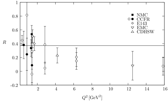
Figure 12: Comparison of experimental data for $R=\sigma_{L}/\sigma_{T}$ in the region $x_{\rm Bj}<0.05$ with the bound (152) resulting from the dipole picture. Full points correspond to data with $x_{\rm Bj}<0.01$, open points are data with $0.01<x_{\rm Bj}\leq 0.05$.

The few data points available at $x_{\rm Bj}<0.01$ are shown as full points while those with $0.01\leq x_{\rm Bj}<0.05$ are shown as open points. The data have rather large errors, but by and large we can say that they respect the bound resulting from the dipole picture. For $Q^{2}$ below $2\,\mbox{GeV}^{2}$, however, there appears to be the tendency that the data come close to the bound. Note the interesting fact that data very close to the bound (152) could be accommodated in the dipole picture only if the dipole cross section $\sigma_{\rm red}$ were strongly peaked in $R_{T}$ around the maximum of $w^{(q)}_{L}/w^{(q)}_{T}$ – which would appear to be very unlikely in reality. Hence already data close to the bound could be interpreted as an indication of the breakdown of the dipole picture. The errors of presently available data are far too large to draw any firm conclusion about the assumptions underlying the dipole picture here, but we might take them as an indication for the values of $Q^{2}$ below which we should be careful in interpreting scattering processes in terms of the dipole picture only.

Unfortunately, no direct measurements of $F_{L}$ and $R$ have been performed at HERA so far. A discussion of the available indirect determinations of $F_{L}$ in view of our bound will be given elsewhere. Direct measurements of $F_{L}$ at HERA are planned and will hopefully lead to a better determination of $R$, allowing for a stringent test of the validity of the dipole picture at low $Q^{2}$. Also a potential future upgrade of RHIC to an electron-ion collider eRHIC would offer the possibility to obtain a clear picture of $R$ at high energies and low $Q^{2}$, and thus to establish a conclusive test of the dipole picture in this region.

Let us finally see which behaviour of $R(s,Q^{2})$ is predicted in the framework of a typical model for the dipole cross section $\sigma_{\rm red}$. As a prominent example we choose the Golec-Biernat-Wüsthoff model [27]. In that model the dipole cross section is assumed to be a function of $R_{T}^{2}$, $x_{\rm Bj}$ and $Q^{2}$ and not only of $R_{T}^{2}$ and $s$. This might pose a problem in the context of our discussion in section 6.4 but for the purpose of illustrating the behaviour of $R$ in a typical dipole model we can disregard this issue. We should point out in this context that our bound (152) is completely independent of the variables on which the dipole cross section depends. In the Golec-Biernat-Wüsthoff model the dipole cross section $\sigma_{\rm red}$ is given by

$$\sigma^{(q)}_{\rm GBW}=\sigma_{0}\left[1-\exp\left(-\frac{R_{T}^{2}}{4R_{0}^{2}}\right)\right]$$ (155)

with

$$R_{0}^{2}(\tilde{x})=\left(\frac{\tilde{x}}{x_{0}}\right)^{\lambda}\,\mbox{GeV}^{-2}\,,$$ (156)

where the three parameters of the model are chosen to be $\sigma_{0}=23\,\mbox{mb}$, $\lambda=0.29$, $x_{0}=3\cdot 10^{-4}$. The variable $\tilde{x}$ in (156) is obtained from $x_{\rm Bj}$ via

$$\tilde{x}=x_{\rm Bj}\left(1+\frac{4m_{q}^{2}}{Q^{2}}\right)\,,$$ (157)

due to which the dependence of $\sigma_{\rm GBW}$ on the quark flavour and on $Q^{2}$ enters. We use again $m_{c}=1.3\,\mbox{GeV}$ for the charm quark mass. In order to study the photoproduction limit $Q^{2}\to 0$ a phenomenological mass of $m^{\rm GBW}_{q}=140\,\mbox{MeV}$ is chosen for the light quarks ($q=u,d,s$) which serves as a regulator for logarithmic divergences that would otherwise occur in this limit. In the Golec-Biernat-Wüsthoff model [27] that phenomenological light quark mass is implemented not only in the dipole cross section via (157) but also in the photon wave function. Note, however, that after inclusion of the effects of DGLAP evolution a better fit to the data is obtained with a vanishing light quark mass [37].

In order to compare with our bound (152) we first insert the dipole cross section $\sigma_{\rm GBW}$ (155)-(157) with the light quark mass $m^{\rm GBW}_{q}=140\,\mbox{MeV}$ into the dipole formulae (133) and (134) but keep the light quarks massless in the photon wave functions. The resulting behaviour of $R$ as a function of $Q^{2}$ is shown in figure 13 for four different values of $x_{\rm Bj}$, $x_{\rm Bj}=0.05,0.01,10^{-3},10^{-4}$, together with the bound (152).

Figure 13: The ratio $R=\sigma_{L}/\sigma_{T}$ as obtained from the Golec-Biernat-Wüsthoff model as given by (155)-(157) but with vanishing light quark mass in the photon wave function. The solid lines are for four different values $x_{\rm Bj}=0.05,0.01,10^{-3},10^{-4}$ from bottom to top at large $Q^{2}$. The dashed line is the bound (152) derived from the dipole picture.

The prediction for $R$ depends only weakly on $x_{\rm Bj}$ and stays significantly below the bound.

Next we consider the original Golec-Biernat-Wüsthoff model, that is we implement the phenomenological light quark mass $m^{\rm GBW}_{q}=140\,\mbox{MeV}$ not only in the dipole cross section but also in the photon wave function. The resulting $Q^{2}$-dependence of $R$ for $x_{\rm Bj}=0.01$ is shown as the solid line in figure 14.

Figure 14: The ratio $R=\sigma_{L}/\sigma_{T}$ as obtained from the Golec-Biernat-Wüsthoff model in comparison with the bound on $R$. The solid line results from the model (155)-(157) for $x_{\rm Bj}=0.01$ with the light quark mass $140\,\mbox{MeV}$ in the dipole cross section and in the photon wave function, the dashed line is obtained if that light quark mass is used only in the dipole cross section. The dotted line is the bound (152) and the dot-dashed line is the modified bound as obtained for a light quark mass of $140\,\mbox{MeV}$.

The dashed line in that figure is the one which we obtained before in figure 13 by using the light quark mass $m^{\rm GBW}_{q}$ only in the dipole cross section. At low $Q^{2}$ the phenomenological quark mass leads to a significant suppression of $R$ while for $Q^{2}>3\,\mbox{GeV}^{2}$ the light quark mass in the photon wave function does not have a significant effect. A comparison with figure 12 shows that, given the large errors of the data, both curves are in agreement with the measurements of $R$. The dot-dashed line in figure 14 is the bound obtained from a photon wave function with a light quark mass of $140\,\mbox{MeV}$ as we discussed it already earlier in this section. For photon virtualities $Q^{2}$ below about $2\,\mbox{GeV}^{2}$ the bound is significantly below the original bound (152) which was obtained for massless light quarks and which is shown in the figure as the dotted line.

More precise data on $R$ might in the future serve as an additional test of the quality of various models for the dipole cross section. It would therefore be interesting to study in more detail the behaviour of $R$ also in other models for the dipole cross section. An interesting aspect of such studies could be in particular the choice of a suitable phenomenological light quark mass which is required for the photoproduction limit or is motivated by the expected breakdown of the perturbative description of the photon wave function at large dipole sizes. For a consistent description one should clearly use the same light quark mass in the photon wave function and in the model for the dipole cross section. Since the bound on $R$ depends on the mass of the light quarks in the photon wave function especially at low $Q^{2}$ it would even be possible to use more precise data on $R$ in that region to obtain bounds on possible choices of a phenomenological mass for light quarks in the photon wave function and hence also in models for the dipole cross section.

8 Conclusions and outlook

In this paper and in the companion paper I we have studied how the dipole picture of high energy scattering can be derived in the framework of a genuinely nonperturbative formulation of photon-nucleon scattering. We have analysed in detail the Compton amplitude for real and virtual photons and have isolated the contributions to it which are leading at high energies. We have taken into account properly the renormalisation of these contributions and have studied their gauge invariance emphasising in particular its relevance for the definition of the perturbative photon wave function. We have then identified the approximations and assumptions which are necessary to arrive at the usual dipole picture.

At high energies we obtain indeed the dipole picture, but also find two important additional contributions. One of them corresponds to rescattering effects of the quark and antiquark forming the colour dipole. The other additional contribution corresponds to diagrams in which the incoming photon and the outgoing photon do not couple to the same quark loop. Both of these terms are of higher order in the coupling constant $\alpha_{s}$ but are not suppressed by powers of the energy. In lowest order in perturbation theory these two additional terms do not contribute, and one is left with only the usual dipole picture. At low photon virtualities on the other hand we expect that both additional contributions can have sizable effects. We expect for example that the rescattering term will play an important role in the transition to low photon virtualities for which vector meson dominance applies. The rescattering term should in fact generate the relevant diagrams for the formation of quark-antiquark bound states. It would therefore be very interesting to see whether our results can be used to obtain a better picture of the transition from a perturbative photon wave function at high virtualities to vector meson dominance at low virtualities.

A crucial question in all phenomenological applications of the dipole picture concerns the range of its applicability, or in other words the kinematical region in which the approximations and assumptions leading to the dipole model hold. We have derived a bound on the ratio $R$ of the cross sections for the scattering of longitudinally and transversely polarised photons off hadrons which is relevant in this context. The bound is obtained only from the perturbative photon wave function and is independent of any particular model for the dipole-proton cross section. Therefore it allows for a model independent test of the dipole picture. Unfortunately the presently available data are not precise enough to restrict the range of applicability of the dipole picture. However, the data appear to come close to the bound below photon virtualities of about $2\,\mbox{GeV}^{2}$, suggesting that at least in that region one should be careful in interpreting high energy scattering data in terms of the dipole picture only. In [30] we have presented further bounds on ratios of nucleon structure functions $F_{2}$ taken at the same energy $\sqrt{s}$ but at different photon virtualities $Q^{2}$ resulting from the dipole picture. They are suitable for further constraining the range of applicability of the dipole picture.

The dipole picture is often discussed in the context of the space-time picture of high energy photon-hadron scattering in the target rest frame. Here the photon splits into a long-lived quark-antiquark pair which then interacts with the hadron. Our study confirms this space-time picture and supplements it with the renormalisation of the photon-quark-antiquark vertex. The space-time picture is closely related to the notion of the light-cone wave function of the photon, suggesting a Hamiltonian picture of the evolution of the photon wave function and of the scattering process. We emphasise that we have obtained the dipole picture in a purely Lagrangian approach here. This allowed us in particular to implement the renormalisation procedure in a simple and transparent way. In a Hamiltonian approach a natural extension of the dipole picture is to include higher Fock states in the photon wave function. In a first step one would include for example the quark-antiquark-gluon component of that wave function. As we have already pointed out in I we do not expect to see such higher Fock states in the decompositions of the Compton amplitude which we have performed. We emphasise that they are not missing in our approach. Gluon emissions from the quark and antiquark are in our approach contained both in the rescattering term and in the dipole-nucleon cross section. It would be interesting to study in detail whether and how a consistent separation of such contributions into parts belonging to the photon wave function and to the dipole-nucleon scattering amplitude can be done. Naturally one would expect that this separation would require to introduce a factorisation scale. We recall that in the usual dipole picture the factorisation of the cross section into the square of the photon wave function and a dipole-proton cross section does not involve such a factorisation scale.

We consider it an important task for future work to establish a closer relation of our approach with perturbation theory. It should be possible to follow our derivation of the dipole picture step by step in a perturbative setting. We have for example checked our results concerning the different choices for the polarisation vector for longitudinally polarised photons in the abelian gluon model of [38] where the cancellations between different terms become very transparent. In the comparison with the perturbative framework it would be especially interesting to see how the picture of higher Fock states of the photon is related to our results.

Another very important problem is to understand the relation between inclusive and diffractive photon-nucleon scattering. This problem has also been addressed in the framework of the dipole picture, see for example [31]. In our opinion it is a nontrivial question whether the same approximations and assumptions leading to the dipole model in inclusive scattering also lead to the usual description of diffractive scattering in terms of the dipole-nucleon cross section as given by (153). This question becomes particularly challenging when one wants to include corrections from higher Fock states in the photon wave function. We expect that the study of diffractive scattering in the approach presented here can provide more insight into these problems.

We hope that our approach can also help to address other important questions concerning high energy lepton-nucleon scattering. We have pointed out for example that a study of polarised structure functions in the framework of the dipole picture might allow one to investigate and to quantify contributions that are subleading at high energies in unpolarised scattering. Another interesting issue is the choice of the energy variable in the dipole-proton cross section. Our results strongly suggest that the correct energy variable should be the total energy $\sqrt{s}$ rather than Bjorken-$x$. We cannot exclude, however, that different approaches to deriving the dipole picture in a nonperturbative framework lead to a different result concerning the energy variable. We consider this to be an interesting question for future studies. A third problem which we consider to be important is the use of the mass-shell condition for quarks. Motivated by local parton-hadron duality one often treats quarks produced into the final state as on-shell particles, especially in perturbative calculations. The assumption of a quark mass shell is also important for the usual formulation of high energy scattering in a Hamiltonian approach where the cross sections of higher Fock states of the photon are only well-defined for on-shell partons. Due to confinement, however, a mass-shell for quarks actually does not exist. We expect that by carefully tracing the effect of using the mass-shell-condition for quarks in our framework one can learn something about the validity of this assumption.

The approach presented here might also offer the possibility to study in another way the transition region from high to low photon virtualities which has been a key question in many applications of the dipole picture to deep inelastic scattering. Most of those studies try to use the framework of the dipole picture and introduce modifications of the dipole-nucleon cross section at low virtualities. The formulae derived here appear to be suited also for an implementation of nonperturbative Green’s functions as obtained for instance in studies of nonperturbative Dyson-Schwinger equations. In this way one could hope to approach the transition region also from the side of low virtualities. In practice that would certainly require a number of additional approximations, and would hence be less rigorous. Nevertheless, we think that it would be very important from a phenomenological point of view to study the transition region between small and large photon virtualities using all available methods.

The general methods developed here can also be applied to other current induced reactions at high energies, including exclusive reactions. An interesting application would be the study of reactions induced by electroweak currents. The perturbative wave functions of $W$ and $Z$ bosons have recently been discussed in [39]. We expect that the derivation of the dipole picture for electroweak currents in a nonperturbative framework can be performed using essentially the same approximations and assumptions that were needed for photon induced reactions.

Let us finally give a brief summary of the main findings of the present paper and of the companion paper I.

• In I we used functional methods to classify the contributions to the Compton amplitude in terms of nonperturbative quark-skeleton diagrams, see figure I.LABEL:fig2. The important diagrams at high energies were found to be those of figures I.LABEL:fig2a and I.LABEL:fig2b.

• Cutting the diagrams (a) and (b) of figure I.LABEL:fig2 next to the incoming photon vertex and inserting suitable factors of one we could identify parts corresponding to the photon vertex and to quark-antiquark scattering off the proton. Proper account was taken of renormalisation and this led to the introduction of the rescattering terms, see section I.LABEL:sec:currenttoquarkqft.

• In the high-energy limit as studied in the present paper the Compton amplitude was split into a genuine quark-antiquark-proton scattering amplitude and a photon-wave-function piece including rescattering terms. Here the assumption of the existence of a quark mass shell was made.

• The equivalence of an incoming or outgoing high-energy photon to incoming or outgoing quark-antiquark-dipole states was given explicitly in section 5 for arbitrary reactions. As always, vertex and rescattering terms occurred.

• The lowest order perturbative wave function of the photon was studied in detail. It was shown that the polarisation vectors of the virtual photon have to be chosen such that they do not contain terms growing indefinitely as $|\mathbf{q}|\to\infty$. Gauge invariance was discussed in detail and was found to be crucial in this context, see section 4.

• In section 6 deep inelastic scattering was treated and the assumptions needed to arrive at the usual formulae of the dipole model were spelled out in detail. A bound on $\sigma_{L}/\sigma_{T}$ which followed from these assumptions was derived and its consequences were discussed in section 7. This bound can be used to test the kinematic region in which the usual dipole model can be applied.

The dipole picture has been surprisingly successful in describing the data obtained at HERA and has substantially contributed to the understanding of photon-nucleon scattering. In the near future the LHC will offer the possibility to study photon-proton and photon-photon collisions at even higher energies for quasi-real photons. Particularly suitable for this purpose are highly peripheral heavy ion collisions where the Coulomb field of a fast heavy ion acts as a beam of quasi-real photons. We expect that the dipole picture will be a very useful tool for analysing the data to come from the LHC in this field. A thorough study of the dipole formalism, its nonperturbative foundations and its necessary modifications is therefore very important. With the present study we hope to have made some useful steps towards this ambitious goal.

Appendix A Kinematical relations in the high energy limit

In this appendix we supplement section 2 with a more detailed discussion of the kinematics relevant to the pinch condition occurring there and further provide some formulae which are used in the calculation of the photon wave function in section 4.

A.1 The pinch condition

We start with the discussion of the pinch condition $\Delta E\rightarrow 0$, see (7)-(15). The condition (12) on $\tilde{m}^{2}(\alpha,\mathbf{k}_{T})$ restricts, for given $\bar{Q}^{2}$, the range in $\alpha$ and $\mathbf{k}_{T}$ where $\Delta E$ fulfills (15). For massless quarks, $m_{q}=0$, the condition (12) can be fulfilled for all $\alpha$ with $0\leq\alpha\leq 1$ with the $\mathbf{k}_{T}^{2}$-range limited as shown in figure 2. For massive quarks, $m_{q}\neq 0$, the condition (12) can only be fulfilled for a limited range in $\alpha$. Indeed, for $|\mathbf{q}|\gg m_{q}$ this restriction is (as can be seen from (A.12))

$$\alpha_{1}\leq\alpha\leq\alpha_{2}\,,$$ (A.1)

where

$$\alpha_{1,2}=\frac{1}{2}\left(1\mp\sqrt{1-\frac{4m^{2}_{q}}{\bar{Q}^{2}}}\,\right)\,.$$ (A.2)

This range in $\alpha$ results from requiring that $\mathbf{k}_{T}^{2}=0$ becomes possible, and the numbers given in the following will be calculated for that case. (For a given $\mathbf{k}_{T}^{2}>0$ to be possible the range in $\alpha$ becomes smaller, and its limits are obtained if in (A.2) $m_{q}^{2}$ is replaced by $(\mathbf{k}_{T}^{2}+m_{q}^{2})$.) Clearly, for $\bar{Q}^{2}=4m^{2}_{q}$ the allowed range in $\alpha$ shrinks to the point $\alpha=1/2$, whereas for $\bar{Q}^{2}\rightarrow\infty$ the whole range $0\leq\alpha\leq 1$ is allowed.

In tables 1 and 2 we list some values of $\alpha_{1}$ and $\alpha_{2}$ for the $c$- and the $b$-quark, respectively. We choose as in section 6.5

$$m_{c} = {}1.3\,\mbox{GeV}\,,$$

$$m_{b} = {}4.6\,\mbox{GeV}\,,$$ (A.3)

which implies $\bar{Q}^{2}\geq 4m^{2}_{c}=6.76\,\mbox{ GeV}^{2}$ for the $c$-quark and $\bar{Q}^{2}\geq 4m^{2}_{b}=84.6\,\mbox{GeV}^{2}$ for the $b$-quark. We see from the tables that an allowed $\alpha$-range (A.1) from $0.05$ to $0.95$ requires $\bar{Q}^{2}>35.6\,\mbox{GeV}^{2}$ for the $c$-quark and $\bar{Q}^{2}>445\,\mbox{GeV}^{2}$ for the $b$-quark.

$\bar{Q}^{2}[\mbox{GeV}^{2}]$	$\alpha_{1}$	$\alpha_{2}$
20	0.093	0.907
35.6	0.050	0.950
100	0.017	0.983
1000	0.002	0.998

Table 1: Values for $\bar{Q}^{2}$, $\alpha_{1}$ and $\alpha_{2}$ for the $c$-quark

$\bar{Q}^{2}[\mbox{GeV}^{2}]$	$\alpha_{1}$	$\alpha_{2}$
100	0.30	0.70
445	0.05	0.95
1000	0.02	0.98
10000	0.002	0.998

Table 2: Values for $\bar{Q}^{2}$, $\alpha_{1}$ and $\alpha_{2}$ for the $b$-quark

Finally we want to discuss the actual values of $\Delta E$ in (7) or (10) that one gets in various kinematic domains. For high energies we have in the proton rest system

$$q^{0}+k^{0}+k^{\prime 0}\cong 2q^{0}\equiv 2\nu=\frac{Q^{2}}{m_{p}}\frac{2m_{p}\nu}{Q^{2}}=\frac{Q^{2}}{m_{p}x_{Bj}}\,,$$ (A.4)

where $x_{\rm Bj}$ is Bjorken’s scaling variable. Inserting this in (15) gives

$$\frac{\Delta E}{m_{p}}\leq\frac{Q^{2}+\bar{Q}^{2}}{Q^{2}}\,x_{\rm Bj}\,.$$ (A.5)

Let us take now as an example massless quarks and $Q^{2}=1\,\mbox{GeV}^{2}$, $\bar{Q}^{2}=4~{}\mbox{GeV}^{2}$. Then $\Delta E/m_{p}\leq 0.1$ for $x_{\rm Bj}<0.02$. For $c$-quarks with $Q^{2}=4\,\mbox{GeV}^{2}$ and $\bar{Q}^{2}=36\,\mbox{GeV}^{2}$ we get $\Delta E/m_{p}\leq 0.1$ for $x_{\rm Bj}<0.01$. For $b$-quarks finally we find with $Q^{2}=20\,\mbox{GeV}^{2}$ and $\bar{Q}^{2}=450\,\mbox{GeV}^{2}$ that $\Delta E/m_{p}<0.1$ is only reached for $x_{\rm Bj}<0.005$.

With these numbers for $x_{\rm Bj}$ we do by no means want to establish limits for the validity of the dipole picture. We only want to show how small $\Delta E$ is in concrete cases.

A.2 Further kinematical relations

In the high energy limit $|\mathbf{q}|\to\infty$ and with the conditions (4.1) we find from (2)-(6) the expansions

$$k^{0}=\alpha\,|\mathbf{q}|+\frac{1}{2}\,\frac{\mathbf{k}_{T}^{2}+m_{q}^{2}}{\alpha\,|\mathbf{q}|}+{\cal{O}}\left(\frac{(\mathbf{k}_{T}^{2}+m_{q}^{2})^{2}}{|\mathbf{q}|^{3}}\right)$$ (A.6)

and

$$k^{\prime 0}=(1-\alpha)\,|\mathbf{q}|+\frac{1}{2}\,\frac{\mathbf{k}_{T}^{2}+m_{q}^{2}}{(1-\alpha)\,|\mathbf{q}|}+{\cal{O}}\left(\frac{(\mathbf{k}_{T}^{2}+m_{q}^{2})^{2}}{|\mathbf{q}|^{3}}\right)\,.$$ (A.7)

We further have the products

$$k^{0}k^{\prime 0}=\alpha(1-\alpha)|\mathbf{q}|^{2}+\frac{1}{2}\left(\frac{\alpha}{1-\alpha}+\frac{1-\alpha}{\alpha}\right)(\mathbf{k}_{T}^{2}+m_{q}^{2})+{\cal{O}}\left(\frac{(\mathbf{k}_{T}^{2}+m_{q}^{2})^{2}}{|\mathbf{q}|^{2}}\right)$$ (A.8)

and

$$(k^{0}+m_{q})(k^{\prime 0}+m_{q}) = {}\alpha(1-\alpha)|\mathbf{q}|^{2}+m_{q}|\mathbf{q}|+\frac{1}{2}\left(\frac{\alpha}{1-\alpha}+\frac{1-\alpha}{\alpha}\right)(\mathbf{k}_{T}^{2}+m_{q}^{2})+m_{q}^{2}$$ (A.9)

$${}+{\cal{O}}\left(\frac{m_{q}(\mathbf{k}_{T}^{2}+m_{q}^{2})}{|\mathbf{q}|}\right)\,.$$

The leading contribution to $(\Delta E)^{-1}$ (see (3) and (7)) at high energy is obtained as

$$\left(\Delta E\right)^{-1} = {}\frac{q^{0}+k^{0}+k^{\prime 0}}{\left(k^{0}+k^{\prime 0}\right)^{2}-(q^{0})^{2}}$$ (A.10)

$$= {}\frac{\alpha(1-\alpha)\left(q^{0}+|\mathbf{q}|\right)}{\alpha(1-\alpha)Q^{2}+\mathbf{k}_{T}^{2}+m_{q}^{2}}\left[1+{\cal{O}}\left(\frac{\mathbf{k}_{T}^{2}+m_{q}^{2}}{|\mathbf{q}|^{2}}\right)\right]\,,$$

and we have

$$\frac{q^{0}+|\mathbf{q}|}{2\,|\mathbf{q}|}=1+{\cal{O}}\left(\frac{Q^{2}}{|\mathbf{q}|^{2}}\right)\,.$$ (A.11)

Furthermore, we find

$$\tilde{m}^{2}(\alpha,\mathbf{k}_{T})=\frac{\mathbf{k}_{T}^{2}+m_{q}^{2}}{\alpha(1-\alpha)}\left[1+{\cal{O}}\left(\frac{\mathbf{k}_{T}^{2}+m_{q}^{2}}{|\mathbf{q}|^{2}}\right)\right]\,,$$ (A.12)

for which $0<\alpha<1$ is required, as was assumed throughout the discussion of the high energy limit, see (9) and (4.1).

For the Fourier transformation of the photon wave function from transverse momentum space to coordinate space we need the well-known integral

$$\int\frac{d^{2}k_{T}}{(2\pi)^{2}}\,e^{i\mathbf{k}_{T}\mathbf{R}_{T}}\,\frac{1}{\mathbf{k}_{T}^{2}+\epsilon_{q}^{2}}=\frac{1}{2\pi}K_{0}(\epsilon_{q}R_{T})\,.$$ (A.13)

The computation of the wave function of transversely polarised photons also requires the integral

$$\int\frac{d^{2}k_{T}}{(2\pi)^{2}}\,e^{i\mathbf{k}_{T}\mathbf{R}_{T}}\,\frac{\mathbf{k}_{T}}{\mathbf{k}_{T}^{2}+\epsilon_{q}^{2}}=-\frac{1}{2\pi i}\,\epsilon_{q}\frac{\mathbf{R}_{T}}{R_{T}}K_{1}(\epsilon_{q}R_{T})\,,$$ (A.14)

which is obtained from (A.13) by differentiating with respect to the components of $\mathbf{R}_{T}$.

Appendix B Separate gauge invariance of different contributions to the Compton amplitude

In this appendix we discuss the separate gauge invariance of different contributions to the skeleton decomposition of the Compton amplitude, see figure I.LABEL:fig2. Here we deal in particular with those contributions that are subleading at high energies.

We first recall from I that the different contributions in the decomposition (I.LABEL:2.7a1) of the Compton amplitude can be expressed as (see (I.LABEL:A.7a)-(I.LABEL:AJg))

$$\mathcal{M}^{(j)\mu\nu}_{s^{\prime}s}(p^{\prime},p,q) = -\frac{i}{2\pi m_{p}Z_{p}}\int d^{4}y^{\prime}~{}d^{4}y\,e^{ip^{\prime}y^{\prime}}\bar{u}_{s^{\prime}}(p^{\prime})(-i\!\stackrel{{\scriptstyle\rightarrow}}{{\!\not\!\partial}}_{y^{\prime}}+m_{p})$$ (B.1)

$$\int d^{4}x\,e^{-iqx}\left.{\cal J}^{(j)}\right|_{x^{\prime}=0}(i\!\stackrel{{\scriptstyle\leftarrow}}{{\!\not\!\partial}}_{y}+m_{p})u_{s}(p)e^{-ipy}\,,$$

where $j=a,\dots,g$, and the explicit expressions for the ${\cal J}^{(j)}$ are given in appendix I.LABEL:appA. For $p$ and $p^{\prime}$ off shell we can integrate in (B.1) by parts with respect to $y$ and $y^{\prime}$ and get

$$\!\!\!\!\!\mathcal{M}^{(j)\mu\nu}_{s^{\prime}s}(p^{\prime},p,q) = -\frac{i}{2\pi m_{p}Z_{p}}\,\bar{u}_{s^{\prime}}(p^{\prime})\bigg{[}(-\!\not\!p^{\prime}+m_{p})\int d^{4}y^{\prime}~{}d^{4}y\,e^{ip^{\prime}y^{\prime}}$$ (B.4)

$${}\left.\int d^{4}x\,e^{-iqx}\left.{\cal J}^{(j)}\right|_{x^{\prime}=0}e^{-ipy}(-\!\not\!p+m_{p})\bigg{]}\right|_{\begin{array}[]{c}\not\!p^{\prime}\!\to m_{p}\\[-2.84544pt] \not\!p\to m_{p}\end{array}}\!\!u_{s}(p)\,.$$

Here, as usual, one has to take the limit $\not\!p^{\prime}\to m_{p}$ and $\not\!p\to m_{p}$ for the expression in square brackets first and then to multiply with the Dirac spinors. The contraction of $\mathcal{M}^{(j)\mu\nu}$ with $q_{\nu}$ can then be obtained in analogy to (20) as

$$q_{\nu}\mathcal{M}^{(j)\mu\nu}_{s^{\prime}s}(p^{\prime},p,q) = -\frac{i}{2\pi m_{p}Z_{p}}\,\bar{u}_{s^{\prime}}(p^{\prime})\Big{[}(-\!\not\!p^{\prime}+m_{p})\,\mathcal{N}^{(j)}(p^{\prime},p,q)$$ (B.7)

$${}(-\!\not\!p+m_{p})\left.\Big{]}\right|_{\begin{array}[]{c}\not\!p^{\prime}\!\to m_{p}\\[-2.84544pt] \not\!p\to m_{p}\end{array}}u_{s}(p)\,,$$

where we have defined

$$\mathcal{N}^{(j)}(p^{\prime},p,q)=-\int d^{4}y^{\prime}~{}d^{4}y\,e^{ip^{\prime}y^{\prime}}e^{-ipy}\int d^{4}x\,e^{-iqx}\,i\frac{\partial}{\partial x^{\nu}}\,\left.\mathcal{J}^{(j)}\right|_{x^{\prime}=0}\,.$$ (B.8)

From (B.7) we see that a nonvanishing contribution to $q_{\nu}\mathcal{M}^{(j)\mu\nu}$ is obtained only if $\mathcal{N}^{(j)}$ has poles both at $\not\!p^{\prime}=m_{p}$ and at $\not\!p=m_{p}$.

In section 3.1 we have already discussed the separate gauge invariance of $\mathcal{M}^{(a)}$ and $\mathcal{M}^{(b)}$. Let us now consider the gauge invariance of the amplitude $\mathcal{M}^{(f)}$. Following steps similar to those in (21) we find that

$$i\frac{\partial}{\partial x^{\nu}}\left[\frac{1}{i}S_{F}^{(q)}(y^{\prime},x;G)\gamma^{\nu}\frac{1}{i}S_{F}^{(q)}(x,y;G)\right]=\frac{1}{i}S_{F}^{(q)}(y^{\prime},y;G)\,i\left[\delta^{(4)}(x-y)-\delta^{(4)}(y^{\prime}-x)\right]\,.$$ (B.9)

As a consequence we obtain from (I.LABEL:AJf) with (I.LABEL:A.10)

$$i\frac{\partial}{\partial x^{\nu}}\,\mathcal{J}^{(f)} = {}(2Q_{u}+Q_{d})\,i\left[\delta^{(4)}(x-y)-\delta^{(4)}(y^{\prime}-x)\right]$$ (B.12)

$${}\Bigg{\langle}\left[\sum_{q^{\prime}}Q_{q}^{\prime}(-1)\mathrm{Tr}\left(\gamma^{\mu}\frac{1}{i}S_{F}^{(q^{\prime})}(x^{\prime},x^{\prime};G)\right)\right]\mathop{\vbox{\halign{#\cr\kern 1.72218pt\cr$\hbox{$\hskip 3.25696pt\vrule height=7.31946pt,width=0.29999pt,depth=-0.11153pt\kern-0.29999pt\vrule height=7.31946pt,width=23.15385pt,depth=-7.01947pt\kern-0.29999pt\vrule height=7.31946pt,width=0.29999pt,depth=1.15515pt$\hss}$\crcr\kern 1.72218pt\nointerlineskip\cr\hbox{$\displaystyle{}{\psi}{{}_{p}(y^{\prime})}{\overline{\psi}}_{p}(y)$}\crcr}}}\limits\Bigg{\rangle}_{G}\,,$$

and inserting this into (B.8) we arrive at

$$\mathcal{N}^{(f)}(p^{\prime},p,q) = {}-i\int d^{4}y^{\prime}~{}d^{4}y\,\left\{e^{ip^{\prime}y^{\prime}}e^{-i(p+q)y}-e^{i(p^{\prime}-q)y^{\prime}}e^{-ipy}\right\}(2Q_{u}+Q_{d})$$ (B.15)

$${}\Bigg{\langle}\left[\sum_{q^{\prime}}Q_{q}^{\prime}(-1)\mathrm{Tr}\left(\gamma^{\mu}\frac{1}{i}S_{F}^{(q^{\prime})}(0,0;G)\right)\right]\mathop{\vbox{\halign{#\cr\kern 1.72218pt\cr$\hbox{$\hskip 3.25696pt\vrule height=7.31946pt,width=0.29999pt,depth=-0.11153pt\kern-0.29999pt\vrule height=7.31946pt,width=23.15385pt,depth=-7.01947pt\kern-0.29999pt\vrule height=7.31946pt,width=0.29999pt,depth=1.15515pt$\hss}$\crcr\kern 1.72218pt\nointerlineskip\cr\hbox{$\displaystyle{}{\psi}{{}_{p}(y^{\prime})}{\overline{\psi}}_{p}(y)$}\crcr}}}\limits\Bigg{\rangle}_{G}\,.$$

We can now interpret the integrals over $y^{\prime}$ and $y$ as Fourier transformations. The first term in the curly brackets in (B.15) leads to a contribution corresponding to an incoming proton of momentum $p+q$ and an outgoing proton of momentum $p^{\prime}$. Consequently, this contribution has poles at $\not\!p^{\prime}=m_{p}$ and at $\not\!p\,+\!\not\!q=m_{p}$, but not at $\not\!p=m_{p}$. Similarly, the second term in the curly brackets gives rise to a contribution which has poles at $\not\!p=m_{p}$ and $\not\!p^{\prime}-\!\not\!q=m_{p}$, but not at $\not\!p^{\prime}=m_{p}$. Therefore, neither of the two contributions can give a nonvanishing contribution when inserted in (B.7), and hence

$$q_{\nu}\mathcal{M}^{(f)\mu\nu}_{s^{\prime}s}(p^{\prime},p,q)=0\,.$$ (B.16)

This completes the proof that $\mathcal{M}^{(f)}$ is separately gauge invariant.

In order to discuss the remaining parts of the amplitude it will be useful to consider first the $u$- and the $d$-quark contributions to the electromagnetic current,

$$J_{u}^{\lambda}(x) = Q_{u}\,\bar{u}(x)\gamma^{\lambda}u(x)\,,$$ (B.17)

$$J_{d}^{\lambda}(x) = Q_{d}\,\bar{d}(x)\gamma^{\lambda}d(x)\,,$$ (B.18)

and their matrix elements between incoming and outgoing proton states. Using the LSZ reduction formula and the methods explained in I we get in analogy to (I.LABEL:2.6) for these matrix elements

$$\langle p(p^{\prime},s^{\prime})|J_{u,d}^{\mu}(x)|p(p,s)\rangle = -\frac{1}{Z_{p}}\int d^{4}y^{\prime}~{}d^{4}y\,e^{ip^{\prime}y^{\prime}}\bar{u}_{s^{\prime}}(p^{\prime})(-i\!\stackrel{{\scriptstyle\rightarrow}}{{\!\not\!\partial}}_{y^{\prime}}+m_{p})$$

$${}\left\langle\psi_{p}(y^{\prime})J_{u,d}^{\mu}(x)\overline{\psi}_{p}(y)\right\rangle_{G,q,\bar{q}}\,(i\!\stackrel{{\scriptstyle\leftarrow}}{{\!\not\!\partial}}_{y}+m_{p})u_{s}(p)e^{-ipy}\,.$$

In analogy to the treatment of (I.LABEL:A.7) in appendix I.LABEL:appA we obtain using (I.LABEL:A.6) and (I.LABEL:A.10) for the functional integrals in (B) involving these currents

$$\Big{\langle}\psi_{p}(y^{\prime})J_{u}^{\mu}(x)\overline{\psi}_{p}(y)\Big{\rangle}_{G,q,\bar{q}}=-Q_{u}\bigg{\langle}\mathop{\vbox{\halign{#\cr\kern 1.72218pt\cr$\hbox{$\hskip 3.25696pt\vrule height=7.31946pt,width=0.29999pt,depth=-0.11153pt\kern-0.29999pt\vrule height=7.31946pt,width=23.15385pt,depth=-7.01947pt\kern-0.29999pt\vrule height=7.31946pt,width=0.29999pt,depth=1.15515pt$\hss}$\crcr\kern 1.72218pt\nointerlineskip\cr\hbox{$\displaystyle{}{\psi}{{}_{p}(y^{\prime})}{\overline{\psi}}_{p}(y)$}\crcr}}}\limits\mathrm{Tr}\left(\frac{1}{i}S^{(u)}_{F}(x,x;G)\gamma^{\mu}\right)\bigg{\rangle}_{G}$$ (B.23)

$${}\hskip 46.94687pt+Q_{u}\,\Gamma_{\alpha^{\prime}\beta^{\prime}\gamma^{\prime}}\bar{\Gamma}_{\alpha\beta\gamma}\bigg{\langle}\frac{1}{i}S^{(d)}_{F\gamma^{\prime}\gamma}(y^{\prime},y;G)$$

$${}\hskip 59.75095pt\bigg{[}\left(\frac{1}{i}S^{(u)}_{F}(y^{\prime},x;G)\gamma^{\mu}\frac{1}{i}S^{(u)}_{F}(x,y;G)\right)_{\alpha^{\prime}\alpha}\frac{1}{i}S^{(u)}_{F\,\beta^{\prime}\beta}(y^{\prime},y;G)$$

$${}\hskip 59.75095pt-(\alpha^{\prime}\leftrightarrow\beta^{\prime})-(\alpha\leftrightarrow\beta)+(\alpha^{\prime}\leftrightarrow\beta^{\prime},\alpha\leftrightarrow\beta)\bigg{]}\bigg{\rangle}_{G}$$

and

$$\Big{\langle}\psi_{p}(y^{\prime})J_{d}^{\mu}(x)\overline{\psi}_{p}(y)\Big{\rangle}_{G,q,\bar{q}}=-Q_{d}\bigg{\langle}\mathop{\vbox{\halign{#\cr\kern 1.72218pt\cr$\hbox{$\hskip 3.25696pt\vrule height=7.31946pt,width=0.29999pt,depth=-0.11153pt\kern-0.29999pt\vrule height=7.31946pt,width=23.15385pt,depth=-7.01947pt\kern-0.29999pt\vrule height=7.31946pt,width=0.29999pt,depth=1.15515pt$\hss}$\crcr\kern 1.72218pt\nointerlineskip\cr\hbox{$\displaystyle{}{\psi}{{}_{p}(y^{\prime})}{\overline{\psi}}_{p}(y)$}\crcr}}}\limits\mathrm{Tr}\left(\frac{1}{i}S^{(d)}_{F}(x,x;G)\gamma^{\mu}\right)\bigg{\rangle}_{G}$$ (B.27)

$${}\hskip 46.94687pt+Q_{d}\,\Gamma_{\alpha^{\prime}\beta^{\prime}\gamma^{\prime}}\bar{\Gamma}_{\alpha\beta\gamma}\bigg{\langle}\left(\frac{1}{i}S^{(d)}_{F}(y^{\prime},x;G)\gamma^{\mu}\frac{1}{i}S^{(d)}_{F}(x,y;G)\right)_{\gamma^{\prime}\gamma}$$

$${}\hskip 59.75095pt\bigg{[}\frac{1}{i}S^{(u)}_{F\,\alpha^{\prime}\alpha}(y^{\prime},y;G)\frac{1}{i}S^{(u)}_{F\,\beta^{\prime}\beta}(y^{\prime},y;G)-(\alpha\leftrightarrow\beta)\bigg{]}\bigg{\rangle}_{G}\,.$$

We now turn to the amplitudes $\mathcal{M}^{(c)}$ and $\mathcal{M}^{(d)}$ which are related to $\mathcal{J}^{(c)}$ and $\mathcal{J}^{(d)}$, respectively, via (B.1). From (I.LABEL:A.12) we find using (B.9)

$$i\frac{\partial}{\partial x^{\nu}}\,\mathcal{J}^{(c)}=i\left[\delta^{(4)}(x-y)-\delta^{(4)}(x^{\prime}-x)\right]\mathcal{E}\,,$$ (B.28)

where $\mathcal{E}$ is given by

$$\mathcal{E} = {}\Gamma_{\alpha^{\prime}\beta^{\prime}\gamma^{\prime}}\bar{\Gamma}_{\alpha\beta\gamma}\bigg{\langle}Q_{d}^{2}\left(\frac{1}{i}S^{(d)}_{F}(y^{\prime},x^{\prime};G)\gamma^{\mu}\frac{1}{i}S^{(d)}_{F}(x^{\prime},y;G)\right)_{\gamma^{\prime}\gamma}$$ (B.29)

$${}\hskip 68.28644pt\bigg{[}\frac{1}{i}S^{(u)}_{F\,\alpha^{\prime}\alpha}(y^{\prime},y;G)\frac{1}{i}S^{(u)}_{F\,\beta^{\prime}\beta}(y^{\prime},y;G)-(\alpha\leftrightarrow\beta)\bigg{]}$$

$${}+Q_{u}^{2}\,\frac{1}{i}S^{(d)}_{F\,\gamma^{\prime}\gamma}(y^{\prime},y;G)$$

$${}\hskip 17.07182pt\bigg{[}\left(\frac{1}{i}S^{(u)}_{F}(y^{\prime},x^{\prime};G)\gamma^{\mu}\frac{1}{i}S^{(u)}_{F}(x^{\prime},y;G)\right)_{\alpha^{\prime}\alpha}\frac{1}{i}S^{(u)}_{F\,\beta^{\prime}\beta}(y^{\prime},y;G)$$

$${}\hskip 22.76228pt-(\alpha^{\prime}\leftrightarrow\beta^{\prime})-(\alpha\leftrightarrow\beta)+(\alpha^{\prime}\leftrightarrow\beta^{\prime},\alpha\leftrightarrow\beta)\bigg{]}\bigg{\rangle}_{G}\,.$$

Again using (B.9) we find from (I.LABEL:A.Jd) that also the derivative of $\mathcal{J}^{(d)}$ with respect to $x^{\nu}$ can be expressed in terms of $\mathcal{E}$ in a similar way,

$$i\frac{\partial}{\partial x^{\nu}}\,\mathcal{J}^{(d)}=i\left[\delta^{(4)}(x-x^{\prime})-\delta^{(4)}(y^{\prime}-x)\right]\mathcal{E}\,.$$ (B.30)

We see that in the sum of (B.28) and (B.30) the terms with the delta function involving $x^{\prime}$ cancel. Hence we have

$$i\frac{\partial}{\partial x^{\nu}}\left(\mathcal{J}^{(c)}+\mathcal{J}^{(d)}\right)=i\left[\delta^{(4)}(x-y)-\delta^{(4)}(y^{\prime}-x)\right]\mathcal{E}\,.$$ (B.31)

From (B.8) we then find using (B.23) and (B.27)

$$\mathcal{N}^{(c)}(p^{\prime},p,q)+\mathcal{N}^{(d)}(p^{\prime},p,q)=-i\int d^{4}y^{\prime}~{}d^{4}y\,\left\{e^{ip^{\prime}y^{\prime}}e^{-i(p+q)y}-e^{i(p^{\prime}-q)y^{\prime}}e^{-ipy}\right\}$$ (B.37)

$${}\bigg{[}Q_{d}\bigg{(}\Big{\langle}\psi_{p}(y^{\prime})J_{d}^{\mu}(0)\overline{\psi}_{p}(y)\Big{\rangle}_{G,q,\bar{q}}+Q_{d}\bigg{\langle}\mathop{\vbox{\halign{#\cr\kern 1.72218pt\cr$\hbox{$\hskip 3.25696pt\vrule height=7.31946pt,width=0.29999pt,depth=-0.11153pt\kern-0.29999pt\vrule height=7.31946pt,width=23.15385pt,depth=-7.01947pt\kern-0.29999pt\vrule height=7.31946pt,width=0.29999pt,depth=1.15515pt$\hss}$\crcr\kern 1.72218pt\nointerlineskip\cr\hbox{$\displaystyle{}{\psi}{{}_{p}(y^{\prime})}{\overline{\psi}}_{p}(y)$}\crcr}}}\limits\mathrm{Tr}\left(\frac{1}{i}S^{(d)}_{F}(0,0;G)\gamma^{\mu}\right)\bigg{\rangle}_{G}\bigg{)}$$

$${}+Q_{u}\bigg{(}\Big{\langle}\psi_{p}(y^{\prime})J_{u}^{\mu}(0)\overline{\psi}_{p}(y)\Big{\rangle}_{G,q,\bar{q}}+Q_{u}\bigg{\langle}\mathop{\vbox{\halign{#\cr\kern 1.72218pt\cr$\hbox{$\hskip 3.25696pt\vrule height=7.31946pt,width=0.29999pt,depth=-0.11153pt\kern-0.29999pt\vrule height=7.31946pt,width=23.15385pt,depth=-7.01947pt\kern-0.29999pt\vrule height=7.31946pt,width=0.29999pt,depth=1.15515pt$\hss}$\crcr\kern 1.72218pt\nointerlineskip\cr\hbox{$\displaystyle{}{\psi}{{}_{p}(y^{\prime})}{\overline{\psi}}_{p}(y)$}\crcr}}}\limits\mathrm{Tr}\left(\frac{1}{i}S^{(u)}_{F}(0,0;G)\gamma^{\mu}\right)\bigg{\rangle}_{G}\bigg{)}\bigg{]}\,.$$

With this we have expressed the sum of $\mathcal{N}^{(c)}$ and $\mathcal{N}^{(d)}$ in terms of the proton field $\psi_{p}$. Hence the four terms in square brackets can be understood as contributions with incoming and outgoing protons, so that we can apply the same argument as in the case of $\mathcal{N}^{(f)}$ above. We again interpret the integrals over $y^{\prime}$ and $y$ as Fourier transformations and find that none of the two contributions arising from the two terms in curly brackets has simultaneous poles at $\not\!p^{\prime}=m_{p}$ and $\not\!p=m_{p}$. Consequently, $\mathcal{N}^{(c)}+\mathcal{N}^{(d)}$ gives a vanishing contribution when inserted in (B.7), such that the sum of $\mathcal{M}^{(c)}$ and $\mathcal{M}^{(d)}$ is gauge invariant by itself,

$$q_{\nu}\left(\mathcal{M}^{(c)\mu\nu}_{s^{\prime}s}(p^{\prime},p,q)+\mathcal{M}^{(d)\mu\nu}_{s^{\prime}s}(p^{\prime},p,q)\right)=0\,.$$ (B.39)

Note that neither $\mathcal{M}^{(c)}$ nor $\mathcal{M}^{(d)}$ are separately gauge invariant. If we consider for example $\mathcal{M}^{(c)}$ we see that after inserting (B.28) into (B.8) the delta function containing $x^{\prime}$ will give rise to a term that has simultaneous poles at $\not\!p^{\prime}=m_{p}$ and $\not\!p=m_{p}$ and hence will contribute to $q_{\nu}\mathcal{M}^{(c)\mu\nu}$. Only due to the cancellation of this contribution with the opposite one in $q_{\nu}\mathcal{M}^{(d)\mu\nu}$ is the sum of $\mathcal{M}^{(c)}$ and $\mathcal{M}^{(d)}$ separately gauge invariant.

Next we consider the gauge invariance of the amplitude $\mathcal{M}^{(e)}$. From (I.LABEL:AJe) we find with (B.9)

$$i\frac{\partial}{\partial x^{\nu}}\,\mathcal{J}^{(e)} = {}i\left[\delta^{(4)}(x-y)-\delta^{(4)}(y^{\prime}-x)\right]\Gamma_{\alpha^{\prime}\beta^{\prime}\gamma^{\prime}}\bar{\Gamma}_{\alpha\beta\gamma}$$ (B.40)

$${}\bigg{\langle}Q_{u}(Q_{u}+Q_{d})\frac{1}{i}S^{(d)}_{F\,\gamma^{\prime}\gamma}(y^{\prime},y;G)$$

$${}\hskip 17.07182pt\bigg{[}\left(\frac{1}{i}S^{(u)}_{F}(y^{\prime},x^{\prime};G)\gamma^{\mu}\frac{1}{i}S^{(u)}_{F}(x^{\prime},y;G)\right)_{\alpha^{\prime}\alpha}\frac{1}{i}S^{(u)}_{F\,\beta^{\prime}\beta}(y^{\prime},y;G)$$

$${}\hskip 22.76228pt-(\alpha^{\prime}\leftrightarrow\beta^{\prime})-(\alpha\leftrightarrow\beta)+(\alpha^{\prime}\leftrightarrow\beta^{\prime},\alpha\leftrightarrow\beta)\bigg{]}$$

$${}+2Q_{u}Q_{d}\left(\frac{1}{i}S^{(d)}_{F}(y^{\prime},x^{\prime};G)\gamma^{\mu}\frac{1}{i}S^{(d)}_{F}(x^{\prime},y;G)\right)_{\gamma^{\prime}\gamma}$$

$${}\hskip 17.07182pt\bigg{[}\frac{1}{i}S^{(u)}_{F\,\alpha^{\prime}\alpha}(y^{\prime},y;G)\frac{1}{i}S^{(u)}_{F\,\beta^{\prime}\beta}(y^{\prime},y;G)-(\alpha\leftrightarrow\beta)\bigg{]}\bigg{\rangle}_{G}\,.$$

Inserting this in (B.8) and expressing it in terms of the proton field $\psi_{p}$ via (B.23) and (B.27) we obtain

$$\mathcal{N}^{(e)}(p^{\prime},p,q)=-i\int d^{4}y^{\prime}~{}d^{4}y\,\left\{e^{ip^{\prime}y^{\prime}}e^{-i(p+q)y}-e^{i(p^{\prime}-q)y^{\prime}}e^{-ipy}\right\}$$ (B.47)

$${}\bigg{[}(Q_{u}+Q_{d})\bigg{(}\Big{\langle}\psi_{p}(y^{\prime})J_{u}^{\mu}(0)\overline{\psi}_{p}(y)\Big{\rangle}_{G,q,\bar{q}}$$

$${}\hskip 71.13188pt+Q_{u}\bigg{\langle}\mathop{\vbox{\halign{#\cr\kern 1.72218pt\cr$\hbox{$\hskip 3.25696pt\vrule height=7.31946pt,width=0.29999pt,depth=-0.11153pt\kern-0.29999pt\vrule height=7.31946pt,width=23.15385pt,depth=-7.01947pt\kern-0.29999pt\vrule height=7.31946pt,width=0.29999pt,depth=1.15515pt$\hss}$\crcr\kern 1.72218pt\nointerlineskip\cr\hbox{$\displaystyle{}{\psi}{{}_{p}(y^{\prime})}{\overline{\psi}}_{p}(y)$}\crcr}}}\limits\mathrm{Tr}\left(\frac{1}{i}S^{(u)}_{F}(0,0;G)\gamma^{\mu}\right)\bigg{\rangle}_{G}\bigg{)}$$

$${}+2Q_{u}\bigg{(}\Big{\langle}\psi_{p}(y^{\prime})J_{d}^{\mu}(0)\overline{\psi}_{p}(y)\Big{\rangle}_{G,q,\bar{q}}+Q_{d}\bigg{\langle}\mathop{\vbox{\halign{#\cr\kern 1.72218pt\cr$\hbox{$\hskip 3.25696pt\vrule height=7.31946pt,width=0.29999pt,depth=-0.11153pt\kern-0.29999pt\vrule height=7.31946pt,width=23.15385pt,depth=-7.01947pt\kern-0.29999pt\vrule height=7.31946pt,width=0.29999pt,depth=1.15515pt$\hss}$\crcr\kern 1.72218pt\nointerlineskip\cr\hbox{$\displaystyle{}{\psi}{{}_{p}(y^{\prime})}{\overline{\psi}}_{p}(y)$}\crcr}}}\limits\mathrm{Tr}\left(\frac{1}{i}S^{(d)}_{F}(0,0;G)\gamma^{\mu}\right)\bigg{\rangle}_{G}\bigg{)}\bigg{]}.$$

Again in complete analogy to the discussion of $\mathcal{M}^{(f)}$ above we find that this expression does not contain terms which have simultaneous poles at $\not\!p^{\prime}=m_{p}$ and $\not\!p=m_{p}$, and hence does not contribute to $q_{\nu}\mathcal{M}^{(e)\mu\nu}$ when inserted in (B.7),

$$q_{\nu}\mathcal{M}^{(e)\mu\nu}_{s^{\prime}s}(p^{\prime},p,q)=0\,,$$ (B.48)

so that $\mathcal{M}^{(e)}$ is separately gauge invariant.

Finally we turn to the amplitude $\mathcal{M}^{(g)}$. Here inspection of (I.LABEL:AJg) shows that the $x$-dependence of $\mathcal{J}^{(g)}$ and hence of $\mathcal{M}^{(g)}$ is fully contained in the same factor

$$\sum_{q}Q_{q}(-1)\mathrm{Tr}\left(\gamma^{\nu}\frac{1}{i}S_{F}^{(q)}(x,x;G)\right)$$ (B.49)

which occurred already in $\mathcal{J}^{(b)}$. We can therefore in analogy to (24)-(26) derive that

$$q_{\nu}\mathcal{M}^{(g)\mu\nu}_{s^{\prime}s}(p^{\prime},p,q)=0\,.$$ (B.50)

Thus also $\mathcal{M}^{(g)}$ is separately gauge invariant.

References

- [1] C. Ewerz and O. Nachtmann, arXiv:hep-ph/0404254.
- [2] R. Alkofer, W. Detmold, C. S. Fischer and P. Maris, Phys. Rev. D 70 (2004) 014014 [arXiv:hep-ph/0309077].
- [3] O. Nachtmann, Elementary Particle Physics: Conpects and Phenomena, Springer Verlag, Berlin, Heidelberg, 1990.
- [4] J. Bartels, K. Golec-Biernat and K. Peters, Acta Phys. Polon. B 34 (2003) 3051 [arXiv:hep-ph/0301192].
- [5] L. N. Hand, Phys. Rev. 129 (1963) 1834.
- [6] G. Miller et al., Phys. Rev. D 5 (1972) 528.
- [7] J. R. Forshaw and D. A. Ross, Cambridge Lect. Notes Phys. 9 (1997) 1.
- [8] O. Nachtmann, Annals Phys. 209 (1991) 436.
- [9] O. Nachtmann, Lectures given at 35th Internationale Universitätswochen für Kern- und Teilchenphysik, Schladming 1996, in Perturbative and Nonperturbative Aspects of Quantum Field Theory, eds. H. Latal and W. Schweiger, Springer Verlag, Berlin, Heidelberg, 1997 [arXiv:hep-ph/9609365].
- [10] H. I. Miettinen and J. Pumplin, Phys. Rev. D 18 (1978) 1696.
- [11] A. Bialas, H. Navelet and R. Peschanski, Nucl. Phys. B 593 (2001) 438 [arXiv:hep-ph/0009248].
- [12] S. Catani, M. Ciafaloni and F. Hautmann, Nucl. Phys. B 366 (1991) 135.
- [13] H. Cheng and T. T. Wu, Phys. Rev. 182 (1969) 1852.
- [14] H. D. I. Abarbanel and C. Itzykson, Phys. Rev. Lett. 23 (1969) 53.
- [15] S. J. Chang and S. K. Ma, Phys. Rev. 188 (1969) 2385.
- [16] V. S. Fadin, R. Fiore, M. I. Kotsky and A. Papa, Phys. Rev. D 61 (2000) 094006 [arXiv:hep-ph/9908265].
- [17] A. Donnachie, H. G. Dosch, O. Nachtmann and P. V. Landshoff, Pomeron Physics and QCD, Cambridge University Press, 2002.
- [18] A. I. Shoshi, F. D. Steffen and H. J. Pirner, Nucl. Phys. A 709 (2002) 131 [arXiv:hep-ph/0202012].
- [19] M. Anselmino, A. Efremov and E. Leader, Phys. Rept. 261 (1995) 1 [Erratum-ibid. 281 (1997) 399] [arXiv:hep-ph/9501369].
- [20] R. L. Heimann, Nucl. Phys. B 64 (1973) 429.
- [21] G. Altarelli and G. Parisi, Nucl. Phys. B 126 (1977) 298.
- [22] M. A. Ahmed and G. G. Ross, Phys. Lett. B 56 (1975) 385.
- [23] M. B. Einhorn and J. Soffer, Nucl. Phys. B 274 (1986) 714.
- [24] J. Bartels, B. I. Ermolaev and M. G. Ryskin, Z. Phys. C 70 (1996) 273 [arXiv:hep-ph/9507271].
- [25] J. Bartels, B. I. Ermolaev and M. G. Ryskin, Z. Phys. C 72 (1996) 627 [arXiv:hep-ph/9603204].
- [26] J. R. Forshaw, G. Kerley and G. Shaw, Phys. Rev. D 60 (1999) 074012 [arXiv:hep-ph/9903341].
- [27] K. Golec-Biernat and M. Wüsthoff, Phys. Rev. D 59 (1999) 014017 [arXiv:hep-ph/9807513].
- [28] A. De Rujula, S. L. Glashow, H. D. Politzer, S. B. Treiman, F. Wilczek and A. Zee, Phys. Rev. D 10 (1974) 1649.
- [29] N. N. Nikolaev and B. G. Zakharov, Z. Phys. C 64 (1994) 631 [arXiv:hep-ph/9306230].
- [30] C. Ewerz and O. Nachtmann, Phys. Lett. B 648 (2007) 279 [arXiv:hep-ph/0611076].
- [31] N. N. Nikolaev and B. G. Zakharov, Z. Phys. C 53 (1992) 331.
- [32] M. Arneodo et al. [New Muon Collaboration], Nucl. Phys. B 483 (1997) 3 [arXiv:hep-ph/9610231].
- [33] U. K. Yang et al. [CCFR/NuTeV Collaboration], Phys. Rev. Lett. 87 (2001) 251802 [arXiv:hep-ex/0104040].
- [34] K. Abe et al. [E143 Collaboration], Phys. Lett. B 452 (1999) 194 [arXiv:hep-ex/9808028].
- [35] J. J. Aubert et al. [European Muon Collaboration], Nucl. Phys. B 259 (1985) 189.
- [36] J. P. Berge et al., Z. Phys. C 49 (1991) 187.
- [37] J. Bartels, K. Golec-Biernat and H. Kowalski, Phys. Rev. D 66 (2002) 014001 [arXiv:hep-ph/0203258].
- [38] O. Nachtmann and A. Rauscher, Eur. Phys. J. C 16 (2000) 665 [arXiv:hep-ph/0002251].
- [39] R. Fiore and V. R. Zoller, JETP Lett. 82 (2005) 385 [Pisma Zh. Eksp. Teor. Fiz. 82 (2005) 440] [arXiv:hep-ph/0508187].