LU TP 06-16

hep-ph/0604043

revised july 2006

Chiral Perturbation Theory Beyond One Loop

Johan Bijnens

Department of Theoretical Physics, Lund University

Sölvegatan 14A, SE 22362 Lund, Sweden

The existing Chiral Perturbation Theory (ChPT) calculations at order $p^{6}$ are reviewed. The principles of ChPT and how they are used are introduced. The main part is a review of the two- and three-flavour full two-loop calculations and their comparison with experiment. We restrict the discussion to the mesonic purely strong and semileptonic sector. The review concludes by mentioning the existing results in finite volume, finite temperature and partially quenched ChPT.

Abstract

The existing Chiral Perturbation Theory (ChPT) calculations at order $p^{6}$ are reviewed. The principles of ChPT and how they are used are introduced. The main part is a review of the two- and three-flavour full two-loop calculations and their comparison with experiment. We restrict the discussion to the mesonic purely strong and semileptonic sector. The review concludes by mentioning the existing results in finite volume, finite temperature and partially quenched ChPT.

1 Introduction

Chiral Perturbation Theory (ChPT) is the low-energy effective field theory of Quantum Chromo Dynamics (QCD) where the degrees of freedom taken into account are the Goldstone bosons from the spontaneous breakdown of the chiral symmetry and their interactions. The subject grew out of the current algebra approach of the 1960ies. It was brought into its modern form by Weinberg, Gasser and Leutwyler [1, 2, 3]. Especially the work of Gasser and Leutwyler was instrumental in the renaissance of effective field theory methods in low-energy hadronic physics. Introductions to ChPT can be found in the lectures of Refs. [4, 5, 6] as well as in Sect. 2. Shorter introductions can be found in Refs. [7, 8]. The lectures by Leutwyler [9] stress the foundational aspects of ChPT and are a very recommended read. Introductions to QCD with an emphasis on the low-energy aspects and ChPT can also be found in the books by Donoghue, Golowich and Holstein [10], Georgi [11] and Smilga [12].

Chiral Perturbation Theory (ChPT) is now a very large subject, no single review can do the entire field justice. Two main earlier reviews when the main part of ChPT was completed to next-to-leading-order (NLO) or order $p^{4}$ are those by Ecker [13] and Meißner [14]. This review concentrates on results at next-to-next-to-leading-order (NNLO) or order $p^{6}$ in mesonic ChPT, restricted to purely strong or electromagnetic processes. The wide field of applications beyond this, weak mesonic decays [13, 4], electromagnetic corrections to hadronic processes [15, 16], non-relativistic approaches to hadronic atoms [17] and the entire area of baryon and nuclear physics [18] are not treated. The articles cited present an entrance to those fields. This review includes the comparison with and prediction of experimental data in connection with the existing order $p^{6}$ calculations.

In Sect. 2 ChPT itself is discussed. I start there by discussing the global symmetries of QCD in Sect. 2.1. The consequences of a global symmetry are embodied in the Ward identities involving the Green functions of the theory. A very elegant method to automatically produce Green functions obeying the Ward identities is the external field method discussed in Sect. 2.2. In QCD, the chiral symmetry is present in the Lagrangian but it is not visible in the spectrum. The way to combine those two observations is by looking at the concept of spontaneous symmetry breaking introduced here in Sect. 2.3. In fact, the chiral symmetry is not quite exact in QCD. It is only valid when all quark masses are zero. But for the light quarks, this can be treated as a perturbation. The way of dealing with this in general is discussed in Sect. 2.4 and the spontaneous symmetry breaking in QCD is briefly discussed in Sect. 2.5. After this I proceed with ChPT at lowest order, built up from the Goldstone bosons from spontaneous chiral symmetry breakdown in QCD. The lowest order is introduced in Sect. 2.6 and its main applications at that order are shown in Sect. 2.7. Nonrenormalizable effective field theories, as ChPT, have in principle an infinite number of parameters. In order for them to be phenomenologically useful, there has to be a way to order the various parts in order of importance. This concept is called powercounting and discussed in Sect. 2.8. Its interplay with renormalization is also introduced there. Once the concept of powercounting is established, one has to find out how to construct the explicit Lagrangians needed at each order in the powercounting and find a way to do the renormalization in practice. The main ideas behind both those subjects are treated in Sects. 2.9 and 2.10 respectively.

After this brief introduction to ChPT and the principles behind it, the main part of this review follows. It is split into three parts. First a review of the existing calculations in infinite volume for the case of two flavours. Here only the up and down quark are treated as light and the relevant degrees of freedom are the pions only. The next part treats the three-flavour case. Here up, down and strange quarks are all treated as light and the full lowest mass pseudoscalar octet of pions, kaons and eta are included as the relevant degrees of freedom. This part includes an overview of all order $p^{6}$ calculations at infinite volume relevant in this domain. The third part consists of those order $p^{6}$ calculations which do not belong in either of the two previous categories. It includes finite volume and finite temperature calculations. I also briefly discuss what is known for the partially quenched regime there.

For the two-flavour case I first discuss the early estimates of NNLO effects using dispersive methods in Sect. 3.1. The remaining subsections go through the various processes known to NNLO order. $\gamma\gamma\to\pi^{0}\pi^{0}$ was the first case of a full NNLO calculation and is discussed in Sect. 3.2. The pion mass and decay constant follow in Sect. 3.3. $\gamma\gamma\to\pi^{+}\pi^{-}$ and the pion polarizabilities are an area of active experimental work and at present there seems to be a discrepancy between data and ChPT. The relevant calculations are reviewed in Sect. 3.4. A major recent success of theory of low-energy hadronic physics is the extremely accurate description of low-energy pion-pion scattering. The role of ChPT and the relevant calculations are discussed in Sect. 3.5. We have also included the full NNLO ChPT formula here since it can be beautifully expressed in terms of elementary functions. The two remaining existing calculations are those of the pion vector and scalar form-factors, reviewed in Sect. 3.6 and the pion radiative beta decay, $\pi\to\ell\nu\gamma$. The latter is discussed in Sect. 3.7. The present best values of the low-energy constants (LECs) at NNLO are given in Sect. 3.8.

When one considers three light quark flavours, the number of processes increases rather dramatically. Due to the presence of many different scales, the calculational difficulty also increases. Nonetheless, a great many processes are known to NNLO also in this sector. This starts with the vector two-point Green functions, Sect. 4.1, which were used as a laboratory for doing three-flavour NNLO calculations and some small phenomenological applications. A very similar calculation is required for the scalar two-point functions discussed in Sect. 4.2. The simplest two-loop calculation is the quark-antiquark condensate. It is treated in Sect. 4.3. The first calculations in the three-flavour sector requiring proper or irreducible two-loop integrals are the axial-vector two-point functions, the pseudoscalar meson masses and the decay constants. These are reviewed in Sect. 4.4. The next calculation is in fact one of the more elaborate ones, for the decays $K\to\pi\pi\ell\nu$. The reason this was done was that this process is one of the main sources of the order $p^{4}$ or NLO LECs. Results are reviewed in Sect. 4.5. With those results in hand, the basic set of parameters of ChPT could be determined to NNLO. This lead to a full flurry of applications. All electromagnetic, Sect. 4.6 and scalar form-factors, Sect. 4.8 of the pseudoscalar mesons have been worked out and compared with existing data. The process $K\to\pi\ell\nu$ contains several form-factors and is needed for the determination of the CKM-matrix element $V_{us}$. The ChPT aspects of this are reviewed in Sect. 4.7. This section proceeds with what is known for pion-pion scattering and pion-kaon scattering and some possible consequences for the LECs $L_{4}^{r}$ and $L_{6}^{r}$. As very briefly indicated there, this is relevant for a possible strong flavour dependence of spontaneous chiral symmetry breaking. We present some results here as well from the last remaining calculation, $\pi,K\to\ell\nu\gamma$, in Sect. 4.11. We conclude with a few comments about the estimates of the NNLO or order $p^{6}$ LECs. This is one of the main open questions in this field. Note that there have been a few claims of two-loop calculations in the literature which neglected the proper two-loop diagrams. None of these are mentioned in this review.

The remaining part of this review is kept very short. I basically only mention the calculations which have been done for finite temperature and volume and give only a brief overview of the order $p^{6}$ work done for the partially quenched case.

A few last remarks, a website with links to the actual formulas of many of the papers reviewed here as well as some lectures on ChPT and more general effective field theory is Ref. [19]. There are also many calculations in the anomalous sector. Here the order $p^{6}$ is only one-loop. A review is Ref. [20] and references to more recent work can be found in the papers place where the order $p^{6}$ Lagrangian for this sector was worked out [21, 22]. I have done a reasonable effort to dig out all relevant papers for this review. With ChPT being such a large subject, I have however most likely overlooked some directly relevant for the subject considered.

2 Chiral Perturbation Theory

2.1 Chiral Symmetry

At the low energies discussed in this review only the lightest quarks are relevant. The heavier quarks, charm, bottom and top play no role here. We put the quarks together in a column vector

$$q\equiv\left(\begin{array}[]{c}u\\ d\end{array}\right)$$ (1)

for the two-flavour case or

$$q\equiv\left(\begin{array}[]{c}u\\ d\\ s\end{array}\right)$$ (2)

for the three-flavour case. The conjugate row vector is analogously defined via

$$\overline{q}\equiv\left(\begin{array}[]{cc}\overline{u}&\overline{d}\end{array}\right)\quad\mbox{or}\quad\overline{q}\equiv\left(\begin{array}[]{ccc}\overline{u}&\overline{d}&\overline{s}\end{array}\right)\,.$$ (3)

The generalization to $n_{F}$ flavours is obvious.

The gluons couple identically to all quark flavours. If all the masses are equal for $n_{F}$ flavours we have a $SU(n_{F})_{V}\times U(1)_{V}$ symmetry. The $U(1)_{V}$ symmetry changes the phase of all the quark fields simultaneously and corresponds to baryon number. The $SU(n_{F})_{V}$ symmetry acts as

$$q(x)\longrightarrow Uq(x)\quad\mbox{\quad}U\in SU(n_{F})_{V}\,.$$ (4)

The vector symmetry $SU(n_{F})_{V}$ is known as isospin for the two-flavour case and as the Gell-Mann-Ne’eman octet symmetry for the three-flavour case.

However, QCD has a larger symmetry structure. The QCD Lagrangian is of the form

$${\cal L}_{\mathrm{QCD}}=\sum_{i=u,d,s}i\overline{q}_{iL}D\hskip-6.00006pt/\hskip 1.99997ptq_{iL}+i\overline{q}_{iR}D\hskip-6.00006pt/\hskip 1.99997ptq_{iR}-m_{i}\overline{q}_{iR}q_{iL}-m_{i}\overline{q}_{iL}q_{iR}+\cdots\,.$$ (5)

Here $D\hskip-6.00006pt/\hskip 1.99997pt$ is the covariant derivative with the gluon field and the dots indicate the purely gluonic terms. The sums over colours are understood and not explicitly written out. The left and right handed quark fields are given by

$$q_{R}=\frac{1}{2}\left(1+\gamma_{5}\right)q\quad\mbox{and}\quad q_{L}=\frac{1}{2}\left(1-\gamma_{5}\right)q\,.$$ (6)

We define a quark mass matrix

$${\cal M}=\left(\begin{array}[]{ccc}m_{u}&&\\ &m_{d}&\\ &&m_{s}\end{array}\right)\,$$ (7)

and left and right-handed column vectors $q_{L}$ and $q_{R}$ by replacing in (1) and (2) all quark fields by their left and right-handed parts. This allows us to rewrite the QCD Lagrangian as

$${\cal L}_{\mathrm{QCD}}=i\overline{q}_{L}D\hskip-6.00006pt/\hskip 1.99997ptq_{L}+i\overline{q}_{R}D\hskip-6.00006pt/\hskip 1.99997ptq_{R}-\overline{q}_{R}{\cal M}q_{L}-\overline{q}_{L}{\cal M}q_{R}\,.$$ (8)

The form (8) shows that there is in fact a larger symmetry than the flavour rotations of (4) whenever the quark masses are equal to zero, ${\cal M}=0$. To be precise, we obtain the chiral symmetry group

$$G=SU(3)_{L}\times SU(3)_{R}\times U(1)_{V}\times U(1)_{A}\,,$$ (9)

with

$$q_{R}\longrightarrow g_{R}q_{R} g_{R}\in SU(3)_{R}$$

$$q_{L}\longrightarrow g_{L}q_{L} g_{L}\in SU(3)_{L}\,.$$ (10)

Under $U(1)_{V}$ all quarks have the same change in phase while under $U(1)_{A}$ the right and left-handed quarks have the opposite change in phase. The symmetry is called chiral because it acts differently on the left and right-handed quarks.

The $U(1)_{A}$ is only a symmetry of the classical action, not of the full quantum theory of QCD. The divergence of the associated current does not vanish due to the anomaly [23]. It is nonzero by a total divergence but instantons allow for this to have a physical effect [24]. We will not consider its effects for the remainder of this paper.

The $U(1)_{V}$ symmetry corresponds to baryon number. We will only discuss mesons in this review and hence we also drop this symmetry. The final chiral symmetry of QCD in the limit where all quarks are massless is thus

$$G_{\chi}=SU(3)_{L}\times SU(3)_{R}\,.$$ (11)

2.2 External field method

The consequences of a global symmetry are most clearly expressed through the Ward identities for Green functions. These can be derived using the methods given in most field theory books but a particularly elegant method to obtain Green functions that obey the Ward identities is the external field method. This method also allows to show clearly how the knowledge of the Green functions of QCD in the chiral limit is sufficient also to describe the Green functions away from the chiral limit. The particular version described here was introduced by Gasser and Leutwyler [2].

For the mesonic physics we discuss in this paper we look at Green functions or correlation functions defined by vector and axial-vector currents, and scalar and pseudoscalar densities. These are referred to together as external currents. The currents are defined by

$$V_{\mu}^{ij}(x) = \overline{q}_{i}(x)\gamma_{\mu}q_{j}(x)\,,$$

$$A_{\mu}^{ij}(x) = \overline{q}_{i}(x)\gamma_{\mu}\gamma_{5}q_{j}(x)\,,$$

$$S^{ij}(x) = -\overline{q}_{i}(x)q_{j}(x)\,,$$

$$P^{ij}(x) = \overline{q}_{i}(x)i\gamma_{5}q_{j}(x)\,.$$ (12)

The indices $i,j$ run over the quark flavours $u,d$ or $u,d,s$ and the sum over colours is implicitly understood.

Green functions or correlation functions can in general be introduced via the inclusion of sources in the Lagrangian. This is described in most books on Quantum Field Theory, see e.g. chapter 9 in Ref. [25]. These sources are referred to as external sources or external fields.

The Lagrangian of massless QCD extended by the external fields is written as

$${\cal L}_{\mathrm{QCD}}^{\mathrm{ext}}=i\overline{q}_{L}D\hskip-6.00006pt/\hskip 1.99997ptq_{L}+i\overline{q}_{R}D\hskip-6.00006pt/\hskip 1.99997ptq_{R}-\overline{q}_{R}\left(s+ip\right)q_{L}-\overline{q}_{L}\left(s-ip\right)q_{R}+\overline{q}_{L}\gamma^{\mu}l_{\mu}q_{L}+\overline{q}_{R}\gamma^{\mu}r_{\mu}q_{R}\,.$$ (13)

The external fields $s$, $p$, $l_{\mu}$ and $r_{\mu}$ are space-time dependent $n_{F}\times n_{F}$ matrix functions. The vector and axial-vector fields, $v_{\mu}$ and $a_{\mu}$, are included via

$$l_{\mu}\equiv v_{\mu}-a_{\mu}\,,\quad r_{\mu}\equiv v_{\mu}+a_{\mu}\,.$$ (14)

These external fields are all Hermitian matrices.

By taking functional derivatives with respect to the external sources $s$, $p$, $v_{\mu}$ and $a_{\mu}$ from the functional integral we can then build up all the wanted Green functions with the currents defined in (2.2) of massless QCD. To get an insertion of the current $V^{ij}_{\mu}(x)$ one needs to take the functional derivative w.r.t. $v_{ji}^{\mu}(x)$.

With these additional sources the global chiral symmetry described in the previous section can be extended into a local chiral symmetry. A local symmetry transformation is given by an element of the symmetry group, $g_{L}\times g_{R}\in SU(n_{F})_{L}\times SU(n_{F})_{R}$ where $g_{L}$ and $g_{R}$ are now functions of the space-time point $x$. The transformations under the local symmetry are

$$q_{L} \to g_{L}\,q_{L}$$

$$q_{R} \to g_{R}\,q_{R}$$

$$\hat{\cal M}\equiv\left(s+ip\right) \to g_{R}\,\hat{\cal M}\,g_{L}^{\dagger},$$

$$l_{\mu}\equiv v_{\mu}-a_{\mu} \to g_{L}\,l_{\mu}\,g_{L}^{\dagger}-i\partial_{\mu}\,g_{L}\,g_{L}^{\dagger},$$

$$r_{\mu}\equiv v_{\mu}+a_{\mu} \to g_{R}\,r_{\mu}\,g_{R}^{\dagger}-i\partial_{\mu}\,g_{R}\,g_{R}^{\dagger}.$$ (15)

For most of this paper, we will consider these symmetries as exact also at the quantum level. They are anomalous but that effect is fully taken into account by the Wess-Zumino-Witten[26, 27] term and that one can be taken explicitly into account as described in [2, 3].

The function that gives all the Green functions directly when the functional derivative w.r.t. to the external fields is taken, is called the generating functional, $G$ and it is given by the functional integral

$$G(l_{\mu},r_{\mu},s,p)\equiv e^{\displaystyle i\Gamma(l_{\mu},r_{\mu},s,p)}=\frac{\displaystyle\int[dqd\overline{q}dG]e^{\displaystyle i\int d^{4}x{\cal L}_{\mathrm{QCD}}^{\mathrm{ext}}}}{\left(\displaystyle\int[dqd\overline{q}dG]e^{\displaystyle i\int d^{4}x{\cal L}_{\mathrm{QCD}}^{\mathrm{ext}}}\right)_{l_{\mu},r_{\mu},s,p=0}}\,.$$ (16)

The function $\Gamma(l_{\mu},r_{\mu},s,p)$ is called the effective action. $\int[dqd\overline{q}dG]$ indicates the functional or Feynman path integral over all possible quark, anti-quark and gluon paths or configurations.

With this one can see how the generating functional for QCD with nonzero masses is related to the one in the chiral limit. We have indicated the two different cases here by the superscript $m_{q}\neq 0$ and $m_{q}=0$. Comparing the Lagrangians with and without the quark masses leads to the relation

$$G^{m_{q}\neq 0}(l_{\mu},r_{\mu},s,p)=\frac{\displaystyle G^{m_{q}=0}(l_{\mu},r_{\mu},{\cal M}+s,p)}{G^{m_{q}=0}(0,0,{\cal M},0)}\,.$$ (17)

In a similar fashion the response to external electroweak vector fields can be included. The couplings of photons to quarks is described by a term in the Lagrangian of the type

$$eA_{\mu}\left(\overline{q}_{L}Q_{L}\gamma^{\mu}q_{L}+\overline{q}_{R}Q_{R}\gamma^{\mu}q_{R}\right)\,,$$ (18)

with

$$Q_{L}=Q_{R}=Q\equiv\left(\begin{array}[]{ccc}2/3&&\\ &-1/3&\\ &&-1/3\end{array}\right)\,.$$ (19)

$A_{\mu}$ is the photon field. The interactions with photons can thus be included by changing

$$l_{\mu}\to l_{\mu}+eA_{\mu}Q\,,\quad r_{\mu}\to r_{\mu}+eA_{\mu}Q\,.$$ (20)

This should be understood in a way similar to the inclusion of quark masses by changing $s$ to $s+{\cal M}$ as done via Eq. (17). In particular, the Green functions in the presence of external electromagnetism and quark masses are up to a normalization given by $G(l_{\mu}+eA_{\mu}Q,r_{\mu}+eA_{\mu}Q,s+{\cal M},p)$.

The couplings to $W^{\pm}_{\mu}$ and $Z_{\mu}$ bosons can be included in a similar fashion by looking at the standard model Lagrangian and seeing how those couplings can formally be written as parts of $l_{\mu}$ and $r_{\mu}$, just as we could write ${\cal M}$ formally as a part of $s$. To be precise, in terms of the Cabibbo angle, $\theta_{C}$, the charged $W^{\pm}$ couplings are include by changing

$$l_{\mu}\to l_{\mu}-\frac{g}{\sqrt{2}}\left(\begin{array}[]{ccc}0&\cos\theta_{C}W^{+}_{\mu}&\sin\theta_{C}W^{+}_{\mu}\\ \cos\theta_{C}W^{-}_{\mu}&0&0\\ \sin\theta_{C}W^{-}_{\mu}&0&0\end{array}\right)\,,$$ (21)

with $g=e/\sin\theta_{W}$, the Weinberg angle.

As described in this subsection, currents, external sources, external fields, electroweak gauge bosons are different objects but are treated in the end via the external fields $l_{\mu}$ and $r_{\mu}$. Many papers tend to be somewhat cavalier with the choice of words.

We have described the Green functions here as calculated by using functional derivatives. This is of course completely equivalent to calculating them directly using Feynman diagrams. Similarly, amplitudes calculated directly with Feynman diagrams are equivalent to those calculated from the Green functions using standard LSZ reduction. The main reason for using this external field formalism is that it allows for calculations maintaining chiral symmetry throughout the entire calculation and allows for a simpler way of classifying terms in ChPT as described below.

2.3 Spontaneous symmetry breaking

In Sect. 2.1 we introduced the chiral symmetry of QCD in the massless limit. This symmetry is however clearly not present in the spectrum of hadronic states. If it was a good symmetry realized in the same way as Lorentz or rotation symmetry the spectrum of strongly interacting particles would look quite different. In particular, one would have parity doublets. For every particle with a given spin and parity there would be another one with the same spin but the opposite parity. In the presence of small quark masses we would still expect this to be approximately true, just like we find isospin doublets and triplets as well $SU(3)$ octets and decuplets. If one looks at the mass spectrum this is clearly not the case. There is obviously no partner with a mass close to the pion, the rho or the proton. The possible candidates, $a_{0}(980)$, $a_{1}$ and the Roper are very far away in mass and have in general very different properties. Clearly, the chiral symmetry, $G_{\chi}$, is not directly visible in nature.

Since QCD describes a very large collection of phenomena at high energies extremely well, there must thus be another way to include this symmetry in the real world. This was found by Goldstone [28] and is often called the Nambu-Goldstone mode, while a direct realization is referred to as the Wigner or Wigner-Eckart mode. Nambu’s papers for this are Ref. [29].

Let us first describe this mode for a simpler model. A complex scalar field with Lagrangian

$${\cal L}=\partial^{\mu}\phi^{*}\partial_{\mu}\phi-V(\phi)\,.$$ (22)

We first look at a potential of the type shown in Fig. 2 with a standard form of the type

$$V(\phi)=\mu^{2}\phi^{*}\phi+\lambda\left(\phi^{*}\phi\right)^{2}\,.$$ (23)

We choose here $\lambda>0$ to have a stable theory. This Lagrangian has a $U(1)$ symmetry under the phasetransformation

$$\phi\to e^{-i\alpha}\phi\,.$$ (24)

This transformation is rotation around the z-axis in Figs. 2 and 2.

If we choose $\mu^{2}>0$, the potential $V(\phi)$ has the form shown in Fig. 2, where the horizontal axes are the real and imaginary part of $\phi$ while the vertical axis are $V(\phi)$. In order to have a full theory we have to determine first the vacuum, or lowest energy state, of the system. The contribution of the kinetic term, $\partial^{\mu}\phi^{*}\partial_{\mu}$, is minimized by a constant and spatially homogenous field $\phi_{0}$. From the form of the potential, we can see that the total energy is thus minimized for a value of $\phi_{0}=0$. I.e. $\langle\phi\rangle=0$. Excitations around the vacuum, which give the particle spectrum, have only massive modes with a mass $m=\mu$. Things to remark here: The vacuum is unique, i.e. there is only one possible choice of $\langle\phi\rangle$. There are two massive real modes in the spectrum corresponding to the real and imaginary part of $\phi$. The interactions of these particles are simply the four boson vertex directly present in the Lagrangian (22). This mode corresponds to the most standard realization of symmetries like the realization of rotation symmetries in standard quantum mechanics. States thus fall in multiplets of the symmetry group and amplitudes obey the relations of the Wigner-Eckart theorem.

\begin{overpic}[width=227.62204pt]{figunbroken.eps} \end{overpic}

Figure 1: The potential $V(\phi)$ for an unbroken symmetry.

\begin{overpic}[width=227.62204pt,unit=0.5pt]{figbroken.eps} \SetScale{0.5} \SetWidth{3.} \LongArrow(100,-10)(370,35) \end{overpic}

Figure 2: The potential $V(\phi)$ for a spontaneously broken symmetry. The arrow indicates a possible choice of vacuum.

However, when we choose the potential with the same form but take $\mu^{2}<0$ the potential looks differently as depicted in Fig. 2. The potential is still invariant under the symmetry (24), but now we have more than one option to choose from for the lowest-energy state. The different choices are related by a symmetry transformation. In order to start determining the particle spectrum we need to choose a particular vacuum state (the lowest total energy is still given by $\phi$ constant due to the kinetic term otherwise giving a positive contribution). The arrow in Fig. 2 indicates a possible choice for $\langle\phi\rangle=\phi_{0}$. All possible choices are of the form

$$\langle\phi\rangle=\phi_{0}=\frac{v}{\sqrt{2}}e^{i\alpha_{0}}$$ (25)

with

$$v=\sqrt{-\mu^{2}/\lambda}\,.$$ (26)

Different choices of $\alpha_{0}$ lead to the same physics. We can now try to get at the excitations around the vacuum. For that we need to parameterize the changes of $\phi$ around $\phi_{0}$. This parameterization can be done in many ways but let us choose here the form

$$\phi(x)=\left(v+\eta(x)\right)e^{i(\alpha_{0}+\pi(x)/v)}\,.$$ (27)

Putting this into the Lagrangian (22) we obtain

$${\cal L} = \frac{1}{2}\partial^{\mu}\eta\partial_{\mu}\eta+\frac{1}{4}\mu^{2}\eta^{2}-\lambda v\eta^{3}-\frac{1}{4}\lambda\eta^{4}-\frac{1}{2}\mu^{2}v^{2}-\frac{1}{4}\lambda v^{4}+\frac{1}{2}\partial^{\mu}\pi\partial_{\mu}\pi+\frac{1}{2}\left(2v\eta+\eta^{2}\right)\partial^{\mu}\pi\partial_{\mu}\pi\,.$$ (28)

What do we see now, the Lagrangian has no obvious remainder of the symmetry we originally had in Eq. (24). We say that the symmetry is spontaneously broken. The fact that we needed to make a particular choice of the vacuum state means that the original symmetry is no longer visible in the spectrum nor in the interactions. There is a massive mode, $\eta$, with mass $m^{2}=-\mu^{2}/2$ and a massless mode, $\pi$. For the former there is some reminder of the symmetry in the relations of the cubic to the quartic coupling and for the latter there is a more striking result. It only interacts in a way that vanishes for zero momentum. This is called a low-energy theorem and the massless mode is called the Goldstone boson. We also see that the physical results do not depend on the precise choice of the vacuum, $\alpha_{0}$ has disappeared from the Lagrangian directly describing the excitations around the vacuum of Eq. (28).

The appearance of both phenomena, a massless mode and the vanishing of its interactions follow from the fact that we have to choose a vacuum in every spacetime point. A qualitative description is as follows. The massless mode corresponds to choosing slightly different vacuum states in each space time point. This gives a small kinetic energy but also momentum. We can think of this as rolling around in the bottom of the valley in Fig. 2. The interaction must vanish at zero momentum since the absolute choice of vacuum cannot matter, we can thus shift $\pi(x)$ by an arbitrary amount and no physics results should change. The interactions can thus only proceed via derivatives, hence the low-energy theorems.

It is often said that the symmetry is realized nonlinearly in the Nambu-Goldstone mode. This can be seen from the fact that the transformation on $\pi(x)$ under the original symmetry (24) is

$$\pi(x)\to\pi(x)-iv\alpha\,.$$ (29)

Note that the new Lagrangian (28) is invariant under this. We will also talk in the remainder about a nonlinearly realized symmetry but will construct for the case relevant for ChPT objects that do transform linearly since this simplifies constructing the Lagrangians.

Table 1: The two different modes of symmetry realizations compared.

Wigner-Eckart mode	Nambu-Goldstone mode
Symmetry group $G$	$G$ spontaneously broken to subgroup $H$
Vacuum state unique	Vacuum state degenerate
Massive Excitations	Existence of a massless mode
States fall in multiplets of $G$	States fall in multiplets of $H$
Wigner Eckart theorem for $G$	Wigner Eckart theorem for $H$
	Broken part leads to low-energy theorems
Symmetry linearly realized	Full Symmetry, $G$, nonlinearly realized
	unbroken part, $H$, linearly realized

I have used a very simple first model with the Lagrangian of Eq. (22), to describe the most important features here. Let me now shortly indicate which parts generalize to other theories. In general we have a continuous symmetry group $G$ which is generated by a number of generators $T^{a}$. A generic group element can be schematically written as $g=\exp(i\epsilon^{a}T^{a})$. The choice of vacuum leaves in general not all generators invariant. The subspace of generators, $T^{b}$ that leave the vacuum invariant generates the unbroken subgroup $H$ with elements of the form $\exp(i\epsilon^{b}T^{b})$. The broken part of the symmetry group corresponds to those generators that move the vacuum around, i.e.,

$$T^{c}|0>\neq 0\,.$$ (30)

The space on which the Goldstone bosons live is the space of possible vacua. This space has the structure $G/H$, the coset space of the group $G$ with its unbroken subgroup $H$. In our example, this coset space was the bottom of the valley and could be simply parameterized by $\pi(x)$. The effective Lagrangian after spontaneous symmetry breakdown can be made fully invariant also under the full symmetry group but this in general implies nonlinear transformations for the Goldstone bosons.

Alternative introductions to spontaneous symmetry breaking can be found in most books on particle physics when the Higgs mechanism is introduced. A review that discusses many more places where Goldstone bosons and effective Lagrangian appear is Ref. [30]. More mathematical descriptions can be found in the lectures by Pich [4] and Scherer [5, 6].

2.4 Spontaneous symmetry breaking in the presence of explicit symmetry breaking

In QCD, the chiral symmetry is not exact, the term with the quark masses is not invariant under chiral symmetry. So what happens if there is explicit symmetry breaking present at the same time as the spontaneous symmetry breaking. We will again discuss it in the framework of our simple model with a $U(1)$ symmetry and a complex scalar field. We now add to the Lagrangian of Eq. (22) a term of the form

$${\cal L}_{\mathrm{extra}}=-\beta(\phi+\phi^{*})\,.$$ (31)

This extra term is not invariant under the symmetry transformation (24) and the potential looks tilted as shown in Fig. 3. What is important is that the tilting is small compared to the height of the central bump so it can still be treated as a perturbation. The vacuum in Eq. (25) is no longer unique but only the one with $\alpha_{0}=0$ is the lowest energy state.

\begin{overpic}[width=227.62204pt,unit=0.5pt]{figtilted.eps} \SetScale{0.5} \SetWidth{3.} \LongArrow(100,-10)(373,45) \end{overpic}

Figure 3: The potential $V(\phi)$ for a spontaneously broken symmetry in the presence of a small explicit symmetry breaking term. The arrow indicates now the only possible choice of vacuum.

The physics has also slightly changed. We expand around the vacuum again by using (27) with $\alpha_{0}=0$ and obtain in addition to the terms in Eq. 28)

$${\cal L}_{\mathrm{extra}}=-\beta\sqrt{2}(v+\eta)\left(e^{i\pi(x)/v}+e^{-i\pi(x)/v}\right)\,.$$ (32)

The linear term in $\eta$ can be removed by a small additional shift. This happened because the lowest energy state is slightly shifted compared to the value $v=\sqrt{-\mu^{2}/\lambda}$. But more importantly, when we expand the exponentials, we now find that the $\pi(x)$-field has gotten a small mass, small compared to the mass of the $\eta$-field, and no longer has only derivative interactions. The $\pi$ mass

$$m_{\pi}^{2}\approx\frac{2\sqrt{2}\beta}{v}\,.$$ (33)

is small and can be expanded in the small symmetry breaking parameter $\beta$. The particle corresponding to it, is now called a pseudo-Goldstone boson. As long as the explicit symmetry breaking is small, we can still use Goldstone’s theorem as a first approximation and then add the corrections systematically. This is precisely what we do in ChPT when the light quark masses are explicitly included.

2.5 Spontaneous symmetry breaking in QCD

We already argued in Sect. 2.3 that the chiral symmetry of QCD cannot be realized in nature since the predicted parity doublets do not occur. We thus expect the chiral symmetry to be realized in the Nambu-Goldstone mode. What theoretical evidence do we have directly for this?

Most of the remainder of this paper is about the Goldstone bosons from the spontaneous chiral symmetry breakdown and their properties. In this way, all those properties are strong indications that the picture described below is correct. However let us first give the full theoretical arguments.

• It has been proven that the chiral symmetry is spontaneously broken in the limit of a large number of colours and assuming confinement [31].

• The vector symmetries remain unbroken in a vectorlike symmetry as QCD [32].

• Assuming confinement, the anomalies in the effective low-energy theory must match those for the underlying QCD theory. For two flavours, this can be done but not for three or more flavours. We thus need spontaneous symmetry breaking in order to have a correct anomaly matching for three or more flavours [33].

We thus believe that the flavour symmetry $SU(n_{F})\times SU(n_{F})$ is spontaneously broken down to the diagonal subgroup $SU(n_{F})_{V}=SU(n_{F})_{L+R}$ also for the realistic case of three flavours. There are eight broken generators and we thus expect eight Goldstone boson degrees of freedom. If we look at the hadron spectrum there are eight natural candidates for this. The three pions, $\pi^{0}$, $\pi^{\pm}$, four kaons, $K^{\pm}$, $K^{0}$, $\overline{K^{0}}$ and the eta, $\eta$. Goldstone’s theorem thus explains their low mass compared to the other hadrons as well as the fact that their interactions are relatively weak. The three main qualitative predictions that follow are:

1. The masses are rather small.

2. The masses obey the Gell-Mann-Okubo relation with squared masses rather than linearly.

3. $\pi\pi$ scattering is fairly small compared to proton-proton scattering and related to pion decay.

4. There is a nontrivial relation between the pion decay constant, the axial-vector coupling of the nucleon $g_{A}$ and the pion nucleon coupling $G_{\pi}$, the Goldberger-Treiman relation [34].

All of these predictions are well borne out by experiment. The first three will be discussed in detail below.

In Sect. 2.3 the $U(1)$ symmetry was broken by a vacuum expectation value of the field $\phi$. In QCD, the vacuum is also not invariant under the full chiral symmetry $G_{\chi}$ but the quantity that most characterizes the noninvariance of the vacuum is a composite of the fundamental fields, the quark-antiquark bilinear condensate. The vacuum of QCD is thus characterized by

$$\langle\overline{q}_{j}q_{i}\rangle\neq 0\,.$$ (34)

This is the standard picture which we now know is true for the two-flavour case [35]. Everything we know indicates that it is also true for the three-flavour case but the argument is not fully closed yet [36].

That the vacuum expectation value (34) breaks chiral symmetry can be easily seen when we rewrite it into left and right handed components and as a matrix in the flavour space via

$$(V^{q})_{ij}=\langle\overline{q}_{jL}q_{iR}\rangle\,.$$ (35)

Under a chiral symmetry transformation $g_{L}\times g_{R}\in SU(n_{F})_{L}\times SU(n_{F})_{R}$ this transforms as

$$V^{q}\to g_{R}V^{q}g_{L}^{\dagger}\,.$$ (36)

We now choose a particular vacuum expectation value,

$$(V^{q})_{ij}=\frac{1}{2}\delta_{ij}\langle\overline{q}q\rangle\,,$$ (37)

where we used the generic symbol $\langle\overline{q}q\rangle$ for a vacuum expectation value of one quark species in the chiral limit. With this choice, one sees that the vector subgroup, $g_{L}=g_{R}$, leaves $V^{q}$ invariant but any transformation with $g_{L}\neq g_{R}$ does not, so the axial part of the symmetry group is spontaneously broken.

It now remains to parameterize the space of possible vacua. For a spontaneous breakdown of $G=SU(n_{F})_{L}\times SU(n_{F})_{R}$ to $H=SU(n_{F})_{V}$ the coset space $G/H$ has itself the structure of an $SU(n_{F})$ manifold. The simplest parameterization for describing the Goldstone boson is thus choosing them as an $n_{F}\times n_{F}$ special unitary matrix $U$. This parameterization, together with some minor extensions, is used in the remainder of this paper.

We argued in Sect. 2.3 that in some sense the Goldstone bosons live in the space of possible vacua. The same is true here. We can parameterize the space of vacua of $V^{q}$ by the same special unitary matrix $U$ via

$$V^{q}=\frac{1}{2}U\langle\overline{q}q\rangle\,.$$ (38)

The matrix $U$ thus transforms under the chiral symmetry group as

$$U\to g_{R}^{\dagger}Ug_{L}\,.$$ (39)

There exist many possible alternative parameterizations. The solution for the two-flavour case was originally found by Weinberg [37]. It was generalized by Coleman, Wess and Zumino to arbitrary symmetry breaking patterns $G\to H$ [38]. The inclusions of states other than the Goldstone bosons was worked out in Ref. [39]. The latter shows also explicitly that there is no need for the existence of states related by parity in order to have a fully chirally symmetric theory when the chiral symmetry is spontaneously broken. The last two references also showed that their parameterization is fully general and remains valid when loop effects are taken into account.

2.6 Lowest Order ChPT

Chiral Perturbation Theory is the low-energy effective field theory of QCD where the degrees of freedom taken into account are the Goldstone bosons from the spontaneous breakdown of the chiral symmetry and their interactions. We showed in Sect. 2.5 that the resulting Goldstone boson manifold can be parameterized by a special unitary matrix $U$ which transforms under the chiral symmetry group as in Eq. (39). We also want to include the external fields introduced in Sect. 2.2 and we want it to be fully invariant under the chiral symmetry as required by the arguments of [38]. Note that these arguments including the loop level are worked out in great detail in Ref. [40].

In the remainder a lot of notation will be introduced. In particular many traces of $n_{F}\times n_{F}$ matrices will appear. In order to make these traces easier to see we introduce the notation

$$\langle A\rangle=\mathrm{tr}_{F}\left(A\right)\,,$$ (40)

where $\mathrm{tr}_{F}$ denotes the trace over flavour indices.

Without external fields and derivatives the only terms that can be constructed are of the form

$${\cal L}_{0}=\alpha_{0}\langle U^{\dagger}U\rangle+\alpha_{1}\det U+\alpha_{1}^{*}\det U^{\dagger}\,.$$ (41)

This is only an irrelevant constant since for a special unitary matrix we have that

$$U^{\dagger}U=1\quad\mathrm{and}\quad\det U=1\,.$$ (42)

This corresponds to the fact that Goldstone bosons cannot have interactions without derivatives or explicit symmetry breaking.

At the next order, we find that $\partial_{\mu}U$ is not chirally invariant. A building block that transforms nicely can be constructed by defining a covariant derivative

$$D_{\mu}U = \partial_{\mu}U-ir_{\mu}U+iUl_{\mu}\,,$$

$$D_{\mu}U^{\dagger} = \partial_{\mu}U^{\dagger}-il_{\mu}U^{\dagger}+iU^{\dagger}r_{\mu}\,.$$ (43)

These transform simply under the chiral symmetry group as

$$D_{\mu}U\to g_{R}D_{\mu}Ug_{L}^{\dagger}\,\quad D_{\mu}U^{\dagger}\to g_{L}D_{\mu}U^{\dagger}g_{R}^{\dagger}\,.$$ (44)

With the covariant derivatives in hand we can now construct the Lagrangian at the first nontrivial order

$${\cal L}_{2}=\beta_{1}\langle D_{\mu}U^{\dagger}D^{\mu}U\rangle+\beta_{2}\langle\hat{\cal M}U^{\dagger}+U\hat{\cal M}^{\dagger}\rangle+i\beta_{3}\langle\hat{\cal M}U^{\dagger}-U\hat{\cal M}^{\dagger}\rangle\,.$$ (45)

In this construction we have assumed that

$$\langle r_{\mu}\rangle=\langle l_{\mu}\rangle=0\,.$$ (46)

This together with $\det U=1$ implies that

$$\langle U^{\dagger}D_{\mu}U\rangle=0\,.$$ (47)

We have used the fact that the Lagrangian can be changed by partial integration and that partial integration can be done with the covariant derivatives.

Under parity we interchange left and right. The parity transformation on $U$ is thus $U\to U^{\dagger}$. $\hat{\cal M}$ goes similarly to its complex conjugate. The term proportional to $\beta_{3}$ thus violates parity and can be dropped because of that.

The Lagrangian (45) is usually written in the form

$${\cal L}_{2}=\frac{\hat{F}^{2}}{4}\langle D_{\mu}U^{\dagger}D^{\mu}U+\chi U^{\dagger}+U\chi^{\dagger}\rangle\,,$$ (48)

with

$$\chi=2\hat{B}{\cal M}=2\hat{B}\left(s+ip\right)\,.$$ (49)

The specific values of the parameters $\hat{F}$ and $\hat{B}$ depend on the number of flavours and they are conventionally written as $F,B$ for the two-flavour case [2] and $F_{0},B_{0}$ for the three-flavour case [3].

The Lagrangian for lowest order ChPT was first given by Weinberg in Ref. [37] for the two-flavour case and soon generalized. A discussion about its construction, including many of the subtleties involving the overall phase of $U$ can be found in Sects. 3 and 4 in Ref. [3] and the references mentioned therein.

2.7 A few consequences of lowest order ChPT

In this section I will only talk about the three-flavour case, $n_{F}=3$, and thus stick to the notation for that case. Let us derive a few simple consequences from the Lagrangian (48). This can be done using the machinery of the effective action or by simply using Feynman diagram calculations. Both methods have to give the same answers and calculations have been performed using both approaches. In this section we will stick to the simplest one, tree level Feynman diagrams and identifying masses by the terms in the Lagrangian.

First we need to parameterize the matrix $U$. This is done in terms of a matrix of meson fields in the form

$$U=e^{i\sqrt{2}M/F_{0}}\quad\mathrm{with}\quad M=\left(\begin{array}[]{ccc}\frac{1}{\sqrt{2}}\,\pi^{0}+\frac{1}{\sqrt{6}}\,\eta&\pi^{+}&K^{+}\\ \pi^{-}&-\frac{1}{\sqrt{2}}\,\pi^{0}+\frac{1}{\sqrt{6}}\,\eta&K^{0}\\ K^{-}&\overline{K^{0}}&-\frac{2}{\sqrt{6}}\,\eta\end{array}\right)\,.$$ (50)

We have used here the isospin triplet field for the $\pi^{0}$ and the octet component only for the $\eta$. This is fine as long as we work in the isospin limit with

$$m_{u}=m_{d}\,.$$ (51)

In this limit we have two quark masses

$$\hat{m}\equiv\frac{1}{2}\left(m_{u}+m_{d}\right)$$ (52)

and $m_{s}$. We use the relation (17) and set $s$ in (48) equal to ${\cal M}$. We put the parameterization of $U$ into (48) and expand the exponentials. Looking at the terms up to second order in the meson fields, we find

$${\cal L}_{2} = \frac{1}{2}\partial_{\mu}\pi^{0}\partial^{\mu}\pi^{0}+\partial_{\mu}K^{+}\partial^{\mu}K^{-}+\partial_{\mu}\overline{K^{0}}\partial^{\mu}K^{0}+\partial_{\mu}\pi^{+}\partial^{\mu}\pi^{-}+\frac{1}{2}\partial_{\mu}\eta\partial^{\mu}\eta-B_{0}\hat{m}\,\pi^{0}\pi^{0}-2B_{0}\hat{m}\,\pi^{+}\pi^{-}$$ (53)

$$-B_{0}(\hat{m}+m_{s})\,\overline{K^{0}}K^{0}-B_{0}(\hat{m}+m_{s})\,K^{+}K^{-}-B_{0}\frac{\hat{m}+2m_{s}}{3}\,\eta\eta\,.$$

Here we see several things. The pions have the same mass

$$m_{\pi}^{2}=2B_{0}\hat{m}\,.$$ (54)

Similarly, the kaons have the same mass,

$$m_{K}^{2}=B_{0}(\hat{m}+m_{s})\,.$$ (55)

A relation between the pion, eta and kaon masses exists. This relation is the famous Gell-Mann-Okubo (GMO) relation:

$$m_{\eta}^{2}=\frac{4}{3}m_{K}^{2}-\frac{1}{3}m_{\pi}^{2}\,.$$ (56)

We see here that this relation should be satisfied by the masses squared. A naive application of the Wigner-Eckart theorem and the symmetry group $SU(3)_{V}$ would have led to the same relation but with the masses present linearly. The fact that $\pi$, $\eta$ and $K$ are pseudo-Goldstone bosons from the spontaneously broken chiral symmetry explains why the relation should be with the quadratic masses. This follows if we include the additional assumption that the lowest order term gives the bulk of the observed masses, see e.g. Ref. [41].

The determination (54) of the pion mass actually contains another famous relation. We can get the quark-antiquark bilinear condensate by taking functional derivatives of the generating functional $G$.

$$\langle\overline{u}u\rangle=-\left(\frac{\delta}{i\delta s_{11}(x)}G\right)\,,$$ (57)

evaluated at the point where the external fields are set to zero. Doing this we obtain to lowest order

$$\langle\overline{q}q\rangle=\langle\overline{u}u\rangle=\langle\overline{d}d\rangle=\langle\overline{s}s\rangle=-B_{0}F_{0}^{2}\,.$$ (58)

We thus obtain the celebrated Oakes-Renner relation

$$m_{\pi}^{2}=-\frac{\hat{m}\langle\overline{u}u+\overline{d}d\rangle}{F_{0}^{2}}\,.$$ (59)

A third example is the semileptonic decay of the pion. This proceeds via the diagram shown in Fig. 4.

Figure 4: The Feynman diagram responsible for the main pion decay $\pi^{+}\to\mu^{+}\nu$.

The $\pi^{+}W^{-}$ vertex can be derived from the Lagrangian (48) when we use the way to include the $W$-boson via (21). Alternatively, the coupling of the pion to the $W$-boson is regulated by the pion decay constant defined by

$$\langle 0|\overline{d}\gamma_{\mu}\gamma_{5}u|\pi^{+}(p)\rangle\equiv i\frac{F_{\pi}}{\sqrt{2}}\,p_{\mu}\,.$$ (60)

We can compare the two calculations or calculate the matrix-element (60) directly by taking a functional derivative with respect to $a_{\mu}$. In both cases we reach the lowest order result

$$F_{\pi}=F_{0}\,.$$ (61)

The final result we will allude to is $\pi\pi$ scattering. This was first derived by Weinberg using current algebra methods [42]. Here it follows from expanding the Lagrangian (48) to higher orders in the meson fields. We then find vertices depicted schematically in Fig. 5. In terms of the amplitude $A(s,t,u)$ defined later in (103) the result he obtained is

$$A(s,t,u)=\frac{1}{F_{\pi}^{2}}\left(s-m_{\pi}^{2}\right)\,.$$ (62)

Figure 5: The Feynman diagram responsible for pion-pion scattering at lowest order. The lines are the pions.

2.8 Powercounting and renormalization overview

The main purpose of this paper is to review higher order calculations in ChPT. The Lagrangian in (48) is nonrenormalizable. This makes it unfit to be used as a fundamental theory but produces no problems for effective theories. We know that there is a well-defined gauge theory, QCD, underlying ChPT. But still, in order to have a phenomenological usefulness, there must be a way to limit the number of parameters that are present. In general, nonrenormalizable theories have an infinite number of adjustable parameters.

What we will show in this subsection is that there exists a well-defined way to order the various contributions of in terms of expansion parameters. First, there are many quantities here, and we are not simply performing an expansion in a small coupling constant as is done in Quantum Electrodynamics. The expansion we have here is a long-distance or a small momentum expansion, together with an expansion in the quark masses. We first call the magnitude of a typical momentum component $p$. Since these come from derivatives, it is natural to also take the external fields $l_{\mu}$ and $r_{\mu}$ of order $p$, since these occur together with the derivative in the covariant derivative of Eq. (2.6). On-shell particles have $p^{2}=m^{2}$. It is therefore natural from (54) to take a quark-mass as order $p^{2}$. This in turn makes it natural to count scalar and pseudoscalar external fields as order $p^{2}$ because of the rule used in (17).

With this counting we see that all terms in the Lagrangian (48) are of order $p^{2}$, which is why we chose a subscript 2 there. This counting can be generalized to all orders and is how we will order our series. It was introduced by Weinberg in Ref. [1].

Let us first give it for a few simpler diagrams. On the left hand-side in Fig. 6 the rules of counting are shown. A vertex from the lowest order Lagrangian (48) counts as order $p^{2}$. A propagator is of order $1/p^{2}$ and a loop integral is of order $p^{4}$. For dimensional reasons it must give an extra four powers of momenta. On the right-hand side we show two loop diagrams contributing to pion-pion scattering. They are both order $p^{4}$ when counting the number of loops, vertices and propagators. The two one-loop diagrams are thus of the same order and also of the same order as a tree level diagram with a vertex with four derivatives would be.

$p^{2}$

$1/p^{2}$

$\int d^{4}p$ $p^{4}$

Some diagrams $(p^{2})^{2}\,(1/p^{2})^{2}\,p^{4}=p^{4}$ $(p^{2})\,(1/p^{2})\,p^{4}=p^{4}$ Figure 6: The power-counting introduced by Weinberg illustrated on the example of pion-pion scattering. See text for explanations.

This type of observation is the underpinning of the expansion used in ChPT. Let us know give this argument in general. A generic diagram with $N_{P}$ propagators, $N_{L}$ loop integrations and $N_{n}$ the number of vertices of order $p^{n}$. The total order of the diagram is then

$$N_{T}=-2N_{P}+4N_{L}+\sum_{n\geq 2}nN_{n}\,.$$ (63)

Here we already used the fact that the lowest order Lagrangian is of order $p^{2}$. We can rewrite this using the relation between the number of internal lines, $N_{I}=N_{P}$, the number of vertices $N_{V}$ and the number of loops $N_{L}$,

$$N_{I}=N_{L}+N_{V}-1\,.$$ (64)

Since $N_{V}=\sum_{n}N_{n}$, Eq. (63) can be rewritten as

$$N_{T}=2+2N_{L}+\sum_{n\geq 2}(n-2)N_{n}\,.$$ (65)

Eq. (65) is the basis of the perturbative expansion of ChPT. The lowest order contribution to any process is given by a tree level diagram with only vertices from ${\cal L}_{2}$. The next order, NLO, is formed by one-loop diagrams with only vertices from ${\cal L}_{2}$ and tree level diagrams with vertices from ${\cal L}_{2}$ and one-vertex from the $p^{4}$ Lagrangian ${\cal L}_{4}$.

Eq. (65) also shows the importance of Goldstone’s theorem for the existence of a perturbative expansion. Only because the lowest order has derivatives or external fields do we have an expansion where higher loops imply higher powers of $p$, i.e. Goldstone’s theorem is the source of the requirement $n\geq 2$.

Note that the powercounting described here is closely related to the notion of superficial degree of divergence described in most Quantum Field Theory books see e.g. [25, 43].

The relation given in Eq. (64) can most easily be understood by induction. In a tree level diagrams all vertices need to be connected by internal lines. The simplest diagram has one vertex and no internal line. Keeping it at tree level but adding lines implies always adding one internal line and one vertex, so far tree level diagrams we have $N_{I}=N_{V}-1$. Every time we add an internal line, but no new vertex, we create a new loop. We thus end up with (64).

Let me finish this section by giving the overview and general arguments involved in ChPT and its construction and renormalization. First we use Weinberg’s conjecture [1], see also the discussion in [44]: if one writes down the most general possible Lagrangian, including all terms consistent with assumed symmetry principles, and then calculates matrix elements with this Lagrangian to any given order of perturbation theory, the result will simply be the most general possible S-matrix element consistent with analyticity, perturbative unitarity, cluster decomposition and the assumed symmetry principles.

Then we assume that the relevant degrees of freedom are the Goldstone bosons from the spontaneous breaking of chiral symmetry and construct the most general Lagrangian with them which has the full chiral invariance. Using the results of Ref. [38] this can then be brought into a standard form. We have assumed here that we can use a local Lagrangian. That this can be done was shown in Ref. [40]. As said above, Goldstone’s theorem implies that the lowest order Lagrangian is of order $p^{2}$. We now use a regularization that conserves chiral symmetry. Dimensional regularization [45] is the most standard choice. In a general Quantum Field Theory with local vertices, all divergences that appear are local. Since we start with a Lagrangian invariant under the symmetry and a fully invariant regularization, the divergences are local but will have a structure that obeys the symmetry structure. Since our constructed Lagrangian includes all possible terms consistent with the symmetry, all divergences can thus be absorbed into the coefficients of the Lagrangian. The total number of local terms in the Lagrangian will be infinite, but since we can order the expansion in terms of the order in powercounting in $p$, we have a well-defined system with a finite number of parameters up to any given order in $p$. A much more extensive version of this discussion where much attention is paid to all the issues just mentioned here is Ref. [40].

It is possible to use a regularization which is not chirally invariant. One then needs to introduce also non-invariant counterterms and explicitly enforce all Ward identities. Some of the problems involved are discussed in the papers listed in Ref. [46].

Renormalization is a wide topic and can be found treated in most Quantum Field Theory books, e.g. [25, 43], one concentrating on renormalization is  [47].

2.9 Construction of higher-order Lagrangians

In Eq. (48) we showed the lowest-order Lagrangian. In Sect. 2.8 we presented how ChPT can be systematically extended to higher orders. A major part of this involves constructing the most general Lagrangian at a given order in the powercounting in $p$. This involves two steps. First we want to construct a complete Lagrangian that includes all possible local terms that are invariant under the full chiral symmetry. This is a rather elaborate exercise but can be done in a fairly straightforward manner. However, this procedure tends to end up with far too many terms. The more challenging part is to find a minimal but still complete set of terms.

To construct a complete Lagrangian one first constructs a complete set of quantities involving $U$, derivatives and the external fields that transforms in a simple manner under the chiral symmetry. As an example, for a quantity with one derivative there are three standard choices

$$L_{\mu}=iU^{\dagger}D_{\mu}U\,\quad R_{\mu}=iUD_{\mu}U^{\dagger}\quad\mathrm{and}\quad u_{\mu}\,.$$ (66)

The quantity $u_{\mu}$ needs a little more explanation. We write the full matrix

$$U=u^{2}\,.$$ (67)

For a general chiral symmetry transformation $g_{L}\times g_{R}\in SU(n_{F})_{L}\times SU(n_{F})_{R}$ there exists a matrix $h\in SU(n_{F})_{V}$ such that

$$u\to g_{R}uh^{\dagger}\equiv hug_{L}^{\dagger}\,.$$ (68)

Eq. (68) is the definition of $h$. The unitary matrix $h$ depends nonlinearly on $g_{L}$, $g_{R}$ and $u$ , but is unique. This is really the general parameterization of [38, 39] for the case of $SU(n)\times SU(n)\to SU(n)$. We now define

$$u_{\mu}=i\left\{u^{\dagger}(\partial_{\mu}-ir_{\mu})\,u-u\,(\partial_{\mu}-il_{\mu})\,u^{\dagger}\right\}\,.$$ (69)

Under the symmetry, the three choices transform as

$$L_{\mu} \to g_{L}L_{\mu}g_{L}^{\dagger}\,,$$

$$R_{\mu} \to g_{R}R_{\mu}g_{R}^{\dagger}\,,$$

$$u_{\mu} \to hu_{\mu}h^{\dagger}\,,$$ (70)

which follow from Eqs. (39,44,2.2,2.9). The kinetic term of the lowest order Lagrangian can be written in terms of all three using

$$\langle L_{\mu}L^{\mu}\rangle=\langle R_{\mu}R^{\mu}\rangle=\langle u_{\mu}u^{\mu}\rangle\,.$$ (71)

In this review we use the last choice but the others have also been used, see e.g. [48, 49, 50].

To get the order $p^{4}$ Lagrangian, we need the additional quantities

$$\chi_{\pm} = u^{\dagger}\chi\,u^{\dagger}\pm u\,\chi^{\dagger}\,u,$$

$$f_{\pm}^{\mu\nu} = u\,F_{L}^{\mu\nu}\,u^{\dagger}\pm u^{\dagger}F_{R}^{\mu\nu}\,u,$$ (72)

where $F_{L}$ and $F_{R}$ denote the field strengths of the external fields $l$ and $r$, such that

$$F_{L}^{\mu\nu}=\partial^{\mu}l^{\nu}-\partial^{\nu}l^{\mu}-i\left[l^{\mu},l^{\nu}\right]\,.$$ (73)

$F_{R}^{\mu\nu}$ is defined analogously in terms of $r$. All the quantities in Eq. (2.9) transform under chiral symmetry as

$$X\to hXh^{\dagger}\,.$$ (74)

In (2.6) we defined a covariant derivative that transforms simply. For objects transforming as (74) a covariant derivative can also be defined via

$$\nabla_{\mu}X=\partial_{\mu}X+\Gamma_{\mu}X-X\Gamma_{\mu}\,.$$ (75)

$\Gamma_{\mu}$ is the connection

$$\Gamma_{\mu}=\frac{i}{2}\left\{u^{\dagger}\left(\partial_{\mu}-ir_{\mu}\right)u+u\left(\partial_{\mu}-il_{\mu}\right)u^{\dagger}\right\}\,.$$ (76)

Using the transformations defined earlier, it can be shown that $\nabla_{\mu}X$ transforms as (74) as well. One last relation which can be checked by putting in all definitions is:

$$f_{-\mu\nu}=\nabla_{\nu}u_{\mu}-\nabla_{\mu}u_{\nu}\,.$$ (77)

The most general Lagrangian of order $p^{4}$ after using partial integrations and all the identities mentioned above for the case of $n_{F}$ flavours is [3, 51]

$${\cal L}_{4} = \sum_{i=0}^{12}{\hat{L}}_{i}X_{i}+\mbox{contact terms}$$ (78)

$$= {\hat{L}}_{0}\,\langle u^{\mu}u^{\nu}u_{\mu}u_{\nu}\rangle+{\hat{L}}_{1}\,\langle u^{\mu}u_{\mu}\rangle^{2}+{\hat{L}}_{2}\,\langle u^{\mu}u^{\nu}\rangle\langle u_{\mu}u_{\nu}\rangle+{\hat{L}}_{3}\,\langle(u^{\mu}u_{\mu})^{2}\rangle+{\hat{L}}_{4}\,\langle u^{\mu}u_{\mu}\rangle\langle\chi_{+}\rangle$$

$$+{\hat{L}}_{5}\,\langle u^{\mu}u_{\mu}\chi_{+}\rangle+{\hat{L}}_{6}\,\langle\chi_{+}\rangle^{2}+{\hat{L}}_{7}\,\langle\chi_{-}\rangle^{2}+\frac{{\hat{L}}_{8}}{2}\,\langle\chi_{+}^{2}+\chi_{-}^{2}\rangle-i{\hat{L}}_{9}\,\langle f_{+}^{\mu\nu}u_{\mu}u_{\nu}\rangle+\frac{{\hat{L}}_{10}}{4}\,\langle f_{+}^{2}-f_{-}^{2}\rangle$$

$$+i{\hat{L}}_{11}\,\left\langle\hat{\chi}_{-}\left(\nabla^{\mu}u_{\mu}-\frac{i}{2}\hat{\chi}_{-}\right)\right\rangle+{\hat{L}}_{12}\,\left\langle\left(\nabla^{\mu}u_{\mu}-\frac{i}{2}\hat{\chi}_{-}\right)^{2}\right\rangle+\hat{H}_{1}\,\langle F_{L}^{2}+F_{R}^{2}\rangle+\hat{H}_{2}\,\langle\chi\chi^{\dagger}\rangle,$$

where the definition $\hat{\chi}_{-}\equiv\chi_{-}-\langle\chi_{-}\rangle/n_{F}$ has been applied. Furthermore, the lowest order equation of motion is given by

$$X_{\mathrm{EOM}}\equiv\nabla^{\mu}u_{\mu}-\frac{i}{2}\hat{\chi}_{-}=0.$$ (79)

The Lagrangian of Eq. (78) contains three types of terms. The last type, the terms proportional to $\hat{H_{i}}$ are contact terms which contain external fields only. Thus they are not relevant for low-energy phenomenology, but they are necessary for the computation of operator expectation values. Their values are determined by the precise definition used for the QCD currents, and they are conventionally labeled $h_{i}^{r}$ and $H_{i}^{r}$ for unquenched $\chi$PT with $n_{f}=2$ and $n_{f}=3$ quark flavors, respectively.

The terms containing $\hat{L}_{11}$ and $\hat{L}_{12}$ are proportional to the equations of motion. They can thus always always be reabsorbed into the Lagrangians of higher orders. A full proof can be found in Ref. [51], App. A. A discussion at lower level is Ref. [52]. The fact that these can be put into the Lagrangians of higher order by field redefinitions can be qualitatively understood by the following argument. The variation of the lowest order Lagrangian gives the equation of motion. Using $U=ue^{i\xi}u$ for the variation of $U$ and varying $\xi$ gives

$$\delta{\cal L}_{2}\propto\langle\xi X_{\mathrm{EOM}}\rangle\,.$$ (80)

A term in a Lagrangian of the form $\langle AX_{\mathrm{EOM}}\rangle$ can thus removed by a field redefinition of the type $U\to ue^{iA}u$ . The derivation with all factors correct and worked out to all orders can be found in App. A of Ref. [51] .

The physically relevant terms are the remaining ones, containing $\hat{L}_{i}$, $i=0,\ldots,10$. Just as for $\hat{F}$ and $\hat{B}$, the $\hat{L}_{i}$ are different for every value of the number of light flavours $n_{F}$.

For a specific number of flavours, additional relations exist, the Cayley-Hamilton relations. These follow from the fact that any $n$-dimensional matrix satisfies its own characteristic equation. This is described in Sect. 3 of Ref. [51]. For the $p^{4}$ Lagrangian for three flavours this allows for the removal of the term proportional to $\hat{L}_{0}$ via

$$\langle u^{\mu}u^{\nu}u_{\mu}u_{\nu}\rangle=-2\langle u^{\mu}u_{\mu}u^{\nu}u_{\nu}\rangle+\frac{1}{2}\langle u_{\mu}u^{\mu}\rangle\langle u_{\nu}u^{\nu}\rangle+\langle u^{\mu}u^{\nu}\rangle\langle u_{\mu}u_{\nu}\rangle\,.$$ (81)

This is the same as Eq. (7.24) in Ref. [3]. The Cayley-Hamilton for two flavours is

$$\left\{A,B\right\}=A\langle B\rangle+B\langle A\rangle+\langle AB\rangle-\langle A\rangle\langle B\rangle$$ (82)

for arbitrary $2\times 2$ matrices $A,B$. An additional contact term exists for two-flavours as well at order $p^{4}$ since $\det\chi$ is invariant under chiral $SU(n_{F})\times SU(n_{F})$ transformations and is order $p^{4}$ for two flavours. As a result there are 7 $l_{i}$ and 3 $h_{i}$ parameters at order $p^{4}$ for he two-flavour case [2]. The correspondence with the general number of flavours Lagrangian is via

$$l_{1} = -2\,\hat{L}_{0}+4\,\hat{L}_{1}+2\,\hat{L}_{3}\,,$$

$$l_{2} = 4\,\hat{L}_{0}+4\,\hat{L}_{2}\,,$$

$$l_{3} = -8\,\hat{L}_{4}-4\,\hat{L}_{5}+16\,\hat{L}_{6}+8\,\hat{L}_{8}\,,$$

$$l_{4} = 8\,\hat{L}_{4}+4\,\hat{L}_{5}\,,$$

$$l_{5} = \hat{L}_{10}\,,$$

$$l_{6} = -2\,\hat{L}_{9}\,,$$

$$l_{7} = -16\,\hat{L}_{7}-8\,\hat{L}_{8}\,.$$ (83)

We can for the two-flavour case write the Lagrangian in the form (78) but only the combinations in (2.9) will show up in experimentally relevant quantities.

All the same principles apply to the construction of the Lagrangian at order $p^{6}$. However, since many more combinations are possible, it becomes much harder to find a minimal set. This was accomplished in Ref. [51] after the first attempt of Ref. [50]. We will not show the full Lagrangian here, it is given in the appendices of Ref. [51]. There also all the Cayley-Hamilton relations that were used to obtain the minimal set for the two- and three-flavour case can be found. In Tab. 2 the number of independent parameters at each order in the Lagrangian is summarized for the cases relevant in this review.

Table 2: The relevant sets of LECs, where the $i+j$ notation denotes the number of physically relevant ($i$) and contact ($j$) terms in the respective Lagrangians. At NLO, the latter ones are conventionally denoted $h_{i}$ for $n_{f}=2$ and $H_{i}$ for $n_{f}=3$.

	$\chi$PT	$\chi$PT	$\chi$PT	PQ$\chi$PT	PQ$\chi$PT
$n_{f}$	2	3	$n$	2	3
LO	$F,B$	$F_{0},B_{0}$	$\hat{F}_{0},\hat{B}$	$F,B$	$F_{0},B_{0}$
NLO	$l_{i}$	$L_{i}$	$\hat{L}_{i}$	$L_{i}^{(2pq)}$	$L_{i}^{(3pq)}$
$i+j$	7 + 3	10 + 2	11 + 2	11 + 2	11 + 2
NNLO	$c_{i}$	$C_{i}$	$K_{i}$	$K_{i}^{(2pq)}$	$K_{i}^{(3pq)}$
$i+j$	53 + 4	90 + 4	112 + 3	112 + 3	112 + 3

The Lagrangians at order $p^{6}$ contain very many terms and the relevant operators can be found in Refs. [51, 53]. The parameters are labeled $K_{i}$ for the general-$n_{F}$ flavour case, $C_{i}$ for the three-flavour and $c_{i}$ for the two-flavour case.

The parameters in the Lagrangians are often referred to as low-energy constants (LECs) and the terms in the Lagrangians are sometimes called counterterms even though the latter strictly only means the additional divergent parts defined in Sect. 2.10 . We will use the terms parameters in the Lagrangian and LECs interchangeably.

2.10 Renormalization in practice

In this review we will not treat renormalization in detail. A short overview is given in Sect. 2.8. A more comprehensive discussion, including more details, of renormalization in ChPT can be found in Ref. [54]. A general treatment of renormalization is the book by Collins [47].

In ChPT one uses in general dimensional regularization to regularize the divergences that occur. The number of space time dimensions becomes noninteger and is written as

$$d=4-2\epsilon\,.$$ (84)

All integrals are expanded in a Laurent-series in $\epsilon$ and the divergences occur as inverse powers of $\epsilon$ [45] . These so-called pole-terms are then absorbed by adding to the parameters in the Lagrangian also terms divergent when $\epsilon$ is sent to zero in such a way that the final result is finite. When one only adds terms sufficient to precisely cancel the poles the procedure is called minimal subtraction (MS). But, there are several extra pieces that always show up together with the poles [55]. These can be subtracted together by adding finite parts into the additional terms [55], a procedure known as modified minimal subtraction ($\overline{\mathrm{MS}}$), corresponding to choosing $c\neq 1$ in Eq. (85) below.

To order $p^{4}$ at most single poles can appear and we define

$$\hat{L}_{i}(d)=\frac{(\mu c)^{-2\epsilon}}{(4\pi)^{2}}\left\{-\frac{\hat{\Gamma}_{i}}{2\epsilon}+\hat{L}_{i}^{r}(\mu,c,\epsilon)\right\}\,.$$ (85)

The usual choice in ChPT is [2]

$$\ln c=-\frac{1}{2}\left[\ln 4\pi+\Gamma^{\prime}(1)+1\right]\,.$$ (86)

Note that the renormalization procedure in Eq. (85) has also introduced a scale $\mu$. The usual choice of low-energy constants is

$$\hat{L}_{i}^{r}(\mu)=\hat{L}_{i}^{r}(\mu,c,0)\,.$$ (87)

One more subtlety is the choice of the order $\epsilon$ part in

$$\hat{L}_{i}^{r}(\mu,c,\epsilon)=\hat{L}_{i}^{r}(\mu,c,0)+\delta_{i}\epsilon+\ldots\,,$$ (88)

in this review we choose $\delta_{i}\equiv 0$. Different choices are possible but the difference can always be reabsorbed in the values of the parameters at higher orders [53].

At order $p^{6}$ double poles can occur and the equivalent of (85) reads [54, 53]

$$K_{i}(d)=\frac{(c\mu)^{-4\epsilon}}{\hat{F}^{2}}\left[K_{i}^{r}(\mu,d)-\hat{\Gamma}_{i}^{(2)}\Lambda^{2}-\left(\hat{\Gamma}_{i}^{(1)}+\hat{\Gamma}_{i}^{(L)}(\mu,d)\right)\Lambda\right]$$ (89)

with

$$\Lambda=-\frac{1}{32\pi^{2}\epsilon}\,.$$ (90)

The coefficients $\hat{\Gamma}_{i}$ are known for the 2,3 and $N_{F}$-flavour case [2, 3, 53] and likewise the coefficients $\hat{\Gamma}_{i}^{(1)}$, $\hat{\Gamma}_{i}^{2)}$ and $\hat{\Gamma}_{i}^{(L)}$ [53]. These coefficients can be calculated in general using heat-kernel techniques and background field methods, see Ref. [56] for the methods and earlier references.

Note that the renormalized $K_{i}^{r}$ have been made dimensionless by the extra factors of $\hat{F}$, while the $K_{i}$ have dimensions. This extra factor of $\hat{F}^{2}$ has not always been treated consistently in the literature.

The renormalized coefficients obey renormalization group equations and there are consistency conditions between the various coefficients appearing in (85) and (89). These were first discussed by Weinberg [1] and are called Weinberg consistency conditions. They were used in Ref. [57, 58] to obtain first two-loop results. In the notation introduced above they are

$$\mu\frac{d\hat{L}_{i}^{r}(\mu)}{d\mu} = -\frac{\hat{\Gamma}_{i}}{16\pi^{2}}\,,$$

$$\mu\frac{dK_{i}^{r}(\mu)}{d\mu} = \frac{1}{16\pi^{2}}\left[2\hat{\Gamma}_{i}^{(1)}+\hat{\Gamma}_{i}^{(L)}\right]\,,$$

$$\mu\frac{d\hat{\Gamma}_{i}^{(L)}(\mu)}{d\mu} = -\frac{\hat{\Gamma}_{i}^{(2)}}{8\pi^{2}}\,.$$ (91)

The last equation in (2.10) implies that the coefficient of the double pole can be derived from only one-loop diagrams [1, 57, 58]. This has been extended to higher orders in Ref. [59] .

The renormalization coefficients $\hat{\Gamma}_{i}$ needed in (85) for the cases of 2,3 and $n_{F}$ flavours are denoted by $\gamma_{i}$, $\Gamma_{i}$ and $\hat{\Gamma}_{i}$. The two-flavour ones are [2]

$$\gamma_{1}=\frac{1}{3};~{}\gamma_{2}=\frac{2}{3};~{}\gamma_{3}=-\frac{1}{2};~{}\gamma_{4}=2;~{}\gamma_{5}=-\frac{1}{6};~{}\gamma_{6}=-\frac{1}{3};~{}\gamma_{7}=0\,.$$ (92)

The three-flavour ones are [3]

$${\Gamma}_{1}={3\over 32}\;, {\Gamma}_{2}={3\over 16}\;,$$

$${\Gamma}_{3}={0}\;, {\Gamma}_{4}={1\over 8}\;,\qquad{\Gamma}_{5}={3\over 8}\;,$$

$${\Gamma}_{6}={11\over 144}\;, {\Gamma}_{7}=0\;,\qquad{\Gamma}_{8}={5\over 48}\;,$$

$${\Gamma}_{9}={1\over 4}\;, {\Gamma}_{10}=-{1\over 4}\;\;.$$ (93)

while the $n_{F}$ flavour case is given by [3]

$${\hat{\Gamma}}_{0}={n\over 48}\;, {\hat{\Gamma}}_{1}={1\over 16}\;,\qquad{\hat{\Gamma}}_{2}={1\over 8}\;,$$

$${\hat{\Gamma}}_{3}={n\over 24}\;, {\hat{\Gamma}}_{4}={1\over 8}\;,\qquad{\hat{\Gamma}}_{5}={n\over 8}\;,$$

$${\hat{\Gamma}}_{6}={n^{2}+2\over 16n^{2}}\;, {\hat{\Gamma}}_{7}=0\;,\qquad{\hat{\Gamma}}_{8}={n^{2}-4\over 16n}\;,$$

$${\hat{\Gamma}}_{9}={n\over 12}\;, {\hat{\Gamma}}_{10}=-{n\over 12}\;\;.$$ (94)

For the two-flavour case numerical values are usually not quoted for $l_{i}^{r}$ at a given scale but instead in terms of the barred quantities defined by [2]

$$\bar{l}_{i}=\frac{32\pi^{2}}{\gamma_{i}}\,l_{i}^{r}-\log\frac{M_{\pi}^{2}}{\mu^{2}}\,.$$ (95)

These are independent of the scale $\mu$.

3 Two-flavour calculations

3.1 Using dispersive methods for $p^{6}$

The $S$-matrix is unitary. The $T$-matrix defined by $S=1+iT$, thus satisfies the relation

$$T^{\dagger}T=-i(T-T^{\dagger})\,.$$ (96)

This leads to various relations between the real and imaginary part of amplitudes. These can be brought into relations for each diagram separately and several parts of diagrams can thus be constructed from their imaginary parts. The latter are well defined via Cutkosky rules. The first phenomenological applications of ChPT beyond order $p^{4}$ were done using methods of this type. In Ref. [60] this was used to determine parts of the $p^{6}$ corrections to pion form-factors. The parts that can be determined this way are the nonanalytic dependences on kinematical variables. With kinematical variables here is meant the momentum transfer $q^{2}$ for form-factors, the Mandelstam variables $s,t,u$ for scattering processes and their equivalents for other processes.

The method works by evaluating the imaginary parts using the Cutkosky cutting rules. The real parts can then be worked out using Cauchy’s rule when sufficient subtractions are made to make the dispersive integral convergent. Due to the subtractions the analytical dependence on the kinematical variables cannot be reconstructed in this way. The principle is illustrated in Fig. 7. We can see there that the knowledge of pion-pion scattering and the form-factor to one-loop is sufficient to determine the imaginary part of the form-factor to two-loop order.

Figure 7: The imaginary part of the pion-form-factor to two-loop order. It only needs the pion-pion scattering and the pion form-factor to one-loop. The lines are pions, the double line is the insertion of the external field. The thick dots indicate a general diagram, the small dot a vertex from ${\cal L}_{2}$. Adapted from Ref. [60]

The methods used in [60] have been extended to other processes as well. In particular, the structure of ChPT together with the Roy equations was used to calculate the kinematical dependences of pion-pion scattering to order $p^{6}$ in Ref. [61]. The observation made there, which has since been generalized to many similar processes, is that the imaginary part up to order $p^{6}$ in scattering processes only depends on at most one kinematical variable in a nonanalytic fashion at a time. This means that up to order $p^{6}$ the amplitudes can be written in terms of single-variable functions. This has been a very useful observation in simplifying many of the full order $p^{6}$ calculations done afterwards. The same reference also observed that all needed integrals for pion-pion scattering could be performed analytically.

The third set of processes to be discussed fully in this way has been the decay $\tau\to 2\pi,3\pi$ in Ref. [62].

3.2 The process $\gamma\gamma\to\pi^{0}\pi^{0}$

The first process to be fully calculated to two-loops was in fact a rather difficult one. It was the process $\gamma\gamma\to\pi^{0}\pi^{0}$. The interest in this process for ChPT started because it was realized early on that, to order $p^{4}$, this process did not depend on any of the order $p^{4}$ LECs [63, 64]. It thus provided a clean prediction from ChPT. This process was then measured by the Crystal Ball Collaboration [65]. The overall size of the prediction of Refs. [63, 64] was in good agreement with the data but the rise with center-of-mass energy predicted by order $p^{4}$ ChPT was not seen in the data.

This fact was repeatedly used to emphasize the inadequacy of ChPT, see e.g. the discussion in Ref. [66]. This prompted the authors of Ref. [67] to start the calculation of this process to order $p^{6}$. It turned out that many of the relevant integrals were in fact not known despite many years of two-loop calculations in other circumstances. The necessary techniques were developed by the authors of Ref. [68]. The full order $p^{6}$ calculation gave a significant improvement over the $p^{4}$ calculation as is shown in Fig. 8 taken from Ref. [67]. It should also be noted that the convergence of ChPT is reasonable in the entire range below 600 MeV as can be seen from the figure.

Figure 8: The cross-section for $\gamma\gamma\to\pi^{0}\pi^{0}$ with $|\cos\theta|\leq 0.8$. The data points are from [65]. The dashed line is the order $p^{4}$ result from [63, 64]. The full line is the order $p^{6}$ calculation from [67]. The dash-dotted lines indicate the band of results from the dispersive results[66]. The improvement of ChPT in going from $p^{4}$ to $p^{6}$ is remarkable. Figure from Ref. [67].

This calculation has since been redone with improved techniques for the integrals [69] where the results of the earlier calculation have been essentially confirmed.

3.3 The pion mass and decay constant

The simpler observables, the pion mass and the decay constant were calculated somewhat later. First in Ref. [70, 71] and later confirmed by [72, 54]. For the equal mass case, all relevant integrals can be done explicitly. We quote here the result rewritten in terms of the physical mass [73].

$$\frac{F_{\pi}}{F} = 1+x_{2}(l_{4}^{r}-L)+x_{2}^{2}\Bigg{[}\frac{1}{N}\left(-\frac{1}{2}l_{1}^{r}-l_{2}^{r}+\frac{29}{12}L\right)-\frac{13}{192}\frac{1}{N^{2}}$$ (97)

$$+\frac{7}{4}k_{1}+k_{2}-2l_{3}^{r}l_{4}^{r}+2(l_{4}^{r})^{2}-\frac{5}{4}k_{4}+r_{F}^{r}\Bigg{]}+{\cal O}(x_{2}^{3})\,,$$

and

$$\frac{M_{\pi}^{2}}{M^{2}} = 1+x_{2}(2l_{3}^{r}+\frac{1}{2}L)+x_{2}^{2}\Bigg{[}\frac{1}{N}\left(l_{1}^{r}+2l_{2}^{r}-\frac{13}{3}L\right)+\frac{163}{96}\frac{1}{N^{2}}$$ (98)

$$-\frac{7}{2}k_{1}-2k_{2}-4(l_{3}^{r})^{2}+4l_{3}^{r}l_{4}^{r}-\frac{9}{4}k_{3}+\frac{1}{4}k_{4}+r_{M}^{r}\Bigg{]}+{\cal O}(x_{2}^{3})\,.$$

The constants $r_{F}^{r}$ and $r_{M}^{r}$ denote the contributions from the ${\cal O}(p^{6})$ Lagrangian after modified minimal subtraction and are given by [53]

$$r^{r}_{F} = 8c^{r}_{7}+16c^{r}_{8}+8c^{r}_{9}$$

$$r^{r}_{M} = -32c^{r}_{6}-16c^{r}_{7}-32c^{r}_{8}-16c^{r}_{9}+48c^{r}_{10}+96c^{r}_{11}+32c^{r}_{17}+64c^{r}_{18}\,.$$ (99)

In Eqs. (97) and (98) we have used the quantities

$$N = 16\pi^{2}\,,$$

$$x_{2} = \frac{M_{\pi}^{2}}{F_{\pi}^{2}}\,,$$

$$L = \frac{1}{N}\log\frac{M_{\pi}^{2}}{\mu^{2}}\,,$$

$$k_{i} = (4l_{i}^{r}-\gamma_{i}L)L\,,$$

$$M^{2} = 2B\hat{m}\,,$$ (100)

$M^{2}$ being the lowest order pion mass and $F$ the pion decay constant in the chiral limit. The $l_{i}^{r}$ are the finite part of the coupling constants $l_{i}$ in ${\cal L}_{4}$ after the $\overline{\mbox{MS}}$ subtraction as given in Eq. (85). The $k_{i}$ explicitly include the relations between double logarithms and single logarithms that follows from Weinberg’s consistency conditions and were first introduced in [58].

3.4 The process $\gamma\gamma\to\pi^{+}\pi^{-}$ and polarizabilities

The process $\gamma\gamma\to\pi^{+}\pi^{-}$ has been the focus of a large amount of theoretical and experimental attention as well. The order $p^{4}$ expression was worked out in Ref. [63] and lead to a clean prediction for the polarizabilities, see e.g. [74].

The agreement with the neutral pion cross-section and polarizabilities is reasonable as discussed in [69] and [75], especially when the order $p^{6}$ corrections corrections are taken into account. References to earlier theoretical and experimental results on the neutral pion polarizabilities can be found in those two papers.

For the charged pion polarizabilities, the comparison with experiment is not that good. The order $p^{6}$ corrections were calculated in Refs. [70, 71] and were of the expected size. With the new experiment [76] and dispersive derivations, Ref. [77] and references therein, there is a significant disagreement with the predictions of ChPT. The order $p^{6}$ calculation has been redone recently [78] and is essentially in agreement with the older calculation as well.

The agreement with the measured cross-section data is quite good and the ChPT series shows good convergence going from order $p^{2}$ to $p^{4}$ and $p^{6}$. This is shown in Fig. 9 where the theoretical cross-section is compared with the data of Ref. [79].

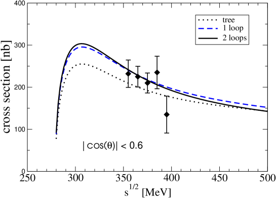
Figure 9: The cross-section of $\gamma\gamma\to\pi^{+}\pi^{-}$ with $|\cos\theta|\leq 0.6$ in the regime where ChPT is fully valid. The data are from Mark-II +citedataggpipi, the lowest order result is equivalent to scalar QED, the order $p^{4}$ result and order $p^{6}$ are from [63] and [71, 78]. Figure from Ref. [78].

The values of the polarizabilities are not in good agreement with the ChPT predictions, but there is a wide spread in the direct experimental values and the dispersive estimates. A discussion with more references can be found in [78] and [77]. Here I only quote the final result of order $p^{6}$ ChPT [78]

$$\left(\alpha_{1}-\beta_{1}\right)_{\pi^{\pm}}=(5.7\pm 1.0)\cdot 10^{-4}~{}\mathrm{fm}^{3}$$ (101)

and the result from the latest experiment [76]

$$\left(\alpha_{1}-\beta_{1}\right)_{\pi^{\pm}}=(11.6\pm 1.5_{\mathrm{stat}}\pm 3.0_{\mathrm{syst}}\pm 0.5_{\mathrm{mod}})\cdot 10^{-4}~{}\mathrm{fm}^{3}\,.$$ (102)

One sees that there is a clear, at present not understood, discrepancy. The ChPT prediction is not expected to have large corrections, it converged well and has good agreement with the direct data on $\gamma\gamma\to\pi^{+}\pi^{-}$. The experiment of [76] has also large contributions from the direct process $\gamma N\to\gamma N\pi$ and there might be ununderstood effects in the separation from the pion pole contribution.

3.5 Pion-pion scattering

Pion-pion scattering has received an enormous amount of attention both on the theoretical and experimental front. It is in some sense the most pristine of hadronic processes, involving only the lightest strongly interacting state. As mentioned earlier, the calculation by Weinberg in current algebra was one of the great successes of that approach in explaining the relative smallness compared to other strong interaction cross-sections.

The amplitude for pion-pion scattering can be written as

$$\langle\pi^{d}(p_{4})\pi^{c}(p_{3})\;\mbox{out}|\pi^{a}(p_{1})\pi^{b}(p_{2})\;\mbox{in}\rangle = \langle\pi^{d}(p_{4})\pi^{c}(p_{3})\;\mbox{in}|\pi^{a}(p_{1})\pi^{b}(p_{2})\;\mbox{in}\rangle$$ (103)

$$+i(2\pi)^{4}\delta^{4}(P_{f}-P_{i})\left\{\delta^{ab}\delta^{cd}A(s,t,u)+\mbox{cycl.}\right\}$$

where $s,t,u$ are the usual Mandelstam variables, expressed in units of the physical pion mass squared $M_{\pi}^{2}$,

$$s=(p_{1}+p_{2})^{2}/M_{\pi}^{2}\,,\quad t=(p_{3}-p_{1})^{2}/M_{\pi}^{2}\,,\quad u=(p_{4}-p_{1})^{2}/M_{\pi}^{2}\,.$$ (104)

Using these dimensionless quantities, the momentum expansion of the amplitude amounts to a Taylor series in

$${\it x_{2}}=\frac{M_{\pi}^{2}}{F_{\pi}^{2}}\,,$$ (105)

where $F_{\pi}$ denotes the physical pion decay constant.

The lowest order result was found by Weinberg using current algebra methods [42], the order $p^{4}$ calculation was performed by Gasser and Leutwyler [80]. The full calculation was done in [72, 54]. The result obtained there is

$$A(s,t,u) = \hskip 8.5359pt{\it x_{2}}\left[s-1\right]$$ (106)

$$+{\it x_{2}}^{2}\left[b_{1}+b_{2}s+b_{3}s^{2}+b_{4}(t-u)^{2}\right]$$

$$+{\it x_{2}}^{2}\left[F^{(1)}(s)+G^{(1)}(s,t)+G^{(1)}(s,u)\right]$$

$$+{\it x_{2}}^{3}\left[b_{5}s^{3}+b_{6}s(t-u)^{2}\right]$$

$$+{\it x_{2}}^{3}\left[F^{(2)}(s)+G^{(2)}(s,t)+G^{(2)}(s,u)\right]\,\!$$

$$+O({\it x_{2}}^{4})\,,$$

with

$${F^{(1)}}(\,{s}\,) = {\displaystyle\frac{1}{2}}\,\bar{J}(\,{s}\,)\,(\,{s}^{2}-1\,)\,,$$

$${G^{(1)}}(\,{s},{t}) = {\displaystyle\frac{1}{6}}\,\bar{J}(\,{t}\,)\,(14\,-\,4\,s\,-\,10\,t\,+\,s\,t\,+\,2\,t^{2}\,)\,,$$

$${F^{(2)}}(\,{s}\,) = \bar{J}(\,{s}\,)\left\{{\vrule height=7.89993pt,width=0.0pt,depth=7.89993pt}\right.\!\frac{1}{16\pi^{2}}\left(\!{\displaystyle\frac{503}{108}}\,{s}^{3}-{\displaystyle\frac{929}{54}}\,{s}^{2}+{\displaystyle\frac{887}{27}}\,{s}-{\displaystyle\frac{140}{9}}\right)$$

$$+ {b_{1}}\,(\,4\,{s}\,-3)+{b_{2}}\,(\,{s}^{2}+4\,{s}\,-4)$$

$$+ {\displaystyle\frac{{b_{3}}}{3}}\,\,(\,8\,{s}^{3}-21\,{s}^{2}+48\,{s}-32\,)+{\displaystyle\frac{{b_{4}}}{3}}\,(\,16\,{s}^{3}-71\,{s}^{2}+112\,{s}-48\,)\!\left.{\vrule height=7.89993pt,width=0.0pt,depth=7.89993pt}\right\}$$

$$+ \mbox{}{\displaystyle\frac{1}{18}}\,{K_{1}}(\,{s}\,)\,\left\{\!\!\,20\,{s}^{3}-119\,{s}^{2}+210\,{s}-135-{\displaystyle\frac{9}{16}}\,{\pi}^{2}\,(\,{s}-4\,)\,\!\right\}$$

$$+ \mbox{}{\displaystyle\frac{1}{32}}\,{K_{2}}(\,{s}\,)\,\left\{\!\,{s}\,{\pi}^{2}-24\,\!\right\}+{\displaystyle\frac{1}{9}}\,{K_{3}}(\,{s}\,)\,\left\{\,3\,{s}^{2}-17\,{s}+9\,\right\}\,,$$

$${G^{(2)}}(\,{s},{t}\,) = \bar{J}(\,{t}\,)\left\{{\vrule height=7.89993pt,width=0.0pt,depth=7.89993pt}\right.\!\frac{1}{16\pi^{2}}\left[{\displaystyle\frac{412}{27}}\!-\!{\displaystyle\frac{s}{54}}({t}^{2}+5\,{t}+159)\!-\!t\left(\frac{267}{216}{t}^{2}-\frac{727}{108}{t}+\frac{1571}{108}\right)\right]$$ (107)

$$+ {b_{1}}\,(2-{t})+{\displaystyle\frac{{b_{2}}}{3}}({t}-4)(2\,{t}+{s}-5)-{\displaystyle\frac{{b_{3}}}{6}}({t}-4)^{2}(3{t}+2{s}-8)$$

$$+ {\displaystyle\frac{{b_{4}}}{6}}\left(2{s}(3{t}-4)({t}-4)-32t+40t^{2}-11{t}^{3}\,\right)\!\left.{\vrule height=7.89993pt,width=0.0pt,depth=7.89993pt}\right\}\mbox{}$$

$$+ {\displaystyle\frac{1}{36}}{K_{1}}(\,{t}\,)\left\{\,174+8\,{s}-10\,{t}^{3}+72\,{t}^{2}-185\,{t}-{\displaystyle\frac{{\pi}^{2}}{16}}\,(\,{t}-4\,)\,(\,3\,{s}\!-\!8\,)\,\!\right\}$$

$$+ \mbox{}{\displaystyle\frac{1}{9}}\,{K_{2}}(\,{t}\,)\,\left\{\!\,1+4\,{s}+{\displaystyle\frac{{\pi}^{2}}{64}}\,{t}\,(\,3\,{s}-8\,)\ \,\!\right\}$$

$$+ {\displaystyle\frac{1}{9}}\,{K_{3}}(\,{t}\,)\left\{1+3{s}{t}-{s}+3{t}^{2}-9{t}\right\}+{\displaystyle\frac{5}{3}}\,{K_{4}}(\,{t}\,)\,\left\{\,4-2\,{s}-{t}\,\right\}\,.$$

The loop functions $\bar{J}$ and $K_{i}$ are

$$\left(\begin{array}[]{l}\bar{J}\\ K_{1}\\ K_{2}\\ K_{3}\\ \end{array}\right)=\left(\begin{array}[]{cccc}0&0&z&-4N\\ 0&z&0&0\\ 0&z^{2}&0&8\\ Nzs^{-1}&0&\pi^{2}(Ns)^{-1}&\pi^{2}\\ \end{array}\right)\left(\begin{array}[]{c}{h}^{3}\\ {h}^{2}\\ {h}\\ \displaystyle{-(2N^{2})^{-1}}\end{array}\right)\,,$$

and

$$K_{4} = \frac{1}{sz}\left(\frac{1}{2}K_{1}+\frac{1}{3}K_{3}+\frac{1}{N}\bar{J}+\frac{(\pi^{2}-6)s}{12N^{2}}\right)\,,$$

where

$${h}(s)=\frac{1}{N\sqrt{z}}\ln\frac{\sqrt{z}-1}{\sqrt{z}+1}\quad,\qquad z=1-\frac{4}{s}\;,\;N=16\pi^{2}\,.$$

The functions $s^{-1}\bar{J}$ and $s^{-1}K_{i}$ are analytic in the complex $s$–plane (cut along the positive real axis for $s\geq 4$), and they vanish as $|s|$ tends to infinity. Their real and imaginary parts are continuous at $s=4$. The coefficients $b_{i}$ in the polynomial part are given in App. D of [54] and their dependence on the $p^{6}$ LECs can be found in [53].

A few comments are in order here. The result (106) can be rewritten in the form derived in [61]. The relevant loop-integrals can all be written in terms of elementary functions. This is a feature of many of the results when all masses are equal but not for all. The ChPT series in fact converges reasonably well as can be seen in Fig. 10.

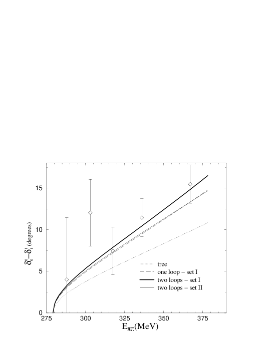
Figure 10: The pion-pion phase-shift difference $\delta_{0}^{0}-\delta_{1}^{1}$ as a function of the center-of-mass energy. Shown are the lowest order, order $p^{4}$ and order $p^{6}$. The latter is shown for two sets of input parameters together with the then most precise data [81]. Figure from Ref. [54].

This is a review on ChPT but some of the recent history in the theoretical treatment of pion-pion scattering deserves mention. The Roy equations [82] have been reanalyzed in great detail in Ref. [83]. A similar analysis was also performed in [84]. The results of this analysis have been combined with the results of the order $p^{6}$ calculation mentioned here to get a series of very precise predictions for the pion-pion scattering system in [85, 86]. These predictions have been nicely confirmed by experiment [87, 88] and [89]. The relevance for the mechanism of spontaneous symmetry breaking in QCD is discussed in [86]. The case with a possible small value of the quark condensate [41] is now ruled out.

The work of [83, 85, 86] has been criticized in Refs. [90, 91] on two grounds, the high-energy input used as well as the fact that certain sum-rules were not obeyed by the results of [83, 85, 86]. The criticisms in these papers have been answered in Refs. [92, 93]. They showed that the high-energy input used in [83, 85, 86] also satisfied the requirements as well as the one advocated in [90, 91]. They showed as well that changing the high-energy input to the one of [90, 91] did not change their result outside quoted errors. The sum-rules discussed in [90, 91] are not well convergent. Ref. [92, 93] showed that more convergent versions of the sum-rules are well satisfied by their results.

The successful prediction of pion-pion scattering at low-energy from the combination of ChPT and Roy equations is one of the great successes of theory in low-energy hadronic physics.

3.6 Pion form-factors

The pion vector and scalar form-factors are also known analytically to order $p^{6}$ [73]. They are defined respectively by

$$\langle\pi^{i}(p_{2})|\bar{u}u+\bar{d}d|\pi^{j}(p_{1})\rangle = \delta^{ij}F_{S}(s_{\pi})\;,$$

$$\langle\pi^{i}(p_{2})|\frac{1}{2}\left(\bar{u}\gamma_{\mu}u-\bar{d}\gamma_{\mu}d\right)|\pi^{j}(p_{1})\rangle = i\varepsilon^{i3j}(p_{1\mu}+p_{2\mu})F_{V}(s_{\pi})\;,$$ (109)

where $s_{\pi}=(p_{2}-p_{1})^{2}$. The scalar form-factor is defined with an isospin–zero scalar source. The isospin–one scalar form-factor can be defined analogously but it only starts at ${\cal O}(p^{4})$. The vector form factor is here defined as the isovector part only, and what we calculate here is its $I_{z}=0$ component. Similar definitions exist for the other isospin components. In the limit of conserved isospin, these components are the relevant ones. The tree level results have been long known and it is one for the vector form-factor. The order $p^{4}$ result has been derived in Ref. [2] and the full order $p^{6}$ expressions have been obtained by the authors of Ref. [73]. Similar to the case of pion-pion scattering, the expressions are fully given in terms of elementary functions.

The two form-factors have a different behaviour. The vector form-factor has relatively small corrections coming from the loop diagrams and has the corrections dominated by the part given by the LECs of order $p^{4}$ and $p^{6}$. The fit to data is dominated by the spacelike measurements of the pion form-factor at CERN by NA7. In Fig. 11 we have shown the quality of the fit achieved.

Figure 11: The spacelike vector form-factor of the charged pion and the best fit of the ChPT order $p^{6}$ expression enhanced by a cubic analytic term. Figure from Ref. [73].

This fit also allowed for a good measurement of a $p^{4}$ and $p^{6}$ LEC. The result is [73]

$$\bar{l}_{6} = 16.0\pm 0.5\pm 0.7\,,$$

$$r^{r}_{V2}(M_{\rho}) = -4c^{r}_{51}+4c^{r}_{53}=(1.6\pm 0.5)\cdot 10^{-4}\,.$$ (110)

For the pion scalar form-factor there is no direct experimental information. The momentum dependence can be derived using dispersive methods [94]. More recent determinations and discussion using the same method can be found in [95, 96, 97]. The result for the $p^{4}$ LEC that follows from a reasonable range for the scalar radius is

$$\bar{l}_{4}=4.4\pm 0.3$$ (111)

if one assumes a range for the scalar radius

$$\langle r^{2}\rangle_{S}^{\pi}=0.60\pm 0.03~{}\mathrm{fm}^{2}\,.$$ (112)

An approximate value for an order $p^{6}$ constant could also be obtained from this comparison, but its actual value was dependent on the other $p^{4}$ LECs input values used. Ref. [73] obtained

$$r_{S3}^{2}=-8c^{r}_{6}\approx 1.0\cdot 10^{-4}\,.$$ (113)

3.7 $\pi\to\ell\nu\gamma$

The last full calculation in two-flavour ChPT to order $p^{6}$ I am aware of is for the radiative decay of the pion in Ref. [98]. The process $\pi^{+}\to\ell^{+}\nu\gamma$ at lowest order is nothing but the QED correction to the pointlike $\pi\to\ell\nu$ decay. First at order $p^{4}$ are there contributions from the pion structure and the allow a sizable effect for $\pi^{+}\to e^{+}\nu\gamma$ since the QED Bremsstrahlung contribution is helicity suppressed there.

The order $p^{4}$ contribution has been calculated in Ref. [2]. The order $p^{6}$ calculation was added in Ref.[98]. Again, a rather good convergence from the order $p^{4}$ to the order $p^{6}$ result was seen. The combination of order $p^{4}$ LECs that can be obtained from this calculation is [98]

$$2l_{5}-l_{6}=0.00315\pm 0.00030\,.$$ (114)

This was derived from the value for the axial form-factor in the decay. There have since been new data from the PIBETA collaboration [99] which are compatible with the value of the axial form-factor used in [73] to determine (114). Note that the general agreement of the data with the distributions predicted by ChPT, or the standard $V-A$ picture is not very good. The variation of the form-factors with momenta is expected to be small and the experimental variation is significant, alternatively other form-factors can contribute. This discrepancy is at the edge of statistical significance as discussed in [99].

3.8 Values of the low-energy constants

The LECs of order $p^{4}$ were first determined in the original paper [2] using the then best values and the order $p^{4}$ expressions that were derived there as well. All these quantities are now known to order $p^{6}$ which in principle allows for a much more precise determination. A problem that surfaces at this level is how to deal with the values of the unknown order $p^{6}$ LECs. In all of the papers mentioned earlier similar estimates using resonance saturation have been used. Since quark-mass corrections in the two-flavour case are suppressed by powers of $M_{\pi}^{2}$ the unknown parameters have typically a fairly small effect but no general study of this has been undertaken.

The best estimate of $\bar{l}_{1}$ to $\bar{l}_{4}$ comes from the combination of ChPT at order $p^{6}$ and the Roy equation analysis of Ref.[86]. The other two known parameters are $\bar{l}_{5}$ and $\bar{l}_{6}$ as discussed earlier. The best values at present are thus

$$\bar{l}_{1} = -0.4\pm 0.6\,,$$

$$\bar{l}_{2} = 4.3\pm 0.1\,,$$

$$\bar{l}_{3} = 2.9\pm 2.4\,,$$

$$\bar{l}_{4} = 4.4\pm 0.2\,,$$

$$\bar{l}_{6}-\bar{l}_{5} = 3.0\pm 0.3\,,$$

$$\bar{l}_{6} = 16.0\pm 0.5\pm 0.7\,.$$ (115)

The value for $\bar{l}_{4}$ is in complete agreement with the one in Eq. (111). The error is smaller due to the fact that the work of [86] allowed to pin down some of the input better than in [73]. The remaining parameter $l_{7}$ is not known directly from phenomenology. It can in principle be determined from lattice QCD evaluations of the neutral pion mass in the presence of isospin breaking. Its value was estimated to be about

$$l_{7}\sim 5\cdot 10^{-3}$$ (116)

from $\pi^{0}$-$\eta$ mixing in [2].

Some combinations of order $p^{6}$ LECs are known as well. Two have been derived from the vector and scalar form-factor of the pion and have been given above. Ref. [86] has derived some more combinations which are implicit in the values of $b_{5}$ and $b_{6}$ quoted there.

4 Three-flavour calculations

The three-flavour calculations started soon after the first two-flavour results had appeared. In the two-flavour case all calculations have used the same renormalization procedure as discussed in Sect. 2.10 with the ChPT modified version of modified minimal subtraction. This is unfortunately not true for the three-flavour case where at least three different renormalization schemes have been used. These schemes are related and can in principle be related to each other. In practice it has made use of calculations of different groups of authors difficult. The situation at present is that most calculations performed by Bijnens and collaborators have been used together with a similar scheme of analysis and the standard ChPT subtraction scheme. Most of the other calculations have done only a rather small amount of numerical analysis, often using a set of LECs determined at order $p^{4}$.

In this section I give a list of the calculations which have been done and show a few typical numerical results. The section finishes with a discussion of how the order $p^{6}$ LECs have been treated in the existing calculations and I also briefly discuss more recent developments which have happened in this regard.

4.1 The vector two-point functions

The vector currents are defined as

$$V_{\mu}^{ij}(x)=\overline{q}^{i}\gamma_{\mu}q^{j}\;,$$ (117)

where the indices $i$ and $j$ run over the three light quark flavours, $u$, $d$ and $s$. Working in the isospin limit all SU(3) currents can be constructed using isospin relations from

$$V_{\mu}^{\pi}(x) = \frac{1}{\sqrt{2}}\left(V_{\mu}^{11}(x)-V_{\mu}^{22}(x)\right)\,,$$

$$V_{\mu}^{\eta}(x) = \frac{1}{\sqrt{6}}\left(V_{\mu}^{11}(x)+V_{\mu}^{22}(x)-2V_{\mu}^{33}(x)\right)\,,$$

$$V_{\mu}^{K}(x) = V_{\mu}^{31}(x)\;.$$ (118)

These will be referred to as the isospin or pion, hypercharge or eta and kaon vector currents respectively. All others can be defined from these in the isospin limit. E.g. the electromagnetic current corresponds to

$$V_{\mu}^{{em}}=\frac{e}{\sqrt{2}}V_{\mu}^{\pi}(x)+\frac{e}{\sqrt{6}}V_{\mu}^{\eta}(x)\;.$$ (119)

The two-point functions are defined in terms of the currents as

$$\Pi_{\mu\nu}^{Va}(q)\equiv i\int d^{4}x\;e^{iq\cdot x}\;\langle 0|T(V_{\mu}^{a}(x)V_{\nu}^{a}(0))^{\dagger}|0\rangle\,,$$ (120)

for $a=\pi,\eta,K$. All other vector two-point functions can be constructed from these using isospin relations. Lorentz-invariance allows to express them in a transverse, $\Pi^{(1)}$, and a longitudinal, $\Pi^{(0)}$, part via

$$\Pi_{\mu\nu}^{Va}=(q_{\mu}q_{\nu}-q^{2}g_{\mu\nu})\Pi_{Va}^{(1)}(q^{2})+q_{\mu}q_{\nu}\Pi_{Va}^{(0)}(q^{2})\;.$$ (121)

For a conserved current, which is the case for the pion and eta current, the longitudinal part vanishes because of the Ward identities.

These two-point functions were first evaluated in Ref. [100] for the isospin and hypercharge, i.e. the diagonal, vector-currents. The missing case for the vector-current with Kaon quantum numbers was later added by Ref. [101] and [102]. The relevant diagrams to order $p^{6}$ are shown in Fig. 12. There is no order $p^{2}$ contribution, the order $p^{4}$ diagrams are the first line, (a-c), and the remainder are the order $p^{6}$ diagrams.

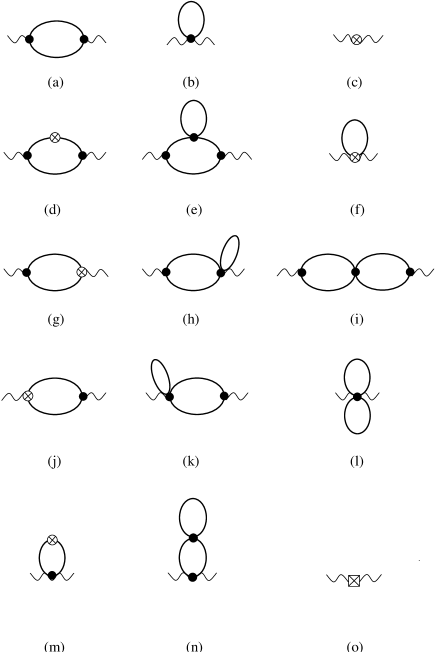
Figure 12: The Feynman diagrams needed to calculate the vector two-point functions at order $p^{6}$. The crossed circle stands for the order $p^{4}$ vertex insertion. Wiggly lines are the external vector currents. Dots are order $p^{2}$ vertices and a square is an order $p^{6}$ vertex. The solid lines are meson propagators. Figure from Ref. [101].

There are no proper two-loop integrals needed to evaluate the vector two-point functions to order $p^{6}$. They have not been used very much for phenomenological purposes but could in principle be used as low-energy constraints on sum-rule analyses in this channel. Some results were given in Ref. [100]. The papers [101] and [100, 102] used a different subtraction scheme so a full comparison has not been done, but the checked parts are in agreement between the two independent evaluations.

The isospin breaking vector two-point function was calculated to order $p^{6}$ in Ref. [103] and were used as constraints in a sum-rule analysis of isospin breaking in vector meson decay constants [104].

4.2 Scalar two-point functions

The scalar two-point functions can be calculated from a similar set of diagrams as the vector two-point functions by replacing the insertion of the vector currents in Fig. 12 by scalar currents. The main one used in this sector is

$$\Pi^{S}(q)\equiv i\int d^{4}x\;e^{iq\cdot x}\;\langle 0|T((S^{uu}(x)+S^{dd}(x))S^{ss}(0)^{\dagger}|0\rangle\,,$$ (122)

with the scalar densities $S^{ij}$ defined in Eq. (2.2). It was calculated to order $p^{6}$ by Moussallam [105] and used in an analysis to obtain bounds on $L_{6}^{r}$.

4.3 Quark condensates

Another quantity which can be evaluated without proper two-loop integrals at order $p^{6}$ is the quark condensate

$$\langle\overline{q}^{i}q^{j}\rangle.$$ (123)

It has been evaluated in the isospin limit in Ref. [106] and the isospin breaking corrections in Ref. [107] for the three possible cases $i=j=u,d,s$.

The value of the quark condensate depends on the constant $H_{1}^{r}$ at order $p^{4}$. This cannot be directly measured in any physical process. It’s value depends on the precise definition of the quark densities in QCD. To order $p^{6}$ the local counterterms of that order also contribute to $\langle\overline{q}^{i}q^{j}\rangle$. The corrections when $L_{4}^{r}$ and $L_{6}^{r}$ are assumed to be zero are fairly small as can be seen from the plots in Ref. [106] for $\langle\overline{u}u\rangle$ and $\langle\overline{d}d\rangle$ but they were sizable for $\langle\overline{s}s\rangle$.

As discussed shortly in Sect. 3 it is now clear that the quark condensate in the two-flavour case remains large also in the chiral limit where $m_{u}$ and $m_{d}$ are sent to zero. The equivalent question for the three-flavour chiral limit remains open as discussed in [95] and [36, 108]. The situation here is analogous to the situation in the two-flavour case before the latest results on pion-pion scattering threshold parameters, all results seem to indicate that the standard picture as described in this review is consistent but an alternative scenario is not ruled out. The main remaining obstacle in the three flavour case is that the effects of the order $p^{6}$ LECs have not been constrained in sufficient detail yet to see how this question can be resolved. Work is ongoing whether the results for $\pi\pi$ and $\pi K$ scattering can be sufficiently refined theoretically to provide such a test.

4.4 Axial-vector two-point functions, masses and decay-constants

These are the simplest quantities requiring proper two-loop integrals. The axial-vector currents are defined as

$$A_{\mu}^{ij}(x)=\overline{q}^{i}\gamma_{\mu}\gamma_{5}q^{j}$$ (124)

where the indices $i$ and $j$ run over the three light quark flavours, $u$, $d$ and $s$. Working in the isospin limit all SU(3) currents can be constructed using isospin relations from

$$A_{\mu}^{\pi}(x) = \frac{1}{\sqrt{2}}\left(V_{\mu}^{11}(x)-V_{\mu}^{22}(x)\right)\,,$$

$$A_{\mu}^{\eta}(x) = \frac{1}{\sqrt{6}}\left(V_{\mu}^{11}(x)+V_{\mu}^{22}(x)-2V_{\mu}^{33}(x)\right)\,,$$

$$A_{\mu}^{K}(x) = V_{\mu}^{31}(x)\;.$$ (125)

These will be referred to as the isospin or pion, hypercharge or eta and kaon axial-vector currents respectively. All others can be defined from these in the isospin limit.

The two-point functions are defined in terms of the currents as

$$\Pi_{\mu\nu}^{Aa}(q)\equiv i\int d^{4}x\;e^{iq\cdot x}\;\langle 0|T(A_{\mu}^{a}(x)A_{\nu}^{a}(0))^{\dagger}|0\rangle\,,$$ (126)

for $a=\pi,\eta,K$. Using isospin relations, all other axial-vector two-point functions can be constructed from these using isospin relations. Lorentz-invariance allows to express them in a transverse, $\Pi^{(1)}$, and a longitudinal, $\Pi^{(0)}$, part

$$\Pi_{\mu\nu}^{Aa}=(q_{\mu}q_{\nu}-q^{2}g_{\mu\nu})\Pi_{Aa}^{(1)}(q^{2})+q_{\mu}q_{\nu}\Pi_{Aa}^{(0)}(q^{2})\;.$$ (127)

The axial currents are only conserved in the chiral limit, i.e. when the masses of all quarks in the currents involved vanish. Thus in general there is both a longitudinal and a transverse part.

The axial-vector two-point functions have contributions from one-particle-reducible diagrams, those where the cutting of one line makes the diagram become disconnected. The full set is shown in Fig. 13.

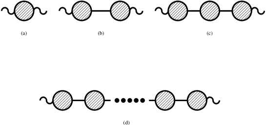
Figure 13: The diagrams contributing to the axial-vector two-point function. The filled circles indicate the one-particle-irreducible (1PI) diagrams. Solid lines are pseudoscalar meson propagators and the wiggly lines indicate insertions of an axial-vector current. For the inverse propagator the wiggly lines are meson legs and for the decay constant the right wiggly line is a meson leg while the left remains an axial current. Figure from Ref. [101].

The filled circles in Fig. 13 are the sum of all 1PI diagrams. Those up to order $p^{6}$ are shown in Fig. 14.

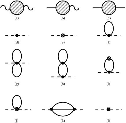
Figure 14: The set of diagrams contributing to the 1PI quantities. (a) axial-vector–axial-vector (b) axial-vector–pseudoscalar (c) pseudoscalar–pseudoscalar. (d)-(l) the respective diagrams when the dashed lines are replaced with the external legs of (a), (b) or (c). A line is a meson propagator, a wiggly line an external source, a dot a vertex of order $p^{2}$, a crossed circle a vertex of order $p^{4}$ and a crossed box a vertex of order $p^{6}$. Figure from Ref. [101].

The diagram in Fig. 14(k), the so-called sunset diagram is the first diagram we encounter in this section that requires the evaluation of proper two-loop integrals. Methods to perform these integrals thus needed to be developed. The methods derived in [68] need to be generalized to the case with different masses in the loop. An efficient method to get the sunset diagram at zero momentum was derived in Ref. [109] using recursion relations between the various integrals. A different derivation of the same relations was presented in Ref. [101]. The method for the momentum dependence of the sunsetintegrals of [68] was extended to the different mass case in [101]. Ref. [110] used a different variation on the sunset integral method of [68] to perform their numerical analysis.

In Ref. [110] the axial-vector two-point function with pion and eta quantum numbers was evaluated to order $p^{6}$. They also used this to evaluate the pion and eta masses and decay constants as well as a simple sum-rule analysis [111]. The axial-vector two-point functions were calculated also in Ref. [101] where the same quantities with kaonic quantum numbers were also evaluated to order $p^{6}$. At this level all masses and decay constants were known in the isospin limit. Note that the masses can be calculated from the position of the pole in the full propagator and the decay constant by direct evaluation of the matrix element

$$\langle 0|A^{a}_{\mu}|M(p)\rangle=i\sqrt{2}F_{M}P_{\mu}\,.$$ (128)

$F_{M}^{2}$ can be determined as well from the residue of the meson pole in the longitudinal part of the axial-vector two-point function. That all these methods of calculating the masses and the decay constants give the same answer was explicitly checked in Ref. [101].

What was found for the masses was that the order $p^{4}$ corrections were small for the standard set of input parameters from fits at order $p^{4}$, see Ref. [112] for this determination. However, the order $p^{6}$ corrections were rather large for both [110] and [106]. It should be noted that there was analytical agreement between those two references for the parts that could be checked without relating the different renormalization schemes and the different way of evaluating the integrals. At present there is no obvious solution for the presence of these large corrections. It is possible to choose the order $p^{6}$ LECs to cancel these corrections but the LECs involved are those coming from the scalar sector and are the most difficult ones to estimate. The naive estimates used in [101] gave a very large range for the contribution from the order $p^{6}$ LECs, from extremely large to zero. In Sect. 4.8 I will discuss a few more relevant results.

The masses and decay constants away from the isospin limit have also been worked out. These calculations were reported in Ref. [107].

4.5 $K_{\ell 4}$

The decay $K\to\pi\pi\ell\nu$ was first treated using current algebra methods to obtain the lowest order result. The order $p^{4}$ calculation was performed by two groups simultaneously [113, 114] with complete analytical agreement. The reason for calculating this decay beyond lowest order was two-fold. The most accurate determinations of the form-factors showed a significant deviation from the lowest order prediction. It was expected that the order $p^{4}$ calculation would allow to fit the experimental results and allow for a more accurate determination of $L_{i}^{r}$ with $i=1,2,3$.

The corrections to the lowest order were of the expected order but not very small. This prompted an investigation of higher orders using dispersive methods. This was done in Ref. [115]. In that reference also the missing form-factor $R$ defined below was evaluated to order $p^{4}$. The higher order corrections were of the expected order indicating a converging series for this decay. The fit results of Ref. [115] have been the standard set of values for the order $p^{4}$ LECs replacing the earlier full fit of Ref. [3].

When the full work on pion-pion scattering in two-flavour ChPT was finished it became interesting to check whether this calculation was compatible with the values of the order $p^{4}$ LECs determined from $K_{\ell 4}$. To be able to do this $K_{\ell 4}$ needed to be determined also to order $p^{6}$. This calculation was performed by the authors of Ref. [106, 116]. I will now present the results from these references.

The $K_{\ell 4}$ decay processes are

$$K^{+}(p) \to \pi^{+}(p_{+})\pi^{-}(p_{-})\ell^{+}(p_{\ell})\nu_{\ell}(p_{\nu})\,,$$

$$K^{+}(p) \to \pi^{0}(p_{+})\pi^{0}(p_{-})\ell^{+}(p_{\ell})\nu_{\ell}(p_{\nu})\,,$$

$$K^{0}(p) \to \pi^{-}(p_{+})\pi^{0}(p_{-})\ell^{+}(p_{\ell})\nu_{\ell}(p_{\nu})\,.$$ (129)

The corresponding momenta are given inside the brackets after each particle. Following the original work [117], the $K_{\ell 4}$ decays are parameterized in terms of five kinematical variables:
i) $s_{\pi}$, the squared effective mass of the dipion system.
ii) $s_{\ell}$, the squared effective mass of the dilepton system.
iii) $\theta_{\pi}$, the angle between the $\pi^{+}$ and the dipion line of flight with respect to the Kaon rest frame.
iv) $\theta_{\ell}$, the angle between the $\ell^{+}$ and the dilepton line of flight with respect to the Kaon rest frame.
v) $\phi$, the angle between the $\pi-\pi$ and $e-\nu$ planes with respect to the Kaon rest frame.

However, from the point of view of the hadronic system alone, a better choice of variables is to use in addition to $s_{\pi}$, $\cos\theta_{\ell}$ and $\phi$, also

$$t_{\pi}=(p_{+}-p)^{2}\quad\mbox{and}\quad u_{\pi}=(p_{-}-p)^{2}\,,$$ (130)

related through

$$s_{\pi}+t_{\pi}+u_{\pi} = m_{K}^{2}+2\,m_{\pi}^{2}+s_{\ell}\,,$$

$$t_{\pi}-u_{\pi} = -2\sigma_{\pi}X\cos\theta_{\pi}\,,$$ (131)

with

$$X = \frac{1}{2}\lambda^{1/2}(m_{K}^{2},s_{\pi},s_{\ell})\,,$$

$$\sigma_{\pi} = \sqrt{1-4m_{\pi}^{2}/s_{\pi}}\,,$$

$$\lambda(m_{1},m_{2},m_{3}) = m_{1}^{2}+m_{2}^{2}+m_{3}^{2}-2\,(m_{1}m_{2}+m_{1}m_{3}+m_{2}m_{3})\,.$$ (132)

With the previous notation the amplitude for the decay $K^{+}\rightarrow\pi^{+}\pi^{-}\ell^{+}\nu_{\ell}$ is

$$T^{+-}=\frac{G_{F}}{\sqrt{2}}V^{*}_{us}\overline{u}(p_{\nu})\gamma_{\mu}(1-\gamma_{5})v(p_{\ell})(V^{\mu}-A^{\mu})\;,$$ (133)

with

$$V_{\mu} = -\frac{H}{m^{3}_{K}}\epsilon_{\mu\nu\rho\sigma}(p_{\ell}+p_{\nu})^{\nu}(p_{+}+p_{-})^{\rho}(p_{+}-p_{-})^{\sigma}\;,$$

$$A_{\mu} = -\frac{i}{m_{K}}[(p_{+}+p_{-})_{\mu}\;F+(p_{+}-p_{-})_{\mu}\;G+(p_{\ell}+p_{\nu})_{\mu}\;R]\;.$$ (134)

$V_{us}$ is the relevant CKM matrix-element. The other two amplitudes, $T^{-0}$ and $T^{00}$, are defined similarly.

Here we are interested in the $F$ and $G$ form-factors. The $H$ form-factor is known to ${\cal O}(p^{6})$ [118] and the $R$ form-factor always appears with a factor of $m_{\ell}^{2}$ and its contribution negligible for the electron case. $R$ is known to order $p^{4}$ [115]. The form-factors are functions of $s_{\pi}$, $s_{\ell}$ and $\cos\theta_{\pi}$ only, or alternatively of $s_{\pi}$, $t_{\pi}$ and $u_{\pi}$.

The relations between the form-factors and the intensities, easier to obtain from the experiment, can be found in [119] or in [115].

The amplitudes for the three processes of Eq. (4.5) are related using isospin by

$$T^{+-}=\frac{T^{-0}}{\sqrt{2}}+T^{00}$$ (135)

with $T^{ij}$ the matrix element defined in Eq. (133). $T^{-0}$ is anti-symmetric under the interchange of the pion momenta while $T^{00}$ is symmetric. This also implies relations between the form-factors themselves. Observe the different phase convention in the isospin states compared to [115] where $M^{00}$ appears with a minus sign because of the Condon–Shortley phase convention.

The form-factors $F$ and $G$ can be decomposed in partial waves. The partial wave expansion is not simply for $F$ and $G$ since the components with a well defined $L_{z}=0,\pm 1$ need to be expanded [117, 119]. The relevant expressions can be found in [117, 119, 115, 106] and a discussion of their relative sizes and how they can be used in experiment is in the mentioned references but more elaborated in Ref. [120]. I will not go further into this but simply quote the experimental results.

The lowest order calculation was done using current algebra methods by Weinberg [121]. Both the $F$ and $G$ form-factor are equal and given by a single insertion of a ${\cal L}_{2}$ vertex in diagram (a) of Fig. 15. The result is

$$F=G=\frac{m_{K}}{\sqrt{2}F_{\pi}}\,,$$ (136)

where $m_{K}$ is the physical Kaon mass. At higher orders more diagrams become relevant. The tree-level and one-loop diagrams are shown in Fig. 15. To order $p^{4}$ we need in addition the diagram of Fig. 15(a) but with an order $p^{4}$ vertex as well as the loop diagrams (b,c) of the same figure with only order $p^{2}$ vertices. With order $p^{4}$ result, the experimental data at he time can be nicely fitted, as discussed extensively in Ref. [114] and later in Ref. [115].

The diagrams at order $p^{6}$ that are relevant for the calculation of the $F$ and $G$ form-factors defined in Eq. 4.5 are shown in Figs. 16 and 16 in addition to diagrams in Fig. 15 with insertions of an order $p^{6}$ vertex in diagram (a) or one order $p^{4}$ vertex in (b,c). The diagrams shown in Fig. 16 do not require any proper two-loop integrals. They can be calculated using straightforward methods and only present difficulties due to the length of the expressions.

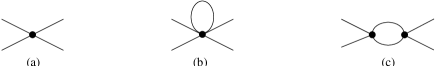
Figure 15: (a) One-particle irreducible tree level diagram. (b) One-particle irreducible one-loop diagrams. Dots refer to strong vertices or current insertions from ${\cal L}_{2}$, ${\cal L}_{4}$ or ${\cal L}_{6}$. External legs stand for pseudoscalar or weak current. Internal lines are pseudoscalars only. Figure from Ref. [106].

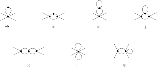
Figure 16: One-particle irreducible order $p^{6}$ diagrams with only one-loop integrals. The dots are order $p^{2}$ vertices except the top dot in (d) and (e) which is an order $p^{4}$ vertex. In addition there are the diagrams (b) and (c) of Fig. 15 with one of the dots replaced by a ${\cal O}(p^{4})$ vertex. Figure from Ref. [106].

Proper two-loop integrals show up in the diagrams shown in Fig. 17. The left one, (a), is called the sunset-diagram and the integrals needed are the sunsetintegrals. These were discussed briefly in Sect. 4.4. The diagram on the right-hand-side, (b), in Fig. 17 is the single most difficult diagram in this calculation. It is called the vertex-diagram or sometimes the fish-diagram. There have been quite a few different methods used to evaluate this type in integrals in order $p^{6}$ calculations. The one used in most calculations is based on the work of Ghinculov, van der Bij and Yao [122] and can be found in those references or in Ref. [123].

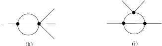
Figure 17: One-particle irreducible order $p^{6}$ diagrams with irreducible two-loop integrals. The dots are order $p^{2}$ vertices. Figure from Ref. [106].

In addition to the diagrams shown in Figs. 15-17, there is the contribution from wave-function renormalization from the diagrams shown in Fig. 14. The order $p^{6}$ expressions are very long and are partly reported in a numerical parameterization only in Ref. [106]. It was found that the parameterization based on a truncated partial wave expansion as proposed in Ref. [120] worked very well.

To show the results, we first compare the Omnès improved order $p^{4}$ result of Ref. [115] together with the data of Ref. [81] in Fig. 18. The result was fitted to that data so there is quite good agreement. However, when we compare the full order $p^{6}$ calculation we notice that there is quite a difference with the dispersive, i.e. the Omnès improved, estimate. We also see a reasonable convergence of $F$ going from order $p^{2}$ to $p^{4}$ to $p^{6}$.

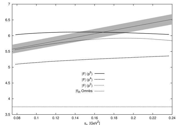
Figure 18: Comparison of the Omnès improved estimate of Ref. [115] with the full order $p^{6}$ of calculation of Ref. [106] using the same set of values of $L_{i}^{r}$ as input together with $F_{\pi}=93.2$ MeV. The shaded band is the experimental result of [81]. Figure from Ref. [106].

After performing a fit to the data of Rosselet et al. [81], the order $p^{6}$ result fits the data nicely. The resulting different orders are shown in Fig. 19. For both form-factors there is a good convergence. The estimate of the contributions of the order $p^{6}$ Lagrangian, the curve labeled $C_{i}^{r}$-only, is also shown. It is small for both form-factors. The estimate for $G$ is somewhat larger, but follows from measured resonance decays so it is fairly certain. The full description of how this estimate has been done can be found in Refs. [115, 106].

Another feature visible in the figures is that for $F$, which is dominated by the $S$-wave, final state rescattering is rather important since the contribution from the imaginary part to $|F|$ is quite visible. In contrast, $G$ is dominated by the $P$-wave and final state rescattering effects are fairly small.

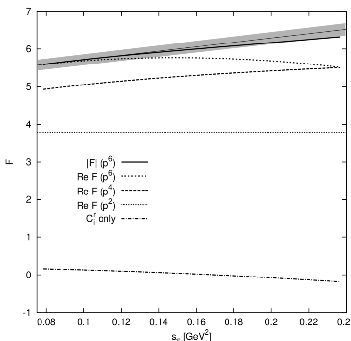
(a)

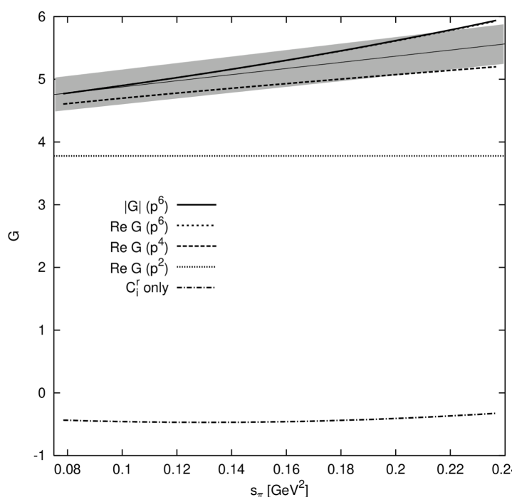
(a)

Figure 19: The $F$ (a) and $G$ (b) form-factor at $s_{\ell}=0$ and $\cos\theta_{\pi}=0$. The shaded band is the result of [81]. Shown are the full result for the absolute value, and the real part to lowest-order, ${\cal O}(p^{4})$ and ${\cal O}(p^{6})$. We also show the contribution from the ${\cal O}(p^{6})$ Lagrangian; this is dominated by the vector contribution. The curves for Re $G$ and $|G|$ are very close since Im $G$ is very small. Figure from Ref. [106].

After the work of Ref. [106] was finished, new data have appeared. The main new data from the BNL experiment [87, 88] were included in the full fit done in Ref. [107]. These data were preliminary at the time, so they were not called the main fit in that reference. The best fit, including the newer data, is called “fit 10” in Ref. [107] and is the one which has been used in most works following it.

In Ref. [106], a study of the dependence on the constants $L_{4}^{r}$ and $L_{6}^{r}$ was done as well. A main goal was to see whether good fits could be obtained with these at values different from zero as well. It was found that such is indeed the case, and that in order to obtain these two order $p^{4}$ constants, additional experimental input was needed. This will be discussed in the context of the scalar form-factors, pion-pion and pion-kaon scattering below.

We also expect that new data on various $K_{\ell 4}$ decays will become available from the NA48 experiment.

4.6 Vector or electromagnetic form-factors

The most general structure for the on-shell pseudoscalar-pseudoscalar-vector Green function is dictated by Lorentz invariance. With the additional use of charge conjugation and electromagnetic gauge invariance one can parameterize the pion and kaon electromagnetic matrix elements as

$$\langle\pi^{+}(q)|j_{\mu}|\pi^{+}(p)\rangle = (q_{\mu}+p_{\mu})F^{\pi}_{V}(t)\,,$$

$$\langle K^{+}(q)|j_{\mu}|K^{+}(p)\rangle = (q_{\mu}+p_{\mu})F^{K^{+}}_{V}(t)\,,$$

$$\langle K^{0}(q)|j_{\mu}|K^{0}(p)\rangle = (q_{\mu}+p_{\mu})F^{K^{0}}_{V}(t)\,,$$ (137)

with $t=(q-p)^{2}$. The current $j_{\mu}$ refers to the electromagnetic current of the light flavours

$$j_{\mu}=\frac{2}{3}\left(\bar{u}\gamma_{\mu}u\right)-\frac{1}{3}\left(\bar{d}\gamma_{\mu}d+\bar{s}\gamma_{\mu}s\right)\,.$$ (138)

The quantities $F_{V}^{\pi},F_{V}^{K^{0}}$ and $F_{V}^{K^{+}}$ will be referred to hereafter as the vector form-factors or simply the form-factors. They are also defined in the crossed channel $\langle 0|j_{\mu}|M^{a}(p)M^{b}(-q)\rangle$.

To lowest order the vector form-factors are constant and are simply the charge of the relevant meson under the current under consideration. The order $p^{4}$ calculation was performed by Gasser and Leutwyler in Ref. [124] and confirmed for the pion form-factor in Ref. [63]. The full order $p^{6}$ calculation was performed independently by Bijnens and Talavera [123] and Post and Schilcher [125, 126, 127]. The results of Post and Schilcher for the neutral kaon form-factor are in Ref. [126] and for the pion form-factor in the appendix of Ref. [127]. The radius was also derived for the charge radius of the combination of vector form-factors which has only higher order breaking in the quark-masses as derived by Sirlin [128, 129] in Ref. [125]. The two calculations use a very different method to calculate the sunset and vertex integrals. In addition, Post and Schilcher have used a slightly different subtraction scheme as well as only older values of the order $p^{4}$ LECs. The analytical results which could be compared between the two calculations agree.

The numerical results for the pion vector form-factor are very similar to those of the two-flavour calculation discussed in Sect. 3.6. The contribution from the pure loop diagrams of order $p^{4}$ and order $p^{6}$ is shown in Fig. 20. They are rather small at each order and the convergence is nice. The order $p^{6}$ contribution is significantly smaller than the order $p^{4}$ result.

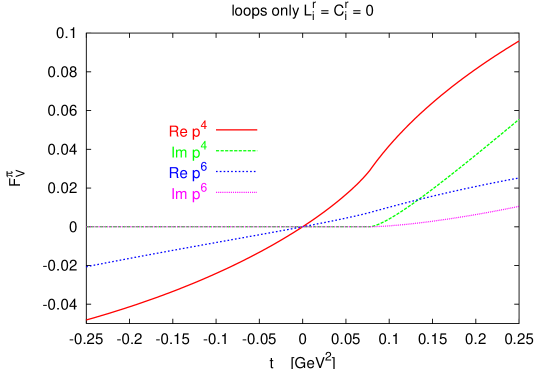
Figure 20: The real and imaginary parts of the loop diagrams at order $p^{6}$ and order $p^{6}$ with all $L_{i}^{r}=0$ and $C_{i}^{r}=0$, for the pion form-factor. Notice that there is convergence both for the real and the imaginary part. Figure from Ref. [123].

The calculation can now be used to fit to the available data. The fit is very similar to the one in the two-flavour case shown in Fig. 11. The data included in the best fit as shown in Fig. 21.

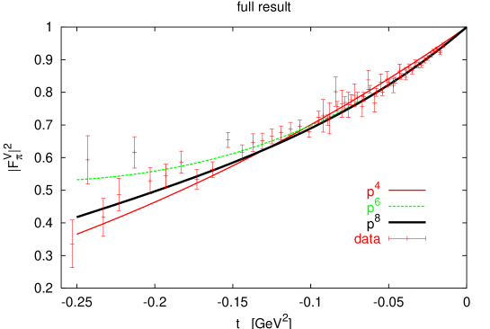
Figure 21: The comparison of the space-like measurements with the ChPT calculation for the pion electromagnetic form-factor. Notice that there is excellent convergence over the whole kinematical range. The curve labeled $p^{8}$ includes a term $c_{f}t^{3}$ in the fit in addition to the full order $p^{6}$ expression. The data are from Refs. [130, 131]. Figure from Ref. [123].

The inclusion of time-like data does not really change the fits as discussed in [73] and [123]. Figures for that part of the fits can be found in those references. Note there seems to be some numerical problems in the work of Ref. [127]. The real part of the result is compared with the measurements in the appendix of that reference but the imaginary part quoted there is much larger than thee one found in [123] and way too large to be compatible with the known pion phase-shift at that order in ChPT.

The fits of Ref. [123] allow to determine the parameter $L_{9}^{r}$ to order $p^{6}$ as

$$L_{9}^{r}(0.77~{}\mbox{GeV})=(5.93\pm 0.43)\times 10^{-3}\,.$$ (139)

The error due to experiment only is about half this, the remainder is mainly from the estimate of the order $p^{6}$ parameters that contributes proportional to $m_{\pi}^{2}$ or $m_{K}^{2}$. The curvature also has a contribution from an order $p^{6}$ constant allowing a direct determination giving [123].

$$R_{V2}^{\pi}=-4\left(C_{88}^{r}-C_{90}^{r}\right)=(0.22\pm 0.02)\times 10^{-3}\,.$$ (140)

This result is in good agreement with the various resonance estimates discussed below. Eqs. (139) and (140) are the direct three-flavour equivalents of the two-flavour results of Ref. [73] given in Eq. (3.6).

The kaon electromagnetic form-factors have also been calculated. The data here are not so good and there seem to be some problems with the absolute normalization. The data from Refs. [131, 132, 133] are in agreement with the results from ChPT within the experimental errors.

Electromagnetic form-factors are near $t=0$ often described by the charge radius defined by

$$\langle r^{2}\rangle_{V}^{\pi,K^{+},K^{0}}=6\left.\frac{d}{dt}F_{V}^{\pi,K^{+},K^{0}}\right|_{t=0}\,,$$ (141)

and the data and fits given can be used to extract/predict the various radii. This has been done in Refs. [73, 123] for the two- and three-flavour case respectively.

The $K^{0}$ electromagnetic radius has been measured in a kaon regeneration on electrons experiment [134] with the result

$$\langle r^{2}\rangle_{V}^{K^{0}}=(-0.054\pm 0.026)~{}\mbox{fm}^{2}\,.$$ (142)

The decay $K_{L}\to\pi^{+}\pi^{-}e^{+}e^{-}$ also has contributions that contain the neutral kaon electromagnetic form-factor but the extraction from the data is rather model dependent and I will not use these data. This radius was predicted in Refs. [126, 123], the result from [126] used older values of the order $p^{4}$ LECs. The prediction from [123] is

$$\langle r^{2}\rangle_{V}^{K^{0}} = \Big{\{}-0.0365[\mbox{loops }p^{4}]-0.0057[\mbox{loops }p^{6}]\Big{\}}~{}\mbox{fm}^{2}+\frac{6}{F_{\pi}^{4}}R_{V2}^{K^{0}}$$ (143)

$$= (-0.042\pm 0.012)~{}\mbox{fm}^{2}\,.$$

The error is based on assuming that the unknown contribution is not larger than twice the order $p^{6}$ loop contribution. The result is in good agreement with the measurement (142). We can also turn the argument around and obtain

$$R_{V2}^{K^{0}}=(-0.4\pm 0.9)\times 10^{-5}~{}{GeV}^{2}\,.$$ (144)

This result is in reasonable agreement with the resonance estimate presented in Ref. [123].

4.7 $K_{\ell 3}$

The decays considered in this subsection are

$$K^{+}(p) \rightarrow \pi^{0}(p^{\prime})\ell^{+}(p_{\ell})\nu_{\ell}(p_{\nu})\,,\hskip 28.45274pt[K_{\ell 3}^{+}]$$ (145)

$$K^{0}(p) \rightarrow \pi^{-}(p^{\prime})\ell^{+}(p_{\ell})\nu_{\ell}(p_{\nu})\,,\hskip 28.45274pt[K_{\ell 3}^{0}]$$ (146)

and their charge conjugate modes. $\ell$ stands for $\mu$ or $e$. The short notation for each decay is given in the square brackets.

The matrix-element for $K_{\ell 3}^{+}$, neglecting scalar and tensor contributions, has the structure

$$T = \frac{G_{F}}{\sqrt{2}}V_{us}^{\star}\ell^{\mu}{F_{\mu}}^{+}(p^{\prime},p)\,,$$ (147)

with

$$\ell^{\mu} = \bar{u}(p_{\nu})\gamma^{\mu}(1-\gamma_{5})v(p_{\ell})\,,$$

$${F_{\mu}}^{+}(p^{\prime},p) = <\pi^{0}(p^{\prime})\mid V_{\mu}^{4-i5}(0)\mid K^{+}(p)>\,,$$ (148)

$$= \frac{1}{\sqrt{2}}[(p^{\prime}+p)_{\mu}f^{K^{+}\pi^{0}}_{+}(t)+(p-p^{\prime})_{\mu}f_{-}^{K^{+}\pi^{0}}(t)].$$

To obtain the $K_{\ell 3}^{0}$ matrix-element, one replaces $F^{+}_{\mu}$ by

$${F_{\mu}}^{0}(p^{\prime},p) = <\pi^{-}(p^{\prime})\mid V_{\mu}^{4-i5}(0)\mid K^{0}(p)>$$ (149)

$$= (p^{\prime}+p)_{\mu}f^{K^{0}\pi^{-}}_{+}(t)+(p-p^{\prime})_{\mu}f_{-}^{K^{0}\pi^{-}}(t).$$

The processes (145) and (146) thus involve the four $K_{\ell 3}$ form-factors $f^{K^{+}\pi^{0}}_{\pm}(t)$, $f^{K^{0}\pi^{-}}_{\pm}(t)$ which depend on

$$t=(p^{\prime}-p)^{2}=(p_{\ell}+p_{\nu})^{2},$$ (150)

the square of the four momentum transfer to the leptons.

Only the isospin conserving part is known to order $p^{6}$. The isospin breaking corrections are one of the remaining unknowns in the determination of the CKM matrix-element $V_{us}$. In the isospin limit we have that

$$f_{\pm}=f_{\pm}^{K\pi}=f_{\pm}^{K^{+}\pi^{0}}=f_{\pm}^{K^{0}\pi^{-}}\,.$$ (151)

$f_{+}^{K\pi}$ is referred to as the vector form-factor, because it specifies the $P$-wave projection of the crossed channel matrix-elements $<0\mid V^{4-i5}_{\mu}(0)\mid K^{+},\pi^{0}\;\mbox{in}>$. The $S$-wave projection is described by the scalar form-factor

$$f_{0}(t)=f_{+}(t)+\frac{t}{m^{2}_{K}-m^{2}_{\pi}}f_{-}(t)\,.$$ (152)

Analyses of $K_{\ell 3}$ data frequently assume a linear dependence

$$f_{+,0}(t)=f_{+}(0)\left[1+\lambda_{+,0}\frac{t}{m^{2}_{\pi^{+}}}\right]\;\;.$$ (153)

For an early discussion of the validity of this approximation see [3] and references cited therein. As pointed out in Ref. [135] and checked afterwards by the ISTRA+ [136], KTeV [137] and NA48 [138], the linear approximation is not sufficient at the present level of precision.

The form-factors $f_{\pm,0}(t)$ are analytic functions in the complex $t$-plane cut along the positive real axis. The cut starts at $t=(m_{K}+m_{\pi})^{2}$. In the phase convention used here, the form-factors are real in the physical region

$$m^{2}_{\ell}\leq t\leq(m_{K}-m_{\pi})^{2}.$$ (154)

A discussion of the kinematics in $K_{\ell 3}$ decays can be found in [112] and references cited therein.

The total result can be split by chiral order

$$f_{i}(t)=f_{i}^{(2)}(t)+f_{i}^{(4)}(t)+f_{i}^{(6)}(t)\,,\quad(i=+,-,0)\,.$$ (155)

The lowest order result has been known for a very long time and is fully determined by gauge invariance.

$$f_{+}^{(2)}(t)=f_{0}^{(2)}(t)=1,,\quad\quad\quad f_{-}^{(2)}(t)=0\,.$$ (156)

The order $p^{4}$ contribution was first calculated within the ChPT framework by Gasser and Leutwyler [124] with earlier results by Leutwyler and Roos [139]. The result contains the nonanalytic dependence in the symmetry parameters predicted by [140]. Partial studies at order $p^{6}$ have also been done, the double logarithm contribution is small as was shown in Ref. [58] and a possibly large role for terms with two powers of quark masses has been argued for in Ref. [141]. The latter reference also pointed out the strong interdependence of the measurements of $F_{K}$ and $V_{us}$ as a possible solution to the CKM unitarity problem.

There exist two full calculations at order $p^{6}$. The work of Post and Schilcher [127] and Bijnens and Talavera [135]. The first work uses outdated values of the ChPT constants as well as an older version of the classification of $p^{6}$ constants. Due to the different methods of subtraction and splitting up the various proper two-loop integrals in an analytical and numerical part, a full analytical comparison between the two results has not been done. The parts which can be compared are in agreement analytically. The numerical results of both papers are in agreement for $f_{+}$ when the same input values for all parameters are used. There is a disagreement for $f_{-}$ but as discussed in Sect. 4.6 there are some indications for numerical errors in Ref. [127].

Let me now discuss the main results of Ref. [135]. I will present some of their numerical results later but first discuss the model-independent relations at order $p^{6}$. There are a large number of order $p^{6}$ LECs contributing to both form-factors, their contributions to the processes discussed in the previous, this one and the next subsection satisfy several relations. The combination which is relevant for the curvature of $f_{+}(t)$ is the same combination that appears in the curvature of the pion electromagnetic form-factor. Its value has been determined from the data and is given in Eq. (140). That way Ref. [135] predicted the curvature in $f_{+}(t)$. In a similar way, the curvature of the scalar form-factor, $f_{0}(t)$, is determined by the order $p^{6}$ constants $C_{12}^{r}$. Its value can in principle also be determined from the curvature of the pion scalar form-factor [142], Sect. 4.8 There are also relations between the order $p^{6}$ constants contributing to the various charge radii. This relation is essentially the Sirlin relation of [128, 129].

A more surprising relation that connects the values of $f_{+}(0)$ with the slope and curvature of the scalar form-factor $f_{0}(t)$, was discovered in Ref. [135]. One constructs the quantity

$$\tilde{f}_{0}(t)=f_{+}(t)+\frac{t}{m_{K}^{2}-m_{\pi}^{2}}\left(f_{-}(t)+1-F_{K}/F_{\pi}\right)=f_{0}(t)+\frac{t}{m_{K}^{2}-m_{\pi}^{2}}\left(1-F_{K}/F_{\pi}\right)\,.$$ (157)

This has no dependence on the $L_{i}^{r}$ at order $p^{4}$, only via order $p^{6}$ contributions. Inspection of the dependence on the $C_{i}^{r}$ shows that

$$\tilde{f}_{0}(t) = 1-\frac{8}{F_{\pi}^{4}}\left(C_{12}^{r}+C_{34}^{r}\right)\left(m_{K}^{2}-m_{\pi}^{2}\right)^{2}+8\frac{t}{F_{\pi}^{4}}\left(2C_{12}^{r}+C_{34}^{r}\right)\left(m_{K}^{2}+m_{\pi}^{2}\right)$$ (158)

$$-\frac{8}{F_{\pi}^{4}}t^{2}C_{12}^{r}+\overline{\Delta}(t)+\Delta(0)\,.$$

It should be emphasized that the quantities $\overline{\Delta}(t)$ and $\Delta(0)$ can in principle be calculated to order $p^{6}$ accuracy with knowledge of the $L_{i}^{r}$ to order $p^{4}$ accuracy. In practice, since a $p^{4}$ fit will include in the values of the $L_{i}^{r}$ effects that come from the $p^{6}$ loops (due to the fitting to experimental values) we consider the $p^{6}$ fits to be the relevant ones to avoid double counting effects.

The definition in (157) has essentially used the Dashen-Weinstein relation [143] to remove the $L_{i}^{r}$ dependence at order $p^{4}$. It has also the effect that it removed many of the $C_{i}^{r}$ from the scalar form-factor as well. The corrections which appear in the Dashen-Weinstein relation are include in the functions $\overline{\Delta}(t)$ and $\Delta(0)$, these have both order $p^{4}$ [124, 140] and order $p^{6}$ contributions.

It is obvious from Eq. (158) that the needed combination of $C_{i}^{r}$ can be determined from the slope and the curvature of the scalar form-factor in $K_{\ell 3}$ decays.

It seems possible that $C_{12}^{r}$ can be measured from the curvature of the pion scalar form-factor near 0 [142]. With this calculation is complete, one can use the dispersive estimates of the pion scalar form-factor together with only a $\lambda_{0}$ measurement in $K_{\mu 3}$ to obtain the $p^{6}$ value for $f_{+}(0)$. There are also some dispersive estimates for the relevant scalar form-factor. Unfortunately, these were not in a usable form [144] when Ref. [135] appeared, but have since been treated in Ref. [145]. Other estimates of the relevant constants are the one used in [135] coming from Ref. [139] and the resonance chiral theory result of [146].

One feature that is visible in Eq. 158 is that the value of $f_{+}(0)$ only differs from 1 by terms of order $(m_{K}^{2}-m_{\pi}^{2})^{2}$. This is not only true for the analytic contributions written out explicitly but also for the entire expressions for $f_{+}(0)$. This is known as the Ademollo-Gatto theorem [147] and holds to all orders in ChPT.

Let us now discuss the adequacy of the linear parameterization for the form-factors. In Ref. [135] it was pointed out the measured value of a form-factor at zero and the slope are rather dependent on the curvature, even if the data themselves do not show the presence of curvature. The fitted value of the slope and the form-factor at zero can change significantly outside the quoted errors due to this. This was shown in Ref. [135] for the case of the then best available data in both the neutral decay channel, CPLEAR [148] and charged decay channel, KEK-PS E246 [149]. This is shown in Fig. 22 for the KEK-PS E246 data. The discussion for the CPLEAR data can be found in Ref. [135].

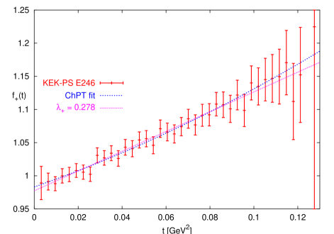
Figure 22: The KEK-PS E246 data together with the ChPT result, with the linear coefficient fitted and curvature predicted from ChPT as well as the linear fit of the KEK-PS collaboration.

The size of this effect is fairly small for the KEK-PS data but much larger for the CPLEAR data. It is very important to get data at small $t$ to minimize this effect as far as possible.

Since Ref. [135] appeared there have been newer high precisions data from the ISTRA+ [136], KTeV [137] and NA48 [138] collaborations. The last two have clearly demonstrated the existence of the curvature experimentally but there are some disagreements in their results. The question above is relevant now at a higher level of precision. How much does the presence of a $t^{3}$ term affect the latest high precision fits?

A recent reference discussing the various results and impact on the determination of $V_{us}$ is [146]. The final theoretical error has been significantly improved since the work of Leutwyler and Roos [139] and is now roughly one percent. The bulk of this comes from the uncertainty in the needed order $p^{6}$ constants. More theoretical work on dispersion relations in the scalar form-factor together with experimental studies of the scalar form-factor together with the relation discussed above should allow to pin down this contribution to better precision. The uncertainty on the theory side is definitely smaller than the violation of CKM unitarity when taking $V_{ud}$ from neutron beta decay.

4.8 Scalar form-factors

The scalar form-factors for the pions and kaons are defined as follows:

$$\langle M_{2}(p)|\bar{q}_{i}q_{j}|M_{1}(q)\rangle=F^{M_{1}M_{2}}_{ij}(t)$$ (159)

with $t=(p-q)^{2}$ and $i,j=u,d,s$. $M_{1}$, $M_{2}$ are meson states with the indicated momentum.

In the case of isospin symmetry $m_{u}=m_{d}=\hat{m}$, the various pion scalar form-factors obey

$$F_{S}^{\pi}(t) \equiv 2F^{\pi^{0}\pi^{0}}_{uu}(t)=2F^{\pi^{0}\pi^{0}}_{dd}(t)=2F^{\pi^{+}\pi^{+}}_{uu}(t)=2F^{\pi^{+}\pi^{+}}_{dd}(t)$$

$$= -2\sqrt{2}F^{\pi^{0}\pi^{+}}_{du}(t)=2\sqrt{2}F^{\pi^{0}\pi^{-}}_{ud}(t)\,,$$

$$F_{Ss}^{\pi} \equiv F^{\pi^{+}\pi^{+}}_{ss}=F^{\pi^{0}\pi^{0}}_{ss}\,.$$ (160)

The kaon currents are related by the rotations in flavour space

$$F_{Su}^{K}(t) \equiv F_{uu}^{K^{+}K^{+}(t)}=F_{dd}^{K^{0}K^{0}}(t)\,,$$

$$F_{Sd}^{K}(t) \equiv F_{dd}^{K^{+}K^{+}}(t)=F_{uu}^{K^{0}K^{0}}(t)\,,$$

$$F_{Ss}^{K}(t) \equiv F_{ss}^{K^{+}K^{+}}(t)=F_{ss}^{K^{0}K^{0}}(t)\,,$$

$$F_{S}^{K\pi}(t) \equiv F_{su}^{K^{0}\pi^{-}}(t)=\sqrt{2}F_{su}^{K^{+}\pi^{0}}(t)\,,$$

$$F_{Sq}^{K}(t) \equiv F_{Su}^{K}(t)+F_{Sd}^{K}(t)\,.$$ (161)

The other scalar form-factors can be obtained from the above using charge conjugation and time reversal. Eqs. (4.8) and (4.8) also show the notation used for the form-factors in the remainder of this subsection.

The scalar form-factor $F_{S}^{K\pi}(t)$ is proportional to the form-factor $f_{0}(t)$ used in $K_{\ell 3}$ decays, Sect. 4.7.

The scalar form-factors obey a relation similar to the Sirlin [128, 129] relation for the vector form-factor [142]

$$F_{S}^{\pi}(t)-2F_{Ss}^{\pi}(t)-2F_{Sd}^{K}(t)+2F_{Ss}^{K}(t)-4F_{S}^{K\pi}(t)=\mathcal{O}\left((m_{s}-\hat{m})^{2}\right)\,.$$ (162)

The proof of this relation is in App. A of Ref. [142] and uses a method similar to the one given in Ref. [129]. The data at present do not allow to test this result.

The values at zero momentum transfer are related to the derivatives of the masses w.r.t. to quark masses because of the Feynman-Hellman theorem (see [124])

$$F_{S}^{\pi}(0)=\frac{\partial}{\partial\hat{m}}m_{\pi}^{2}\,, F_{Ss}^{\pi}(0)=\frac{\partial}{\partial m_{s}}m_{\pi}^{2}\,,$$

$$F_{Su}^{K}(0)=\frac{\partial}{\partial m_{u}}m_{K}^{2}\,, F_{Ss}^{K}(0)=\frac{\partial}{\partial m_{s}}m_{K}^{2}\,,$$

$$F_{Sd}^{K}(0)=\frac{\partial}{\partial m_{d}}m_{K}^{2}\,.$$ (163)

The masses are known to order $p^{6}$ as discussed in Sect. 4.4 and there were sizable corrections at order $p^{6}$. This also shows that large corrections at $t=0$ can be expected. The argument goes as follows. If

$$m_{K}^{2}\approx B_{0}m_{s}+\beta(B_{0}m_{s})^{2}+\gamma(B_{0}m_{s})^{3}\,,$$ (164)

then

$$F_{Ss}^{K}(0)\approx B_{0}+2\beta B_{0}m_{s}+3\gamma(B_{0}m_{s})^{2}\,.$$ (165)

So we see that in the scalar form-factors the relative $p^{6}$ corrections can get enhanced by factors of order 3 compared to the masses.

The lowest order results have been long known. Order $p^{4}$ results were obtained in [124, 150]. The actual calculations of the scalar form-factor to order $p^{6}$ in three-flavour ChPT were performed by the authors of Ref. [142]. As expected from the argument just presented, large corrections were found to several of the form-factors involved, especially for the kaon ones. The results are also quite sensitive to the input values used for the LECs. In Fig. 23 the contributions to the two pion scalar form-factors at order $p^{4}$ and $p^{6}$ are shown. The are shown for the values of fit 10, one with a changed value for $L_{4}^{r}$ and the pure loop parts (all $L_{i}^{r}=0$). It is clear that while for these values the corrections are not enormous, they nonetheless are large and show no obvious convergence in that for many $t$ the order $p^{6}$ contribution is larger than order $p^{4}$.

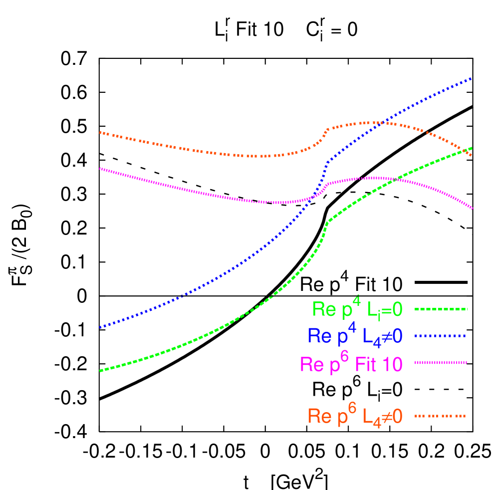
(a)

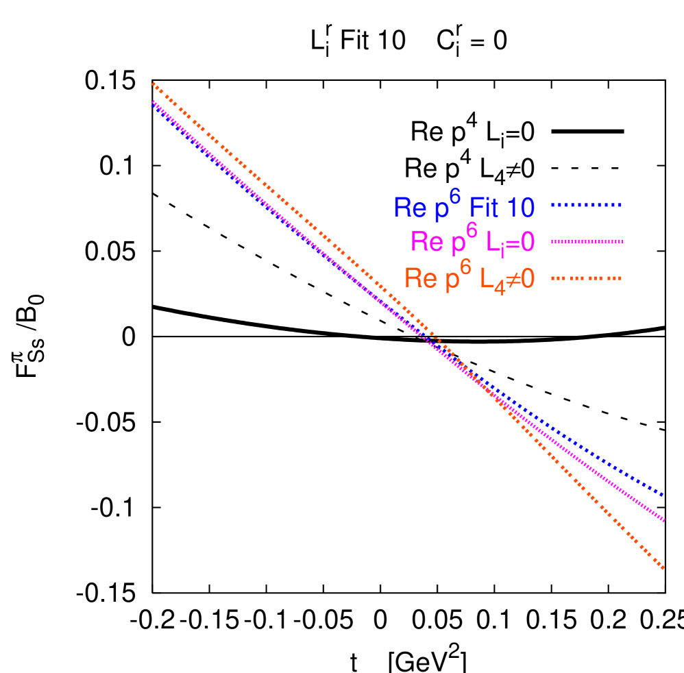
(b)

Figure 23: The effects of the $L_{i}^{r}$ on the various contributions to (a) $F^{\pi}_{S}(t)/(2B_{0})$ and (b) $F^{\pi}_{Ss}(t)/B_{0}$ as a function of $t$ for the case with $C_{i}^{r}=0$. The curves are for the real parts at order $p^{4}$ and order $p^{6}$. The curves labeled respectively Fit 10, $L_{4}^{r}\neq 0$ and $L_{i}^{r}=0$ are for the standard values of the $L_{i}^{r}$ of fit 10 in [107], the same values but $L_{4}^{r}=-0.003$ and with all $L_{i}^{r}=0$. Figure from Ref. [142].

The analysis for the pion and kaon form-factors followed the method introduced by Ref. [94] as updated in Refs. [105, 96]. The actual discussion of the results can be found in Ref. [142]. I will restrict myself to a few small comments here. One uses the ChPT input for the form-factors at zero and then calculates using the dispersive methods of Muskhelishvili-Omnès its momentum dependence. In order to have a consistent set of other LECs when $L_{4}^{r}$ and $L_{6}^{r}$ were varied, Ref. [142] redid the fits with the same assumptions as fit 10 in Ref. [107] but with range of inputs for those two $L_{i}^{r}$. The form-factors at zero momentum were then calculated from the order $p^{6}$ ChPT expression and the momentum dependence calculated from those with the dispersive method using [105, 96] result. The comparison of the dispersively estimated momentum dependence with the ChPT calculated momentum dependence leads to the constraint [142]

$$L_{6}^{r}\approx L_{4}^{r}-0.00035.$$ (166)

The comparison for the scalar radius is shown in Fig. 24. The constraint roughly describes the line where the ChPT and dispersive radius are in reasonable agreement.

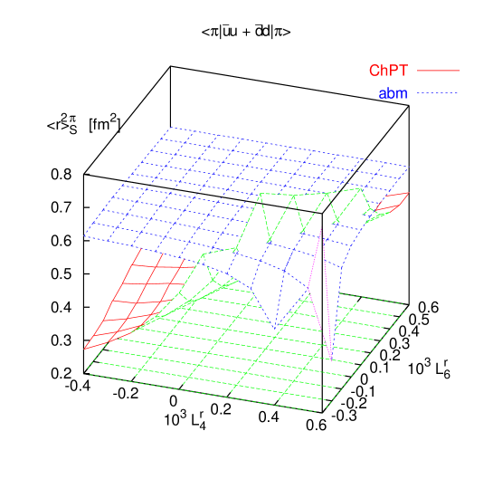
Figure 24: The result for the scalar radius $<r^{2}>_{\pi}^{S}$ as a function of $L_{4}^{r}$ and $L_{6}^{r}$, with the dispersive estimate (abm) and the ChPT calculation. Figure from Ref. [142].

That the actual values of $L_{4}^{r}$ and $L_{6}^{r}$ has a large impact on the masses and scalar sector is shown in Tab. 3.

Table 3: The results for various quantities for the $L_{i}^{r}$ of fit 10 and three other representative sets A, B and C. Adapted from Ref. [142].

Set	Fit 10	A	B	C
$10^{3}\cdot L_{4}^{r}$	0.0	0.4	0.5	0.5
$10^{3}\cdot L_{6}^{r}$	0.0	0.1	0.1	0.2
$F_{S}^{\pi}(0)/B_{0}$ (ChPT, $C_{i}^{r}=0$)	2.54	1.99	1.75	2.12
$F_{Ss}^{\pi}(0)/B_{0}$ (ChPT, $C_{i}^{r}=0$)	0.020	0.004	$-$0.002	0.008
$F_{Sq}^{K}(0)/B_{0}$ (ChPT, $C_{i}^{r}=0$)	1.94	1.36	1.12	1.51
$F_{Ss}^{K}(0)/B_{0}$ (ChPT, $C_{i}^{r}=0$)	1.77	1.35	1.17	1.45
$<r^{2}>^{\pi,disp}_{S}$ (fm2)	0.617	0.612	0.610	0.614
$<r^{2}>^{\pi,ChPT,C_{i}^{r}=0}_{S}$ (fm2)	0.384	0.547	0.625	0.563
$10^{5}\left(C_{12}^{r}+2C_{13}^{r}\right)\,[c_{S}^{\pi}]$	$-$2.6	$-$0.56	0.55	$-$0.71
$10^{5}\left(C_{12}^{r}+2C_{13}^{r}\right)[\gamma_{S}^{\pi}]$	$-$3.3	$-$0.55	0.48	$-$0.75
$10^{5}\left(C_{12}^{r}+2C_{13}^{r}\right)[\gamma_{Ss}^{K}]$	$-$0.55	0.11	0.33	0.15
$10^{5}\,C_{13}^{r}[\gamma_{Ss}^{\pi}]$	$-$0.56	$-$0.02	0.15	0.03
$10^{5}\left(C_{12}^{r}+4C_{13}^{r}\right)[\gamma_{Sq}^{K}]$	$-$4.1	$-$0.27	0.99	$-$0.08
$10^{5}\,C_{12}^{r}[c_{S}^{\pi},\,\gamma_{Ss}^{\pi}]$	$-$1.5	$-$0.52	0.26	$-$0.78
$10^{5}\,C_{12}^{r}[c_{S}^{\pi},\,\gamma_{Sq}^{K}]$	$-$1.1	$-$0.84	0.12	$-$1.3
$F_{0}$ (MeV)	87.7	63.5	70.4	71.0
$F_{\pi^{+}}^{(4)}$	0.136	0.230	0.253	0.254
$F_{\pi^{+}}^{(6)}$	$-$0.083	0.226	0.059	0.048
$F_{K\pi}^{(4)}$	0.169	0.157	0.153	0.159
$F_{K\pi}^{(6)}$	0.051	0.063	0.067	0.061
$\mu_{\pi}^{(2)}$	0.736	1.005	1.129	0.936
$\mu_{\pi}^{(4)}$	0.006	$-$0.090	$-$0.138	$-$0.043
$\mu_{\pi}^{(6)}$	0.258	0.085	0.009	0.107
$\mu_{K}^{(2)}$	0.687	0.938	1.055	0.874
$\mu_{K}^{(4)}$	0.007	$-$0.100	$-$0.149	$-$0.057
$\mu_{K}^{(6)}$	0.306	0.162	0.094	0.183
$\mu_{\eta}^{(2)}$	0.734	1.001	1.124	0.933
$\mu_{\eta}^{(4)}$	$-$0.052	$-$0.151	$-$0.197	$-$0.104
$\mu_{\eta}^{(6)}$	0.318	0.150	0.073	0.171

The masses and decay constants for the sets of input parameters given can also be found in Table 3. The various orders in the expansion quoted there are defined as:

$$F_{\pi^{+}}/F_{0} = 1+F_{\pi^{+}}^{(4)}+F_{\pi^{+}}^{(6)}\,,$$

$$F_{K^{+}}/F_{\pi^{+}} = 1+F_{K\pi}^{(4)}+F_{K\pi}^{(6)}\,,$$

$$m_{\pi^{\pm}}^{2}/(m_{\pi^{\pm}}^{2})_{\mbox{\tiny QCD}} = \mu_{\pi}^{(2)}+\mu_{\pi}^{(4)}+\mu_{\pi}^{(6)}$$

$$m_{K^{\pm}}^{2}/(m_{K^{\pm}}^{2})_{\mbox{\tiny QCD}} = \mu_{K}^{(2)}+\mu_{K}^{(4)}+\mu_{K}^{(6)}\,,$$

$$m_{\eta}^{2}/(m_{\eta}^{2})_{\mbox{\tiny phys}} = \mu_{\eta}^{(2)}+\mu_{\eta}^{(4)}+\mu_{\eta}^{(6)}\,.$$ (167)

Notice that in [107] the corresponding numbers were quoted for the “Main Fit” which used the old $K_{e4}$ data. In Ref. [142] several of the order $p^{6}$ constants were also determined from the curvature in the form-factors, these are the combinations of $C_{i}^{r}$ given in Tab. 3. The symbol in square brackets indicates the curvature of the form-factors used in the determination. The curvature is for the form-factor at zero normalized to 1, for the quantities labeled $c$. For the quantities labeled $\gamma$, the form-factors at zero are normalized to $B_{0}$ or to its lowest order value. It is obvious from the table that there are some discrepancies still to be understood since not all determinations are compatible. The table shows the very large corrections to some of the scalar form-factors at zero.

A glance at Table 3 shows that the pion decay constant in the chiral limit $F_{0}$ can be substantially different from the value of about $87~{}$MeV for the case of fit 10. The reason is that $L_{4}^{r}$ is not that well constrained and thus allows for these different values. As discussed in the two following subsections, the constraints from $\pi\pi$ scattering and $\pi K$ scattering could resolve this partly but the constraints are only marginally consistent. The consistent area does have values of $F_{0}$ very close to the one of fit 10. A full conclusion cannot be drawn as a comprehensive analysis of all order $p^{6}$ constants is still lacking.

4.9 Pion-pion scattering

We have already treated pion-pion scattering in two-flavour ChPT. In order to complete the check of going from $K_{\ell 4}$ form-factors to pion-pion scattering, the latter process also needs to be known to order $p^{6}$ in three-flavour ChPT. This was accomplished in Ref. [151]. All pion-pion scattering in the isospin limit can be described by the function $A(s,t,u)$ defined in Eq. (103).

This function was calculated in two-flavour ChPT to order $p^{6}$ in Refs. [72, 54] and is also known to order $p^{6}$ in three-flavour ChPT. The expression can be found in Ref. [151].

The convergence of the expansion is similar to the convergence in two-flavour ChPT. The various isospin amplitudes can be rewritten in terms of $A(s,t,u)$ via

$$T^{0}(s,t) = 3A(s,t,u)+A(t,u,s)+A(u,s,t)\,,$$

$$T^{1}(s,t) = A(t,u,s)-A(u,s,t)\,,$$

$$T^{2}(s,t) = A(t,u,s)+A(u,s,t)\,,$$ (168)

where the kinematical variables $t,u$ can be expressed in terms of $s$ and $\cos\theta$ as

$$t=-\frac{1}{2}(s-4m_{\pi}^{2})(1-\cos\theta)\,,\quad u=-\frac{1}{2}(s-4m_{\pi}^{2})(1+\cos\theta)\,.$$ (169)

The amplitudes are expanded in partial waves using

$$T^{I}(s,t)=32\pi\sum_{\ell=0}^{\infty}(2\ell+1)P_{\ell}(\cos\theta)t^{I}_{\ell}(s)\,.$$ (170)

Near threshold these can be expanded in terms of the threshold parameters

$$t^{I}_{\ell}=q^{2\ell}\left(a^{I}_{\ell}+b^{I}_{\ell}q^{2}+{\cal O}(q^{4})\right)\,,\quad q^{2}=\frac{1}{4}\left(s-4m_{\pi}^{2}\right)\,.$$ (171)

Below the inelastic threshold the partial waves satisfy

$$\mathrm{Im}t^{I}_{\ell}(s)=\sigma(s)\left|t^{I}_{\ell}(s)\right|^{2},\quad\quad\sigma(s)=\sqrt{1-\frac{4m_{\pi}^{2}}{s}}\,.$$ (172)

In this regime, all partial waves can be written in terms of the phase-shifts.

$$t^{I}_{\ell}(s)=\frac{1}{\sqrt{1-(4m_{\pi}^{2}/s)}}\,\frac{1}{2i}\left\{e^{2i\delta^{I}_{\ell}(s)}-1\right\}\,.$$ (173)

Some results of the phase-shifts were shown already for two-flavour QCD.

The three-flavour calculation results for the threshold parameters are shown in Tab. 4 for the sets of input parameters fit 10, A, B and C described in earlier subsections and in Tab. 3.

Table 4: The values of the threshold parameters defined in (171) for the values of the input parameters of fits 10 [107] and A,B,C [142]. The lowest order values and the contributions from the order $p^{6}$ LECs, $C_{i}^{r}$, are included. The threshold parameters are given in the corresponding power of $m_{\pi^{+}}^{2}$. Note that $a^{I}_{\ell}$ and $b^{I}_{\ell}$ are always given with the same power of ten. For fit 10, the three orders are quoted separately so the convergence can be judged. Table adapted from [151].

		fit 10			fit A	fit B	fit C
	$p^{2}$	$p^{4}$	$p^{6}$	total	total	total	total
$a^{0}_{0}$	0.159	0.044	0.016	0.219	0.220	0.220	0.221
$b^{0}_{0}$	0.182	0.073	0.025	0.279	0.282	0.282	0.282
$10\,a^{2}_{0}$	$-$0.454	0.030	0.013	$-$0.410	$-$0.427	$-$0.433	$-$0.428
$10\,b^{2}_{0}$	$-$0.908	0.151	0.025	$-$0.731	$-$0.755	$-$0.761	$-$0.760
$10\,a^{1}_{1}$	0.303	0.052	0.031	0.385	0.388	0.389	0.389
$10\,b^{1}_{1}$	$-$	0.029	0.038	0.067	0.064	0.063	0.063
$10^{2}\,a^{0}_{2}$	$-$	0.153	0.080	0.233	0.223	0.220	0.221
$10^{2}\,b^{0}_{2}$	$-$	$-$0.040	0.007	$-$0.033	$-$0.035	$-$0.036	$-$0.036
$10^{3}\,a^{2}_{2}$	$-$	0.327	$-$0.106	0.221	0.219	0.218	0.221
$10^{3}\,b^{2}_{2}$	$-$	$-$0.234	$-$0.151	$-$0.385	$-$0.386	$-$0.385	$-$0.387
$10^{4}\,a^{1}_{3}$	$-$	0.20	0.44	0.64	0.62	0.62	0.62
$10^{4}\,b^{1}_{3}$	$-$	$-$0.15	$-$0.20	$-$0.35	$-$0.34	$-$0.34	$-$0.34

It can already be seen from Tab. 4 that $a^{0}_{0}$ is very well predicted for sets of input parameters but $a^{2}_{0}$ is somewhat smaller than the result of Ref. [86]. Ref. [151] performed a full analysis, using the fits of [142] with the whole range of $L_{4}^{r},L_{6}^{r}$ as input to determine the best fits. It was found that $a_{0}^{0}$ always fitted nicely but that the value of $a_{0}^{2}$ restricted the values to a corner of the $L_{4}^{r},L_{6}^{r}$ only. In Fig. 25 the dispersive results from Ref. [86] are shown together with the three-flavour order $p^{6}$ ChPT results.

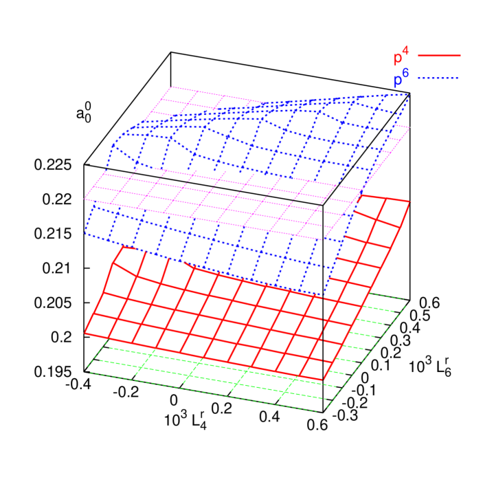
(a)

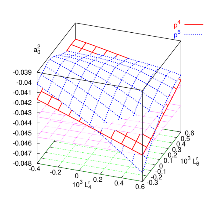
(b)

Figure 25: The scattering lengths $a^{0}_{0}$ and $a^{2}_{0}$ as a function of the input values $L_{4}^{r}$ and $L_{6}^{r}$ with the other $L_{i}^{r}$ simultaneously refitted to the $K_{e4}$ form-factors. (a) $a^{0}_{0}$ calculated to order $p^{4}$ and $p^{6}$. The central value of [86] of 0.220 is also shown. (b) $a^{2}_{0}$ at order $p^{4}$ and $p^{6}$. The two horizontal planes indicate the allowed region obtained in [86]. Figure from Ref. [151].

Similar results can be obtained for the other threshold parameters, but especially the higher threshold parameters have less convergence and have not been used as constraints. In Ref. [86, 151] one also defined the subtreshold parameters $C_{1}$ and $C_{2}$. They can similarly be used to obtain constraints on the ChPT input parameters. The total constraints from pion-pion scattering on the input parameters are shown in Fig. 26.

4.10 Pion-kaon scattering

An analysis of pion-kaon scattering similar to the combination of two-flavour ChPT at order $p^{6}$ and the Roy equations as done in Ref. [85, 86] can in principle also be done for pion-kaon scattering. At the moment, this is not quite completed. The Roy equations analysis, extended to the pion-kaon scattering case using the so-called Roy-Steiner equations has been performed by the authors of Ref. [152]. Some earlier sum rule work and comparisons with ChPT can be found in Ref. [153].

On the ChPT side, the lowest order calculation was performed using current algebra methods in Ref. [154]. The order $p^{4}$ calculation can be found in Refs. [155, 156] and the full order $p^{6}$ calculation was performed by the authors of Ref. [157].

An alternative method using ChPT, is to treat the kaon as very heavy and only the pion as a Goldstone boson. This so-called heavy-kaon approach to pion-kaon scattering can be found in Ref. [158].

The pion-kaon scattering system can be decomposed into different isospin amplitudes and these in turn can be expanded in partial waves. The partial wave in turn are expanded around threshold and a full set of threshold parameters can be defined analogous to the pion-pion scattering case. There also exist subtreshold expansions in the pion-kaon case as well. These quantities have been calculated using the Roy-Steiner equations in Ref. [152] and to order $p^{6}$ in three-flavour ChPT in Ref. [157].

The entire comparison of inputs to ChPT, the resulting threshold and subtreshold parameters and their comparison with the dispersive results can be done as in the previous subsection. The results for the threshold parameters and thee inputs of fit 10 are shown in Tab. 5.

Table 5: The results for the scattering lengths and ranges and the amplitude at the Cheng-Dashen point as well as the dispersive result. The scattering lengths and ranges are given in units of $m_{\pi^{+}}$. Table adapted from Ref. [157].

	Fit 10	[152]
$a^{1/2}_{0}$	0.220	$0.224\pm 0.022$
$10a^{1/2}_{1}$	0.18	$0.19\pm 0.01$
$10a^{3/2}_{0}$	$-0.47$	$-0.448\pm 0.077$
$10^{2}a^{3/2}_{1}$	0.31	$0.065\pm 0.044$
$10b^{1/2}_{0}$	1.3	$0.85\pm 0.04$
$10b^{3/2}_{0}$	$-0.27$	$-0.37\pm 0.03$
$T^{+}_{CD}$	2.11	$3.90\pm 1.50$

As can be seen, good agreement exists for many of the threshold parameters. A full analysis is described in Ref. [157] and the constraints on the $L_{4}^{r},L_{6}^{r}$ plane following are shown in Fig. 26.

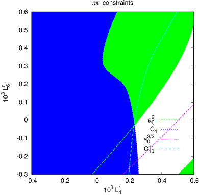
(a)

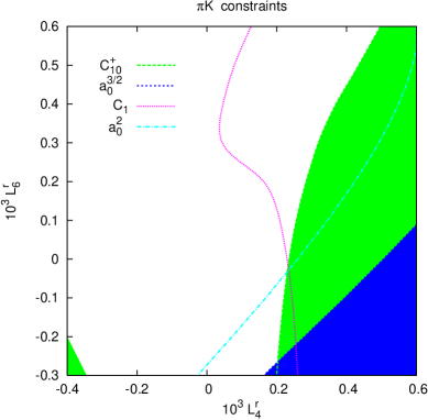
(b)

Figure 26: (a) The constraints on $L_{4}^{r}$ and $L_{6}^{r}$ following from the dispersive results in $\pi\pi$ scattering [85] as derived in [151]. (b) The same for the results from $\pi K$ scattering [152] as described in [157]. The curves from the boundaries are plotted on both plots to make comparisons easier. The shaded regions are excluded. Figure from Ref. [157].

A region that is compatible with all results is

$$L_{4}^{r}\approx 0.2\cdot 10^{-3}\quad\mbox{and}\quad L_{6}^{r}\approx 0.0\cdot 10^{-3}\,.$$ (174)

A more extensive discussion can be found in Ref. [157].

One point deserving mention, the order $p^{6}$ calculation naturally obeys the chiral relations derived in the heavy kaon approach [158]. In particular, how to obtain the isospin odd low-energy theorem from the full order $p^{6}$ expressions of [151] is discussed in Ref. [159]. There has also been some recent progress in calculating the threshold parameters fully analytically [160].

4.11 $\pi,K\to\ell\nu\gamma$

To determine the parameter $L_{10}^{r}$ at the same order as precision as was described in the previous subsections the processes $\pi,K\to\ell\nu\gamma$ need to be calculated to order $p^{6}$. This calculation has been done by the authors of Ref. [161]. They found a reasonably converging result. I refer to their paper for a longer discussion, but from Fig. 27 it can be seen that they found a nicely convergent series.

Figure 27: The axial vector form-factor in $\pi\to\ell\nu\gamma$ (left) and $K\to\ell\nu\gamma$ at order $p^{6}$ in ChPT. The dashed and solid curves represent the full results at order $p^{4}$ and order $p^{6}$. Note that the latter includes data fitting. Figure from Ref. [161].

4.12 Estimates of order $p^{6}$ constants

One of the major problems is the sheer number of order $p^{6}$ constants that contributes. In some cases, they could be determined from experiment directly. Good cases here are those responsible for kinematical quantities at order $p^{6}$. These are the constants responsible for the curvature in the various form-factors, the kinematic factors $b_{5}$ and $b_{6}$ in pion-pion scattering and similar quantities in other decays.

Especially the curvature in the vector form-factors leads to a well-determined combination. However, there are many more order $p^{6}$ LECs that cannot be so easily determined directly from data. Since at order $p^{6}$ typically many $L_{i}^{r}$ contribute to particular processes, the determination of them becomes entangled between different processes. As a result, an estimate of an order $p^{6}$ LEC used in one process where an $L_{i}^{r}$ is determined sneaks in the determination of the other $L_{i}^{r}$ and possibly order $p^{6}$ constants in the other processes.

The solution, a full comprehensive analysis of all processes at the same time is a major undertaking which has not been done. It is also not clear whether sufficient data exist to constrain all involved $L_{i}^{r}$ and order $p^{6}$ LECs.

The solution which has mainly been used up to the present is to estimate the values of the order $p^{6}$ LECs by simple resonance saturation. This approach was started already in Ref. [2]. There it was shown that the experimental values of the order $p^{4}$ LECs cannot be the low-energy limit of the linear sigma model. They also found that exchange of vector mesons lead to reasonable predictions for the largest LECs at order $p^{4}$. This work was systematized in Refs. [162] where it was shown that the values of all order $p^{4}$ constants can be understood on the basis of one-resonance exchange. Ref. [163] showed how these results, when taken together with short-distance QCD constraints, are independent of the actual chiral representation chosen for the resonance fields. They also found that the main contribution came from the exchange of vector mesons.

The approach used in most order $p^{6}$ papers consists in taking the simplest Lagrangian containing vector, axial-vector, scalar and sometimes pseudoscalar and tensor resonances, fitting its parameters as much as possible from data, and then taking the masses large to determine the LECs of ChPT. This is what has been done in basically all of the papers reviewed so far, with the exception of the two-flavour pion-pion scattering work.

The main underlying theory argument is the large number of colours, $N_{c}$, limit [164], where QCD reduces to a theory of stable resonances. The additional assumption made in the estimates is that the lowest resonance in each channel will be important.

Apart from the simplest version mainly used in the papers on ChPT to order $p^{6}$ more comprehensive approaches exist. There is the minimal hadronic approximation approach [165], the ladder resummation model approach [166] and the resonance chiral model approach [167, 146, 168, 169]. All of these approaches are different ways of taking a certain number of resonances into account in each channel. They differ somewhat in the way the various couplings are treated. One problem is that there is an ambiguity in how one deals with short distance QCD constraints. It is known that there are incompatibilities for a finite number of resonances [166].

Other approaches are the older quark model approach, see [170] and references therein, as well those based on the Nambu-Jona-Lasinio model [171], see [172, 173, 174, 175] and references therein. All these approaches give similar results in vector dominated channels but in those cases where quark mass effects play a major role, no full comparison with experimentally determined higher order coefficients has been done. For predictions regarding order $p^{4}$ LECs, most of these get similar results.

One problem that affects all the large $N_{c}$ based methods is that the ChPT LECs are subtraction scale dependent while the estimates are not. This can only be solved by going beyond the leading terms in $1/N_{c}$ also in the resonance models. Some attempts where also more references can be found are in Refs. [176, 177, 178].

This area of estimating higher order $p^{6}$ LECs is where most improvement is needed in the future of higher order ChPT calculations.

5 Other

In this section I dicuss the order $p^{6}$ calculations which have been done but which did not fit in the two main parts discussed in the previous two sections.

5.1 Finite temperature and volume calculations

The field of finite temperature calculations was started by Gasser and Leutwyler in Ref [179]. It means making the time part periodic and rotating it into the imaginary time direction. Two-loop calculations I am aware of in this area are the density dependence of the pion propagator by Schenk [180], as well as the pion mass and decay constant by Toublan [181].

At finite volume, there exists also work. Finite volume in ChPT was introduced by Gasser and Leutwyler in Ref. [182]. A lot of work has been done to higher orders in this area using Lüscher’s method to determine the leading finite volume correction [183]. Proper two-loop calculations at finite volume in ChPT have only become available recently. The mass and the decay constant in two-flavour ChPT can be found in Ref. [184] and the quark-antiquark condensate in three-flavour ChPT in Ref. [185].

There is another regime at finite volume, the small volume or $\epsilon$ regime. Here the lowest mode of zero momentum dominates the higher order corrections. It therefore needs to taken into account exactly and forms in this way a all-order calculation. This is a large area of active research and I will not discuss it here.

5.2 Partially quenched calculations

A large effort goes into numerically evaluating the functional integral of QCD. This is area is known as lattice QCD. One of the things that appears naturally in the way those calculations are done is the different treatment of quark lines connected to external legs, so-called valence quark lines, and the closed quark loops, called sea-quark loops.

The effect of the latter is numerically very difficult to compute and has therefore often been approximated. Neglecting the sea-quarks completely is known as the quenched approximation and treating them with different masses from the valence quarks is known as the partially quenched approximation.

In neither of these cases is the resulting theory a bona-fide field theory and the arguments that derive ChPT from QCD, given clearly in Ref. [40] do not all hold. But both quenched and partially-quenched are still well defined statistical models and many of the arguments when thought of in terms of Feynman diagrams still seem to hold. We can thus hope that a ChPT extended to the case of quenched and partially quenched QCD still makes sense. Many of the qualitative prediction predicted by quenched ChPT (QChPT) and partially quenched ChPT (PQChPT) seem to be present in actual lattice QCD calculations. Especially the quenched chiral logarithms seem to exist.

The extension of ChPT to the quenched case was started by Morel [186] and properly extended by Sharpe [187, 188] and Bernard and Golterman [189]. Infinities and Lagrangians at one-loop have been discussed in Ref. [190]. The extension to the partially quenched case was again done by Bernard, Golterman and Sharpe [191, 192]. Articles which provide a good overview of the field at order $p^{4}$ are Refs. [193, 194].

Work on extending the work to two-loops started some years ago but there were two difficulties to be solved. One is to find the checks coming from the knowledge of the divergence structure and the Lagrangian at order $p^{6}$ and the other is the sheer complexity of the calculations in terms of the size of the expressions. The solution to the former turned out to be easy. Already in Ref. [190] it was noted that the quenched Lagrangian and infinity structure at order $p^{4}$ had a very strong resemblance to the one of $n_{F}$-flavour ChPT at the same order. More arguments for this were given in Ref. [195]. When Bijnens, Danielsson and Lähde started looking at two-loop PQChPT, they realized that a very simple recipe allowed to obtain the full order $p^{6}$ both for the Lagrangian and the divergence structure. To understand this, one goes back to the suggestion of Morel [186] how to deal with the quenched approximation systematically. This is the approach worked out properly by Ref. [189]. In order to systematically remove the closed quark loops, one adds for each quark a bosonic quark, spin 1/2 but bosonic. Due to the different statistics, in this way all closed loops are exactly canceled. Partially quenched can be treated by leaving some of the quarks without a bosonic partner. Closed loops from these quarks then are not canceled. The formalism used in ChPT can be fully extended to this case by using supertraces instead of traces and adding extra bosonic and fermionic “Goldstone bosons.” It was then also shown that in the partially quenched case the equivalent of the singlet eta would be heavy and could be systematically removed from the theory [194]. With that in hand, one realizes that all manipulations done in $n_{F}$-flavour ChPT to obtain Lagrangians and divergence structures go through with the changes mentioned above and $n_{F}$ changed to the number of active sea-quarks. The PQChPT Lagrangian at order $p^{6}$ and the divergence structure can thus be derived immediately from the work of Refs. [51, 53]. One also sees immediately the origin of the extra order $p^{4}$ term of [196]. The number of terms in the Lagrangian this leads to is given in Tab. 2.

The complexity of the calculations was solved by combining the power of FORM [197] with a large amount of hand-optimized simplification of the various terms. At present no direct comparison with data are made, so I only show a representative plot. The relative corrections to lowest order for the case with three sea-quark flavours and valence-quarks of equal quark-mass, $m_{4}$, and sea-quarks of equal quark-mass, $m_{2}$, are shown in Fig. 28. Some visible features are the sizable corrections and the fact that the corrections do not vanish when $m_{1}\to 0$ but $m_{4}$ kept fixed. The latter is the manifestation of the quenched chiral logarithm. More details can be found in the actual papers [198, 199, 200, 201].

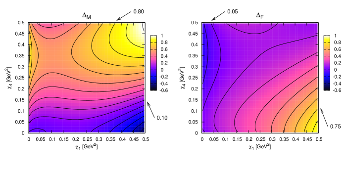
Figure 28: The relative corrections to the charged pseudoscalar meson mass, $\Delta_{M}$, and decay constant, $\Delta_{F}$, to NNLO for the case of three sea-quarks. The valence quarks have quark-mass $m_{1}$ and the sea-quarks mass $m_{4}$. The plot is as a function of the quark-masses in the combination $\chi_{1}=2B_{0}m_{1}$ and $\chi_{4}=2B_{0}m_{4}$. The quantity plotted represents the sum of the NLO and NNLO corrections normalized to lowest order. The difference between two successive contour lines in the plots is $0.10$. The values chosen for the LECs correspond to ”fit 10” of Ref. [107]. Figure from Ref. [201].

The actual calculations that have been performed are the masses for three sea-quarks [198, 201], the decay constants for three sea-quarks [199, 201] and the same quantities for two sea-quark flavours as well [200]. The expressions can be found on the website [19].

This is clearly an area where further progress is desirable.

6 Conclusions

In this review I have briefly discussed the foundations of ChPT and some of its technical aspects. The longest parts has been concerned with the actual calculations which have been performed at order $p^{6}$ and their confrontation with experimental results.

Here the two-flavour part, Sect. 3, is in rather good shape. Most calculations have been done and in many cases the contributions from unknown order $p^{6}$ constants are expected to be rather small. I particularly want to emphasize again here the work on pion-pion scattering where major progress in the theoretical description was made.

In the three-flavour sector, Sect. 4, many calculations have been done and fitted to experimental results. One main highlight here is the predictions made in the context of $K_{\ell 3}$ and its relation to the determination of $V_{us}$ but many other low-energy processes involving kaons and etas are also known. I have only briefly discussed the main remaining block towards a full comprehensive application of ChPT at NNLO, estimating in a consistent fashion all needed order $p^{6}$ LECs. Work in this area is going on, so I hope there will be significant progress in the not-too-distant future.

And last, I have mentioned the finite temperature, volume and partially quenched work to two-loop order in ChPT. The interface between lattice QCD and ChPT is a growing area of research and should benefit both communities. At present only a few full two-loop order calculations in this sector are available as discussed in Sect. 5.

Appendix A A few remarks on alternative notations

I have tried to stick in this review to one choice of notation. Many alternative parameterizations have been around especially for the two-flavour case.

There are two main conventions around for the parameters $\hat{F},F_{0},F$ which differ by a factor of $\sqrt{2}$. Which is in use can normally be detected by the forefactor in Eq. (48). $F^{2}/4$ corresponds to an $F_{\pi}$ of order 93 MeV, $F^{2}/8$ to an $F_{\pi}$ of order 130 MeV while in the older literature sometimes even an $F_{\pi}$ of order 180 MeV appears.

The parameters $\hat{B},B_{0},B$ often appear in the combination $\hat{F}^{2}\hat{B}/2$ which is frequently called $r$.

Many people use a left-right version instead of the right-left version introduced in Ref. [3]. They typically use $\Sigma=U^{\dagger}$ as the quantity containing the Goldstone bosons. The quantity $u$ also appears often denoted as $\xi$ and exists as well in a version with left and right interchanged.

For the two-flavour case, the fact that

$$SU(2)\times SU(2)/Z_{2}=SO(4)$$ (175)

and

$$SU(2)/Z_{2}=SO(3)\,,$$ (176)

allows a parameterization inspired by the breaking of $SO(4)$ to $SO(3)$. These are sometimes called sigma-model parameterizations. In Ref. [2] a four-vector $U=(U^{0},U^{1},U^{2},U^{3})$ was used with the restriction $U^{T}U=1$. Here the pion fields appear via $U^{i}=\pi^{i}/F$ for $i=1,2,3$. All needed external fields can also be brought into this representation. The explicit connection between the exponential and the sigma-model representation is

$$U^{i}=-\frac{i}{2}\langle\tau^{i}U\rangle$$ (177)

where the $\tau^{i}$ are the three Pauli-matrices. Weinberg often uses a three-vector $\vec{\pi}$, and a covariant derivative which depends nonlinearly on the $\vec{\pi}$ field. This is the form he used in his original paper [37].

All of these parameterizations are equivalent, as it has been proven that all can be brought into one standard form in Ref. [38]. However, when performing calculations, individual Feynman diagrams can be quite different in the different formulations. As an example, the pion wave function renormalization vanishes at NLO in the parameterization of Ref. [2] but it doesn’t in the exponential parameterization used in this paper.

References

- [1] S. Weinberg, Physica A 96 (1979) 327.
- [2] J. Gasser and H. Leutwyler, Annals Phys. 158 (1984) 142.
- [3] J. Gasser and H. Leutwyler, Nucl. Phys. B 250 (1985) 465.
- [4] A. Pich, Lectures at Les Houches Summer School in Theoretical Physics, Session 68: Probing the Standard Model of Particle Interactions, Les Houches, France, 28 Jul - 5 Sep 1997, [hep-ph/9806303].
- [5] S. Scherer, Adv. Nucl. Phys., 27 (2002) 277 [hep-ph/0210398].
- [6] S. Scherer and M. R. Schindler, preprint hep-ph/0505265.
- [7] G. Ecker, Lectures given at Advanced School on Quantum Chromodynamics (QCD 2000), Benasque, Huesca, Spain, 3-6 Jul 2000, preprint hep-ph/0011026.
- [8] J. Gasser, Lectures given at 41st Internationale Universitaetswochen fuer Theoretische Physik (International University School of Theoretical Physics): Flavor Physics (IUTP 41), Schladming, Styria, Austria, 22-28 Feb 2003. Lect. Notes Phys. 629 (2004) 1 [hep-ph/0312367].
-
[9]
H. Leutwyler,
Contribution to the Festschrift in honor of B.L. Ioffe,
At the frontier of particle physics,
Shifman, M. (ed.), vol. 1 pages 271-316.
preprint hep-ph/0008124;
H. Leutwyler, preprint hep-ph/9406283, lectures given at the Hadrons 94 Workshop, Gramado, Brazil, 10-14 Apr 1994. - [10] J. Donoghue, E. Golowich and B. Holstein, “Dynamics of the Standard Model,” Cambridge University Press, Cambridge, UK (1992).
- [11] H. Georgi, “Weak interactions and modern particle theory,” Benjamin/Cummings, Menlo Park CA, USA (1984).
- [12] A. Smilga, “Lectures on quantum chromodynamics,” World Scientific, Singapore (2001).
- [13] G. Ecker, Prog. Part. Nucl. Phys. 35 (1995) 1 [hep-ph/9501357].
- [14] U. G. Meissner, Rept. Prog. Phys. 56 (1993) 903 [hep-ph/9302247].
- [15] B. Ananthanarayan and B. Moussallam, JHEP 0406 (2004) 047 [hep-ph/0405206].
- [16] J. Gasser, A. Rusetsky and I. Scimemi, Eur. Phys. J. C32 (2003) 97 [hep-ph/0305260].
-
[17]
J. Gasser, M. A. Ivanov, E. Lipartia, M. Mojzis and A. Rusetsky,
Eur. Phys. J. C26 )2002) 13
[hep-ph/0206068],
V. Antonelli, A. Gall, J. Gasser and A. Rusetsky, Annals Phys. 286 (2001) 108 [hep-ph/0003118],
J. Gasser, V. E. Lyubovitskij, A. Rusetsky and A. Gall, Phys. Rev. D64 (2001) 016008 [hep-ph/0103157]. - [18] S. R. Beane, P. F. Bedaque, W. C. Haxton, D. R. Phillips and M. J. Savage, nucl-th/0008064.
- [19] The links can be found on the website http://www.thep.lu.se/bijnens/chpt.html.
- [20] J. Bijnens, Int. J. Mod. Phys. A 8 (1993) 3045.
- [21] J. Bijnens, L. Girlanda and P. Talavera, Eur. Phys. J. C 23 (2002) 539 [hep-ph/0110400].
- [22] T. Ebertshauser, H. W. Fearing and S. Scherer, Phys. Rev. D 65 (2002) 054033 [hep-ph/0110261].
- [23] S. L. Adler Phys. Rev.177 (1969) 2426; J. S. Bell and R. Jackiw, Nuovo Cim.A60 (1969) 47
- [24] G. ’t Hooft Phys. Rev. D14 (1976) 3432 [Erratum-ibid. D18 (1978) 2199]
- [25] M. Peskin and D. Schroeder, “An Introduction to quantum field theory,” Perseus Books, Reading MA, USA (1995).
- [26] J. Wess and B. Zumino, Phys. Lett. B 37 (1971) 95.
- [27] E. Witten, Nucl. Phys. B 223 (1983) 422.
-
[28]
J. Goldstone,
Nuovo Cim. 19 (1961) 154;
J. Goldstone, A. Salam and S. Weinberg, Phys. Rev. 127 (1962) 965. - [29] Y. Nambu, Phys. Rev. Lett. 4 (1960) 380; Phys. Rev. 117 (1960) 648.
- [30] C. P. Burgess Phys. Rept. 330 (2000) 193 [hep-th/9808176].
- [31] S. R. Coleman and E. Witten, Phys. Rev. Lett. 45 (1980) 100.
- [32] C. Vafa and E. Witten, Phys. Rev. Lett. 53 (1984) 535; Nucl. Phys. B 234 (1984) 173.
- [33] G. ’t Hooft, Naturalness, chiral symmetry, and spontaneous chiral symmetry breaking, lecture given at Cargese Summer Inst., Cargese, France, Aug 26 - Sep 8, 1979, in Recent developments in gauge theories : proceedings G. ’t Hooft, C. Itzykson, A. Jaffe, H. Lehmann, P.K. Mitter, I.M. Singer, R. Stora (eds), NATO Advanced Study Institute, Series B: Physics, v. 59, Plenum Press, 1980. Reprinted in ’t Hooft, G. (ed.): Under the spell of the gauge principle, p. 352-374.
- [34] M. L. Goldberger and S. B. Treiman, Phys. Rev. 110 (1958) 1178.
- [35] G. Colangelo, J. Gasser and H. Leutwyler, Phys. Rev. Lett. 86, 5008 (2001) [hep-ph/0103063].
- [36] S. Descotes-Genon, L. Girlanda and J. Stern, Eur. Phys. J. C 27 (2003) 115 [hep-ph/0207337].
- [37] S. Weinberg, Phys. Rev. 166 (1968) 1568.
- [38] S. R. Coleman, J. Wess and B. Zumino Phys. Rev. 177 (1969) 2239.
- [39] C. G. Callan, S. R. Coleman, J. Wess and B. Zumino Phys. Rev. 177 (1969) 2247.
- [40] H. Leutwyler, Annals Phys. 235 (1994) 165 [hep-ph/9311274].
- [41] J. Stern, H. Sazdjian and N. H. Fuchs, Phys. Rev. D 47 (1993) 3814 [hep-ph/9301244].
- [42] S. Weinberg, Phys. Rev. Lett. 17 (1966) 616.
- [43] C. Itzykson and J. Zuber, “Quantum Field Theory.” McGraw-Hill, New York, USA (1980).
- [44] E. D’Hoker and S. Weinberg, Phys. Rev. D 50 (1994) 6050 [hep-ph/9409402].
-
[45]
G. ’t Hooft and M. J. G. Veltman,
Nucl. Phys. B 44 (1972) 189;
C. G. Bollini and J. J. Giambiagi, Phys. Lett. B 40 (1972) 566. -
[46]
J. Bijnens and B. Guberina,
Phys. Lett. B 205 (1988) 103;
I.S. Gerstein et al., Phys. Rev. D 3 ( 1971 ) 2486;
A.C. Redfield, Phys. Lett. B 109 (1982) 311;
J. Honerkamp and K. Meetz, Phys. Rev. D 3 ( 1971 ) 1996;
J.M. Charap, Phys. Rev. D 3 (1971) 1998. - [47] J.C. Collins, “Renormalization,” Cambridge University Press, Cambridge, 1984.
- [48] J. F. Donoghue and D. Wyler, Nucl. Phys. B 316 (1989) 289.
- [49] J. Bijnens, A. Bramon and F. Cornet, Z. Phys. C 46 (1990) 599.
- [50] H. W. Fearing and S. Scherer, Phys. Rev. D 53 (1996) 315 [hep-ph/9408346].
- [51] J. Bijnens, G. Colangelo and G. Ecker, J. High Energy Phys. 9902 (1999) 020 [hep-ph/9902437].
- [52] S. Scherer and H. W. Fearing, Phys. Rev. D 52 (1995) 6445 [hep-ph/9408298].
- [53] J. Bijnens, G. Colangelo and G. Ecker, Annals Phys. 280 (2000) 100 [hep-ph/9907333].
- [54] J. Bijnens, G. Colangelo, G. Ecker, J. Gasser and M. E. Sainio, Nucl. Phys. B 508 (1997) 263 [Erratum-ibid. B 517 (1998) 639] [hep-ph/9707291].
- [55] W. A. Bardeen, A. J. Buras, D. W. Duke and T. Muta, Phys. Rev. D 18 (1978) 3998.
- [56] I. Jack and H. Osborn, Nucl. Phys. B 207, 474 (1982).
- [57] G. Colangelo, Phys. Lett. B 350, 85 (1995) [Erratum-ibid. B 361, 234 (1995)] [hep-ph/9502285].
- [58] J. Bijnens, G. Colangelo and G. Ecker, Phys. Lett. B 441 (1998) 437 [hep-ph/9808421].
- [59] M. Buchler and G. Colangelo, Eur. Phys. J. C 32 (2003) 427 [hep-ph/0309049].
- [60] J. Gasser and U. G. Meissner, Nucl. Phys. B 357 (1991) 90.
- [61] M. Knecht, B. Moussallam, J. Stern and N. H. Fuchs, Nucl. Phys. B 457 (1995) 513 [hep-ph/9507319].
- [62] G. Colangelo, M. Finkemeier and R. Urech, Phys. Rev. D 54, 4403 (1996) [hep-ph/9604279].
- [63] J. Bijnens and F. Cornet, Nucl. Phys. B 296 (1988) 557.
- [64] J. F. Donoghue, B. R. Holstein and Y. C. Lin, Phys. Rev. D 37 (1988) 2423.
- [65] H. Marsiske et al. [Crystal Ball Collaboration], Phys. Rev. D 41 (1990) 3324.
- [66] D. Morgan and M. R. Pennington, Phys. Lett. B 272 (1991) 134.
- [67] S. Bellucci, J. Gasser and M. E. Sainio, Nucl. Phys. B 423, 80 (1994) [Erratum-ibid. B 431, 413 (1994)] [hep-ph/9401206].
- [68] J. Gasser and M. E. Sainio, Eur. Phys. J. C 6 (1999) 297 [hep-ph/9803251].
- [69] J. Gasser, M. A. Ivanov and M. E. Sainio, Nucl. Phys. B 728 (2005) 31 [hep-ph/0506265].
- [70] U. Burgi, Phys. Lett. B 377, 147 (1996) [hep-ph/9602421].
- [71] U. Burgi, Nucl. Phys. B 479 (1996) 392 [hep-ph/9602429].
- [72] J. Bijnens, G. Colangelo, G. Ecker, J. Gasser and M. E. Sainio, Phys. Lett. B 374 (1996) 210 [hep-ph/9511397].
- [73] J. Bijnens, G. Colangelo and P. Talavera, J. High Energy Phys. 9805 (1998) 014 [hep-ph/9805389].
- [74] J. F. Donoghue and B. R. Holstein, Phys. Rev. D 48 (1993) 137 [hep-ph/9302203].
- [75] L. V. Fil’kov and V. L. Kashevarov, Phys. Rev. C 72 (2005) 035211 [nucl-th/0505058].
- [76] J. Ahrens et al., Eur. Phys. J. A 23 (2005) 113 [nucl-ex/0407011].
- [77] L. V. Fil’kov and V. L. Kashevarov, preprint nucl-th/0512047.
- [78] J. Gasser, M. A. Ivanov and M. E. Sainio, preprint hep-ph/0602234.
- [79] J. Boyer et al., Phys. Rev. D 42 (1990) 1350.
- [80] J. Gasser and H. Leutwyler, Phys. Lett. B 125 (1983) 325.
- [81] L. Rosselet et al., Phys. Rev. D 15, 574 (1977).
- [82] S. M. Roy, Phys. Lett. B 36, 353 (1971).
- [83] B. Ananthanarayan, G. Colangelo, J. Gasser and H. Leutwyler, Phys. Rept. 353 (2001) 207 [hep-ph/0005297].
- [84] S. Descotes-Genon, N. H. Fuchs, L. Girlanda and J. Stern, Eur. Phys. J. C 24 (2002) 469 [hep-ph/0112088].
- [85] G. Colangelo, J. Gasser and H. Leutwyler, Phys. Lett. B 488 (2000) 261 [hep-ph/0007112].
- [86] G. Colangelo, J. Gasser and H. Leutwyler, Nucl. Phys. B 603 (2001) 125 [hep-ph/0103088].
- [87] S. Pislak et al. [BNL-E865 Collaboration], Phys. Rev. Lett. 87 (2001) 221801 [hep-ex/0106071].
- [88] S. Pislak et al. [BNL-E865 Collaboration], Phys. Rev. D 67 (2003) 072004 [hep-ex/0301040].
- [89] B. Adeva et al. [DIRAC Collaboration], Phys. Lett. B 619 (2005) 50 [hep-ex/0504044].
- [90] J. R. Pelaez and F. J. Yndurain, Phys. Rev. D 68, 074005 (2003) [hep-ph/0304067].
- [91] J. R. Pelaez and F. J. Yndurain, Phys. Rev. D 71, 074016 (2005) [hep-ph/0411334].
- [92] I. Caprini, G. Colangelo, J. Gasser and H. Leutwyler, Phys. Rev. D 68, 074006 (2003) [hep-ph/0306122].
- [93] I. Caprini, G. Colangelo and H. Leutwyler, Int. J. Mod. Phys. A 21 (2006) 954 [hep-ph/0509266].
- [94] J. F. Donoghue, J. Gasser and H. Leutwyler, Nucl. Phys. B 343 (1990) 341.
- [95] B. Moussallam, Eur. Phys. J. C 14 (2000) 111 [hep-ph/9909292].
- [96] B. Ananthanarayan, P. Buttiker and B. Moussallam, Eur. Phys. J. C 22 (2001) 133 [hep-ph/0106230].
- [97] B. Ananthanarayan, I. Caprini, G. Colangelo, J. Gasser and H. Leutwyler, Phys. Lett. B 602 (2004) 218 [hep-ph/0409222].
- [98] J. Bijnens and P. Talavera, Nucl. Phys. B 489, 387 (1997) [hep-ph/9610269].
-
[99]
S. M. Korenchenko [PIBETA Collaboration],
Phys. Atom. Nucl. 68 (2005) 498
[Yad. Fiz. 68 (2005) 527];
D. Pocanic [PIBETA Collaboration], Int. J. Mod. Phys. A 20 (2005) 472 [hep-ph/0407198]. - [100] E. Golowich and J. Kambor, Nucl. Phys. B 447, 373 (1995) [hep-ph/9501318].
- [101] G. Amoros, J. Bijnens and P. Talavera, Nucl. Phys. B 568 (2000) 319 [hep-ph/9907264].
- [102] S. Dürr and J. Kambor, Phys. Rev. D 61 (2000) 114025 [hep-ph/9907539].
- [103] K. Maltman, Phys. Rev. D 53 (1996) 2573 [hep-ph/9504404].
- [104] K. Maltman and C. E. Wolfe, Phys. Rev. D 59 (1999) 096003 [hep-ph/9810441].
- [105] B. Moussallam, J. High Energy Phys. 0008 (2000) 005 [hep-ph/0005245].
- [106] G. Amorós, J. Bijnens and P. Talavera, Nucl. Phys. B 585 (2000) 293 [Erratum-ibid. B 598 (2001) 665] [hep-ph/0003258].
- [107] G. Amoroś, J. Bijnens and P. Talavera, Nucl. Phys. B 602 (2001) 87 [hep-ph/0101127].
- [108] S. Descotes-Genon, N. H. Fuchs, L. Girlanda and J. Stern, Eur. Phys. J. C 34, 201 (2004) [hep-ph/0311120].
- [109] P. Post and J. B. Tausk, Mod. Phys. Lett. A 11 (1996) 2115 [hep-ph/9604270].
- [110] E. Golowich and J. Kambor, Phys. Rev. D 58, 036004 (1998) [hep-ph/9710214].
- [111] E. Golowich and J. Kambor, Phys. Rev. Lett. 79 (1997) 4092 [hep-ph/9707341].
- [112] J. Bijnens, G. Colangelo, G. Ecker and J. Gasser, preprint hep-ph/9411311, in The second DAPHNE physics handbook, eds. Luciano Maiani, Guilia Pancheri, Nello Paver, 1995.
- [113] J. Bijnens, Nucl. Phys. B 337 (1990) 635.
- [114] C. Riggenbach, J. Gasser, J. F. Donoghue and B. R. Holstein, Phys. Rev. D 43 (1991) 127.
- [115] J. Bijnens, G. Colangelo and J. Gasser, Nucl. Phys. B 427 (1994) 427 [hep-ph/9403390].
- [116] G. Amorós, J. Bijnens and P. Talavera, Phys. Lett. B 480 (2000) 71 [hep-ph/9912398].
- [117] N. Cabibbo and A. Maksymowicz, Phys. Rev. 137 (1965) B438.
- [118] Ll. Ametller et al., Phys. Lett. B303 (1993) 140 hep-ph/9302219.
-
[119]
A. Pais and S.B. Treiman,
Phys. Rev. 168 (1968) 1858;
F.A. Berends, A. Donnachie and G.C. Oades, Phys. Lett. B26 (1967) 109; Phys. Rev. 171 (1968) 1457. - [120] G. Amorós and J. Bijnens, J. Phys. G25 (1999) 1607 [hep-ph/9902463].
- [121] S. Weinberg, Phys. Rev. Lett. 17 (1966) 336; Erratum 18 (1967) 1178.
-
[122]
A. Ghinculov and J.J. van der Bij,
Nucl. Phys. B436 (1995) 30
hep-ph/9405418;
A. Ghinculov and Y. Yao, Nucl. Phys. B516 (1998) 385 hep-ph/9702266. - [123] J. Bijnens and P. Talavera, J. High Energy Phys. 0203 (2002) 046 [hep-ph/0203049].
- [124] J. Gasser and H. Leutwyler, Nucl. Phys. B 250 (1985) 517.
- [125] P. Post and K. Schilcher, Phys. Rev. Lett. 79, 4088 (1997) [hep-ph/9701422].
- [126] P. Post and K. Schilcher, Nucl. Phys. B 599 (2001) 30 [hep-ph/0007095].
- [127] P. Post and K. Schilcher, Eur. Phys. J. C 25 (2002) 427 [hep-ph/0112352].
- [128] A. Sirlin, Phys. Rev. Lett. 43 (1979) 904.
- [129] A. Sirlin, Ann. of Phys. 61 (1970) 294.
- [130] S. R. Amendolia et al. [NA7 Collaboration], Nucl. Phys. B 277 (1986) 168.
- [131] E. B. Dally et al., Phys. Rev. Lett. 39 (1977) 1176; Phys. Rev. D 24 (1981) 1718.
- [132] E. B. Dally et al., Phys. Rev. Lett. 45 (1980) 232.
- [133] S. R. Amendolia et al., Phys. Lett. B 178 (1986) 435.
- [134] W. R. Molzon et al., Phys. Rev. Lett. 41 (1978) 1213 [Erratum-ibid. 41 (1978) 1523].
- [135] J. Bijnens and P. Talavera, Nucl. Phys. B 669 (2003) 341 [hep-ph/0303103].
- [136] O. P. Yushchenko et al., Phys. Lett. B 589 (2004) 111 [hep-ex/0404030].
- [137] T. Alexopoulos et al. [KTeV Collaboration], Phys. Rev. Lett. 93 (2004) 181802 [hep-ex/0406001].
- [138] A. Lai et al. [NA48 Collaboration], Phys. Lett. B 602 (2004) 41 [hep-ex/0410059].
- [139] H. Leutwyler and M. Roos, Z. Phys. C 25 (1984) 91.
- [140] R. F. Dashen, L. Ling-Fong, H. Pagels and M. Weinstein, Phys. Rev. D 6 (1972) 834.
- [141] N. H. Fuchs, M. Knecht and J. Stern, Phys. Rev. D 62 (2000) 033003 [hep-ph/0001188].
- [142] J. Bijnens and P. Dhonte, J. High Energy Phys. 0310 (2003) 061 [hep-ph/0307044].
- [143] R. F. Dashen and M. Weinstein, Phys. Rev. Lett. 22 (1969) 1337.
- [144] M. Jamin, J. A. Oller and A. Pich, Nucl. Phys. B 622 (2002) 279 [hep-ph/0110193].
- [145] M. Jamin, J. A. Oller and A. Pich, J. High Energy Phys. 0402 (2004) 047 [hep-ph/0401080].
- [146] V. Cirigliano, G. Ecker, M. Eidemuller, R. Kaiser, A. Pich and J. Portoles, J. High Energy Phys. 0504 (2005) 006 [hep-ph/0503108].
-
[147]
M. Ademollo and R. Gatto,
Phys. Rev. Lett. 13 (1964) 264;
R. E. Behrends and A. Sirlin, Phys. Rev. Lett. 4 (1960) 186. - [148] A. Apostolakis et al. [CPLEAR Collaboration], Phys. Lett. B 473 (2000) 186.
-
[149]
S. Shimizu et al. [KEK-PS E246 Collaboration],
Phys. Lett. B 495 (2000) 33;
A. S. Levchenko et al. [KEK-PS E246 Collaboration], Phys. Atom. Nucl. 65 (2002) 2232 [Yad. Fiz. 65 (2002) 2294] [hep-ex/0111048]. - [150] M. Frink, B. Kubis and U. G. Meissner, Eur. Phys. J. C 25 (2002) 259 [hep-ph/0203193].
- [151] J. Bijnens, P. Dhonte and P. Talavera, J. High Energy Phys. 0401 (2004) 050 [hep-ph/0401039].
- [152] P. Buettiker, S. Descotes-Genon and B. Moussallam, Eur. Phys. J. C 33 (2004) 409 [hep-ph/0310283].
- [153] B. Ananthanarayan and P. Buttiker, Eur. Phys. J. C 19 (2001) 517 [hep-ph/0012023].
- [154] R.W. Griffith, Phys. Rev. 176 (1968) 1705.
- [155] V. Bernard, N. Kaiser and U. G. Meissner, Nucl. Phys. B 357 (1991) 129.
- [156] V. Bernard, N. Kaiser and U. G. Meissner, Phys. Rev. D 43 (1991) 2757.
- [157] J. Bijnens, P. Dhonte and P. Talavera, J. High Energy Phys. 0405 (2004) 036 [hep-ph/0404150].
- [158] A. Roessl, Nucl. Phys. B 555 (1999) 507 [hep-ph/9904230].
- [159] J. Schweizer, Phys. Lett. B 625 (2005) 217 [hep-ph/0507323].
- [160] R. Kaiser and J. Schweizer, preprint hep-ph/0603153.
- [161] C. Q. Geng, I. L. Ho and T. H. Wu, Nucl. Phys. B 684 (2004) 281 [hep-ph/0306165].
- [162] G. Ecker, J. Gasser, A. Pich and E. de Rafael, Nucl. Phys. B 321 (1989) 311.
- [163] G. Ecker, J. Gasser, H. Leutwyler, A. Pich and E. de Rafael, Phys. Lett. B 223 (1989) 425.
-
[164]
G. ’t Hooft,
Nucl. Phys. B72 (1974) 461;
G. Veneziano, Nucl. Phys. B117 (1976) 519;
E. Witten, Nucl. Phys. B160 (1979) 57. -
[165]
M. Knecht and A. Nyffeler,
Eur. Phys. J. C 21 (2001) 659
[hep-ph/0106034];
S. Peris, M. Perrottet and E. de Rafael, J. High Energy Phys. 9805 (1998) 011 [hep-ph/9805442]. - [166] J. Bijnens, E. Gamiz, E. Lipartia and J. Prades, J. High Energy Phys. 0304 (2003) 055 [hep-ph/0304222].
- [167] V. Cirigliano, G. Ecker, H. Neufeld and A. Pich, J. High Energy Phys. 0306 (2003) 012 [hep-ph/0305311].
- [168] V. Cirigliano, G. Ecker, M. Eidemuller, A. Pich and J. Portoles, Phys. Lett. B 596 (2004) 96 [hep-ph/0404004].
- [169] V. Cirigliano, G. Ecker, M. Eidemuller, R. Kaiser, A. Pich and J. Portoles, preprint hep-ph/0603205.
- [170] D. Espriu, E. de Rafael and J. Taron, Nucl. Phys. B 345 (1990) 22 [Erratum-ibid. B 355 (1991) 278].
- [171] Y. Nambu and G. Jona-Lasinio, Phys. Rev. 122 (1961) 345; Phys. Rev. 124 (1961) 246.
- [172] J. Bijnens, C. Bruno and E. de Rafael, Nucl. Phys. B 390 (1993) 501 [hep-ph/9206236].
- [173] J. Bijnens, Phys. Rept. 265 (1996) 369 [hep-ph/9502335].
- [174] J. Prades, Z. Phys. C 63 (1994) 491 [Erratum-ibid. C 11 (1999) 571] [hep-ph/9302246].
- [175] J. Bijnens, A. Fayyazuddin and J. Prades, Phys. Lett. B 379 (1996) 209 [hep-ph/9512374].
- [176] I. Rosell, J. J. Sanz-Cillero and A. Pich, J. High Energy Phys. 0408 (2004) 042 [hep-ph/0407240].
- [177] O. Cata and S. Peris, Phys. Rev. D 65 (2002) 056014 [hep-ph/0107062].
- [178] I. Rosell, P. Ruiz-Femenia and J. Portoles, J. High Energy Phys. 0512 (2005) 020 [hep-ph/0510041].
- [179] J. Gasser and H. Leutwyler, Phys. Lett. B 184 (1987) 83, Phys. Lett. B 188 (1987) 477.
- [180] A. Schenk, Phys. Rev. D 47 (1993) 5138.
- [181] D. Toublan, Phys. Rev. D 56 (1997) 5629 [hep-ph/9706273].
- [182] J. Gasser and H. Leutwyler, Nucl. Phys. B 307 (1988) 763.
- [183] M. Luscher, Commun. Math. Phys. 104 (1986) 177.
- [184] G. Colangelo and C. Haefeli, preprint hep-lat/0602017.
- [185] J. Bijnens and K. Ghorbani, preprint hep-lat/0602019, to be published in Phys. Lett. B.
- [186] A. Morel, J. Phys. (France) 48 (1987) 1111.
- [187] S. R. Sharpe, Phys. Rev. D 41 (1990) 3233.
- [188] S. R. Sharpe, Phys. Rev. D 46 (1992) 3146 [hep-lat/9205020].
- [189] C. W. Bernard and M. F. L. Golterman, Phys. Rev. D 46 (1992) 853 [hep-lat/9204007].
- [190] G. Colangelo and E. Pallante, Phys. Lett. B 409 (1997) 455 [hep-lat/9702019]; Nucl. Phys. B 520 (1998) 433 [hep-lat/9708005].
- [191] C. W. Bernard and M. F. L. Golterman, Phys. Rev. D 49 (1994) 486 [hep-lat/9306005].
- [192] S. R. Sharpe, Phys. Rev. D 56 (1997) 7052 [Erratum-ibid. D 62 (2000) 099901] [hep-lat/9707018].
- [193] S. R. Sharpe and N. Shoresh, Phys. Rev. D 62 (2000) 094503 [hep-lat/0006017].
- [194] S. R. Sharpe and N. Shoresh, Phys. Rev. D 64 (2001) 114510 [hep-lat/0108003].
- [195] P. H. Damgaard and K. Splittorff, Phys. Rev. D 62 (2000) 054509 [hep-lat/0003017].
- [196] S. R. Sharpe and R. S. Van de Water, Phys. Rev. D 69 (2004) 054027 [hep-lat/0310012].
- [197] J. A. Vermaseren, math-ph/0010025.
- [198] J. Bijnens, N. Danielsson and T. A. Lahde, Phys. Rev. D 70 (2004) 111503 [hep-lat/0406017].
- [199] J. Bijnens and T. A. Lahde, Phys. Rev. D 71 (2005) 094502 [hep-lat/0501014].
- [200] J. Bijnens and T. A. Lahde, Phys. Rev. D 72 (2005) 074502 [hep-lat/0506004].
- [201] J. Bijnens, N. Danielsson and T. A. Lahde, preprint hep-lat/0602003, to be published in Phys. Rev. D.