Effects from inhomogeneities in the chiral transition

Abstract

We consider an approximation procedure to evaluate the finite-temperature one-loop fermionic density in the presence of a chiral background field which systematically incorporates effects from inhomogeneities in the chiral field through a derivative expansion. We apply the method to the case of a simple low-energy effective chiral model which is commonly used in the study of the chiral phase transition, the linear $\sigma$-model coupled to quarks. The modifications in the effective potential and their consequences for the bubble nucleation process are discussed.

I Introduction

It is commonly accepted that QCD at sufficiently high temperatures undergoes a phase transition to a new state of matter, the quark-gluon plasma (QGP), which was presumably present in the early universe qgp ; cosmo . Compelling lattice QCD results corroborate this belief Karsch:2001vs , and experiments in ultra-relativistic heavy-ion collisions rhic ; QM2001 at BNL-RHIC have recently shown data that clearly point to a new state of matter jets-rhic .

To model the mechanism of chiral symmetry breaking present in QCD, and to study the dynamics of phase conversion after a temperature-driven chiral transition, one can resort to low-energy effective models quarks-chiral ; ove ; Scavenius:1999zc ; Scavenius:2000qd ; Scavenius:2001bb ; Ignatius:1993qn ; paech ; Aguiar:2003pp ; polyakov ; explosive . In particular, to study the mechanisms of bubble nucleation and spinodal decomposition in a hot expanding plasma Csernai:1992tj , it is common to adopt the linear $\sigma$-model coupled to quarks gellmann , where the latter comprise the hydrodynamic degrees of freedom of the system. The gas of quarks provides a thermal bath in which the long-wavelength modes of the chiral field evolve, and the latter plays the role of an order parameter in a Landau-Ginzburg approach to the description of the chiral phase transition Scavenius:2001bb ; Ignatius:1993qn ; paech ; Aguiar:2003pp . The standard procedure is then integrating over the fermionic degrees of freedom, using a classical approximation for the chiral field, to obtain a formal expression for the thermodynamic potential:

$$\Omega(T,\mu,\phi)=V(\phi)-\frac{T}{{\cal V}}\ln\det\left[\frac{(G_{E}^{-1}+M(\phi))}{T}\right]\;,$$ (1)

where $V(\phi)$ is the classical self-interaction potential for the bosonic sector, $G_{E}$ is the fermionic Euclidean propagator, $M(\phi)$ is the effective fermion mass in the presence of the chiral field background, $T$ is the temperature and ${\cal V}$ is the volume of the system. From the thermodynamic potential (1), one can obtain all the physical quantities of interest.

To actually compute correlation functions and thermodynamic quantities, one has to evaluate the fermionic determinant that results from the functional integration over the quark fields within some approximation scheme. Alternatively, one can consider the fermionic density which will appear as a source term in the equation of motion for the chiral field. In the case of one-dimensional systems one can often resort to exact analytical methods, such as the inverse scattering technique Fraga:1994xd . In practice, however, the determinant is usually calculated to one-loop order assuming a homogeneous and static background field kapusta-book . Nevertheless, for a system that is in the process of phase conversion after a chiral transition, one expects inhomogeneities in the chiral field configuration due to fluctuations to play a major role in driving the system to the true ground state. Hence, their effects should in principle be included in the computation of the fermionic determinant.

In the case of high-energy heavy ion collisions, hydrodynamical studies have shown that significant density inhomogeneities may develop dynamically when the chiral transition to the broken symmetry phase takes place paech (see also Ignatius:1993qn for an analysis in a different context). Their pattern and intensity might indeed provide some insight on the nature of the transition as well as on the location of an eventual critical point. If the freeze-out in heavy ion collisions occurs shortly after a first-order chiral transition, inhomogeneities generated during the late stages of the nonequilibrium evolution of the order parameter might leave imprints on the final spatial distributions and even on the integrated, inclusive abundances licinio .

In this paper we consider an approximation procedure to evaluate the finite-temperature fermionic density in the presence of a chiral background field which systematically incorporates effects from inhomogeneities in the bosonic field through a gradient expansion. The method is valid for the case in which the chiral field varies smoothly, and allows one to extract information from its long-wavelength behavior, incorporating corrections order by order in the derivatives of the field fraser . This approach has been successfully used to treat systems of low-dimensionality at zero temperature in condensed matter physics sakita . Here we consider a three-dimensional system at finite temperature. We apply the method to the case of the linear $\sigma$-model coupled to quarks, which provides a convenient framework for the study of bubble nucleation and spinodal decomposition in the case of a first-order chiral transition. Nevertheless, the results presented below are quite general and may be of interest also in cosmology or in condensed matter systems.

The paper is organized as follows. Section II presents briefly the low-energy effective model adopted in this paper. In Section III we introduce the method to incorporate systematically effects from inhomogeneities in the chiral field in the computation of the fermionic density. Results for the (well-known) leading term and for the first non-trivial corrections are discussed in Section IV. There, we also consider the modifications undergone by the effective potential and their consequences to the process of nucleation. Section V contains our final remarks.

II Effective model

Let us consider a scalar field $\phi$ coupled to fermions $\psi$ according to the Lagrangian

$$\mathcal{L}=\overline{\psi}[i\gamma^{\mu}\partial_{\mu}+\mu\gamma^{0}-M(\phi)]\psi+\frac{1}{2}\partial_{\mu}\phi~{}\partial^{\mu}\phi-V(\phi)\;.$$ (2)

where $\mu$ is the fermionic chemical potential, $M(\phi)$ is the effective mass of the fermions and $V(\phi)$ is a self-interaction potential for the bosonic field.

In the case of the linear $\sigma$-model coupled to quarks, $\phi$ represents the $\sigma$ direction of the chiral field $\Phi=(\sigma,\vec{\pi})$, where $\pi^{i}$ are pseudoscalar fields playing the role of the pions, which we drop here for simplicity. The pion directions play no major role in the process of phase conversion we have in mind, as was argued in Ref. Scavenius:2001bb , so we focus on the sigma direction in what follows. However, the coupling of pions to the quark fields might be quantitatively important in the computation of the fermionic determinant inhomogeneity corrections. This issue makes the computation technically more involved and will be addressed in a future publication. The field $\psi$ plays the role of the constituent-quark field $q=(u,d)$, and $\mu=\mu_{q}$ is the quark chemical potential. The “effective mass” is given by $M(\phi)=g|\sigma|$, and $V(\Phi)=(\lambda^{2}/4)(\sigma^{2}+\vec{\pi}^{2}-v^{2})^{2}-h_{q}\sigma$ is the self-interaction potential for $\Phi$. The parameters above are chosen such that chiral $SU_{L}(2)\otimes SU_{R}(2)$ symmetry is spontaneously broken in the vacuum. The vacuum expectation values of the condensates are $\langle\sigma\rangle=\mathit{f}_{\pi}$ and $\langle\vec{\pi}\rangle=0$, where $\mathit{f}_{\pi}=93$ MeV is the pion decay constant. The explicit symmetry breaking term is due to the finite current-quark masses and is determined by the PCAC relation, giving $h_{q}=f_{\pi}m_{\pi}^{2}$, where $m_{\pi}=138$ MeV is the pion mass. This yields $v^{2}=f^{2}_{\pi}-{m^{2}_{\pi}}/{\lambda^{2}}$. The value of $\lambda^{2}=20$ leads to a $\sigma$-mass, $m^{2}_{\sigma}=2\lambda^{2}f^{2}_{\pi}+m^{2}_{\pi}$, equal to 600 MeV. In mean field theory, the purely bosonic part of this Lagrangian exhibits a second-order phase transition Pisarski:1984ms at $T_{c}=\sqrt{2}v$ if the explicit symmetry breaking term, $h_{q}$, is dropped. For $h_{q}\neq 0$, the transition becomes a smooth crossover from the restored to broken symmetry phases. For $g>0$, one has to include a finite-temperature one-loop contribution from the quark fermionic determinant to the effective potential as indicated in Eq. (1). When the coupling between quarks and the chiral field, $g$, is large enough, the system exhibits a first-order phase transition even at $\mu=0$ Scavenius:1999zc ; Scavenius:2001bb ; paech . When we decrease $g$, the strength of this first-order transition is weakened. At $g\approx 3.7$, the latent heat vanishes and we have a second-order critical point at $\mu=0$. In what follows we keep the explicit symmetry breaking term $h_{q}\sigma$ and consider the case $g=5.5$, where the first-order line goes all the way down to $\mu=0$, since we are mainly concerned with the effects from inhomogeneities in the process of homogeneous nucleation.

The Euler-Lagrange equation for static chiral field configurations contains a term which represents the fermionic density, $\rho~{}$:

$$\nabla^{2}\phi=\frac{\partial V}{\partial\phi}+g\rho(T,\mu,\phi)\;,$$ (3)

and the density of fermions at a given point $\vec{x}_{0}$ has the form

$$\rho(\vec{x}_{0})=Sp\left\langle\vec{x}_{0}\left|\frac{1}{G_{E}^{-1}+M(\hat{x})}\right|\vec{x}_{0}\right\rangle\;,$$ (4)

where $|\vec{x}_{0}\rangle$ is a position eigenstate with eigenvalue $\vec{x}_{0}$, and $Sp$ represents a trace over fermionic degrees of freedom, such as color, spin and isospin.

Assuming a homogeneous background field, one can compute the one-loop fermionic density in a simple way kapusta-book . In this case, the correction coming from the integration over the fermions can be directly incorporated into an effective potential for the chiral field, as will be shown below. However, perfect homogeneity is a very strong hypothesis if one is interested in the dynamics of a phase transition. On the other hand, the correct determinant would have to be computed with an arbitrary profile for the background field. In a few examples, one can do it formally for one-dimensional systems Fraga:1994xd . For higher dimensions, however, one must adopt some approximation scheme to take into account inhomogeneity effects. In the next section, we present a framework to incorporate systematically derivative corrections to the density $\rho(\vec{x})$. The only assumption made on the behavior of the background field is that it varies very smoothly.

III Inhomogeneity corrections

In order to take into account inhomogeneity effects of the chiral background field, $\phi$, encoded in the position dependence of $M$ in (4), we resort to a derivative expansion as explained below.

In momentum representation, the expression for the fermionic density assumes the form

$$\rho(\vec{x}_{0})=Sp~{}T\sum_{n}\int\frac{d^{3}k}{(2\pi)^{3}}e^{-i\vec{k}\cdot\vec{x}_{0}}~{}\frac{1}{\gamma^{0}(i\omega_{n}+\mu)-\vec{\gamma}\cdot\vec{k}+M(\hat{x})}~{}e^{i\vec{k}\cdot\vec{x}_{0}}\;,$$ (5)

where $\omega_{n}=(2n+1)\pi T$ are Matsubara frequencies for fermions kapusta-book . One can transfer the $\vec{x}_{0}$ dependence to $M(\hat{x})$ through a unitary transformation, obtaining

$$\rho(\vec{x}_{0})=Sp~{}T\sum_{n}\int\frac{d^{3}k}{(2\pi)^{3}}\frac{1}{\gamma^{0}(i\omega_{n}+\mu)-\vec{\gamma}\cdot\vec{k}+M(\hat{x}+\vec{x}_{0})}\;,$$ (6)

where one should notice that $\vec{x}_{0}$ is a c-number, not an operator.

Now we expand $M(\hat{x}+\vec{x}_{0})$ around $\vec{x}_{0}$:

$$M(\hat{x}+\vec{x}_{0}) \equiv M(\vec{x}_{0})+\Delta M(\hat{x},\vec{x}_{0})=$$ (7)

$$M(\vec{x}_{0})+\nabla_{i}M(\vec{x}_{0})\hat{x}^{i}+\frac{1}{2}\nabla_{i}\nabla_{j}M(\vec{x}_{0})\hat{x}^{i}\hat{x}^{j}+\cdots\;,$$

and use $\hat{x}^{i}=-i\nabla_{k_{i}}$ to write

$$\rho(\vec{x}_{0})=Sp~{}T\sum_{n}\int\frac{d^{3}k}{(2\pi)^{3}}\frac{1}{\gamma^{0}(i\omega_{n}+\mu)-\vec{\gamma}\cdot\vec{k}+M(\vec{x}_{0})}\left[1+\Delta M(-i\nabla_{k_{i}},\vec{x}_{0})\frac{1}{\gamma^{0}(i\omega_{n}+\mu)-\vec{\gamma}\cdot\vec{k}+M(\vec{x}_{0})}\right]^{-1}\,.$$ (8)

To study the dynamics of phase conversion after a chiral transition, one can focus on the long-wavelength properties of the chiral field. From now on we assume that the static background, $M(\vec{x})$, varies smoothly and fermions transfer a small ammount of momentum to the chiral field, so that $\Delta M/M<<1$. Under this assumption, we can expand the expression inside brackets in Eq. (8) in a power series:

$$\rho(\vec{x})=Sp~{}T\sum_{n}\int\frac{d^{3}k}{(2\pi)^{3}}\frac{1}{\gamma^{0}(i\omega_{n}+\mu)-\vec{\gamma}\cdot\vec{k}+M(\vec{x})}~{}\sum_{\ell}(-1)^{\ell}\left[\Delta M(-i\nabla_{k_{i}},\vec{x})\frac{1}{\gamma^{0}(i\omega_{n}+\mu)-\vec{\gamma}\cdot\vec{k}+M(\vec{x})}\right]^{\ell}\,.$$ (9)

Eq. (9), together with

$$\Delta M(-i\nabla_{k_{i}},\vec{x})=\nabla_{i}M(\vec{x})\left(\frac{1}{i}\right)\nabla_{k_{i}}+\frac{1}{2}\nabla_{i}\nabla_{j}M(\vec{x})\left(\frac{1}{i}\right)^{2}\nabla_{k_{i}}\nabla_{k_{j}}+\cdots\;,$$ (10)

provides a systematic procedure to incorporate corrections brought about by inhomogeneities in the chiral field to the quark density, so that one can calculate $\rho(\vec{x})=\rho_{0}(\vec{x})+\rho_{1}(\vec{x})+\rho_{2}(\vec{x})+\cdots$ order by order in powers of the derivative of the background, $M(\vec{x})$.

The new corrections will bring higher-order derivatives to the equation of motion for the chiral field. In particular, as will be seen below, the first non-trivial inhomogeneity contribution will modify the Laplacian term in Eq. (3), and can be seen as a correction to the surface tension in the process of bubble nucleation.

This is a quite general method to approximate the fermionic density and could be used in a variety of low-energy effective field theory models for the study of the dynamics of the chiral transition. In the next section we apply this method to the case of the linear $\sigma$-model coupled to quarks.

IV Results

IV.1 Leading term

The leading-order term in this gradient expansion for $\rho(\vec{x})$ can be calculated in the standard fashion kapusta-book and yields the well-known mean field result for the scalar quark density

$$\rho_{0}=\nu_{q}\int\frac{d^{3}k}{(2\pi)^{3}}\frac{M(\phi)/E_{k}(\phi)}{e^{[E_{k}(\phi)-\mu_{q}]/T}+1}+(\mu_{q}\to-\mu_{q})\;,$$ (11)

where $\nu_{q}=12$ is the color-spin-isospin degeneracy factor, $E_{k}(\phi)=(\vec{k}^{2}+M^{2}(\phi))^{1/2}$, and $M(\phi)=g|\phi|$ plays the role of an effective mass for the quarks. The net effect of this leading term is correcting the potential for the chiral field, so that we can rewrite Eq. (3) as

$$\nabla^{2}\phi=\frac{\partial V_{eff}}{\partial\phi}\;,$$ (12)

where $V_{eff}=V(\phi)+V_{q}(\phi)$ and

$$V_{q}\equiv-\nu_{q}T\int\frac{d^{3}k}{(2\pi)^{3}}\ln\left(e^{[E_{k}(\phi)-\mu_{q}]/T}+1\right)+(\mu_{q}\to-\mu_{q})\;.$$ (13)

The potentials $V_{q}$ and $V_{eff}$ for several values of the temperature (at $\mu_{q}=0$) are displayed in Fig. 1 and Fig. 2, respectively, assuming $g=5.5$. In this case, the chiral phase transition is of first order even for a vanishing chemical potential, and $T_{c}\approx 124~{}$MeV. The barrier for nucleation disappears at $T_{sp}\approx 108~{}$MeV, where the system reaches the spinodal line Scavenius:2001bb .

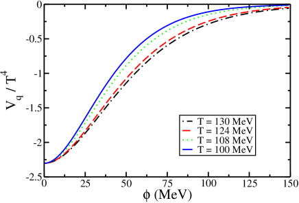
Figure 1: $V_{q}(\phi)$ for different values of the temperature at $\mu_{q}=0$ and for $g=5.5$.

This kind of effective potential is commonly used as the coarse-grained thermodynamic potential in a phenomenological description of the chiral transition for an expanding quark-gluon plasma created in a high-energy heavy-ion collision Scavenius:1999zc ; Scavenius:2000qd ; Scavenius:2001bb ; paech . From the modified field equation (12), one can study, for instance, the phenomena of bubble nucleation and spinodal decomposition. However, the presence of a non-trivial background field configuration, e.g. a bubble, can in principle dramatically modify the Dirac spectrum rajaraman , hence the determinant. In the case of condensed matter systems, where electronic doping often plays a major role, the presence of fermionic bound states can deeply affect the dynamics of the phase transition. This is the case in the presence of a bubble background, where besides unstable critical bubbles one can find metastable configurations, depending on the relative occupation of bound states, and a modification in the value of the nucleation rate Fraga:1994xd ; yulu ; polarons . In the case of a chiral model, analogous effects can in principle appear for a nonzero quark chemical potential. In any case, one expects the effective potential to be modified by the effect of fluctuations of the chiral field on the fermionic density, which motivates the investigation of the next term in the expansion, which contains some information about the inhomogeneity of the bosonic field.

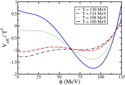
Figure 2: $V_{eff}(\phi)$ in the $\sigma$ direction for different values of the temperature at $\mu_{q}=0$ and for $g=5.5$.

IV.2 First corrections

The next non-trivial term in the expansion contains two contributions: one coming from $\rho_{1}$ and another from $\rho_{2}$. This is due to the rearrangement of powers of the gradient operator. This term will correct the Laplacian piece in the chiral field equation. Dropping zero-temperature contributions which can be absorbed by a redefinition of the bare parameters in $V$, a long but straightforward calculation yields

$$(\rho_{1}+\rho_{2})=-(\nabla^{2}M)~{}W_{q}(T,\mu_{q},\phi)\;,$$ (14)

where

$$W_{q}(T,\mu_{q},\phi)=\frac{\nu_{q}}{2\pi^{2}}\int_{0}^{\infty}~{}dk~{}k^{2}[H(E_{k},T,\mu_{q})+H(E_{k},T,-\mu_{q})]\;,$$ (15)

$$H(E_{k},\mu_{q},\beta) = -\;\beta^{4}\left(\frac{\hat{M}^{4}}{12}\frac{\vec{k}^{2}}{E_{k}^{5}}\right)\left(e^{4\beta(E_{k}-\mu_{q})}-11e^{3\beta(E_{k}-\mu_{q})}+11e^{2\beta(E_{k}-\mu_{q})}-e^{\beta(E_{k}-\mu_{q})}\right)n_{F}^{5}(E_{k},\mu_{q})$$

$$\!\!\!\!-\beta^{3}\left(\frac{\hat{M}^{2}}{24}\frac{\vec{k}^{2}}{E_{k}^{4}}+\frac{5\hat{M}^{4}}{6}\frac{\vec{k}^{2}}{E_{k}^{6}}\right)\left(e^{3\beta(E_{k}-\mu_{q})}-4e^{2\beta(E_{k}-\mu_{q})}+e^{\beta(E_{k}-\mu)}\right)n_{F}^{4}(E_{k},\mu_{q})$$

$$\!\!\!\!-\beta^{2}\left(-\frac{\hat{M}^{2}}{16}\frac{1}{E_{k}^{3}}-\frac{1}{24}\frac{\vec{k}^{2}}{E_{k}^{3}}+\frac{\hat{M}^{2}}{4}\frac{\vec{k}^{2}}{E_{k}^{5}}+\frac{15\hat{M}^{4}}{4}\frac{\vec{k}^{2}}{E_{k}^{7}}\right)\left(e^{\beta(E_{k}-\mu_{q})}-e^{2\beta(E_{k}-\mu_{q})}\right)n_{F}^{3}(E_{k},\mu_{q})$$

$$\!\!\!\!-\beta\left(\frac{1}{4}\frac{1}{E_{k}^{2}}-\frac{3\hat{M}^{2}}{16}\frac{1}{E_{k}^{4}}-\frac{1}{8}\frac{\vec{k}^{2}}{E_{k}^{4}}+\frac{5\hat{M}^{2}}{8}\frac{\vec{k}^{2}}{E_{k}^{6}}+\frac{35\hat{M}^{4}}{4}\frac{\vec{k}^{2}}{E_{k}^{8}}\right)\;e^{\beta(E_{k}-\mu)}\;n_{F}^{2}(E_{k},\mu_{q})$$

$$\!\!\!\!-\left(\frac{1}{8}\frac{1}{E_{k}^{3}}-\frac{3}{16}\frac{\hat{M}^{2}}{E_{k}^{5}}-\frac{1}{8}\frac{\vec{k}^{2}}{E_{k}^{5}}+\frac{5\hat{M}^{2}}{8}\frac{\vec{k}^{2}}{E_{k}^{7}}+\frac{35\hat{M}^{4}}{4}\frac{\vec{k}^{2}}{E_{k}^{9}}\right)n_{F}(E_{k},\mu_{q})\quad,$$

and $n_{F}(E_{k},\mu_{q})$ is the Fermi-Dirac distribution. The derivation of $H(E_{k},T,\mu_{q})$ is not particularly illuminating (a few steps are presented in the appendix). However, in the low-temperature limit, corresponding to $\beta M>>1$, the integral above is strongly suppressed for high values of $k$, and the leading term has the much simpler form

$$W_{q}(T,\mu_{q},\phi)\approx\frac{\nu_{q}}{\pi^{2}}\frac{\sqrt{2\pi}}{8}e^{-\beta|M|}(\beta|M|)^{3/2}\,,$$ (17)

which gives a a better idea of the profile of the first inhomogeneity correction. One can already anticipate that it will be concentrated in the same region where the homogeneous correction was significant, i.e. $\beta M<1$ (cf. Fig. 1), being exponentially suppressed for higher values of the field. In fact, a numerical study of the complete $W_{q}$ shows that this function is peaked around $\phi=0$ and non-negligible for $\beta|\phi|<1$ (see Fig. 3).

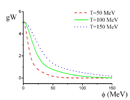
Figure 3: $gW_{q}(\phi)$ for different values of the temperature at $\mu_{q}=0$ and for $g=5.5$.

The Euler-Lagrange equation for the chiral field up to this order in the gradient expansion reads

$$\nabla^{2}\phi=[1+gW_{q}(T,\mu_{q},\phi)]^{-1}~{}\frac{\partial V_{eff}(T,\mu_{q},\phi)}{\partial\phi}\equiv V^{\prime}_{in}(\phi)\;.$$ (18)

Here we used the fact that $(1+gW_{q})$ is a positive definite quantity, and defined a new “effective potential” that contains all the corrections up to this order in the gradient expansion, $V_{in}$. One should not confuse $V_{in}$ with the standard definition of the one-loop effective potential in field theory derived for a constant background itzykson . Nevertheless, we keep the name effective potential for $V_{in}$ for convenience in the description of nucleation that follows.

The complete new effective potential can be obtained from our previous results by numerical integration. In order to proceed analytically, though, we choose to fit its derivative, which we know exactly up to this order, by a polynomial of the fifth degree. Actually, we know that the commonly used effective potential, $V_{eff}=V+V_{q}$, can hardly be distinguished from a fit with a polynomial of sixth degree in the region of interest for nucleation Fraga:2004hp . Working with fits will be most convenient for using well-known results in the thin-wall approximation to estimate physical quantities that are relevant for nucleation, such as the surface tension and the free energy of the critical bubble. Results for the fits of $V^{\prime}_{in}(\phi)$ for $\mu_{q}=0$ are shown in Fig. 4.

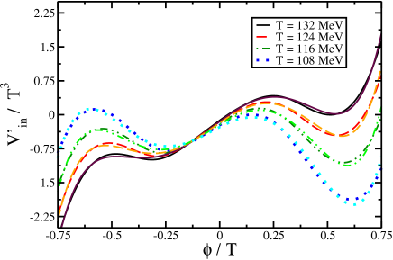
Figure 4: Fits for $V^{\prime}_{in}(\phi)$ for different values of the temperature at $\mu_{q}=0$ and for $g=5.5$. The lines shown in the box correspond to the exact results.

We can now integrate analytically the polynomial approximation to the derivative of the complete effective potential. In Fig. 5 we display the curves for $V_{eff}$ and $V_{in}$ for a few values of temperature and $\mu_{q}=0$.

      

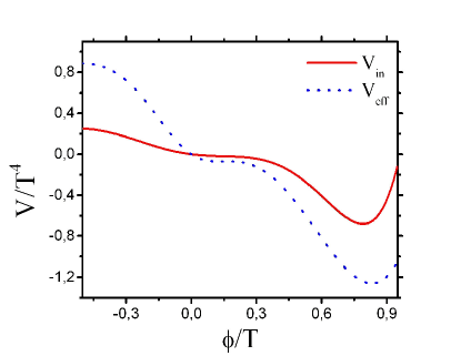
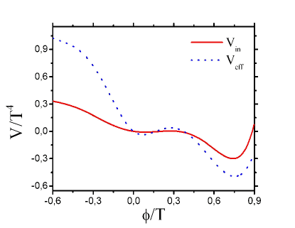
                                (a)                                                                   (b)

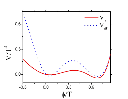
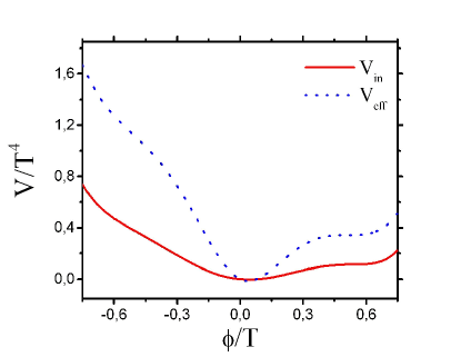
                                (c)                                                                   (d)

Figure 5: $V_{eff}$ and $V_{in}(\phi)$ for different values of the temperature $T=[108~{}{\rm(a)},116~{}{\rm(b)},124~{}{\rm(c)},132~{}{\rm(d)}]$ MeV at $\mu_{q}=0$ and for $g=5.5$.

From Fig. 5 one can notice a few consequences of the inhomogeneity correction. The first general effect is the smoothening of the effective potential. In particular, and most importantly, the barrier between the symmetric phase and the broken phase is significantly diminished, as well as the depth of the broken phase minimum, although we still have a first-order phase transition barrier. Therefore, one can expect an augmentation in the bubble nucleation rate. In principle, one should have better results from calculations within the thin-wall approximation. Also, the critical temperature moves up slightly.

IV.3 Effects on nucleation

Let us now consider the effects of the first inhomogeneity correction on the process of phase conversion driven by the nucleation of bubbles reviews . To work with approximate analytic formulas, we follow Ref. Scavenius:2001bb and express $V_{in}$ over the range $0\leq\phi\leq T$ in the familiar Landau-Ginzburg form

$$V_{\rm eff}\approx\sum_{n=0}^{4}a_{n}\,\Phi^{n}\quad.$$ (19)

Although this approximation is obviously incapable of reproducing all three minima of $V_{in}$, this polynomial form is found to provide a good quantitative description of $V_{in}$ in the region of interest for nucleation, i.e. where the minima for the symmetric and broken phases, as well as the barrier between them, are located.

A quartic potential such as Eq. (19) can always be rewritten in the form

$$U(\varphi)=\alpha~{}(\varphi^{2}-a^{2})^{2}+j\varphi\quad.$$ (20)

The coefficients above are defined as follows:

$$\alpha = a_{4}\quad,$$ (21)

$$a^{2} = \frac{1}{2}\left[-\frac{a_{2}}{a_{4}}+\frac{3}{8}\left(\frac{a_{3}}{a_{4}}\right)^{2}\right]\quad,$$ (22)

$$j = a_{4}\left[\frac{a_{1}}{a_{4}}-\frac{1}{2}\frac{a_{2}}{a_{4}}\frac{a_{3}}{a_{4}}+\frac{1}{8}\left(\frac{a_{3}}{a_{4}}\right)^{3}\right]\quad,$$ (23)

$$\varphi = \phi+\frac{1}{4}\frac{a_{3}}{a_{4}}\ .$$ (24)

The new potential $U(\varphi)$ reproduces the original $V_{in}(\phi)$ up to a shift in the zero of energy. We are interested in the effective potential only between $T_{c}$ and $T_{sp}$. At $T_{c}$, we will have two distinct minima of equal depth. This clearly corresponds to the choice $j=0$ in Eq. (20) so that $U$ has minima at $\varphi=\pm a$ and a maximum at $\varphi=0$. The minimum at $\varphi=-a$ and the maximum move closer together as the temperature is lowered and merge at $T_{sp}$. Thus, the spinodal requires $j/\alpha a^{3}=-8/3\sqrt{3}$ in Eq. (20). The parameter $j/\alpha a^{3}$ falls roughly linearly from $0$, at $T=T_{c}$, to $-8/3\sqrt{3}$ at the spinodal.

The explicit form of the critical bubble in the thin-wall limit is then given by Fraga:1994xd

$$\varphi_{c}(r;\xi,R_{c})=\varphi_{f}+\frac{1}{\xi\sqrt{2\alpha}}\left[1-\tanh\left(\frac{r-R_{c}}{\xi}\right)\right]\quad,$$ (25)

where $\varphi_{f}$ is the new false vacuum, $R_{c}$ is the radius of the critical bubble, and $\xi=2/m$, with $m^{2}\equiv U^{\prime\prime}(\varphi_{f})$, is a measure of the wall thickness. The thin-wall limit corresponds to $\xi/R_{c}\ll 1$ Fraga:1994xd , which can be rewritten as $(3|j|/8\alpha a^{3})\ll 1$. This small parameter has the value of $1/\sqrt{3}$ at the spinodal, which suggests that the thin-wall approximation might be qualitatively reliable for our purposes. Nevertheless, it was shown in Scavenius:2001bb that the thin-wall limit becomes very imprecise as one approaches the spinodal. In this vein, the analysis presented below is to be regarded as semi-quantitative. To be consistent we compare results from the homogeneous calculation to those including the inhomogeneity correction within the same approximation.

In terms of the parameters $\alpha$, $a$, and $j$ defined above, we find

$$\varphi_{t,f} \approx \pm a-\frac{j}{8\alpha a^{2}}\quad,$$ (26)

$$\xi = \left[\frac{1}{\alpha(3\varphi_{f}^{2}-a^{2})}\right]^{1/2}$$ (27)

in the thin-wall limit. Determination of the critical radius requires the surface tension, $\Sigma$, defined as

$$\Sigma\equiv\int_{0}^{\infty}{\rm d}r~{}\left(\frac{{\rm d}\varphi_{b}}{{\rm d}r}\right)^{2}\approx\frac{2}{3\alpha\xi^{3}}\ .$$ (28)

The critical radius then becomes $R_{c}=(2\Sigma/\Delta U)$, where $\Delta U\equiv V(\phi_{f})-V(\phi_{t})\approx 2a|j|$. The free energy of a critical bubble is finally given by $F_{b}=(4\pi\Sigma/3)R_{c}^{2}$. From knowledge of $F_{b}$, one can evaluate the nucleation rate $\Gamma\sim e^{-F_{b}/T}$. In calculating thin-wall properties, we shall use the approximate forms for $\varphi_{t}$, $\varphi_{f}$, $\Sigma$, and $\Delta U$ for all values of the potential parameters.

To illustrate the effect from the inhomogeneity correction, we compute the critical radius and $F_{b}/T$ for three different values of the temperature. For $T=108~{}$MeV, corresponding to the spinodal temperature, which is not modified by the first inhomogeneity correction, the corrected values are $R_{c}\approx 0.98~{}$fm and $F_{b}/T\approx 0.20$, as compared to $R_{c}\approx 1.1~{}$fm and $F_{b}/T\approx 0.9$ in the homogeneous case. The same computation for $T=116~{}$MeV yields $R_{c}\approx 2.15~{}$fm and $F_{b}/T\approx 1.14$, as compared to $R_{c}\approx 2.2~{}$fm and $F_{b}/T\approx 2.1$. At $T=124~{}$MeV, which corresponds to the critical temperature for the homogeneous case, the critical radius and $F_{b}/T$ diverge in the homogeneous computation, whereas $R_{c}\approx 35~{}$fm and $F_{b}/T\approx 394$ including inhomogeneities. The numbers above clearly indicate that the formation of critical bubbles is much less suppressed in the scenario with inhomogeneities, which will in principle accelerate the phase conversion process after the chiral transition.

V Summary and outlook

We have introduced a systematic procedure to evaluate inhomogeneity corrections to the finite-temperature fermionic density in the presence of a chiral background field, which incorporates effects from fluctuations in the bosonic field through a gradient expansion at finite temperature and density. Higher-order contributions give more non-local corrections to the effective Euler-Lagrange equation for the chiral field, and the condition for the validity of the method is a smooth variation of the chiral field, which should be enough in the analysis of its long-wavelength behavior in the phase transition.

Incorporating the first inhomogeneity correction in the computation of the effective potential of the linear $\sigma$-model coupled to quarks, we found that the latter is significantly modified. Besides a general smoothening of the potential, the critical temperature moves upward and the hight of the barrier separating the symmetric and the broken phase vacua diminishes appreciably. As a direct consequence, the radius of the critical bubble goes down, as well as its free energy, and the process of nucleation is facilitated. Although the numbers presented above should be regarded as simple estimates, since they rely on a number of approximations, the qualitative behavior is clear. In a detailed quantitative analysis, one should not only integrate numerically the effective potential and relax the thin-wall approximation, but also include the pion-quark interaction in the computation of the fermionic density. We believe that the contribution from the pion sector will enhance the effect from inhomogeneities.

In all the discussion above, we intentionally ignored corrections coming from bosonic fluctuations, which would result in a bosonic determinant correction to the effective potential bosonic . To focus on the effect of an inhomogeneous background field on the fermionic density, we treated the scalar field essentially as a “heavy” (classical) field, whereas fermions were assumed to be “light”.

Experimental signatures of inhomogeneities for high-energy heavy ion collisions were discussed, for instance, in Refs. paech ; licinio . In particular, inhomogeneities seem to favor an “explosive” scenario explosive for the phase conversion even at early stages of nucleation. However, one should first incorporate dissipation and noise effects, which tend to retard the explosion Fraga:2004hp , before estimating the time scales involved. This analysis will be left for a future publication.

Appendix A

In this appendix we sketch the main steps to build the function $W_{q}(T,\mu_{q},\phi)$ that corrects the Laplacian in the Euler-Lagrange equation for the chiral field.

The first inhomogeneity correction has contributions from $\rho_{1}$ and $\rho_{2}$. The contribution coming from $\rho_{1}$ is proportional to $\nabla_{i}\nabla_{j}\phi$:

$$\rho_{1}^{(2)}(\vec{x})=-Tr_{\gamma}\;\int_{K}\frac{\gamma^{0}k_{0}-\vec{\gamma}\cdot\vec{k}-M(\vec{x})}{k_{0}^{2}-E_{k}^{2}}\left(\frac{1}{2}\nabla_{i}\nabla_{j}M(\vec{x}_{0})\hat{x}^{i}\hat{x}^{j}\right)\left(\frac{\gamma^{0}k_{0}-\vec{\gamma}\cdot\vec{k}-M(\vec{x})}{k_{0}^{2}-E_{k}^{2}}\right)\quad,$$ (29)

where we use a compact notation for the sum-integrals

$$\int_{K}\equiv T\sum_{n}\int\frac{d^{3}k}{(2\pi)^{3}}\quad,$$ (30)

$K\equiv(k_{0},\vec{k})=(i\omega_{n}-\mu_{q},\vec{k})$, and $Tr_{\gamma}$ is a trace over Dirac gamma matrices.

There is also a contribution proportional to $\nabla_{i}\phi\nabla_{j}\phi$ coming from $\rho_{2}$:

$$\rho_{2}^{(1)}(\vec{x})=Tr_{\gamma}\;\int_{K}\frac{\gamma^{0}k_{0}-\vec{\gamma}\cdot\vec{k}-M(\vec{x})}{k_{0}^{2}-E_{k}^{2}}\left[\nabla_{i}M(\vec{x})\hat{x}^{i}\left(\frac{\gamma^{0}k_{0}-\vec{\gamma}\cdot\vec{k}-M(\vec{x})}{k_{0}^{2}-E_{k}^{2}}\right)\right]^{2}\quad.$$ (31)

Up to this order in derivatives, we can write

$$\rho_{1}+\rho_{2} = g\int\frac{d^{3}k}{(2\pi)^{3}}\nu_{q}\left\{\nabla^{2}\hat{M}(\vec{x})\left[F(E_{k},\mu_{q},\beta)+F(E_{k},-\mu_{q},\beta)\right]+(\vec{k}\cdot\nabla)^{2}M(\vec{x})\left[G(E_{k},\mu_{q},\beta)+G(E_{k},-\mu_{q},\beta)\right]\right\}\quad,$$

where $\beta=1/T$,

$$F(E_{k},\mu_{q},\beta)\! = \!-\beta^{2}\left(-\frac{1}{2^{4}}\frac{M^{2}}{E_{k}^{3}}\right)\left(\frac{e^{2\beta(E_{k}-\mu_{q})}-e^{\beta(E_{k}-\mu_{q})}}{(e^{\beta(E_{k}-\mu_{q})}+1)^{3}}\right)$$ (33)

$$-\beta\left(\frac{1}{2^{2}E_{k}^{2}}-\frac{3}{2^{4}}\frac{M^{2}}{E_{K}^{4}}\right)\left(\frac{e^{\beta(E_{k}-\mu_{q})}}{(e^{\beta(E_{k}-\mu_{q})}+1)^{2}}\right)$$

$$-\left(\frac{1}{2^{3}E_{k}^{3}}-\frac{3}{2^{4}}\frac{M^{2}}{E_{K}^{5}}\right)\left(\frac{1}{(e^{\beta(E_{k}-\mu_{q})}+1)}\right)$$

and

$$G(E_{k},\mu_{q},\beta) = -\;\beta^{4}\left(\frac{1}{2^{2}}\frac{M^{4}}{E_{k}^{5}}\right)\left(\frac{e^{4\beta(E_{k}-\mu_{q})}-11e^{3\beta(E_{k}-\mu_{q})}+11e^{2\beta(E_{k}-\mu_{q})}-e^{\beta(E_{k}-\mu_{q})}}{(e^{\beta(E_{k}-\mu_{q})}+1)^{5}}\right)$$ (34)

$$-\beta^{3}\left(\frac{1}{2^{3}}\frac{M^{2}}{E_{K}^{4}}+\frac{5}{2}\frac{M^{4}}{E_{K}^{6}}\right)\left(\frac{e^{3\beta(E_{k}-\mu_{q})}-4e^{2\beta(E_{k}-\mu_{q})}+e^{\beta(E_{k}-\mu_{q})}}{(e^{\beta(E_{k}-\mu_{q})}+1)^{4}}\right)$$

$$-\beta^{2}\left(-\frac{1}{2^{3}E_{K}^{3}}+\frac{3}{2^{2}}\frac{M^{2}}{E_{K}^{5}}+\frac{45}{2^{2}}\frac{M^{4}}{E_{K}^{7}}\right)\left(\frac{e^{2\beta(E_{k}-\mu_{q})}-e^{\beta(E_{k}-\mu_{q})}}{(e^{\beta(E_{k}-\mu_{q})}+1)^{3}}\right)$$

$$-\beta\frac{3}{2^{2}}\left(-\frac{1}{2E_{K}^{4}}+\frac{5}{2}\frac{M^{2}}{E_{K}^{6}}+35\frac{M^{4}}{E_{K}^{8}}\right)\left(\frac{e^{\beta(E_{k}-\mu_{q})}}{(e^{\beta(E_{k}-\mu_{q})}+1)^{2}}\right)$$

$$-\frac{3}{2^{2}}\left(-\frac{1}{2E_{K}^{5}}+\frac{5}{2}\frac{M^{2}}{E_{K}^{7}}+35\frac{M^{4}}{E_{K}^{9}}\right)\left(\frac{1}{(e^{\beta(E_{k}-\mu_{q})}+1)}\right)\quad.$$

Rewriting the term proportional to $\vec{k}\cdot\nabla$ in a more convenient form, using $E_{k}^{2}=\vec{k}^{2}+M^{2}$, and exploring some symmetries in the integrands, it is straightforward to arrive at the final form:

$$\rho_{1}+\rho_{2}=\nabla^{2}\phi(\vec{x})\frac{g\nu_{q}}{2\pi^{2}}\int dk\,\vec{k}^{2}\left[H(E_{k},\mu_{q},\beta)+H(E_{k},-\mu_{q},\beta)\right]\,\,\,,$$ (35)

where

$$H(E_{k},\mu_{q},\beta)\equiv F(E_{k},\mu_{q},\beta)+\frac{1}{3}\vec{k}^{2}\,G(E_{k},\mu_{q},\beta)\,\,\,,$$ (36)

which gives the correction to the Laplacian.

References

- (1) E.V. Shuryak, Phys. Rept. 61, 71 (1980); K. Kajantie and L. McLerran, Ann. Rev. Nucl. Part. Sci. 37, 293 (1987); B. Müller, Rept. Prog. Phys. 58, 611 (1995); J. Harris and B. Müller, Ann. Rev. Nucl. Part. Sci. 46, 71 (1996); S.A. Bass, M. Gyulassy, H. Stöcker and W. Greiner, J. Phys. G25, R1 (1999).
- (2) E.W. Kolb and M.S. Turner, The Early Universe (Addison-Wesley, Redwood City, 1990).
- (3) F. Karsch, Nucl. Phys. A 698, 199 (2002); E. Laermann and O. Philipsen, Ann. Rev. Nucl. Part. Sci. 53, 163 (2003).
- (4) J. Harris and B. Müller, Ann. Rev. Nucl. Part. Sci. 46, 71 (1996).
- (5) Proc. of Quark Matter 2004, J. Phys. G 30, S633-S1425 (2004).
- (6) J. Adams et al. [STAR Collaboration], Phys. Rev. Lett. 91, 072304 (2003).
- (7) L. P. Csernai and I. N. Mishustin, Phys. Rev. Lett. 74, 5005 (1995); A. Abada and J. Aichelin, Phys. Rev. Lett. 74, 3130 (1995); A. Abada and M. C. Birse, Phys. Rev. D 55, 6887 (1997);
- (8) I. N. Mishustin and O. Scavenius, Phys. Rev. Lett. 83, 3134 (1999).
- (9) O. Scavenius and A. Dumitru, Phys. Rev. Lett. 83, 4697 (1999).
- (10) O. Scavenius, A. Mocsy, I. N. Mishustin and D. H. Rischke, Phys. Rev. C 64, 045202 (2001).
- (11) O. Scavenius, A. Dumitru, E. S. Fraga, J. T. Lenaghan and A. D. Jackson, Phys. Rev. D 63, 116003 (2001).
- (12) J. Ignatius, K. Kajantie, H. Kurki-Suonio and M. Laine, Phys. Rev. D 49, 3854 (1994).
- (13) K. Paech, H. Stoecker and A. Dumitru, Phys. Rev. C 68, 044907 (2003); K. Paech and A. Dumitru, Phys. Lett. B 623, 200 (2005).
- (14) C. E. Aguiar, E. S. Fraga and T. Kodama, J. Phys. G 32, 179 (2006).
- (15) R. D. Pisarski, Phys. Rev. D 62, 111501 (2000); A. Dumitru and R. D. Pisarski, Phys. Lett. B 504, 282 (2001); A. Dumitru and R. D. Pisarski, Nucl. Phys. A 698, 444 (2002).
- (16) O. Scavenius, A. Dumitru and A. D. Jackson, Phys. Rev. Lett. 87, 182302 (2001).
- (17) L. P. Csernai and J. I. Kapusta, Phys. Rev. D 46, 1379 (1992).
- (18) M. Gell-Mann and M. Levy, Nuovo Cim. 16, 705 (1960); R. D. Pisarski, Phys. Rev. Lett. 76, 3084 (1996).
- (19) E. S. Fraga and C. A. A. de Carvalho, Phys. Rev. B 52, 7448 (1995).
- (20) J. Kapusta, Finite Temperature Field Theory (Cambridge University Press, Cambridge, 1989).
- (21) A. Dumitru, L. Portugal and D. Zschiesche, nucl-th/0502051; Phys. Rev. C 73, 024902 (2006).
- (22) C. M. Fraser, Z. Phys. C 28, 101 (1985); I. J. R. Aitchison and C. M. Fraser, Phys. Rev. D 31, 2605 (1985).
- (23) Z. Su and B. Sakita, Phys. Rev. B 38, 7421 (1988); P. K. Panigrahi, R. Ray and B. Sakita, ibid. 42, 4036 (1990); C. A. A. de Carvalho, D. G. Barci and L. Moriconi, Phys. Rev. B 50, 4648 (1994); D. G. Barci, E. S. Fraga and C. A. A. de Carvalho, Phys. Rev. D 55, 4947 (1997).
- (24) R. D. Pisarski and F. Wilczek, Phys. Rev. D 29, 338 (1984).
- (25) R. Rajaraman, Solitons and Instantons (North-Holland, 1989).
- (26) Yu-Lu (Ed.), Solitons and Polarons in Conducting Polymers (World Scientific, 1988).
- (27) D. Boyanovsky, C. A. A. de Carvalho and E. S. Fraga, Phys. Rev. B 50, 2889 (1994).
- (28) C. Itzykson and J.-B. Zuber, Quantum Field Theory (Dover Publications, 2006).
- (29) E. S. Fraga and G. Krein, Phys. Lett. B 614, 181 (2005); E. S. Fraga, hep-ph/0510344.
- (30) J. D. Gunton, M. San Miguel and P. S. Sahni, in Phase Transitions and Critical Phenomena (Eds.: C. Domb and J. L. Lebowitz, Academic Press, London, 1983), v. 8.
- (31) T. D. Lee and M. Margulies, Phys. Rev. D 11, 1591 (1975) [Erratum-ibid. D 12, 4008 (1975)]; A. Bochkarev and J. I. Kapusta, Phys. Rev. D 54, 4066 (1996); G. W. Carter, P. J. Ellis and S. Rudaz, III: Mesons Nucl. Phys. A 618, 317 (1997); H. C. G. Caldas, A. L. Mota and M. C. Nemes, Phys. Rev. D 63, 056011 (2001); A. Mocsy, I. N. Mishustin and P. J. Ellis, Phys. Rev. C 70, 015204 (2004).