A theoretical update on $t\bar{t}$ production near threshold

Abstract:

We present an evaluation of the $t\bar{t}$ cross section near threshold at next-to-next-to-leading logarithmic accuracy, using a two-step matching procedure. QED corrections are taken into account as well and are shown to be numerically important. Finally we give an outlook on how to further improve the theoretical predictions with particular emphasis on how to consistently include finite width effects.

1 Introduction

A future International Linear Collider (ILC) offers the opportunity to study the top quark with unprecedented accuracy. To fully exploit the potential of an ILC in this respect, it is essential that a dedicated measurement of the cross section for the production of a top antitop quark pair close to threshold is made. Such a threshold scan allows for an extremely precise measurement of the top-quark mass and yields information on the top-quark width and the top-Higgs Yukawa coupling.

In order to take full advantage of future experimental data, theoretical computations have to match the predicted experimental precision. As is well known [1], a perturbative expansion in the strong coupling $\alpha_{s}$ alone is not adequate due to the presence of terms $(\alpha_{s}/v)^{n}$ at $n$-th order in perturbation theory, where $v\ll 1$ is the (small) velocity of the top quarks near threshold. These terms have to be resummed and the theoretical computations are organized as a double expansion in the two small parameters $\alpha_{s}\sim v$. Thus, a next-to-leading order (NLO) result includes all terms that are suppressed by one power of either $\alpha_{s}$ or $v$, whereas a next-to-next-to-leading order (NNLO) result contains all terms suppressed by either $\alpha_{s}^{2}$, $\alpha_{s}\,v$ or $v^{2}$.

Such an expansion is done most efficiently by using an effective theory approach. From a technical point of view this amounts to using the threshold expansion [2] to split the Feynman diagrams into contributions due to various modes and then integrating out unwanted modes. The modes to be considered are hard modes (with momentum of the order of the heavy quark mass $k^{\mu}\sim m_{t}$), soft modes (with momentum of the order of the typical momentum of the non-relativistic top quarks $k^{\mu}\sim m_{t}\,v$), ultrasoft modes (with momentum of the order of the typical energy of the non-relativistic top quarks $k^{\mu}\sim m_{t}\,v^{2}$) and, finally, potential modes (with $k^{0}\sim m_{t}v^{2}$ and $\vec{k}\sim m_{t}\vec{v}$). In a first step hard modes are integrated out, resulting in non-relativistic QCD (NRQCD) [3]. NRQCD is matched to QCD at a hard scale $\mu_{h}\sim m_{t}$. In a second step, soft modes and potential gluons (and massless quarks) are integrated out. The resulting theory is called potential NRQCD (pNRQCD) [4] and is matched to NRQCD at a soft scale $\mu_{s}\sim m_{t}\,v$. This theory consists of heavy quarks with energy $E\sim m_{t}v^{2}$ and momentum $\vec{k}\sim m_{t}v$, interacting through potentials (to be interpreted as matching coefficients) and still dynamical ultrasoft gluons with momentum $k^{\mu}\sim\mu_{us}\sim m_{t}v^{2}$.

This approach has been used by several groups to compute $t\bar{t}$-pair production near threshold at NNLO (for a review see [5]). If the cross section is expressed in terms of a threshold mass [6, 7] rather than the pole mass, the position of its peak is very stable and can be predicted with a small theoretical error. This will allow to determine the top threshold mass and ultimately the top $\overline{\rm MS}$-mass with a very small error. The situation is much less favourable regarding the normalization of the cross section. The corrections are huge and the scale dependence at NNLO is larger than at NLO, indicating that this quantity is not well under control at NNLO.

The bad behaviour of the fixed order perturbation theory is due to the presence of large logarithms $\log v$. In order to improve the situation, these logarithms have to be resummed. Counting $\alpha\log~{}v\sim 1$ in a NLO and NNLO calculation produces a result of next-to-leading logarithmic (NLL) and next-next-to-leading logarithmic (NNLL) accuracy respectively. At leading order, there are no logarithms. Thus the leading order (LO) result coincides with the result at leading logarithmic accuracy (LL). Within the effective theory approach the logarithms are resummed by computing the anomalous dimensions of the matching coefficients and solving the corresponding renormalization group equations.

The renormalization-group improved (RGI) cross section for $t\bar{t}$ pair production close to threshold has been computed [8] a few years ago using vNRQCD [9], an approach that is somewhat different from the two step matching procedure QCD $\to$ NRQCD $\to$ pNRQCD mentioned above. In vNRQCD the relation between the soft and ultrasoft scale is fixed from the beginning by setting $\mu_{us}=\mu_{s}^{2}/m_{t}$ and there is only one step in the matching procedure, QCD $\to$ vNRQCD. These computations showed that the $\log v$ terms are numerically very important and improve the behaviour of the perturbative series considerably.

So far no calculation of $t\bar{t}$ pair production at NNLL accuracy using a pNRQCD approach has been done, even though most partial results were available for quite a while. In Section 2 we present such a computation [10]. In addition we include QED corrections which turn out to be numerically relevant. The most important missing terms are identified and prospects for future improvements are given in Section 3. A particularly important problem is the inclusion of effects due to the instability of the top quarks. This will be discussed in Section 4 before the conclusions are presented.

2 Current status: $t\bar{t}$ at NNLL

The starting point for the RGI evaluation of the threshold cross section is the fixed-order calculation presented in [11]. The cross section obtains contributions from $\gamma$ and $Z$ exchange. In order to simplify the discussion we ignore the $Z$ exchange in what follows. The cross section at center of mass energy $\sqrt{s}$ can then be written as

$$\sigma^{\gamma}(s)=\frac{4\pi\alpha}{3\,s}\,R(s)$$ (1)

where $\alpha$ is the electromagnetic coupling and the $R$ ratio is expressed as a correlator of two heavy-quark vector currents $j^{\mu}(x)\equiv\bar{Q}\gamma^{\mu}Q(x)$

$$R(s)=\frac{4\pi\,e_{t}^{2}}{s}\,{\rm Im}\left[-i\int d^{4}x\,e^{iqx}\langle 0|T\{j^{\mu}(x)j_{\mu}(0)\}|0\rangle\right]$$ (2)

with $q^{2}=s=(2m_{t}+E)^{2}$ and $e_{t}$ the electric charge of the top. The current is expressed in terms of two-component spinor fields $\psi^{\dagger}$ and $\chi$ resulting in $j\sim c_{1}\,\chi^{\dagger}\sigma^{i}\psi-c_{2}/(6m_{t}^{2})\,\chi^{\dagger}\sigma^{i}\left(i{\bf D}\right)^{2}\psi+\ldots\$. The contributions of the hard modes, which are to be integrated out first, go into the coefficient functions $d_{i}(\mu_{h})$ of the NRQCD Lagrangian and into the matching coefficients of the current $c_{i}(\mu_{h})$. For most coefficients a leading-order result is sufficient, however, $c_{1}$ has to be computed to NNLO [12]. Counting $\alpha\sim\alpha_{s}^{2}$, the one-loop exchange of a hard photon contributes at NNLO and is taken into account by

$$c_{1}(\mu_{h})\to c_{1}(\mu_{h})-\frac{2\,e_{t}^{2}\alpha(\mu_{h})}{\pi}$$ (3)

Once the hard modes are integrated out, we are left with soft, potential and ultrasoft modes. However, near threshold the only allowed external states are potential heavy quarks and ultrasoft gluons. Integrating out the remaining modes results in the pNRCQD Lagrangian, which has the structure

$${\cal L}_{\rm pNRQCD} = {\cal L}^{(0)}_{\rm pNRQCD}+\int d^{3}r\,\left[\psi^{\dagger}T^{a}\psi\right](\vec{x}+\vec{r})\,\delta V\,\left[\chi^{\dagger}T^{a}\chi\right](\vec{x})$$

$$+ \psi^{\dagger}\left(\frac{\partial^{4}}{8m_{t}^{3}}-g_{s}\,\vec{x}\cdot\vec{E}\right)\psi+\chi^{\dagger}\left(-\frac{\partial^{4}}{8m_{t}^{3}}-g_{s}\,\vec{x}\cdot\vec{E}\right)\chi$$

where the leading order Lagrangian

$${\cal L}^{(0)}_{\rm pNRQCD} = \psi^{\dagger}\left(i\partial^{0}+\frac{\partial^{2}}{2m_{t}}+i\Gamma_{t}\right)\psi+\chi^{\dagger}\left(i\partial^{0}-\frac{\partial^{2}}{2m_{t}}+i\Gamma_{t}\right)\chi$$

$$+ \int d^{3}r\,\left[\psi^{\dagger}T^{a}\psi\right](\vec{x}+\vec{r})\left(-\frac{\alpha_{s}}{r}\right)\left[\chi^{\dagger}T^{a}\chi\right](\vec{x})$$

includes the leading Coulomb interaction and takes into account the effects due to the finite width of the top quark by the shift $E\to E+i\Gamma_{t}$. It is known that this does correctly take into account the width effects at leading order, but not at NNLO, an issue we will come back to in Section 4.

The starting point is the free Green function of the Lagrangian ${\cal L}^{(0)}_{\rm pNRQCD}$ which, from a diagramatical point of view, includes all ladder diagrams with the exchange of an arbitrary number of potential gluons. The imaginary part of the Green function at the origin is related to the $R$ ratio by

$$R(E)=\frac{24\pi e_{t}^{2}N_{c}}{s}\,\left(c_{1}^{2}-c_{1}c_{2}\frac{E}{3\,m_{t}}\right)\,{\rm Im}\,G(0,0,E)$$ (6)

where $N_{c}=3$ is the color factor. In order to regularize the ultraviolet singularity present in the Green function, we perform the calculation using dimensional regularization in $D=d+1=4-2\epsilon$ dimensions [11]. After minimal subtraction we obtain [13]

$$G_{c}(0,0,E) \equiv \int\frac{d^{d}p_{1}}{(2\pi)^{d}}\frac{d^{d}p_{2}}{(2\pi)^{d}}\,\tilde{G}_{c}(\vec{p}_{1},\vec{p}_{2},E)$$ (7)

$$= -\frac{\alpha_{s}\,C_{F}\,m_{t}^{2}}{4\pi}\left(\frac{1}{2\lambda}+\frac{1}{2}\ln\frac{-4m_{t}E}{\mu^{2}}-\frac{1}{2}+\gamma_{E}+\psi(1-\lambda)\right)$$

where $\lambda\equiv C_{F}\,\alpha_{s}/(2\sqrt{-E/m_{t}})$ with $C_{F}=4/3$. Once the potential, $\delta V$, is known to the desired accuracy, the NNLO corrections are calculated as single or double insertions

$$\int\frac{d^{d}p_{1}}{(2\pi)^{d}}\frac{d^{d}q_{1}}{(2\pi)^{d}}\frac{d^{d}q_{2}}{(2\pi)^{d}}\frac{d^{d}p_{2}}{(2\pi)^{d}}\,\tilde{G}_{c}(\vec{p}_{1},\vec{q}_{1},E)\,\delta V(\vec{q}_{1}-\vec{q}_{2})\,\tilde{G}_{c}(\vec{q}_{1},\vec{p}_{2},E)$$ (8)

Such insertions can result in divergences. Since the whole calculation is performed using dimensional regularization, it is important that the potentials, to be interpreted as matching coefficients, are computed consistently in $D$ dimensions. Using the result for the two-loop static potential [14], the potential has been computed in Ref. [11]. Here we include an additional contribution in $\delta V$, the electromagnetic Coulomb term

$$\delta V\to\delta V-\frac{4\pi\,e_{t}^{2}\,\alpha}{\vec{q}^{\ 2}}$$ (9)

This will give rise to a NLO term $\sim\alpha/v$ from single potential photon exchange and a NNLO term from double potential photon exchange. We also remark that in Eq. (2) the leading ultrasoft interactions are included [13] even though they only contribute beyond NNLO. They are given by the chromoelectric dipole operator $\vec{x}\cdot\vec{E}(t,0)$ where the electric field is understood to be multipole expanded. An additional term containing $A^{0}(t,0)$ is not displayed since it can be gauged away.

We now turn to the discussion on how to resum the logarithms in this approach. After matching NRQCD to QCD at the hard scale $\mu_{h}$, the renormalization group equations are used to evolve the matching coefficients $d_{i}$ from $d_{i}(\mu_{h})$ to the soft matching scale $d_{i}(\mu_{s})$, thereby resumming logarithms of the form $\log\mu_{h}/\mu_{s}$. The matching coefficients of the single heavy quark sector can be taken from heavy quark effective theory [15]. The RGI coefficients of the four-heavy-quark operators have been computed in Ref. [16].

Matching pNRQCD to NRCQD at the soft scale $\mu_{s}$ then results in potentials that depend on $\alpha_{s}(\mu_{s})$ and the matching coefficients $d_{i}(\mu_{s})$. Again, renormalization group equations are used to evolve the potentials down to ultrasoft scales $\mu_{us}$, resumming $\log\mu_{s}/\mu_{us}$ [16]. This procedure is complicated by the fact that higher dimension operators of the single heavy quark sector can mix through potential loops into lower dimension operators of the heavy quark-antiquark sector. Thus, to obtain the NLL (NNLL) running of $c_{1}$ the NLL (NNLL) running of (some of the) single heavy quark operators has to be taken into account. While all other coefficients are known to an accuracy sufficient for a NNLL calculation, $c_{1}$ is only known to NLL [17]. Some NNLL terms of $c_{1}$ have been computed [18] but we stress that strictly speaking the term NNLL that is commonly used to describe the accuracy of the result is not valid.

From the discussion in the introduction it is clear that the hard, soft and ultrasoft scales are correlated $\mu_{us}\sim\mu_{s}^{2}/\mu_{h}$. As mentioned above, in the vNRQCD approach the scales are fixed by $\mu_{us}=\mu_{s}^{2}/m_{t}$. While the two-step matching procedure in principle does allow to relax this condition, in the current approach, the relation $\mu_{us}=\mu_{s}^{2}/\mu_{h}$ has been used in solving the renormalization group equations. Thus, it is not possible to vary $\mu_{us}$, $\mu_{h}$ and $\mu_{s}$ independently around their natural values. This is somewhat unfortunate, as it would be preferable to have a formulation where the correlation of the scales is not rigid and which would allow to treat and vary the various matching scales independently. This would allow to obtain a more realistic indication of the theoretical error, in particular since some ultrasoft logarithms at NNLL are missing in the present results. For the moment we just have to keep this in mind when trying to assign a theoretical error.

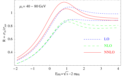
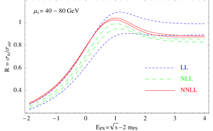
Figure 1: Threshold scan for $t\bar{t}$ using $m_{t,PS}=175$ GeV. The left figure shows the fixed order results, LO, NLO and NNLO, whereas the in right figure the RGI results LL, NLL and NNLL are displayed. The soft scale is varied from $\mu_{s}$=40 GeV to $\mu_{s}$=80 GeV

In Figure 1 the fixed-order results are compared to the RGI results [10] obtained using the procedure described above and using the PS mass [6]. In order to obtain a first rough estimate of the theoretical uncertainty we show the cross sections as bands obtained by variation of the soft scale in the region $40~{}{\rm GeV}\leq\mu_{s}\leq 80~{}{\rm GeV}$ and setting $\mu_{h}=m_{t}$. As was to be expected from previous results [8], the scale dependence is much reduced once the logarithms are taken into account. We also note that the size of the corrections decreases for the RGI results, in particular the NNLL band is much closer to the NNL band, and the scale dependence reduces from LL to NLL to NNLL. However, the NNLL band does not overlap with the NLL band, indicating that a theoretical error estimate relying on the scale variation in this plot alone is too optimistic.

In the fixed-order calculations the by far dominant uncertainty came from the variation of the soft scale. Since this problem is much less severe after the resummation of the logarithms we have to be more careful with other sources of uncertainties. In particular, the missing ultrasoft contributions make it important to consider the dependence on the other scales as well. Since $\mu_{us}$ is related to $\mu_{h}$ by $\mu_{us}=\mu_{s}^{2}/\mu_{h}$, we consider in the left panel of Figure 2 the dependence on $\mu_{h}$ for $\mu_{s}=40$ GeV. Variation of the hard scale around its natural value $\mu_{h}=m_{t}$ by choosing $100~{}{\rm GeV}\leq\mu_{h}\leq 250~{}{\rm GeV}$ results in a scale dependence that is considerably larger than the soft scale dependence. It is to be expected that the situation improves once all ultrasoft logarithms at NNLL are taken into account, but at this stage the rather large dependence of the cross section on $\mu_{h}$ has to be taken into account if a theoretical error is assigned. We also note that the dependence on $\mu_{h}$ only enters at NLL, thus the LL “band” in the left panel of Figure 2 is simply a line.

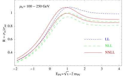
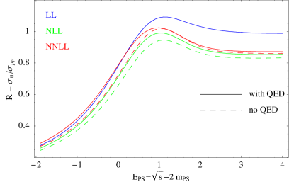
Figure 2: Left panel: Variation of the hard scale $\mu_{h}$ in the threshold scan for $m_{t,PS}=175$ GeV. The hard scale is varied from $100~{}{\rm GeV}\leq\mu_{h}\leq 250~{}{\rm GeV}$. Right panel: the effect of including QED corrections at NLL and NNLL. There are no QED corrections at LL.

Finally we turn to the right panel of Figure 2, where we display the effects due to the QED corrections. As mentioned, they enter at NLL (thus there is no effect on the LL curve) and they are large. They change the normalization by up to 10% and result in a shift in the extracted $\overline{\rm MS}$ mass of up to 100 MeV, making their inclusion imperative.

3 Beyond NNLL

The theoretical error on the peak of the cross section and, with the current RGI results, also its normalization is in rather good shape. Depending on the details of the error analysis, the theoretical error in the determination of the top mass is in the range of 50–150 MeV. The uncertainty in the normalization of the cross section has been quoted as 6% in Ref [8] whereas Figure 2 seems to indicate a somewhat larger value. In any case it is desirable to further reduce the theoretical error, in particular in the determination of the normalization of the cross section, in order to obtain the best possible measurements of the top width and maybe even the top Yukawa coupling.

An obvious first step is to complete the NNLL determination of the current matching coefficient $c_{1}$. Once this is completed, there are two main directions for further improvements. The first concerns the correct implementation of finite width effects and will be discussed in Section 4. The other is the inclusion of corrections of even higher order.

A full NNNLO calculation requires the evaluation of the matching coefficients to the desired order, as well as the computation of the insertions of the potentials. Several partial results have already been obtained. For a start, the logarithmically enhanced NNNLO terms have been obtained a while ago [19]. These terms are included in the NNLL result. Furthermore, the matching coefficient for the non-analytic $1/r^{2}$ potential has been computed to the required accuracy [20] and the NNNLO contribution due to multiple insertions of Coulomb potentials has been computed [21]. However, the calculation of the static potential and the matching coefficient $c_{1}$ of the current are major obstacles on the way to a full NNNLO evaluation.

Of particular importance are the ultrasoft effects. As mentioned before, they enter only at NNNLO and arise due to the emission and absorption of an ultrasoft gluon through the chromoelectric dipole operator. Thus one of the couplings is $\alpha(\mu_{us})$. Since the ultrasoft scale is rather small, it can be argued that these contributions are potentially particularly important NNNLO terms and their evaluation would be an important partial result. Note that this contribution has an ultraviolet singularity, resulting in logarithmically enhanced NNLL terms [19].

The importance of NNNLO contributions can also be seen from the fact that multiple insertions of the Coulomb potential are numerically significant. In Figure 1 the soft scale has not been allowed to run below 40 GeV. The reason is that for $\mu_{s}\leq 30$ GeV the scale dependence get much worse. This bad behaviour is due to the Coulomb potential and it has been shown that including multiple insertions of the Coulomb potential the situation can be rectified [21].

4 Finite width effects

The width of the top quark, $\Gamma_{t}$ is a leading-order effect that has to be taken into account in the propagator of the non-relativistic heavy quarks. This can be seen by noting that the non-relativistic propagator $[E-\vec{p}^{\,2}/(2m_{t})]^{-1}\sim[m_{t}v^{2}]^{-1}$ scales in the same way as the width $\Gamma_{t}\sim m_{t}\alpha_{ew}\sim m_{t}v^{2}$. Thus the suppression due to the insertion of the self energy is compensated by the enhancement of an additional non-relativistic propagator and the corresponding resummation yields

$$\frac{1}{E-\vec{p}^{\ 2}/(2m_{t})}\sum_{n}\left(\frac{-i\,\Gamma_{t}}{E-\vec{p}^{\,2}/(2m_{t})}\right)^{n}=\frac{1}{E+i\,\Gamma_{t}-\vec{p}^{\,2}/(2m_{t})}$$ (10)

This is the justification at leading order of the replacement $E\to E+i\,\Gamma_{t}$. The question is how to go about to include the finite width effects beyond leading order. This question is actually relevant for a large number of processes involving unstable particles, but it is particularly pressing here, given the unprecedented precision required in the theoretical predictions. We recall that the error of the top quark mass $\delta m_{t}\sim 100$ MeV, thus $\delta m_{t}\ll\Gamma_{t}$. Therefore, a systematic approach on how to include finite width effects is mandatory.

To start with we have to emphasise that the very notion of a $t\bar{t}$ cross section breaks down. Taking into account the width effects means we have to take into account the electroweak decay of the top quark. Thus we are dealing with the process $\gamma^{*}\to W^{+}\bar{b}\ W^{-}b$. Even if we neglect the decay of the $W$ bosons, this opens up the possibility of many additional radiative correction processes. There are gluons connecting the intermediate top quarks with the decay products (non-factorizable corrections), there are genuine electroweak corrections and, on top of this all, there are radiative corrections due to photon exchange from any of the decay products with any other charged particle, even the incoming electrons. Some of the electroweak corrections have been taken into account through absorptive parts in the NRQCD matching conditions [22] and have been shown to be numerically relevant. However this does not take all effects into account. In particular QED radiative corrections which are an order $\alpha$ effect and thus contribute at NNLO have to be considered as well in a complete solution to the problem.

The key to the solution is the observation that the situation regarding the finite width corrections is actually very similar to NRQCD. In QCD we have at each order $n$ of perturbation theory terms of the form $(\alpha_{s}/v)^{n}$. Thus the suppression by the coupling is compensated by a kinematic enhancement. This is exactly the same as in Eq. (10). The Coulomb singularity $v=0$ has its analogy in the propagator pole of an on-shell $E=\vec{p}^{\,2}/(2m_{t})$ stable $\Gamma_{t}=0$ top quark. Resummation of the $(\alpha_{s}/v)^{n}$ terms results in a function that is well defined at $v=0$ in the same way as the right hand side of Eq. (10) is well defined for $E=\vec{p}^{\,2}/(2m_{t})$. In NRQCD, the problem of the Coulomb singularity is solved by systematically expanding in both small parameters $\alpha_{s}$ and $v$. Thus the basic idea is to do the same here and use effective theory methods [23] to systematically expand in both small parameters, the coupling and $(p^{2}-m_{t}^{2})/m_{t}^{2}$.

The method has been worked out in detail and its viability has been shown in the case of a toy model with a single resonant heavy scalar particle [24]. A first step towards considering pair production near threshold, albeit for the case of $W$ bosons, has been described in Ref. [25]. However, the main features are the same as for top quark pair production. A consistent description requires the introduction of additional operators and modes. The incoming electrons and the decay products of the top quarks are to be described by collinear modes familiar from soft-collinear effective theory [26]. The production and decay of the top quarks is described by new operators $\left(\bar{e}e\right)\bar{(}\chi^{\dagger}\psi)$, where $\bar{e}$ and $e$ are collinear electron and positron fields respectively, and $\psi^{\dagger}W^{+}b$ and $\chi W^{-}\bar{b}$, where $W$ and $b$ describe the decay products of the top quark. Electroweak corrections are split into various contributions. First there are the hard corrections to be taken into account by computing the matching coefficients of these operators to the desired accuracy. This corresponds to the computation of the matching coefficients in NRQCD and reproduces the so-called factorizable corrections. We are then left with matrix element corrections due to the still dynamical soft, potential and collinear modes which can be associated with the non-factorizable corrections.

While there is still a long way to go to actually perform an explicit calculation, we are confident that this will be the method of choice to include the finite width effects in a systematic way.

5 Conclusions

There has been a lot of progress in the theoretical evaluation of the $t\bar{t}$ threshold cross section and the situation concerning the position of the peak of the cross section, relevant for the mass measurement is very well under control. A mass measurement with an error of 100–150 MeV is certainly achievable, as long as a threshold mass definition is used. Regarding the normalization of the cross section, relevant for a measurement of the width of the top quark and eventually its Yukawa coupling, the resummation of the logarithms has also substantially improved the situation. However, this will need further improvements to fully exploit the potentially very precise experimental data. Apart from the completion of the NNLL evaluation, the effects due to the finite width will have to be fully understood. Obviously, any progress towards a NNNLO evaluation is most welcome. Finally, let me conclude with an obvious but often forgotten remark: exploiting this unique opportunity to measure some Standard Model parameters to an unprecedented accuracy actually does require a dedicated experimental effort in that a future International Linear Collider will have to be run at the top threshold for a reasonable amount of time.

References

-
[1]
V. S. Fadin and V. A. Khoze,
JETP Lett. 46, 525 (1987)
[Pisma Zh. Eksp. Teor. Fiz. 46, 417 (1987)];
V. S. Fadin and V. A. Khoze, Sov. J. Nucl. Phys. 48, 309 (1988) [Yad. Fiz. 48, 487 (1988)]. - [2] M. Beneke and V. A. Smirnov, Nucl. Phys. B 522, 321 (1998) [arXiv:hep-ph/9711391].
-
[3]
W. E. Caswell and G. P. Lepage,
Phys. Lett. B 167, 437 (1986);
G. T. Bodwin, E. Braaten and G. P. Lepage, Phys. Rev. D 51, 1125 (1995) [Erratum-ibid. D 55, 5853 (1997)] [arXiv:hep-ph/9407339]. -
[4]
A. Pineda and J. Soto,
Nucl. Phys. Proc. Suppl. 64, 428 (1998)
[arXiv:hep-ph/9707481];
A. Pineda and J. Soto, Phys. Rev. D 59, 016005 (1999) [arXiv:hep-ph/9805424]. - [5] A. H. Hoang et al., Eur. Phys. J. directC 2, 1 (2000) [arXiv:hep-ph/0001286].
- [6] M. Beneke, Phys. Lett. B 434, 115 (1998) [arXiv:hep-ph/9804241].
-
[7]
I. I. Y. Bigi, M. A. Shifman and N. Uraltsev,
Ann. Rev. Nucl. Part. Sci. 47, 591 (1997)
[arXiv:hep-ph/9703290];
A. H. Hoang, Z. Ligeti and A. V. Manohar, Phys. Rev. Lett. 82, 277 (1999) [arXiv:hep-ph/9809423];
A. Pineda, JHEP 0106 (2001) 022 [arXiv:hep-ph/0105008]. -
[8]
A. H. Hoang, A. V. Manohar, I. W. Stewart and T. Teubner,
Phys. Rev. Lett. 86, 1951 (2001)
[arXiv:hep-ph/0011254];
A. H. Hoang, A. V. Manohar, I. W. Stewart and T. Teubner, Phys. Rev. D 65, 014014 (2002) [arXiv:hep-ph/0107144];
A. H. Hoang, arXiv:hep-ph/0412160. -
[9]
M. E. Luke, A. V. Manohar and I. Z. Rothstein,
Phys. Rev. D 61, 074025 (2000)
[arXiv:hep-ph/9910209];
A. V. Manohar and I. W. Stewart, Phys. Rev. D 62, 014033 (2000) [arXiv:hep-ph/9912226];
A. V. Manohar and I. W. Stewart, Phys. Rev. D 62, 074015 (2000) [arXiv:hep-ph/0003032]. -
[10]
A. Pineda and A. Signer,
arXiv:hep-ph/0601185;
A. Pineda and A. Signer, in preparation. - [11] M. Beneke, A. Signer and V. A. Smirnov, Phys. Lett. B 454, 137 (1999) [arXiv:hep-ph/9903260].
-
[12]
A. Czarnecki and K. Melnikov,
Phys. Rev. Lett. 80, 2531 (1998)
[arXiv:hep-ph/9712222];
M. Beneke, A. Signer and V. A. Smirnov, Phys. Rev. Lett. 80, 2535 (1998) [arXiv:hep-ph/9712302]. - [13] M. Beneke, arXiv:hep-ph/9911490.
-
[14]
Y. Schroder,
Phys. Lett. B 447, 321 (1999)
[arXiv:hep-ph/9812205];
M. Peter, Phys. Rev. Lett. 78, 602 (1997) [arXiv:hep-ph/9610209];
M. Peter, Nucl. Phys. B 501, 471 (1997) [arXiv:hep-ph/9702245]. -
[15]
C. W. Bauer and A. V. Manohar,
Phys. Rev. D 57, 337 (1998)
[arXiv:hep-ph/9708306];
E. Eichten and B. Hill, Phys. Lett. B 243, 427 (1990);
A. F. Falk, B. Grinstein and M. E. Luke, Nucl. Phys. B 357, 185 (1991);
B. Blok, J. G. Korner, D. Pirjol and J. C. Rojas, Nucl. Phys. B 496, 358 (1997) [arXiv:hep-ph/9607233]. - [16] A. Pineda, Phys. Rev. D 65, 074007 (2002) [arXiv:hep-ph/0109117].
- [17] A. Pineda, Phys. Rev. D 66, 054022 (2002) [arXiv:hep-ph/0110216].
-
[18]
B. A. Kniehl, A. A. Penin, M. Steinhauser and V. A. Smirnov,
Phys. Rev. Lett. 90, 212001 (2003)
[arXiv:hep-ph/0210161];
A. H. Hoang, Phys. Rev. D 69, 034009 (2004) [arXiv:hep-ph/0307376];
A. A. Penin, A. Pineda, V. A. Smirnov and M. Steinhauser, Nucl. Phys. B 699, 183 (2004) [arXiv:hep-ph/0406175]. -
[19]
N. Brambilla, A. Pineda, J. Soto and A. Vairo,
Phys. Rev. D 60, 091502 (1999)
[arXiv:hep-ph/9903355];
B. A. Kniehl and A. A. Penin, Nucl. Phys. B 563, 200 (1999) [arXiv:hep-ph/9907489];
N. Brambilla, A. Pineda, J. Soto and A. Vairo, Phys. Lett. B 470, 215 (1999) [arXiv:hep-ph/9910238];
B. A. Kniehl and A. A. Penin, Nucl. Phys. B 577, 197 (2000) [arXiv:hep-ph/9911414]. - [20] B. A. Kniehl, A. A. Penin, M. Steinhauser and V. A. Smirnov, Phys. Rev. D 65, 091503 (2002) [arXiv:hep-ph/0106135].
-
[21]
A. A. Penin, V. A. Smirnov and M. Steinhauser,
Nucl. Phys. B 716, 303 (2005)
[arXiv:hep-ph/0501042];
M. Beneke, Y. Kiyo and K. Schuller, Nucl. Phys. B 714, 67 (2005) [arXiv:hep-ph/0501289]. - [22] A. H. Hoang and C. J. Reisser, Phys. Rev. D 71, 074022 (2005) [arXiv:hep-ph/0412258].
- [23] A. P. Chapovsky, V. A. Khoze, A. Signer and W. J. Stirling, Nucl. Phys. B 621, 257 (2002) [arXiv:hep-ph/0108190].
-
[24]
M. Beneke, A. P. Chapovsky, A. Signer and G. Zanderighi,
Phys. Rev. Lett. 93, 011602 (2004)
[arXiv:hep-ph/0312331];
M. Beneke, A. P. Chapovsky, A. Signer and G. Zanderighi, Nucl. Phys. B 686, 205 (2004) [arXiv:hep-ph/0401002]. - [25] M. Beneke, N. Kauer, A. Signer and G. Zanderighi, arXiv:hep-ph/0411008.
-
[26]
C. W. Bauer, S. Fleming and M. E. Luke,
Phys. Rev. D 63, 014006 (2001)
[hep-ph/0005275];
C. W. Bauer, S. Fleming, D. Pirjol, and I. W. Stewart, Phys. Rev. D63, 114020 (2001) [hep-ph/0011336];
C. W. Bauer, D. Pirjol, and I. W. Stewart, Phys. Rev. D65, 054022 (2002) [hep-ph/0109045];
M. Beneke, A. P. Chapovsky, M. Diehl and Th. Feldmann, Nucl. Phys. B 643, 431 (2002) [hep-ph/0206152].