We analyze the exclusive rare $B\to K^{(*)}\ell^{+}\ell^{-}$, $B\to K^{(*)}\nu\bar{\nu}$ and $B\to K^{*}\gamma$ decays in the Applequist-Cheng-Dobrescu model, which is an extension of the Standard Model in presence of universal extra dimensions. In particular, we consider the case of a single universal extra dimension. We study how spectra, branching fractions and asymmetries depend on the compactification parameter $1/R$, and whether the hadronic uncertainty due to the form factors obscures or not such a dependence. We find that, using present data, it is possible in many cases to put a sensible lower bound to $1/R$, the most stringent one coming from $B\to K^{*}\gamma$. We also study how improved experimental data can be used to establish stronger constraints to this model.

Exclusive $B\to K^{(*)}\ell^{+}\ell^{-}$, $B\to K^{(*)}\nu{\bar{\nu}}$ and $B\to K^{*}\gamma$ transitions
in a scenario with a single Universal Extra Dimension

I Introduction

Although the Standard Model (SM) of electroweak interactions has successfully passed several experimental tests, it is commonly believed that a more fundamental theory should exist. Direct evidence of new Physics will be hopefully gained at high energy colliders such as the LHC. In the meanwhile, signals of new interactions and particles can be obtained indirectly through the analysis of processes which are rare or even forbidden in the Standard Model. Among these, rare B decays induced by $b\to s$ transition play a peculiar role since they are induced at loop level and hence they are suppressed in the Standard Model.

Present data show that such a suppression indeed occurs. In the case of $b\to s\gamma$ modes, which in SM are induced by the electromagnetic penguin diagrams dominated by top and W exchange, the branching fractions have been measured both for inclusive and exclusive transitions; we collect them in Table 1.

Table 1: Branching fractions of rare B decays induced by $b\to s\gamma$ transition.

Mode	Belle Collab.		BaBar Collab.
$B\to X_{s}\gamma$	$(3.55\pm 0.32\pm^{0.30}_{0.31}\pm^{0.11}_{0.07})\times 10^{-4}$	Koppenburg:2004fz	$(3.27\pm 0.18\pm^{0.55}_{0.40}\pm^{0.04}_{0.09})\times 10^{-4}$	Aubert:2005cu
$B^{0}\to K^{*0}\gamma$	$(4.01\pm 0.21\pm 0.17)\times 10^{-5}$	Nakao:2004th	$(3.92\pm 0.20\pm 0.24)\times 10^{-5}$	Aubert:2004te
$B^{-}\to K^{*-}\gamma$	$(4.25\pm 0.31\pm 0.24)\times 10^{-5}$	Nakao:2004th	$(3.87\pm 0.28\pm 0.26)\times 10^{-5}$	Aubert:2004te

Modes with two leptons in the final state, such as $B\to X_{s}\ell^{+}\ell^{-}$, $B\to K^{(*)}\ell^{+}\ell^{-}$ and $B\to X_{s}\nu\bar{\nu}$, $B\to K^{(*)}\nu\bar{\nu}$, are also suppressed. $b\to s\ell^{+}\ell^{-}$ transitions are described in SM by QCD, magnetic and electroweak semileptonic penguin operators, which give rise to an effective Hamiltonian composed of ten operators, as we shall see in more detail below. The resulting SM predictions depend on both the chirality structure of such operators, both on the value of their Wilson coefficients. The situation is simpler in the case of $b\to s\nu{\bar{\nu}}$ modes, described by $Z$ penguin and box diagram dominated by top exchange: the corresponding effective Hamiltonian is composed by a single operator, therefore new Physics effects can just induce an operator with opposite chirality or modify the value of the Wilson coefficient, a scenario relatively simple to analyse.

From the experimental point of view, the most recent measurements of the branching fractions are provided by Belle Iwasaki:2005sy ; Abe:2004ir and BaBar Aubert:2004it ; Aubert:2005cf Collaborations and are collected in Table 2.

Table 2: Branching fractions of rare B decays induced by $b\to s\ell^{+}\ell^{-}$ and $b\to s\nu{\bar{\nu}}$ transitions.

Mode	Belle Collab.		BaBar Collab.
$B\to X_{s}\ell^{+}\ell^{-}$	$(4.11\pm 0.83\pm^{0.85}_{0.81})\times 10^{-6}$	Iwasaki:2005sy	$(5.6\pm 1.5\pm 0.6\pm 1.1)\times 10^{-6}$	Aubert:2004it
$B\to K^{*}\ell^{+}\ell^{-}$	$(16.5\pm^{2.3}_{2.2}\pm 0.9\pm 0.4)\times 10^{-7}$	Abe:2004ir	$(7.8\pm^{1.9}_{1.7}\pm 1.2)\times 10^{-7}$	Aubert:2005cf
$B\to K\ell^{+}\ell^{-}$	$(5.50\pm^{0.75}_{0.70}\pm 0.27\pm 0.02)\times 10^{-7}$	Abe:2004ir	$(3.4\pm 0.7\pm 0.3)\times 10^{-7}$	Aubert:2005cf
$B\to X_{s}\nu\bar{\nu}$
$B\to K^{*}\nu\bar{\nu}$
$B^{-}\to K^{-}\nu\bar{\nu}$	$<3.6\times 10^{-5}\,\,(90\%\,\,CL)$	Abe:2005bq	$<5.2\times 10^{-5}\,\,\,\,(90\%\,\,CL)$	Aubert:2004ws

In addition, important information can be gained from the forward-backward lepton asymmetry in $B\to K^{*}\ell^{+}\ell^{-}$, which is a powerful tool to distinguish between SM and several extensions of it. Belle Collaboration has recently provided the first measurement of such an asymmetry Abe:2005km .

Among the various models of Physics beyond the SM, those with extra dimensions are attracting interest for manifold reasons. For example, they provide a unified framework for gravity and other interactions, giving some hints on the hierarchy problem and a connection with string theory. Particularly interesting are the scenarios with universal extra dimensions, in which all the SM fields are allowed to propagate in the extra dimensions. Their feature is that compactification of the extra dimensions leads to the appearance of Kaluza-Klein (KK) partners of the SM fields in the four dimensional description of the higher dimensional theory, together with KK modes without corresponding SM partners. A simple scenario is represented by the Appelquist-Cheng-Dobrescu (ACD) model Appelquist:2000nn with a single compactified extra dimension, which presents the appealing feature of introducing only one additional free parameter with respect to the Standard Model, i.e. $1/R$, the inverse of the compactification radius.

Analyses aimed at identifying the signatures of extra dimensions in processes already accessible at particle accelerators or within the reach of future facilities give different bounds to the sizes of extra dimensions, depending on the specific model considered. The bounds are more severe in the case of UED, and in the 5-d scenario constraints from Tevatron run I allow to put the bound $1/R\geq 300$ GeV. In the following we analyze a broader range $1/R\geq 200$ GeV to be more general.

Rare $B$ transitions can be used to constrain the ACD scenario Agashe:2001xt . In particular, Buras and collaborators have investigated the impact of universal extra dimensions on the $B^{0}_{d,s}-\bar{B}^{0}_{d,s}$ mixing mass differences, on the CKM unitarity triangle and on inclusive $b\to s$ decays for which they have computed the effective Hamiltonian Buras:2002ej ; Buras:2003mk . The availability of precise data on exclusive $b\to s$-induced decays, collected in Tables 1,2, induces us to extend the analysis to such processes in the framework of the ACD model. In this case, the uncertainty in the hadronic form factors must be taken into account, since it can overshadow the sensitivity to the compactification parameter. Actually, we show that this is not the case, at least for the smallest values of $1/R$: computing, for example, the branching fractions of $B\to K^{(*)}\ell^{+}\ell^{-}$ as well as the forward-backward lepton asymmetry in $B\to K^{*}\ell^{+}\ell^{-}$ for a representative set of form factors we find that a bound can be put, and it can be improved following the improvements in the experimental data. Moreover, since in the limit of large $1/R$ the Standard Model is recovered, we also investigate the agreement of current data with SM predictions Hurth:2003vb . We have also considered the decays $B\to K^{(*)}\nu\bar{\nu}$, although for these modes no signal has been observed, so far, studying how observables like the various helicity amplitudes for $B\to K^{*}$ transitions are modified in the ACD model. Finally, we have considered the branching fraction of $B\to K^{*}\gamma$ as a function of $1/R$, pointing out that it allows to establish the most stringent bound for the compactification parameter.

The plan of the paper is as follows: in the next Section we briefly describe the ACD model. We discuss the modes $B\to K^{(*)}\ell^{+}\ell^{-}$, $B\to K^{(*)}\nu\bar{\nu}$ and $B\to K^{*}\gamma$ in the subsequent Sections; finally, we present our conclusions and the perspectives for further analyses.

II Models with extra dimensions: the ACD model with a single UED

If other dimensions exist in our universe apart the usual 3 spatial + 1 temporal ones, and if such extra dimensions are compactified, fields living in all dimensions would manifest themselves in the 3+1 space by the appearence of Kaluza-Klein excitations (from the original Kaluza and Klein studies aimed at unifying electromagnetism and gravity by the introduction of one extra dimension KK ). For example, in the case of a single extra dimension with coordinate $x_{5}=y$ compactified on a circle of radius R (the compactification radius), a field $F(x,y)$ (with $x$ denoting the whole of the usual 3+1 coordinates) would be a periodic function of $y$, and hence it could be expressed as

$$F(x,y)=\sum_{n=-\infty}^{n=+\infty}F_{n}(x)e^{i\,n\cdot y/R}\,\,\,.$$ (1)

If, for example, $F$ is a boson field obeying the equation of motion $\partial_{M}\partial^{M}F(x,y)=0$ (M=0,1,2,3,5), the KK modes $F_{n}$ would obey the equation

$$\left(\partial^{\mu}\partial_{\mu}+{n^{2}\over R^{2}}\right)F_{n}(x)=0\,\,\,\hskip 28.45274pt\mu=0,1,2,3\,\,\,,$$ (2)

and therefore, apart the zero mode, they would behave in four dimensions as massive particles with $m_{n}^{2}=(n/R)^{2}$.

An important question is whether ordinary fields propagate or not in all the dimensions. One possibility is that only gravity propagates in the whole ordinary + extra dimensional Universe, the ”bulk”. Opposed to this are models with universal extra dimensions (UED), in which all the fields propagate in all available dimensions.

In this paper we focus on the model developed by Appelquist, Cheng and Dobrescu (ACD) Appelquist:2000nn that belongs to the UED scenarios. It consists in the minimal extension of the SM in $4+\delta$ dimensions, and we consider the simplest case $\delta=1$. This extra dimension is compactified to the orbifold $S^{1}/Z_{2}$, with the coordinate $x_{5}=y$ running from 0 to $2\pi R$. The points $y=0,y=\pi R$ are fixed points of the orbifold; the boundary conditions at these points determine the Kaluza Klein mode expansion of the fields. Under the parity transformation $P_{5}:y\to-y$ fields having a correspondent in the 4-d SM should be even, so that their zero mode in the KK mode expansion can be interpreted as the ordinary SM field. On the other hand, fields having no correspondent in the SM should be odd, and therefore they do not have zero modes in the KK expansion. For example, in this scenario a vector field has a fifth component which is odd under $P_{5}$.

Important features of the ACD model are: i) there is a single additional free parameter with respect to the SM, the compactification radius $R$; ii) the conservation of KK parity, which has the consequence that there is no tree-level contribution of KK modes in low energy processes (at scales $\mu\ll 1/R$) and no production of single KK excitation in ordinary particle interactions.

A detailed description of the extension of SM in five dimensions is provided in Buras:2002ej ; here we recall the main features of such a construction.

• Gauge group

  The gauge bosons associated to $SU(2)_{L}\times U(1)_{Y}$ gauge group are $W_{M}^{a}$ ($a=1,2,3$, $M=0,1,2,3,5$) and $B_{M}$, and the gauge couplings are: ${\hat{g}}_{2}=g_{2}\sqrt{2\pi R}$ and ${\hat{g}}^{\prime}=g^{\prime}\sqrt{2\pi R}$ (we denote with the caret the quantities referring to the five dimensional description). The charged bosons are $W_{M}^{\pm}={1\over\sqrt{2}}(W_{M}^{1}\mp W_{M}^{2})$. Moreover, as in SM, $W_{M}^{3}$ and $B_{M}$ mix giving rise to the fields $Z_{M}$ and $A_{M}$. The mixing angle is defined through the ordinary relations:

  $$c_{W}=\cos\theta_{W}={{\hat{g}}_{2}\over\sqrt{{\hat{g}}_{2}^{2}+{\hat{g}}^{\prime 2}}}\hskip 28.45274pts_{W}=\sin\theta_{W}={{\hat{g}}^{\prime}\over\sqrt{{\hat{g}}_{2}^{2}+{\hat{g}}^{\prime 2}}}\,\,\,.$$ (3)

  Due to the relations between the five and four dimensional gauge constants, the Weinberg angle is the same as in SM. On the other hand, the gauge bosons associated to $SU(3)_{c}$ are the gluons $G^{a}_{M}(x,y)$ ($a=1,..,8$).

• Higgs sector

  The Higgs doublet is written as:

  $$\phi=\left(\begin{array}[]{c}i\chi^{+}\\ {1\over\sqrt{2}}(\psi-i\chi_{3})\end{array}\right)$$ (4)

  where $\chi^{\pm}={1\over\sqrt{2}}(\chi^{1}\mp\chi^{2})$. Among these fields only $\psi$ has a zero mode, and we assign to such a mode a vacuum expectation value ${\hat{v}}$, so that $\psi\to{\hat{v}}+H$. $H$ can be identified with the SM Higgs field, while the vacuum expectation value in 5 dimensions is related to the corresponding quantity in 4 dimensions through the relation: $\hat{v}={v/\sqrt{2\pi R}}$.

• Mixing between Higgs fields and gauge bosons

  The charged $W_{5(n)}^{\pm}$ and $\chi^{\pm}_{(n)}$ fields mix, as well as the neutral $Z_{5(n)}$ and $\chi_{3(n)}$. The resulting fields are $G_{(n)}^{0}$, $G_{(n)}^{\pm}$ which are Goldstone modes giving mass to the $W_{(n)}^{\pm\mu}$ and $Z_{(n)}^{\mu}$, and $a_{(n)}^{0}$, $a_{(n)}^{\pm}$, new physical scalars.

• Yukawa terms

  In order to have chiral fermions as in the SM, the left and the right-handed components of a given spinor cannot be simultaneously even under $P_{5}$. The Yukawa coupling of the Higgs field to the fermions provides the fermion mass terms, and the diagonalization of such terms leads to the introduction of the CKM matrix, with the same steps as in the SM. In this respect, the ACD model belongs to the class of minimal flavour violation models, since there are no new operators beyond those present in the SM and no new phases beyond the CKM phase. As a consequence, Buras and collaborators have shown that the unitarity triangle is the same as in the SM Buras:2002ej . In order to obtain 4-d mass eigenstates for the higher KK levels, a further mixing is introduced among the left-handed doublet and the right-handed singlet for each flavour $f$. The mixing angle is such that $\displaystyle\tan(2\alpha_{f(n)})={m_{f}\over n/R}$ ($n\geq 1$) giving the masses $\displaystyle m_{f(n)}=\sqrt{m_{f}^{2}+{n^{2}\over R^{2}}}$, so that it is negligible for all flavours except the top.

As a result of the construction, the four-dimensional Lagrangian, obtained integrating over the 5th dimension $y$:

$${\cal L}_{4}(x)=\int_{0}^{2\pi R}{\cal L}_{5}(x,y)$$ (5)

describes i) zero modes (corresponding to the Standard Model fields), ii) their massive KK excitations, iii) KK excitations without zero modes (they do not correspond to any field in SM). The related Feynman rules can be found in Buras:2002ej .

III Decays $B\to K^{(*)}\ell^{+}\ell^{-}$

In the Standard Model the effective $\Delta B=-1$, $\Delta S=1$ Hamiltonian governing the rare transition $b\to s\ell^{+}\ell^{-}$ can be written in terms of a set of local operators:

$$H_{W}\,=\,4\,{G_{F}\over\sqrt{2}}V_{tb}V_{ts}^{*}\sum_{i=1}^{10}C_{i}(\mu)O_{i}(\mu)$$ (6)

where $G_{F}$ is the Fermi constant and $V_{ij}$ are elements of the Cabibbo-Kobayashi-Maskawa mixing matrix; we neglect terms proportional to $V_{ub}V_{us}^{*}$ since the ratio $\displaystyle\left|{V_{ub}V_{us}^{*}\over V_{tb}V_{ts}^{*}}\right|$ is of the order $10^{-2}$. The operators $O_{i}$, written in terms of quark and gluon fields, read as follows:

$$O_{1} = ({\bar{s}}_{L\alpha}\gamma^{\mu}b_{L\alpha})({\bar{c}}_{L\beta}\gamma_{\mu}c_{L\beta})$$

$$O_{2} = ({\bar{s}}_{L\alpha}\gamma^{\mu}b_{L\beta})({\bar{c}}_{L\beta}\gamma_{\mu}c_{L\alpha})$$

$$O_{3} = ({\bar{s}}_{L\alpha}\gamma^{\mu}b_{L\alpha})[({\bar{u}}_{L\beta}\gamma_{\mu}u_{L\beta})+...+({\bar{b}}_{L\beta}\gamma_{\mu}b_{L\beta})]$$

$$O_{4} = ({\bar{s}}_{L\alpha}\gamma^{\mu}b_{L\beta})[({\bar{u}}_{L\beta}\gamma_{\mu}u_{L\alpha})+...+({\bar{b}}_{L\beta}\gamma_{\mu}b_{L\alpha})]$$

$$O_{5} = ({\bar{s}}_{L\alpha}\gamma^{\mu}b_{L\alpha})[({\bar{u}}_{R\beta}\gamma_{\mu}u_{R\beta})+...+({\bar{b}}_{R\beta}\gamma_{\mu}b_{R\beta})]$$

$$O_{6} = ({\bar{s}}_{L\alpha}\gamma^{\mu}b_{L\beta})[({\bar{u}}_{R\beta}\gamma_{\mu}u_{R\alpha})+...+({\bar{b}}_{R\beta}\gamma_{\mu}b_{R\alpha})]$$

$$O_{7} = {e\over 16\pi^{2}}m_{b}({\bar{s}}_{L\alpha}\sigma^{\mu\nu}b_{R\alpha})F_{\mu\nu}$$

$$O_{8} = {g_{s}\over 16\pi^{2}}m_{b}\Big{[}{\bar{s}}_{L\alpha}\sigma^{\mu\nu}\Big{(}{\lambda^{a}\over 2}\Big{)}_{\alpha\beta}b_{R\beta}\Big{]}\;G^{a}_{\mu\nu}$$

$$O_{9} = {e^{2}\over 16\pi^{2}}({\bar{s}}_{L\alpha}\gamma^{\mu}b_{L\alpha})\;{\bar{\ell}}\gamma_{\mu}\ell$$

$$O_{10} = {e^{2}\over 16\pi^{2}}({\bar{s}}_{L\alpha}\gamma^{\mu}b_{L\alpha})\;{\bar{\ell}}\gamma_{\mu}\gamma_{5}\ell$$ (7)

where $\alpha$, $\beta$ are colour indices, $\displaystyle b_{R,L}={1\pm\gamma_{5}\over 2}b$, and $\displaystyle\sigma^{\mu\nu}={i\over 2}[\gamma^{\mu},\gamma^{\nu}]$; $e$ and $g_{s}$ are the electromagnetic and the strong coupling constant, respectively, while $F_{\mu\nu}$ and $G^{a}_{\mu\nu}$ in $O_{7}$ and $O_{8}$ denote the electromagnetic and the gluonic field strength tensor. $O_{1}$ and $O_{2}$ are current-current operators, $O_{3},...,O_{6}$ are QCD penguin operators, $O_{7}$ (inducing the radiative $b\to s\gamma$ decay) and $O_{8}$ are magnetic penguin operators, $O_{9}$ and $O_{10}$ are semileptonic electroweak penguin operators.

The Wilson coefficients appearing in (6) have been computed at NNLO in the Standard Model nnlo . At NLO the coefficients have been computed also for the ACD model including the effects of KK modes Buras:2002ej ; Buras:2003mk : we use these results in our study. No operators other than those collected in eq.(7) are found in ACD, therefore the whole contribution of the plethora of states only produces a modification of the Wilson coefficients that now depend on the additional ACD parameter, the compactification radius. For large values of $1/R$ the Standard Model phenomenology should be recovered, since the new states, being more and more massive, decouple from the low-energy theory. Our aim is to establish a lower bound on $1/R$ from the various $B\to K^{(*)}\ell^{+}\ell^{-}$ observables.

In the following we do not consider the contribution to $B\to K^{*}\ell^{+}\ell^{-}$ with the lepton pair coming from $c{\bar{c}}$ resonances, which is mainly due to the operators $O_{1}$ and $O_{2}$ in (7). It can be experimentally removed applying appropriate kinematical cuts around the resonances. QCD penguins $O_{3},...,O_{6}$ can also be neglected since their Wilson coefficients are very small compared to the others. Therefore, we only need the coefficients $C_{7}$, $C_{9}$ and $C_{10}$: as discussed in Buras:2002ej ; Buras:2003mk , the impact of the KK modes consists in the enhancement of $C_{10}$ and the suppression of $C_{7}$.

The Wilson coefficients in ACD are modified because particles not present in SM can contribute as intermediate states in penguin and box diagrams. As a consequence, the Wilson coefficients can be expressed in terms of functions $F(x_{t},1/R)$, $x_{t}=\displaystyle{m_{t}^{2}\over M_{W}^{2}}$, which generalize the corresponding SM functions $F_{0}(x_{t})$ according to:

$$F(x_{t},1/R)=F_{0}(x_{t})+\sum_{n=1}^{\infty}F_{n}(x_{t},x_{n})$$ (8)

where $x_{n}=\displaystyle{m_{n}^{2}\over M_{W}^{2}}$ and $m_{n}=\displaystyle{n\over R}$. The relevant functions are the following: $C(x_{t},1/R)$ from $Z^{0}$ penguins; $D(x_{t},1/R)$ from $\gamma$ penguins; $E(x_{t},1/R)$ from gluon penguins; $D^{\prime}(x_{t},1/R)$ from $\gamma$ magnetic penguins; $E^{\prime}(x_{t},1/R)$ from chromomagnetic penguins. The functions can be found in Buras:2002ej ; Buras:2003mk ; here we collect the formulae needed in our analysis.

• $C_{7}$

  In place of $C_{7}$, one defines an effective coefficient $C_{7}^{(0)eff}$ which is renormalization scheme independent Buras:1993xp :

  $$C_{7}^{(0)eff}(\mu_{b})=\eta^{16\over 23}C_{7}^{(0)}(\mu_{W})+{8\over 3}\left(\eta^{14\over 23}-\eta^{16\over 23}\right)C_{8}^{(0)}(\mu_{W})+C_{2}^{(0)}(\mu_{W})\sum_{i=1}^{8}h_{i}\eta^{\alpha_{i}}$$ (9)

  where $\displaystyle\eta={\alpha_{s}(\mu_{W})\over\alpha_{s}(\mu_{b})}$, and

  $$C_{2}^{(0)}(\mu_{W})=1\hskip 14.22636ptC_{7}^{(0)}(\mu_{W})=-{1\over 2}D^{\prime}(x_{t},1/R),\hskip 14.22636ptC_{8}^{(0)}(\mu_{W})=-{1\over 2}E^{\prime}(x_{t},1/R);$$ (10)

  the superscript $(0)$ stays for leading log approximation. Furthermore:

  $$a_{1}={14\over 23}\hskip 11.38092pta_{2}={16\over 23}\hskip 11.38092pt a_{3}={6\over 23}\hskip 11.38092pta_{4}=-{12\over 23}$$

  $$a_{5}=0.4086\hskip 11.38092pta_{6}=-0.4230\hskip 11.38092pt a_{7}=-0.8994\hskip 11.38092pta_{8}=0.1456$$

  $$h_{1}=2.2996\hskip 11.38092pth_{2}=-1.0880\hskip 11.38092pt h_{3}=-{3\over 7}\hskip 11.38092pth_{4}=-{1\over 14}$$ (11)

  $$h_{5}=-0.6494\hskip 11.38092pth_{6}=-0.0380\hskip 11.38092pt h_{7}=-0.0185\hskip 11.38092pth_{8}=-0.0057\,\,\,.$$

  The functions $D^{\prime}$ and $E^{\prime}$ are given by eq. (8) with

  $$D^{\prime}_{0}(x_{t})=-{(8x_{t}^{3}+5x_{t}^{2}-7x_{t})\over 12(1-x_{t})^{3}}+{x_{t}^{2}(2-3x_{t})\over 2(1-x_{t})^{4}}\ln x_{t}$$ (12)

  $$E^{\prime}_{0}(x_{t})=-{x_{t}(x_{t}^{2}-5x_{t}-2)\over 4(1-x_{t})^{3}}+{3x_{t}^{2}\over 2(1-x_{t})^{4}}\ln x_{t}$$ (13)

  $$D^{\prime}_{n}(x_{t},x_{n}) = {x_{t}(-37+44x_{t}+17x_{t}^{2}+6x_{n}^{2}(10-9x_{t}+3x_{t}^{2})-3x_{n}(21-54x_{t}+17x_{t}^{2}))\over 36(x_{t}-1)^{3}}$$

  $$+ {x_{n}(2-7x_{n}+3x_{n}^{2})\over 6}\ln{x_{n}\over 1+x_{n}}$$

  $$- {(-2+x_{n}+3x_{t})(x_{t}+3x_{t}^{2}+x_{n}^{2}(3+x_{t})-x_{n}(1+(-10+x_{t})x_{t}))\over 6(x_{t}-1)^{4}}\ln{x_{n}+x_{t}\over 1+x_{n}}$$

  $$E^{\prime}_{n}(x_{t},x_{n}) = {x_{t}(-17-8x_{t}+x_{t}^{2}-3x_{n}(21-6x_{t}+x_{t}^{2})-6x_{n}^{2}(10-9x_{t}+3x_{t}^{2}))\over 12(x_{t}-1)^{3}}$$ (15)

  $$- {1\over 2}x_{n}(1+x_{n})(-1+3x_{n})\ln{x_{n}\over 1+x_{n}}$$

  $$+ {(1+x_{n})(x_{t}+3x_{t}^{2}+x_{n}^{2}(3+x_{t})-x_{n}(1+(-10+x_{t})x_{t}))\over 2(x_{t}-1)^{4}}\ln{x_{n}+x_{t}\over 1+x_{n}}\,\,\,.$$

  Following Buras:2002ej one gets the expressions for the sum over $n$:

  $$\sum_{n=1}^{\infty}D^{\prime}_{n}(x_{t},x_{n}) = -{x_{t}(-37+x_{t}(44+17x_{t}))\over 72(x_{t}-1)^{3}}$$

  $$+{\pi M_{W}R\over 2} \Bigg{[}\int_{0}^{1}dy\,{(2y^{1/2}+7y^{3/2}+3y^{5/2})\over 6}\coth(\pi M_{W}R\sqrt{y})$$ (16)

  $$+ {(-2+3x_{t})x_{t}(1+3x_{t})\over 6(x_{t}-1)^{4}}J(R,-1/2)$$

  $$- {1\over 6(x_{t}-1)^{4}}\left[x_{t}(1+3x_{t})-(-2+3x_{t})(1+(-10+x_{t})x_{t})\right]J(R,1/2)$$

  $$+ {1\over 6(x_{t}-1)^{4}}\left[(-2+3x_{t})(3+x_{t})-(1+(-10+x_{t})x_{t})\right]J(R,3/2)$$

  $$- {(3+x_{t})\over 6(x_{t}-1)^{4}}J(R,5/2)\Bigg{]}$$

  $$\sum_{n=1}^{\infty}E^{\prime}_{n}(x_{t},x_{n}) = -{x_{t}(-17+(-8+x_{t})x_{t})\over 24(x_{t}-1)^{3}}$$

  $$+{\pi M_{W}R\over 4} \Bigg{[}\int_{0}^{1}dy\,(y^{1/2}+2y^{3/2}-3y^{5/2})\,\coth(\pi M_{W}R\sqrt{y})$$ (17)

  $$- {x_{t}(1+3x_{t})\over(x_{t}-1)^{4}}J(R,-1/2)$$

  $$+ {1\over(x_{t}-1)^{4}}\left[x_{t}(1+3x_{t})-(1+(-10+x_{t})x_{t})\right]J(R,1/2)$$

  $$- {1\over(x_{t}-1)^{4}}\left[(3+x_{t})-(1+(-10+x_{t})x_{t})\right]J(R,3/2)$$

  $$+ {(3+x_{t})\over(x_{t}-1)^{4}}J(R,5/2)\Bigg{]}$$

  where

  $$J(R,\alpha)=\int_{0}^{1}dy\,y^{\alpha}\left[\coth(\pi M_{W}R\sqrt{y})-x_{t}^{1+\alpha}\coth(\pi m_{t}R\sqrt{y})\right]\,\,\,.$$ (18)

• $C_{9}$

  In the ACD model and in the NDR scheme one has

  $$C_{9}(\mu)=P_{0}^{NDR}+{Y(x_{t},1/R)\over\sin^{2}\theta_{W}}-4Z(x_{t},1/R)+P_{E}E(x_{t},1/R)$$ (19)

  where $P_{0}^{NDR}=2.60\pm 0.25$ Misiak:1992bc and the last term is numerically negligible. Besides

  $$Y(x_{t},1/R) = Y_{0}(x_{t})+\sum_{n=1}^{\infty}C_{n}(x_{t},x_{n})$$

  $$Z(x_{t},1/R) = Z_{0}(x_{t})+\sum_{n=1}^{\infty}C_{n}(x_{t},x_{n})$$ (20)

  with

  $$Y_{0}(x_{t}) = {x_{t}\over 8}\left[{x_{t}-4\over x_{t}-1}+{3x_{t}\over(x_{t}-1)^{2}}\ln x_{t}\right]\,\,$$

  $$Z_{0}(x_{t}) = {18x_{t}^{4}-163x_{t}^{3}+259x_{t}^{2}-108x_{t}\over 144(x_{t}-1)^{3}}$$ (21)

  $$+ \left[{32x_{t}^{4}-38x_{t}^{3}-15x_{t}^{2}+18x_{t}\over 72(x_{t}-1)^{4}}-{1\over 9}\right]\ln x_{t}\,\,$$

  $$C_{n}(x_{t},x_{n})=\frac{x_{t}}{8(x_{t}-1)^{2}}\left[x_{t}^{2}-8x_{t}+7+(3+3x_{t}+7x_{n}-x_{t}x_{n})\ln\frac{x_{t}+x_{n}}{1+x_{n}}\right]$$ (22)

  and

  $$\sum_{n=1}^{\infty}C_{n}(x_{t},x_{n})=$$

  $${x_{t}(7-x_{t})\over 16(x_{t}-1)}-{\pi M_{W}Rx_{t}\over 16(x_{t}-1)^{2}}\left[3(1+x_{t})J(R,-1/2)+(x_{t}-7)J(R,1/2)\right]\,\,\,.$$ (23)

• $C_{10}$

  $C_{10}$ is $\mu$ independent and is given by

  $$C_{10}=-{Y(x_{t},1/R)\over\sin^{2}\theta_{W}}\,\,\,\,.$$ (24)

We fix the renormalization scale to $\mu=\mu_{b}\simeq 5$ GeV.

With these coefficients and the operators in (7) the inclusive $b\to s\ell^{+}\ell^{-}$ transitions have been studied in Buras:2002ej ; Buras:2003mk . The exclusive $B\to K^{(*)}\ell^{+}\ell^{-}$ modes, on the other hand, involve the matrix elements of the operators in (7) between the $B$ and $K$ or $K^{*}$ mesons, for which we use the standard parametrization in terms of form factors:

$$<K(p^{\prime})|{\bar{s}}\gamma_{\mu}b|B(p)>=(p+p^{\prime})_{\mu}F_{1}(q^{2})+{M_{B}^{2}-M_{K}^{2}\over q^{2}}q_{\mu}\left(F_{0}(q^{2})-F_{1}(q^{2})\right)$$ (25)

( $q=p-p^{\prime}$, $F_{1}(0)=F_{0}(0)$) and

$$<K(p^{\prime})|{\bar{s}}\;i\;\sigma_{\mu\nu}q^{\nu}b|B(p)>=\Big{[}(p+p^{\prime})_{\mu}q^{2}-(M_{B}^{2}-M_{K}^{2})q_{\mu}\Big{]}\;{F_{T}(q^{2})\over M_{B}+M_{K}}\hskip 3.0pt;$$ (26)

$$<K^{*}(p^{\prime},\epsilon)|{\bar{s}}\gamma_{\mu}(1-\gamma_{5})b|B(p)> = \epsilon_{\mu\nu\alpha\beta}\epsilon^{*\nu}p^{\alpha}p^{\prime\beta}{2V(q^{2})\over M_{B}+M_{K^{*}}}$$ (27)

$$- i\left[\epsilon^{*}_{\mu}(M_{B}+M_{K^{*}})A_{1}(q^{2})-(\epsilon^{*}\cdot q)(p+p^{\prime})_{\mu}{A_{2}(q^{2})\over(M_{B}+M_{K^{*}})}\right.$$

$$- \left.(\epsilon^{*}\cdot q){2M_{K^{*}}\over q^{2}}\big{(}A_{3}(q^{2})-A_{0}(q^{2})\big{)}q_{\mu}\right]$$

and

$$<K^{*}(p^{\prime},\epsilon)|{\bar{s}}\sigma_{\mu\nu}q^{\nu}{(1+\gamma_{5})\over 2}b|B(p)> = i\epsilon_{\mu\nu\alpha\beta}\epsilon^{*\nu}p^{\alpha}p^{\prime\beta}\;2\;T_{1}(q^{2})+$$

$$+ \Big{[}\epsilon^{*}_{\mu}(M_{B}^{2}-M^{2}_{K^{*}})-(\epsilon^{*}\cdot q)(p+p^{\prime})_{\mu}\Big{]}\;T_{2}(q^{2})$$

$$+ (\epsilon^{*}\cdot q)\left[q_{\mu}-{q^{2}\over M_{B}^{2}-M^{2}_{K^{*}}}(p+p^{\prime})_{\mu}\right]\;T_{3}(q^{2})\;.$$

$A_{3}$ can be written as a combination of $A_{1}$ and $A_{2}$:

$$A_{3}(q^{2})={M_{B}+M_{K^{*}}\over 2M_{K^{*}}}A_{1}(q^{2})-{M_{B}-M_{K^{*}}\over 2M_{K^{*}}}A_{2}(q^{2})$$ (29)

with the condition $A_{3}(0)=A_{0}(0)$. The identity $\displaystyle\sigma_{\mu\nu}\gamma_{5}=-{i\over 2}\epsilon_{\mu\nu\alpha\beta}\sigma^{\alpha\beta}$ ($\epsilon_{0123}=+1$) implies that $T_{1}(0)=T_{2}(0)$.

The form factors are non-perturbative quantities. We use for them two sets of results: the first one, denoted as set A, obtained by three-point QCD sum rules based on the short-distance expansion Colangelo:1995jv ; the second one, denoted as set B, obtained by QCD sum rules based on the light-cone expansion Ball:2004rg . In both cases, the mass of the $b$ quark is finite. The $q^{2}$ dependence is fitted in the region where the methods can be relibly applied, actually the low $q^{2}$ region, and then it is extrapolated to the full physical range. The form factors in set A are fitted with by two different functional dependences: either polar or linear. $F_{1}$, $V$ and $T_{1}$ display a polar behavior, while $A_{1}$, $T_{2}$, and $A_{2}$, $T_{3}$ depend linearly on $q^{2}$, with decreasing (increasing) behaviour. Only the form factor $F_{T}$ is a double pole. The values of parameters with their estimated errors can be found in Colangelo:1995jv ; the uncertainties have been included in the analysis we present below. In set B of form factors, $A_{1}$ and $T_{2}$ are fitted as simple poles, $V$ and $T_{1}$ as a sum of two polar functions and $F_{1}$, $F_{T}$, $A_{2}$, $T_{3}$ are the sum of a pole and a double pole. The values of the parameters and of their estimated uncertainties can be found in Ball:2004rg ; also for this set we include in the numerical analysis the errors of the parameters. The main differences between the two sets of form factors essentially concern $A_{1}$ and $T_{2}$.

In the numerical analyses we use the values reported by the PDG Eidelman:2004wy for masses and CKM matrix elements. We also use $m_{b}=4.8$ GeV, $m_{t}=172.7$ GeV, coinciding with the central value recently reported by the Tevatron electroweak working group unknown:2005cc , and $\tau_{B^{0}}=1.527\pm 0.008$ ps hfag .

III.1 $B\to K\ell^{+}\ell^{-}$

For each set of form factors the differential decay rate in the invariant mass squared of the lepton pair

$${d\Gamma\over dq^{2}}(B\to K\ell^{+}\ell^{-}) = {M_{B}^{3}G_{F}^{2}\alpha^{2}\over 1536\pi^{5}}|V^{*}_{ts}V_{tb}|^{2}\times$$ (30)

$$\left\{\left|C_{7}\,2m_{b}\left(-{F_{T}(q^{2})\over M_{B}+M_{K}}\right)+C_{9}F_{1}(q^{2})\right|^{2}+\left|C_{10}F_{1}(q^{2})\right|^{2}\right\}\times$$

$$\left[\left(1-{M_{K}^{2}\over M_{B}^{2}}\right)^{2}+\left({q^{2}\over M_{B}^{2}}\right)^{2}-2\left({q^{2}\over M_{B}^{2}}\right)\left(1+{M_{K}^{2}\over M_{B}^{2}}\right)\right]^{3/2}$$

($q^{2}=M^{2}_{\ell^{+}\ell^{-}}$) displays a dependence on the compactification parameter $1/R$, as depicted in Fig. 1, where we have considered the values $1/R=200,\,\,500$ GeV and the case of the Standard Model (large values of $1/R$). The maximum effect is in the low $q^{2}$ region, where the spectrum has the maximum. However, such an effect is obscured by the hadronic uncertainty, which is evaluated comparing the two set of form factors and taking into account their errors. Theferore, the differential decay rate does not seem the most suitable observable for studying the effect of extra-dimension at the current level of hadronic uncertainties. The situation is different for the width. In Fig. 2 we plot, for the two sets of form factors, the branching fraction as a function of $1/R$ and compare it with the experimental data provided by BaBar and Belle . A constraint cannot be put on $1/R$ if one adopts set A, while set B allows to exclude $1/R\leq 200$ GeV. It is interesting to observe that, within the Standard Model, set A prefers the lowest experimental range, corresponding to the BaBar result, while set B is in better agreement with Belle data. Improved measurements should resolve the present discrepancy between the two experiments. At the same time, they should reather easily allow to increase the lower bound for the compactification parameter.

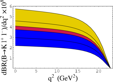
Figure 1: Differential branching fraction $\displaystyle{dBR(B\to K\ell^{+}\ell^{-})/dq^{2}}$ obtained using set A (left) and B (right) of form factors. The dark (blue) region is obtained in SM; the intermediate (red) one for $1/R=500$ GeV, the light (yellow) one for $1/R=200$ GeV. The contribution of $c\bar{c}$ resonances is not displayed.

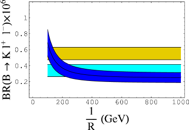
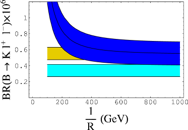
Figure 2: $BR(B\to K\ell^{+}\ell^{-})$ versus $\displaystyle{1\over R}$ using set A (left) and B (right) of form factors. The two horizontal regions correspond to the experimental data provided by BaBar (lower band) and Belle (upper band), see Table 2.

III.2 $B\to K^{*}\ell^{+}\ell^{-}$

A great deal of information can be obtained from the mode $B\to K^{*}\ell^{+}\ell^{-}$ by investigating, together with the lepton invariant mass distribution, also the forward-backward asymmetry ${\cal A}_{fb}$ in the dilepton angular distribution, which may reveal effects beyond the Standard Model that could not be seen in the analysis of the decay rate. In particular, in SM, due to the opposite sign of the Wilson coefficients $C_{7}$ and $C_{9}$, ${\cal A}_{fb}$ has a zero the position of which is almost independent of the model for the form factors Burdman:1998mk .

Let us define $\theta_{\ell}$ as the angle between the $\ell^{+}$ direction and the $B$ direction in the rest frame of the lepton pair (we consider massless leptons). The decay amplitude can be written as sum of non interfering helicity amplitudes, the double differential decay rate reads as follows:

$${d^{2}\Gamma\over dq^{2}dcos\theta_{\ell}} = {G_{F}^{2}|V_{tb}V_{ts}^{*}|^{2}\alpha^{2}\over 2^{13}\pi^{5}}{\lambda^{1/2}(M_{B}^{2},M_{K^{*}}^{2},q^{2})\over M_{B}^{3}}\times\left\{sin^{2}\theta_{\ell}A_{L}+\right.$$ (31)

$$+ \left.q^{2}\left[(1+cos\theta_{\ell})^{2}(A^{L}_{+}+A^{R}_{-})+(1-cos\theta_{\ell})^{2}(A^{L}_{-}+A^{R}_{+})\right]\right\}$$

where $A_{L}$ corresponds to a longitudinally polarized $K^{*}$, while $A^{L(R)}_{+(-)}$ represent the contribution from left (right) leptons and from $K^{*}$ with transverse polarization: $\displaystyle\epsilon_{\pm}=\Big{(}0,{1\over\sqrt{2}},\pm{i\over\sqrt{2}},0\Big{)}$:

$$A_{L}={1\over M_{K^{*}}^{2}}\left\{\left|B_{1}(M_{B}^{2}-M_{K^{*}}^{2}-q^{2})+B_{2}\lambda\right|^{2}+\left|D_{1}(M_{B}^{2}-M_{K^{*}}^{2}-q^{2})+D_{2}\lambda\right|^{2}\right\}$$ (32)

and

$$A^{L}_{\pm}=|\lambda^{1/2}(A-C)\mp(B_{1}-D_{1})|^{2}$$ (33)

$$A^{R}_{\pm}=|\lambda^{1/2}(A+C)\mp(B_{1}+D_{1})|^{2}\;,$$ (34)

where $\lambda=\lambda(M_{B}^{2},M_{K^{*}}^{2},q^{2})$. The terms $A$,$C$,$B_{1}$,$D_{1}$ contain Wilson coefficients and form factors:

$$A={C_{7}\over q^{2}}\,4\,m_{b}\,T_{1}(q^{2})+C_{9}\,{V(q^{2})\over M_{B}+M_{K^{*}}}$$ (35)

$$C=C_{10}\,{V(q^{2})\over M_{B}+M_{K^{*}}}$$ (36)

$$B_{1}={C_{7}\over q^{2}}\,4\,m_{b}\,T_{2}(q^{2})(M_{B}^{2}-M_{K^{*}}^{2})+C_{9}\,A_{1}(q^{2})(M_{B}+M_{K^{*}})$$ (37)

$$B_{2}=-\left[{C_{7}\over q^{2}}\,4\,m_{b}\,\left(T_{2}(q^{2})+q^{2}{T_{3}(q^{2})\over(M_{B}^{2}-M_{K^{*}}^{2})}\right)+C_{9}{A_{2}(q^{2})\over M_{B}+M_{K^{*}}}\right]$$ (38)

$$D_{1}=C_{10}\,A_{1}(q^{2})\,(M_{B}+M_{K^{*}})$$ (39)

$$D_{2}=-C_{10}\,{A_{2}(q^{2})\over M_{B}+M_{K^{*}}}\;.$$ (40)

The forward-backward asymmetry, defined as

$$A^{FB}(q^{2})=\displaystyle{\displaystyle\int_{0}^{1}{d^{2}\Gamma\over dq^{2}dcos\theta_{\ell}}dcos\theta_{\ell}-\int^{0}_{-1}{d^{2}\Gamma\over dq^{2}dcos\theta_{\ell}}dcos\theta_{\ell}\over\displaystyle\int_{0}^{1}{d^{2}\Gamma\over dq^{2}dcos\theta_{\ell}}dcos\theta_{\ell}+\int^{0}_{-1}{d^{2}\Gamma\over dq^{2}dcos\theta_{\ell}}dcos\theta_{\ell}}\;,$$ (41)

reads

$$A^{FB}(q^{2})={3\over 4}{2q^{2}(A^{L}_{+}+A^{R}_{-}-A^{L}_{-}-A^{R}_{+})\over A_{L}+2q^{2}(A^{L}_{-}+A^{R}_{+}+A^{L}_{+}+A^{R}_{-})}\;.$$ (42)

We can now discuss the predictions of the ACD model for the branching ratio as well as for the lepton forward-backward asymmetry. The differential branching ratio is shown in Fig. 3. As in the case of $B\to K\ell^{+}\ell^{-}$. the spectrum is enhanced for lower values of $1/R$, however, due to the hadronic uncertainty, it is not possible to clearly disentangle the extra dimension effect. As for the total rate, depicted in in Fig. 4 for the two sets of form factors, set A does not allow to establish a lower bound on $1/R$, while for set B one gets again $1/R>200$ GeV. The present discrepancy between BaBar and Belle measurements does not permit stronger statements, more precise data from both the experiments are expected.

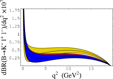
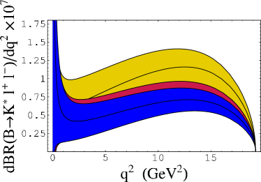
Figure 3: Differential branching fraction $\displaystyle{dBR(B\to K^{*}\ell^{+}\ell^{-})/dq^{2}}$ using set A (left) and B (right) of form factors. The dark (blue) region is obtained in the SM, the intermediate (red) one for $1/R=500$ GeV, the light (yellow) one for $1/R=200$ GeV.

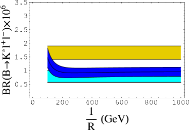
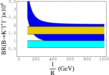
Figure 4: $BR(B\to K^{*}\ell^{+}\ell^{-})$ versus $\displaystyle{1\over R}$ using set A (left) and B (right). The two horizontal regions correspond to BaBar (lower band) and Belle (upper band) results, see Table 2.

More information comes from the forward-backward asymmetry. We show in Fig. 5 the predictions for the SM, $1/R=250$ GeV and $1/R=200$ GeV. The zero of ${\cal A}_{fb}$ is sensitive to the compactification parameter, so that its experimental determination would constrain $1/R$.

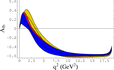
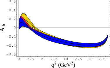
Figure 5: Forward-backward lepton asymmetry in $B\to K^{*}\ell^{+}\ell^{-}$ versus $\displaystyle{1\over R}$ using set A (left) and B (right). The light (yellow) bands correspond to the SM results, the intermediate (red) band to $1/R=250$ GeV, the dark (blue) one to $1/R=200$ GeV.

We can elaborate on this point, since it is easy to see, using (32)-(40) in (42), that the position of the zero of the asymmetry, $s_{0}$, is determined by the equation:

$$Re(C_{9})+{2m_{b}\over s}C_{7}\left[(M_{B}+M_{K^{*}}){T_{1}(s)\over V(s)}+(M_{B}-M_{K^{*}}){T_{2}(s)\over A_{1}(s)}\right]=0\,\,\,.$$ (43)

It is noticeable that, in the large energy limit of the final state light vector meson, a model independent prediction for the position of the zero of the asymmetry can be obtained. As a matter of fact, in this limit the form factors of $B\to P,V$ obey spin symmetry relations Charles:1998dr , broken by hard gluon corrections to the weak vertex and hard spectator interactions. In the heavy-quark limit one can write Beneke:2003pa (see also Hill:2002vw ; Lange:2003pk ; Bauer:2002aj ):

$$\langle P|\bar{\psi}\,\Gamma_{i}\,b|B\rangle=C_{i}(E,\mu_{I})\,\xi_{P}(\mu_{I},E)+T_{i}(E,u,\omega,\mu_{\rm II})\otimes\phi_{+}^{B}(\omega,\mu_{\rm II})\otimes\phi_{P}(u,\mu_{\rm II})+\ldots,$$

where $\Gamma_{i}$ is a generic Dirac structure and the dots stand for sub-leading terms in $\Lambda/m_{b}$. In the case of a vector meson $V$ two functions $\xi_{\perp,\parallel}$ (depending on the Dirac structure $\Gamma_{i}$) appear in place of $\xi_{P}$. The matrix elements in (III.2) get therefore two contributions. The first one contains the short-distance functions $C_{i}$, arising from integrating out hard modes: $\mu_{I}<m_{b}$, and a “soft” form factor $\xi_{P}$ which does not depend on the Dirac structure of the decay current. The second term in (III.2) factorizes into a hard-scattering kernel $T_{i}$ and the light-cone distribution amplitudes $\phi_{B}$ and $\phi_{P}$. A still controversial question is to what extent the first contribution is numerically suppressed by Sudakov effects li , although it has been put forward that the second term in (III.2) should be subleading with respect to the first one Lange:2003pk ; Descotes-Genon:2001hm ; DeFazio:2005dx . Neglecting ${\cal O}(\alpha_{s})$ effects the approximate symmetry relations mentioned above between the vector and tensor form factors for $B\to V$ transitions read Charles:1998dr ; Beneke:2000wa :

$${T_{1}(E)\over V(E)}={1\over 2}{M_{B}\over M_{B}+M_{K^{*}}}\hskip 28.45274pt{T_{2}(E)\over A_{1}(E)}={(M_{B}+M_{K^{*}})\over 2M_{B}}\,.$$ (44)

The use of eq. (44) in (43) produces a form-factor independent result for the position of the zero of the asymmetry: using our numerical input parameters, one would obtain in the Standard Model $s_{0}^{LEET}\simeq 3.61$ GeV². On the other hand, taking into account corrections to the relations in (44), the position of the zero of ${\cal A}_{fb}$ moves to $s_{0}\simeq 4.2\pm 0.6$ GeV² Beneke:2001at .

The dependence of $s_{0}$ on the compactification parameter is depicted in Fig. 6 for the sets A and B of form factors. Two considerations are in order. The first one is that the value of $s_{0}$ in the Standard Model is only marginally consistent with the result obtained in Beneke:2001at , suggesting that further corrections could shift $s_{0}$ to smaller values. The second one concerns the sensible dependence of $s_{0}$ on the compactification parameter: in particular, the zero is pushed to low values by decreasing $1/R$. Such a sensitivity in the exclusive channel is analogous to the one observed in the inclusive $B\to X_{s}\ell^{+}\ell^{-}$ mode, and indicates that $s_{0}$ is particularly suited to constrain $1/R$.

At present, the analysis of the forward-backward lepton asymmetry performed by Belle Collaboration indicates that the relative sign of the Wilson coeffcients $C_{9}$ and $C_{7}$ is negative, confirming that ${\cal A}_{fb}$ should have a zero Abe:2005km . The accurate measurement of $s_{0}$ in the exclusive $B\to K^{*}\ell^{+}\ell^{-}$ channel is therefore within the reach of current experiments.

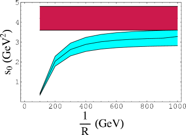
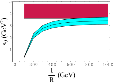
Figure 6: Zero of the forward-backward lepton asymmetry versus $\displaystyle{1\over R}$ obtained using the set A (left) anf B (right) of form factors. In the plots the horizontal region represents the the value of $s_{0}$ derived in Beneke:2001at .

IV The decays $B\to K^{(*)}\nu{\bar{\nu}}$

As mentioned in the Introduction, among the various flavour changing neutral current-induced $b-$quark decays the transitions induced by $b\to s\nu{\bar{\nu}}$ play a peculiar role, both from a theoretical and an experimental point of view. Within the Standard Model these processes are governed by the effective Hamiltonian

$${\cal H}_{eff}={G_{F}\over\sqrt{2}}{\alpha\over 2\pi\sin^{2}(\theta_{W})}\;V_{ts}V^{*}_{tb}\;\eta_{X}X(x_{t})\;{\bar{b}}\gamma^{\mu}(1-\gamma_{5})s\;{\bar{\nu}}\gamma_{\mu}(1-\gamma_{5})\nu\equiv c_{L}^{SM}\;{\cal O}_{L}$$ (45)

obtained from $Z^{0}$ penguin and box diagrams where the dominant contribution corresponds to a top quark intermediate state. In (45) $\theta_{W}$ the Weinberg angle. ${\cal O}_{L}$ represents the left-left four-fermion operator ${\cal O}_{L}\equiv{\bar{b}}\gamma^{\mu}(1-\gamma_{5})s\;{\bar{\nu}}\gamma_{\mu}(1-\gamma_{5})\nu$. The function $X$ has been computed in inami and buchalla ; buchalla1 ; we put to unity the QCD factor $\eta_{X}$ buchalla ; buchalla1 ; Buchalla:1998ba . Possible New Physics (NP) effects can modify the SM value of the coefficient $c_{L}$, or introduce one new right-right operator:

$${\cal H}_{eff}\equiv c_{L}\;{\cal O}_{L}+c_{R}\;{\cal O}_{R}$$ (46)

(${\cal O}_{R}\equiv{\bar{b}}\gamma^{\mu}(1+\gamma_{5})s\;{\bar{\nu}}\gamma_{\mu}(1+\gamma_{5})\nu$), with $c_{R}$ only receiving contribution from phenomena beyond SM Buchalla:2000sk .

Another reason of interest for $b\to s\nu{\bar{\nu}}$ is the absence of long-distance contributions related to four-quark operators in the effective hamiltonian. In this respect, the transition to neutrinos represents a clean process even in comparison with the $b\to s\gamma$ decay, where long-distance contributions are expected to be present, although small Colangelo:1989gi .

Within the Standard Model, form factors are needed to predict branching ratios and decay distributions for the exclusive modes $B\to K^{(*)}\nu{\bar{\nu}}$ (see, e.g. Colangelo:1996ay ; Buchalla:2000sk ). The inclusion of effects stemming from one universal extra dimension is straightforward and requires the generalization of the function $X(x_{t})$ Buras:2002ej :

$$X(x_{t},1/R)=X_{0}(x_{t})+\sum_{n=1}^{\infty}C_{n}(x_{t},x_{n})$$ (47)

where:

$$X_{0}(x_{t})={x_{t}\over 8}\left[{x_{t}+2\over x_{t}-1}+{3x_{t}-6\over(x_{t}-1)^{2}}\ln x_{t}\right]$$ (48)

and $C_{n}(x_{t},x_{n})$ defined in eq. (22).

IV.1 $B\to K\nu{\bar{\nu}}$

It is interesting to consider the missing energy distribution in the decay $B\to K\nu{\bar{\nu}}$. We define $E_{miss}$ the energy of the neutrino pair in the $B$ rest frame and consider the dimensionless variable $x=E_{miss}/M_{B}$, which varies in the range

$${1-r\over 2}\leq x\leq 1-\sqrt{r}$$ (49)

with $r=M_{K}^{2}/M_{B}^{2}$. The differential decay rate is then given by

$${d\Gamma(B\to K\nu\bar{\nu})\over dx}=3\;{|c_{L}+c_{R}|^{2}\,|F_{1}(q^{2})|^{2}\over 48\pi^{3}M_{B}}\sqrt{\lambda^{3}(q^{2},M_{B}^{2},M_{K}^{2})}\;,$$ (50)

where $q^{2}=M_{B}^{2}(2x-1)+M_{K}^{2}$ and the sum over the three neutrino species is understood.

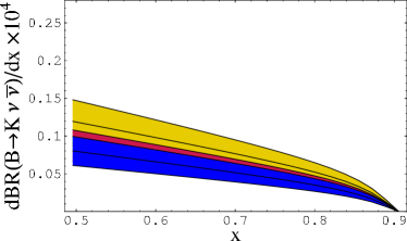
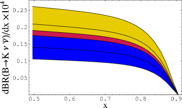
Figure 7: Missing energy distribution in the decay $B\to K\nu{\bar{\nu}}$ for set A (left) and B (right) of form factors. The sum over the three neutrino species is understood. The dark (blue) region is obtained within SM, the intermediate (red) one for $1/R=500$ GeV and the light (yellow) one for $1/R=200$ GeV.

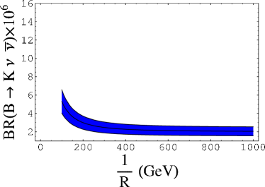
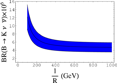
Figure 8: ${BR}(B\to K\nu{\bar{\nu}})$ versus 1/R for set A (left) and B (right) of form factors.

In Fig. 7 we plot the SM missing energy distribution, together with the distributions obtained in ACD for different values of $1/R$. This distribution is sensitive to $1/R$, and the largest effect is in the low-x region, however the hadronic uncertainty is too large for envisaging the possibility of constraining the compactification parameter. As for the branching fraction, its dependence on $1/R$ is shown in Fig. 8. Only an experimental upper bound exist in this channel, which is presently too large for any consideration: however, considering Fig. 8 one sees that the $1/R$ dependence is too mild for distinguishing values above $1/R\geq 200$ GeV.

IV.2 $B\to K^{*}\nu{\bar{\nu}}$

For this mode one can separately consider the missing energy distributions for longitudinally and transversely polarized $K^{*}$:

$${d\Gamma_{L}\over dx}=3\,{|c_{L}|^{2}\over 24\pi^{3}}{|\vec{p}^{~{}\prime}|\over M_{K^{*}}^{2}}\left[(M_{B}+M_{K^{*}})(M_{B}E^{\prime}-M_{K^{*}}^{2})A_{1}(q^{2})-{2M_{B}^{2}\over M_{B}+M_{K^{*}}}|\vec{p}^{~{}\prime}|^{2}A_{2}(q^{2})\right]^{2}\,,$$ (51)

and

$${d\Gamma_{\pm}\over dx}=3{|\vec{p}^{~{}\prime}|q^{2}\over 24\pi^{3}}|c_{L}|^{2}\left|{2M_{B}|\vec{p}^{~{}\prime}|\over M_{B}+M_{K^{*}}}V(q^{2})\mp(M_{B}+M_{K^{*}})A_{1}(q^{2})\right|^{2}\,$$ (52)

where $\vec{p}^{~{}\prime}$ and $E^{\prime}$ are the $K^{*}$ three-momentum and energy in the $B$ meson rest frame and the sum over the three neutrino species is understood. The missing energy distributions for polarized $K^{*}$ are shown in Fig. 9, while the unpolarized distribution and the branching fraction are plotted in Fig. 10 and 11, respectively.

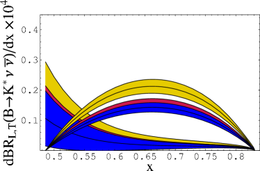
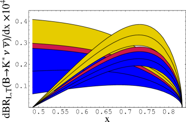
Figure 9: Missing energy distribution in $B\to K^{*}\nu{\bar{\nu}}$ for a longitudinally polarized $K^{*}$ (lower curves) and a transversally polarized $K^{*}$ (upper curves) for set A (left) and B (right) of form factors. The sum over the three neutrino species is understood. The dark (blue) region corresponds to SM, the intermediate (red) one to $1/R=500$ GeV and the light (yellow) one to $1/R=200$ GeV.

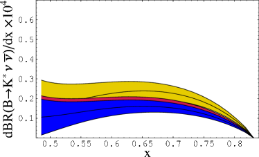
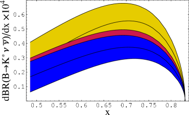
Figure 10: Missing energy distribution for unpolarized $K^{*}$, with the same notations as in Fig. 9.

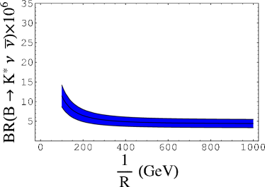
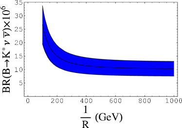
Figure 11: ${BR}(B\to K^{*}\nu{\bar{\nu}})$ versus $1/R$ using set A (left) and B (right) of form factors.

Both the polarized $K^{*}$ and total missing energy distributions depend on $1/R$, but the hadronic uncertainty obscures such an effect as in $B\to K\nu\bar{\nu}$. The dependence of the branching fraction is not strong for $1/R\geq 200$ GeV.

V The decay $B\to K^{*}\gamma$

As a final case we consider the radiative channel $B\to K^{*}\gamma$, which is the first one observed among such rare decay modes. The transition $b\to s\gamma$ is described by the operator $O_{7}$ in the effective hamiltonian (7), and the $B\to K^{*}\gamma$ decay rate is given by:

$$\Gamma(B\to K^{*}\gamma)={\alpha G_{F}^{2}\over 8\pi^{4}}|V_{tb}V_{ts}^{*}|^{2}m_{b}^{2}|C_{7}^{(0)(eff)}|^{2}[T_{1}(0)]^{2}M_{B}^{3}\left(1-{M_{K^{*}}^{2}\over M_{B}^{2}}\right)^{3}\,\,\,.$$ (53)

One can appreciate the consequences of the existence of a single universal extra dimension considering Fig. 12, where the branching fraction is plotted as a function of $1/R$: the sensitivity to the compactification parameter is evident, and it allows to put a lower bound of $1/R\geq 250$ GeV adopting set A, and a stronger bound of $1/R\geq 400$ GeV for set B, which is the most stringent bound that can be currently put on this parameter from the set of $B$ decay modes we have considered.

Figure 12: $BR(B\to K^{*}\gamma)$ versus $\displaystyle{1\over R}$ using set A (left) and B (right) of form factors . The horizontal band corresponds to the experimental result.

VI Conclusions and Perspectives

We have analysed the rare $B\to K^{(*)}\ell^{+}\ell^{-}$, $B\to K^{(*)}\nu\bar{\nu}$, $B\to K^{*}\gamma$ decays in the ACD model with a single universal extra dimension, studying how the predictions for branching fractions, decay distributions and the lepton forward-backward asymmetry in $B\to K^{*}\ell^{+}\ell^{-}$ are modified by the introduction of the fifth dimension. The possibility to constrain the only free parameter of the model, the inverse of the compactification radius $1/R$, are slightly model dependent, in the sense that the constraints are different using different sets of form factors. Nevertheless, various distributions, together with the lepton forward-backward asymmetry in $B\to K^{*}\ell^{+}\ell^{-}$ are very promising in order to constrain $1/R$. We found that the most stringent lower bound comes from $B\to K^{*}\gamma$. Improvements in the experimental data, expected in the near future, will allow to establish more stringent constraints for the compactification radius.

Acnowledgments We thank A.J. Buras for discussions. Two of us (PC and FD) thank CPhT, École Polytechnique, for hospitality during the completion of this work. We acknowledge partial support from the EC Contract No. HPRN-CT-2002-00311 (EURIDICE).

References

(1)
P. Koppenburg et al. [Belle Collaboration],
Phys. Rev. Lett. 93, 061803 (2004).
(2)
B. Aubert et al. [BABAR Collaboration],
Phys. Rev. D 72, 052004 (2005).
(3)
M. Nakao et al. [BELLE Collaboration],
Phys. Rev. D 69, 112001 (2004).
(4)
B. Aubert et al. [BABAR Collaboration],
Phys. Rev. D 70, 112006 (2004).
(5)
M. Iwasaki et al. [Belle Collaboration],
Phys. Rev. D 72, 092005 (2005).
(6)
B. Aubert et al. [BABAR Collaboration],
Phys. Rev. Lett. 93, 081802 (2004).
(7)
K. Abe et al. [Belle Collaboration],
arXiv:hep-ex/0410006.
(8)
B. Aubert et al. [BaBar Collaboration],
arXiv:hep-ex/0507005.
(9)
K. Abe et al. [Belle Collaboration],
arXiv:hep-ex/0507034.
(10)
B. Aubert et al. [BABAR Collaboration],
Phys. Rev. Lett. 94, 101801 (2005).
(11)
A. Ishikawa et al. [The Belle Collaboration],
arXiv:hep-ex/0603018.
(12)
T. Appelquist, H. C. Cheng and B. A. Dobrescu,
Phys. Rev. D 64, 035002 (2001).
(13)
K. Agashe, N. G. Deshpande and G. H. Wu,
Phys. Lett. B 514, 309 (2001).
(14)
A. J. Buras, M. Spranger and A. Weiler,
Nucl. Phys. B 660, 225 (2003).
(15)
A. J. Buras, A. Poschenrieder, M. Spranger and A. Weiler,
Nucl. Phys. B 678, 455 (2004).
(16)
A review of Standard Model predictions can be found in T. Hurth,
Rev. Mod. Phys. 75, 1159 (2003) and in references therein.
(17)
T. Kaluza,
Sitzungsber. Preuss. Akad. Wiss. Berlin (Math. Phys. ) 1921, 966 (1921).
O. Klein,
Z. Phys. 37, 895 (1926)
[Surveys High Energ. Phys. 5, 241 (1986)];
O. Klein,
Nature 118, 516 (1926).
(18)
A. J. Buras, M. Misiak, M. Munz and S. Pokorski,
Nucl. Phys. B 424, 374 (1994).
(19)
C. Bobeth, M. Misiak and J. Urban,
Nucl. Phys. B 574, 291 (2000);
H. H. Asatrian, H. M. Asatrian, C. Greub and M. Walker,
Phys. Lett. B 507, 162 (2001);
Phys. Rev. D 65, 074004 (2002);
Phys. Rev. D 66, 034009 (2002);
H. M. Asatrian, K. Bieri, C. Greub and A. Hovhannisyan,
Phys. Rev. D 66, 094013 (2002);
A. Ghinculov, T. Hurth, G. Isidori and Y. P. Yao,
Nucl. Phys. B 648, 254 (2003);
A. Ghinculov, T. Hurth, G. Isidori and Y. P. Yao,
Nucl. Phys. B 685, 351 (2004);
C. Bobeth, P. Gambino, M. Gorbahn and U. Haisch,
JHEP 0404, 071 (2004).
(20)
M. Misiak,
Nucl. Phys. B 393, 23 (1993)
[Erratum-ibid. B 439, 461 (1995)];
A. J. Buras and M. Munz,
Phys. Rev. D 52, 186 (1995).
(21)
P. Colangelo, F. De Fazio, P. Santorelli and E. Scrimieri,
Phys. Rev. D 53, 3672 (1996)
[Erratum-ibid. D 57, 3186 (1998)].
(22)
P. Ball and R. Zwicky,
Phys. Rev. D 71, 014015 (2005);
Phys. Rev. D 71, 014029 (2005).
(23)
S. Eidelman et al. [Particle Data Group],
Phys. Lett. B 592 (2004) 1.
(24)
[CDF Collaboration],
arXiv:hep-ex/0507091.
(25)
The Heavy Flavour Averaging Group,
http://www.slac.stanford.edu/xorg/hfag/.
(26)
G. Burdman,
Phys. Rev. D 57, 4254 (1998).
(27)
J. Charles, A. Le Yaouanc, L. Oliver, O. Pene and J. C. Raynal,
Phys. Rev. D 60, 014001 (1999).
(28)
M. Beneke and T. Feldmann,
Nucl. Phys. B 685, 249 (2004).
(29)
R. J. Hill and M. Neubert,
Nucl. Phys. B 657, 229 (2003).
(30)
B. O. Lange and M. Neubert,
Nucl. Phys. B 690, 249 (2004)
[Erratum-ibid. B 723, 201 (2005)].
(31)
C. W. Bauer, D. Pirjol and I. W. Stewart,
Phys. Rev. D 67, 071502 (2003).
(32)
R. Akhoury, G. Sterman and Y. P. Yao,
Phys. Rev. D 50, 358 (1994);
M. Dahm, R. Jakob and P. Kroll,
Z. Phys. C 68, 595 (1995);
T. Kurimoto, H. n. Li and A. I. Sanda,
Phys. Rev. D 65, 014007 (2002).
(33)
S. Descotes-Genon and C. T. Sachrajda,
Nucl. Phys. B 625, 239 (2002).
(34)
F. De Fazio, T. Feldmann and T. Hurth,
Nucl. Phys. B 733, 1 (2006).
(35)
M. Beneke and T. Feldmann,
Nucl. Phys. B 592, 3 (2001).
(36)
M. Beneke, T. Feldmann and D. Seidel,
Nucl. Phys. B 612, 25 (2001);
Eur. Phys. J. C 41, 173 (2005).
(37)
T. Inami and C. S. Lim,
Prog. Theor. Phys. 65, 297 (1981)
[Erratum-ibid. 65, 1772 (1981)].
(38)
G. Buchalla and A. J. Buras,
Nucl. Phys. B 400, 225 (1993).
(39)
G. Buchalla, A. J. Buras and M. E. Lautenbacher,
Rev. Mod. Phys. 68, 1125 (1996).
(40)
G. Buchalla and A. J. Buras,
Nucl. Phys. B 548, 309 (1999).
(41)
G. Buchalla, G. Hiller and G. Isidori,
Phys. Rev. D 63, 014015 (2001).
(42)
P. Colangelo, G. Nardulli, N. Paver and Riazuddin,
Z. Phys. C 45, 575 (1990).
(43)
P. Colangelo, F. De Fazio, P. Santorelli and E. Scrimieri,
Phys. Lett. B 395, 339 (1997).